the Creative Commons Attribution 4.0 License.
the Creative Commons Attribution 4.0 License.
 | 03 Dec 2021
CCAM: China Catchment Attributes and Meteorology dataset
Jin Jin
Runliang Xia
Shimin Tian
Wushuang Yang
Qixing Liu
Min Zhu
Tao Ma
Chengran Jing
Yanning Zhang
The absence of a compiled large-scale catchment characteristics dataset is a key obstacle limiting the development of large-sample hydrology research in China. We introduce the first large-scale catchment attribute dataset in China. We compiled diverse data sources, including soil, land cover, climate, topography, and geology, to develop the dataset. The dataset also includes catchment-scale 31-year meteorological time series from 1990 to 2020 for each basin. Potential evapotranspiration time series based on Penman's equation are derived for each basin. The 4911 catchments included in the dataset cover all of China. We introduced several new indicators that describe the catchment geography and the underlying surface differently from previously proposed datasets. The resulting dataset has a total of 125 catchment attributes and includes a separate HydroMLYR (hydrology dataset for machine learning in the Yellow River Basin) dataset containing standardized weekly averaged streamflow for 102 basins in the Yellow River Basin. The standardized streamflow data should be able to support machine learning hydrology research in the Yellow River Basin. The dataset is freely available at https://doi.org/10.5281/zenodo.5729444 (Zhen et al., 2021). In addition, the accompanying code used to generate the dataset is freely available at https://github.com/haozhen315/CCAM-China-Catchment-Attributes-and-Meteorology-dataset (last access: 26 November 2021) and supports the generation of catchment characteristics for any custom basin boundaries. Compiled data for the 4911 basins covering all of China and the open-source code should be able to support the study of any selected basins rather than being limited to only a few basins.
- Article
(12450 KB) - Full-text XML
- BibTeX
- EndNote


Rainfall, interception, evaporation and evapotranspiration, groundwater flow, subsurface flow, and surface runoff are the main components of the terrestrial hydrological cycle. These processes are affected by the nature of the catchment, such as the ability of the soil to hold water. Catchment attributes influence water movement and the storage of the catchment such that hydrologic behaviors can vary across catchments (Van Werkhoven et al., 2008). Studying a large set of terrestrial catchments often provides insights that cannot be obtained when looking at individual cases or small sets (Coron et al., 2012; Kollat et al., 2012; Newman et al., 2015; Lane et al., 2019). For example, a calibrated model may not be applicable in a watershed with vastly different properties. However, by examining a large sample of catchments, it is possible for a data-driven model to learn the similarities and differences among hydrological behaviors across catchments (Kratzert et al., 2019). Prediction in ungauged basins presents a challenging problem in hydrology. The central challenge is how to extrapolate hydrologic information from gauged to ungauged basins, and solving this problem is contingent on understanding the similarities and differences between different catchments. Regionally and temporally imbalanced observations increase the difficulty of the problem. For a model to successfully simulate the ungauged areas, it must adapt itself to the varying hydrologic behaviors present in different catchments. Kratzert et al. (2019) show that encoding catchment characteristics (e.g., soil characteristics, land cover, topography) into a data-driven model can guide the model to behave differently in response to the meteorological time series input based on different sets of catchment attributes.
Large-sample hydrological datasets are the foundation of many hydrological studies (Silberstein, 2006; Shen et al., 2018; Nevo et al., 2019). The term “big hydrologic data” refers to all data influencing the water cycle, such as the meteorological variables, infiltration characteristics of the study area, land use or land cover types, physical and geological features of the study catchment, etc. Many studies are based on large-scale hydrologic data (Coron et al., 2012; Singh et al., 2014b; Berghuijs et al., 2017; Gudmundsson et al., 2019; Tyralis et al., 2019). Basin-oriented datasets are of great significance in hydrological research. For example, comparative hydrology (de Araújo and González Piedra, 2009; Singh et al., 2014a) focuses on understanding how hydrological processes interact with the ecosystem – in particular, how hydrologic behaviors change in response to changes in the surface and subsurface of the earth to determine to what extent hydrological predictions can be transferred from one area to another. Large-sample catchment attribute datasets provide opportunities to research interrelationships among catchment attributes. Seybold et al. (2017) study the correlations between river junction angles and geometric factors, downstream concavity, and aridity. Oudin et al. (2008) investigate the link between land cover and mean annual streamflow based on 1508 basins representing a large hydroclimatic variety. Voepel et al. (2011) examine how the interaction of climate and topography influences vegetation response.
Worldwide data sharing has become a trend (Lehner et al., 2008; Ceola et al., 2015; Blume et al., 2018; Wang et al., 2020), and the amounts of hydrologic data available are ever increasing. However, these data typically come from different providers and are compiled in various formats. ASTGTM (Abrams et al., 2020) provides a global digital elevation model; GLiM (Global Lithological Map; Hartmann and Moosdorf, 2012) includes rock type data globally; MODIS (Moderate Resolution Imaging Spectroradiometer) provides data products (Didan, 2015; Knyazikhin, 1999; Myneni et al., 2015; Running and Mu, 2017; Sulla-Menashe and Friedl, 2018) that describe features of the land and the atmosphere derived from remote sensing observations; Yamazaki et al. (2019) provide a global flow direction map at 3 arcsec resolution; HydroBASINS (Lehner, 2014) provides basin boundaries at different scales globally; GDBD (Global Drainage Basin Dataset; Masutomi et al., 2009) provides basin boundaries with geographic attributes; GLHYMPS (GLobal HYdrogeology MaPS; Gleeson et al., 2014) provides a global map of subsurface permeability and porosity; and the SoilGrids (Hengl et al., 2017) dataset provides global numeric soil properties. Local government agencies often hold meteorological data such as precipitation and evaporation, and the amount of these data is also growing.
However, the data mentioned above are rarely spatially aggregated to the catchment scale, making it difficult for researchers to use them. Properly preprocessed and formatted datasets are of great importance in hydrology research. Searching for appropriate data sources, preprocessing, and formatting often consume considerable time. In some cases, individual research groups either do not know where to obtain the appropriate data or cannot properly process the data into the desired format. In summary, although data sharing is being advocated in the community, it is usually difficult for the public to obtain the required data, either because there are insufficient observations or because of the difficulties associated with data processing.
Recently, there have been efforts (Addor et al., 2017; Alvarez-Garreton et al., 2018; Chagas et al., 2020; Coxon et al., 2020) to compile different types of data sources to form large-scale hydrological datasets. These four collected datasets cover the continental United States, Chile, Brazil, and Great Britain. Addor et al. (2020) review these datasets and discuss the guidelines for producing large-sample hydrological datasets and the limitations of the currently proposed datasets. The static properties of 671 river basins in the United States are calculated by CAMELS (Addor et al., 2017), which is an extension of a previously proposed hydrometeorological dataset (Newman et al., 2015). Unfortunately, it is impossible to publish streamflow data in China at present. The CAMELS dataset has been used to support much research. For example, Knoben et al. (2019) compare metrics used in hydrology based on simulations in many basins. Tyralis et al. (2019) study the relationship between shape parameters and basin attributes based on a sizeable basin-oriented dataset.
There is currently no compilation of China-specific catchment attribute datasets. An alternative – the HydroATLAS (Linke et al., 2019) dataset, which is on a global scale – basically performs zonal statistics on the source data. HydroATLAS lacks many indicators that make derivations from source data, such as rainfall seasonality, the proportion of precipitation falling as snow, basin shape factors, and root depth distributions. Moreover, the meteorological data are only up to the year 2000, which is outdated.
In summary, a lack of a compiled catchment attribute dataset is a key obstacle limiting the development of large-sample hydrology research in China. Inspired by Addor et al. (2017), we compiled multiple data sources, including basin topography, climate indices, land cover characteristics, soil characteristics, and geological characteristics. Unlike Addor et al. (2017), the catchments included in the dataset cover the entire study area instead of being limited to a few data sources.
The proposed dataset is the first dataset that provides catchment meteorological time series and catchment attributes of China. We compiled and named the dataset following most standards set by the previously proposed datasets. The dataset consists of all derived basin boundaries from the digital elevation model (DEM), which is a subset of the Global Drainage Basin Dataset (GDBD; Masutomi et al., 2009). The GDBD is derived at high resolution (100 m–1 km) and has good geographic agreement with existing global drainage basin data in China. In addition, previously proposed datasets (Addor et al., 2017; Alvarez-Garreton et al., 2018; Chagas et al., 2020; Coxon et al., 2020) report only the most frequent catchment land cover and lithology types. By contrast, CCAM (China Catchment Attributes and Meteorology) calculates the proportions of all land cover and lithology types.
In addition to the basinwise attributes provided in CCAM, we propose HydroMLYR (hydrology dataset for machine learning in the Yellow River Basin), a hydrology dataset for machine learning research in the Yellow River Basin (YRB) providing weekly averaged standardized streamflow data for 102 basins in the YRB. HydroMLYR is proposed to support machine learning hydrology research in the YRB. Traditional hydrological models face long-standing challenges, such as their inability to capture hydrological process mechanism complexity (Kollat et al., 2012), which is due to the structural limitations of the conceptual models. Data-driven strategies represented by machine learning are proposed to overcome some existing obstacles, and these strategies offer a new way for researchers to acquire knowledge capable of transforming the research pattern from hypothesis-driven to data-driven. Feng et al. (2020) propose a flexible data integration fusing various types of observations to improve rainfall-runoff modeling. Their research shows that combining different data resources improves predictions in regions with high autocorrelation in streamflow. Wongso et al. (2020) develop a model predicting the state-level per capita water use in the United States, taking various geographic, climatic, and socioeconomic variables as input. Their research also identifies key factors associated with high water usage. Mei et al. (2020) propose a statistical framework for spatial downscaling to obtain hyperresolution precipitation data. Their results show improvements compared with the original product. Brodeur et al. (2020) apply machine learning techniques – namely, bootstrap aggregation and cross-validation – to reduce overfitting in reservoir control policy search. Ni and Benson (2020) propose an unsupervised machine learning method to differentiate flow regimes and identify capillary heterogeneity trapping and show the promise of machine learning methods for analyzing large datasets from core flooding experiments. Legasa and Gutiérrez (2020) propose applying a Bayesian network for multi-site precipitation occurrence generation, and the proposed methodology shows improvements over existing methods. The proposed dataset can be used to develop or verify machine learning models in the YRB.
This paper is organized as follows. Section 2 describes the study area. Sections 3–7 describe the five classes of computed catchment attributes. Section 8 describes the proposed catchment-scale meteorological time series. Section 9 introduces the HydroMLYR dataset. Section 10 describes the code and data availability. Section 11 is our concluding remarks.
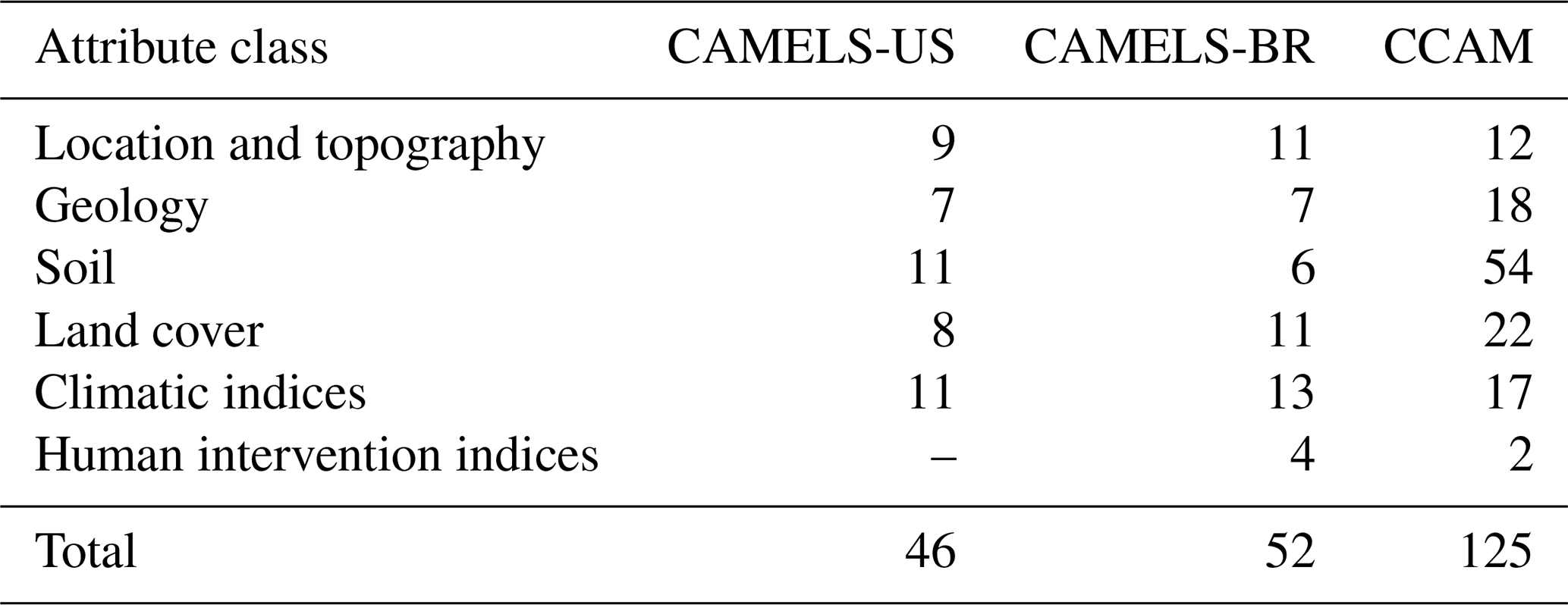
The study area corresponds to the whole of China (Fig. 1), which is characterized by diverse climate and terrain characteristics and spans from 18.2 to 52.3∘ N and 76.0 to 134.3∘ E. Mountains, plateaus, and hills account for approximately two-thirds of the area of China, and the remaining areas are basins and plains. China's topography is similar to a three-level ladder in that it is high in the west and low in the east. The Qinghai–Tibet Plateau, which is located in western China and is the highest plateau globally with a mean elevation of over 4000 m, is the first step of China's topography. The Xinjiang region, the Loess Plateau, the Sichuan Basin, and the Yunnan–Guizhou Plateau to the north and east are the second steps of China's topography. The mean sea level here is between 1000 and 2000 m. Plains and hills dominate the third step. Gorge Mountains, Dahingganling, Tai-hang Mountains, and Xuefengshan compose the boundary between the second and third step. The elevation of this step descends to 500–1000 m. To better characterize the studied catchments, we derived various attributes. Table 1 compares the number of derived attributes between several proposed datasets.
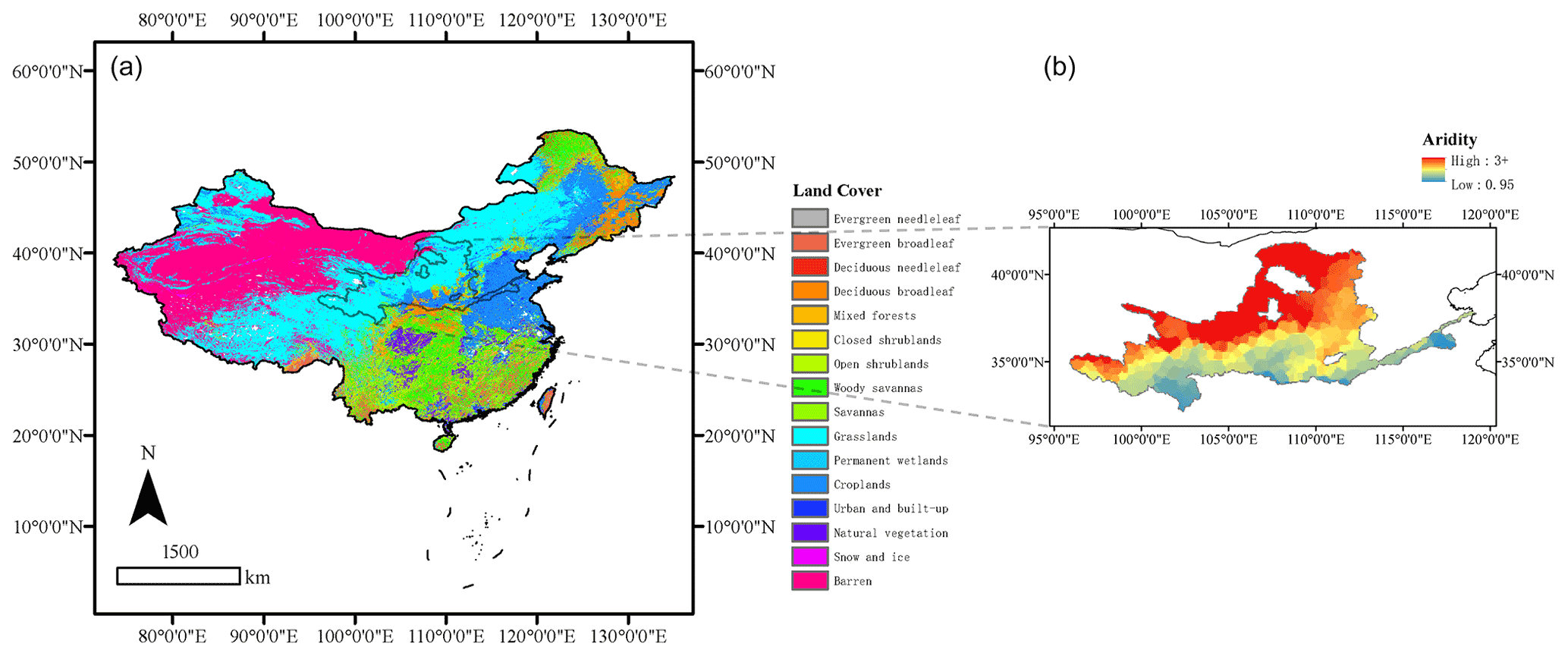
Figure 1(a) Study area of CCAM and the distribution of land cover types. The studied basins cover the whole of China. (b) Study area of HydroMLYR and the distribution of aridity (PET/P) index. YRB is a generally arid area. The dataset provided can be used as a good sample for studying hydrology in arid regions.
Table 1Number of computed attributes in CAMELS, CAMELS-BR, and CCAM.
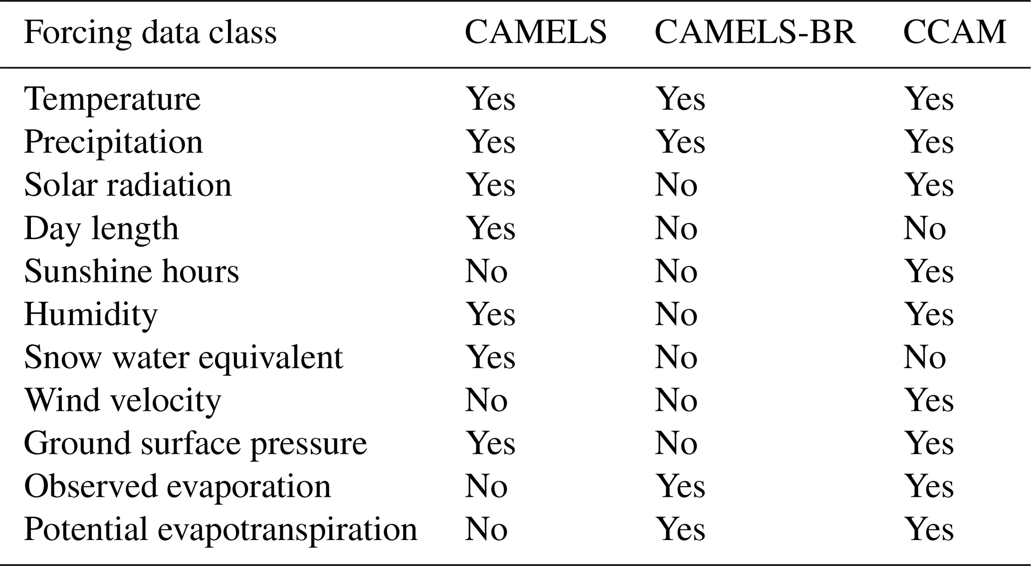
In China, precipitation and temperature vary significantly throughout the country, which forms a diverse climatic environment. According to the Köppen climate classification system, moving from northwest to southeast, China's climate gradually evolves from a cold desert (BWk) climate, a tundra (ET) climate, and a warm and temperate continental (Dfa and Dwb) climate to a humid subtropical (Cwa) climate and warm oceanic (Cfa) climate. There are humid, semi-humid, semiarid, and arid regions from the perspective of wet vs. dry zones. Moreover, the same temperature zone can contain multiple dry and wet zones. Therefore, there may be differences in heat and wetness in the same climate type. The complexity of the terrain makes the climate even more complex and diverse. In addition, China has a wide range of regions which are affected by alternating winter and summer monsoons. Compared with other parts of the world at the same latitude, these areas have lower winter temperatures, higher summer temperatures, significant annual temperature differences, and concentrated precipitation in summer. The cold and dry winter monsoon occurs in Asia's interior, far from the ocean. Winter rainfall in most parts of China is low and accompanied by low temperatures. The summer monsoon is warm and humid and comes from the Pacific and Indian oceans. Precipitation generally increases during this time. Table 2 compares the provided forcing variables in CAMELS (US), CAMELS-BR (Brazil), and CCAM.
Table 2Summary of forcing variables provided in CAMELS, CAMELS-BR, and CCAM.
Raw meteorological data are provided by the China Meteorological Data Network and released as the SURF_CLI_CHN_MUL_DAY (V3.0) dataset, which provides the longest period (1951–2020) of meteorological time series in China. The SURF_CLI_CHN_MUL_DAY product includes site observations of pressure, temperature, relative humidity, precipitation, evaporation, wind speed, sunshine duration, and ground surface temperature (Table 3). The inverse distance weighting method is used to interpolate the site observations. To ensure data quality, we use the latter 31-year record (from 1990 to 2020) to construct the dataset since the site distribution was sparse in the early observations (Fig. 2). We computed more climatic characteristics than most other datasets (Table 2). These variables are useful in hydrological modeling; for example, wind speed can affect actual evapotranspiration. To remain consistent with CAMELS (Addor et al., 2017), we determined all climatic attributes (Woods, 2009) provided in the CAMELS dataset. As a result, the proposed dataset provides more meteorological variables and a longer time series (1990–2020) than CAMELS and CAMELS-CL. A summary of the derived climate indices is presented in Table A1. Figure 3 illustrates the national distributions of the climate indicators.
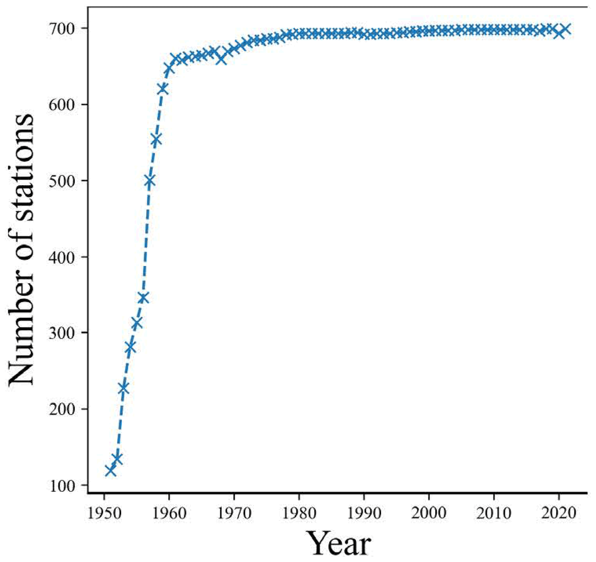
Figure 2Changes in the number of meteorological stations in China. There were only 119 stations in 1951. This number increased rapidly from 1951 to the early 1960s, and the number of stations remained stable after 2000. To ensure data quality, we used the latter 31 years (from 1990 to 2020) to construct the dataset.
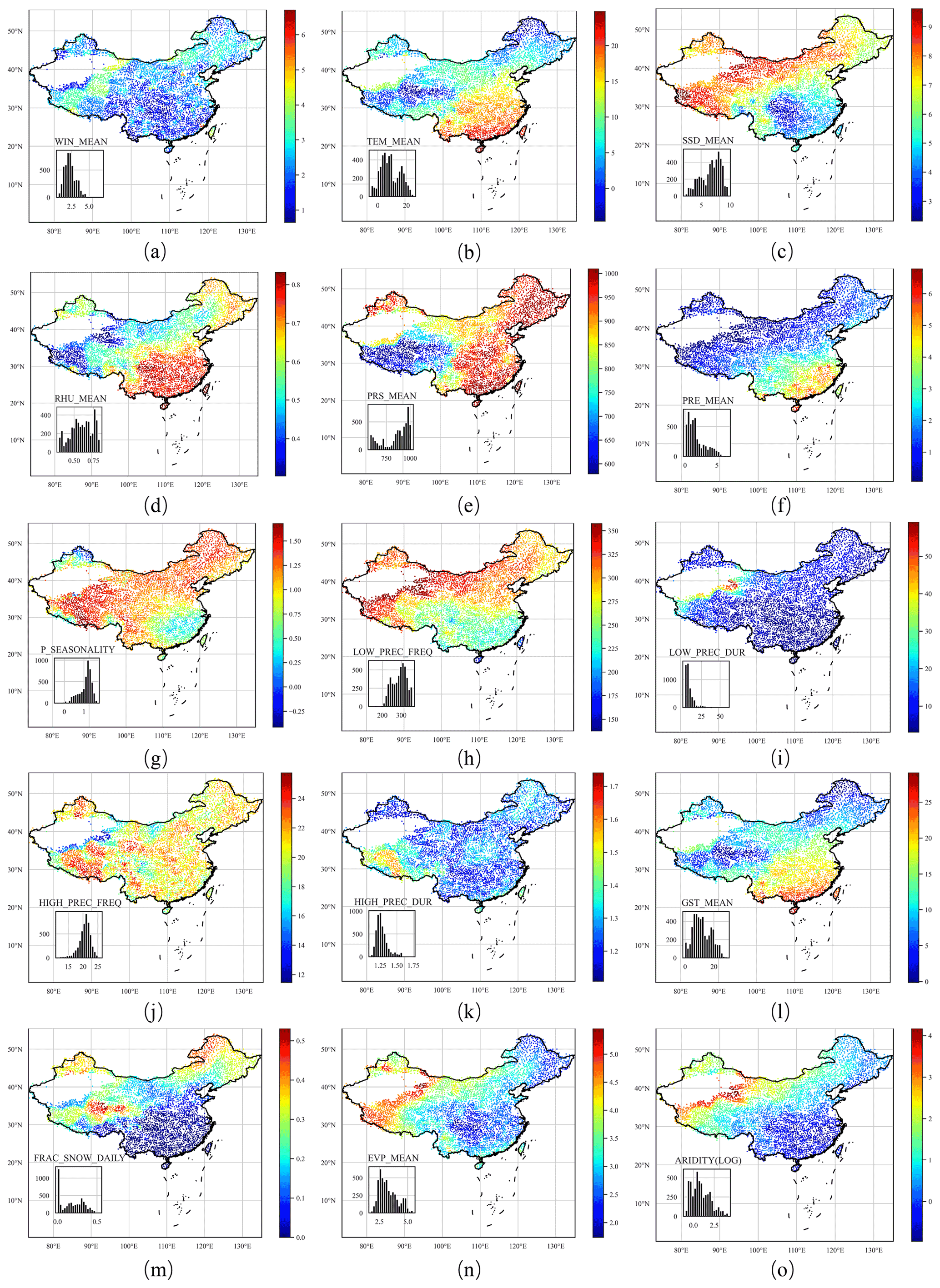
Figure 3Distributions of climatic indices throughout China. All basins are plotted in the same size. When extreme values of a variable affect visualization (causing most areas to have the same color), the log values are used for visualization.
The instruments used to measure potential evaporation were updated from 2000 to 2005. Early observations can be multiplied by a correction coefficient to approximate the new tools. However, the coefficient varies across stations, making the approach infeasible. To complement this, we calculated potential evapotranspiration (PET) based on a modified Penman's equation (Appendix B) and other observed meteorological variables, which provides a series of consistent potential evaporation estimations for reference.
The average daily precipitation in China is highest in the southeast and lowest in the northwest. It is also higher in coastal areas than in the interior. Ground surface pressure is positively correlated with elevation and is highest on the Qinghai–Tibet Plateau and the lowest in the southeast plain. The average relative humidity is generally positively correlated with precipitation; it is also higher in some forested areas, such as the Tai-hang mountains and the Dahingganling. The Qinghai–Tibet Plateau has the lowest average temperature, and the southern coastal area has the highest. A distinctive feature of the distribution of wind speed is the high wind speed in mountainous areas. The highest wind speed occurs in the southeast coastal area (> 6 m s−1).
To describe the lithological characteristics of each catchment, we used the same two global datasets as CAMELS: Global Lithological Map (GLiM) (Hartmann and Moosdorf, 2012) and GLobal HYdrogeology MaPS (GLHYMPS) (Gleeson et al., 2014). Figure 4 illustrates the distributions of the geological types.
GLiM provides a high-resolution global lithological map assembled from existing regional geological maps; it has been widely used to construct datasets (e.g., SoilGrids; Hengl et al., 2017). However, the data quality of GLiM can vary among spatial locations depending on the quality of the original regional geological maps. GLiM consists of three levels: the first level contains 16 lithological classes, and the additional two levels describe more specific lithological characteristics. The GLiM is represented by 1 235 400 polygons which are converted to raster format for the basin-scale lithological type statistics. For China, the compiled regional data sources (MGC, 1991; BGX, 1992; CGS, 2001) have slightly lower resolutions than the GLiM target resolution (1:1 000 000). However, for a basin-scale study with a mean basin area of over 2000 km2, the classification accuracy should satisfy most applications. In contrast to CAMELS and CAMELS-CL, we determined each lithological class's contribution to the catchment instead of recoding the first and second most frequent classes only.
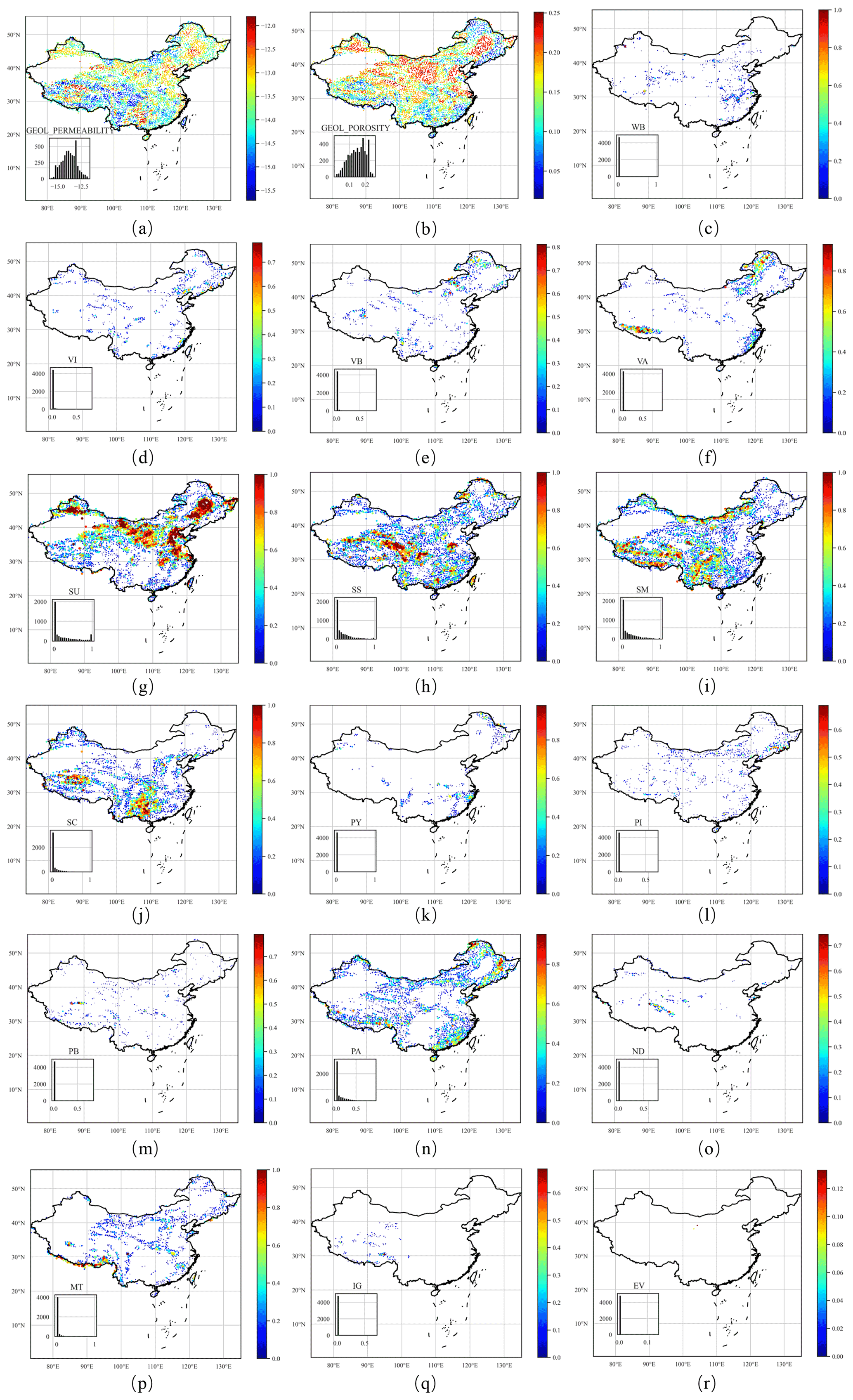
Figure 4Distributions of geological characteristics throughout China. For lithologies, the plot size is scaled by the lithology proportion.
GLHYMPS provides a global estimation of subsurface permeability and porosity, two critical characteristics for soil hydrological classification. Porosity and permeability influence an area's infiltration capacity. Soil with high porosity is likely to contain more water, and highly permeable soil transmits water relatively quickly. Based on the high-resolution map of GLiM, which can differentiate fine- and coarse-grained sediments and sedimentary rocks, GLHYMPS determines subsurface permeability depending on the different permeabilities of rock types. For the proposed dataset, we calculated the catchment arithmetic mean for porosity. Following Gleeson et al. (2011), the logarithmic scale geometric mean is used to represent the subsurface permeability. A summary of the geological characteristics is presented in Table A1.
Porosity and permeability have distributions similar to those of the geological classes. These two characteristics are highly dependent on rock properties; unconsolidated sediments, mixed sedimentary rocks, siliciclastic sedimentary rocks, carbonate sedimentary rocks, and acid plutonic rocks are the five most common geological classes in China. Unconsolidated sediment is the most common rock type in China as it is dominant in 31.9 % of catchments and extends from Xinjiang inland to the northeast and the coastal area surrounding the Bohai Sea. Due to the high proportion of unconsolidated sediments present in the rock, these areas typically have high permeability and medium porosity. Mixed sedimentary rocks are the second most common rock type in China, accounting for 20.3 % of catchments, and they are predominantly on the southern Qinghai–Tibet Plateau, on the western Yunnan–Guizhou Plateau, and in northern Inner Mongolia. These areas typically have high porosity and low permeability. Siliciclastic sedimentary rocks are found in 17.7 % of basins and are mainly distributed in the northern part of the Qinghai–Tibet Plateau and the junction of the Qinghai–Tibet and the Yunnan–Guizhou plateaus; there are also observations in the eastern inland region. These areas have low subsurface permeability and high subsurface porosity. Among all catchments, 9.8 % are dominated by carbonate sedimentary rocks, which are mainly located in eastern Yunnan and on the northern Qinghai–Tibet Plateau. Acid plutonic rocks are typically distributed in the mountains surrounding the inland northeast – namely, the Dahingganling and the hills in southern Guangdong and southwestern Guangxi. They are also distributed along the Brahmaputra River in the southern part of the Qinghai–Tibet Plateau. The distribution of acid plutonic rocks is relatively scattered; there are many isolated acid plutonic rock distributions throughout China which are characterized by medium permeability and high porosity.
The types of rocks in China are dominated by unconsolidated sediments and mixed sedimentary rocks. In 33.86 % of the catchments, the dominant rock types occupy less than 50 % of the catchment areas, and only 16.8 % of basins have a dominant rock type with an area proportion greater than 90 %. Among 4911 basins, 9.4 % have prevalent rock types that occupy the area.
We selected two indicators to characterize surface vegetation density and growth: the normalized difference vegetation index (NDVI) and the leaf area index (LAI). NDVI is an indicator with a valid range of −0.2 to 1 that assesses whether the area being observed contains live green vegetation and the plants' overall health. However, NDVI is only a qualitative measurement of vegetation density and cannot provide a quantitative estimate of the vegetation density in the area. Moreover, NDVI often provides inaccurate vegetation density measurements, and only long-term measurements and comparisons can ensure its accuracy. NDVI alone is not enough to estimate the state of the vegetation in an area. Therefore, we selected another indicator, LAI, to supplement the deficiencies of NDVI.
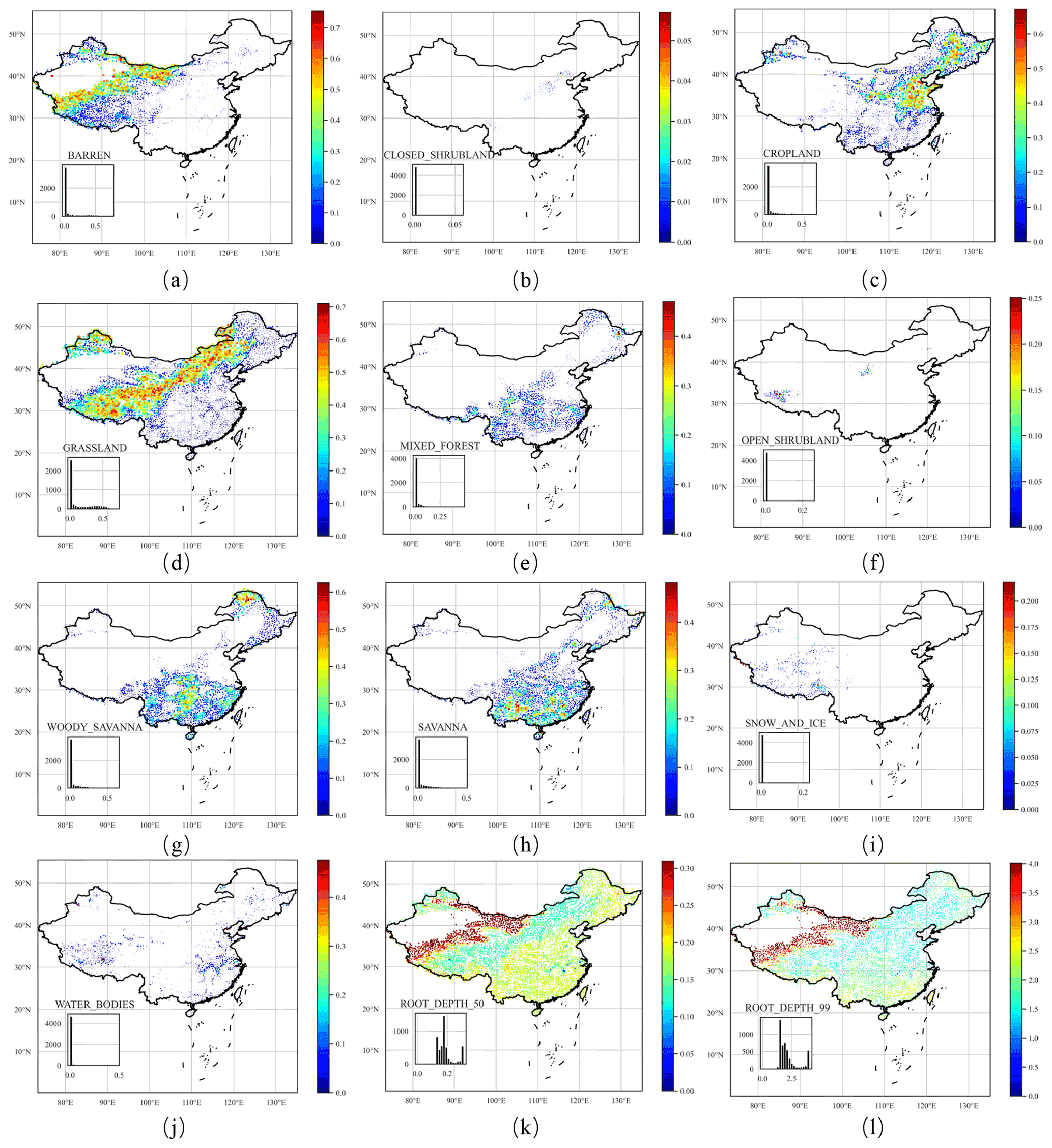
Figure 5Distributions of land cover characteristics throughout China. For land cover types, the plot size is scaled by the size of the land cover proportion.
LAI is defined as the total needle surface area per unit of ground area and half of the entire needle surface area per unit of ground surface area. It is a quantifiable value that is functionally related to many hydrological processes, such as water interception (Van Wijk and Williams, 2005). Buermann et al. (2001) verify the validity of the LAI for characterizing vegetation growth. The data sources used are the Terra Moderate Resolution Imaging Spectroradiometer Vegetation Indices (Didan, 2015) for NDVI and the Moderate Resolution Imaging Spectroradiometer (MODIS) (Myneni et al., 2015) for LAI. Following Addor et al. (2017), we determined the maximum monthly LAI as an indicator that characterizes the vegetation interception capacity, the maximum evaporative capacity, and the difference between the maximum and minimum monthly LAI, which represents the LAI's temporal variations.
Land cover classification refers to segmenting the ground into different categories based on remote sensing images. The Terra and Aqua combined MODIS land cover type provides different results depending on the classification system used. The Annual International Geosphere–Biosphere Programme (IGBP) classification is used to build the dataset, which is derived by the c4.5 decision tree algorithm. The IGBP classification system was formulated by the IGBP Land Cover Working Group in 1995, resulting in 17 categories of land cover types (Belward et al., 1999). Friedl et al. (2010) compare the IGBP data of MODIS with other reference datasets and conclude that the MODIS classification of IGBP has an accuracy of 75 %. We determined the fraction of each land cover class for each basin based on the Terra and Aqua combined Moderate Resolution Imaging Spectroradiometer (MODIS) land cover type (Sulla-Menashe and Friedl, 2018), which differentiates our dataset from CAMELS and CAMELS-CL (which only calculate the proportion of the dominant types).
Following Addor et al. (2017), we computed the average rooting depth (50 % and 90 %) for each catchment based on the IGBP classification using a two-parameter method (Zeng, 2001). The root depth distribution of vegetation affects the ground water holding capacity and the topsoil layer's annual evapotranspiration (Desborough, 1997). Many models use root depth as an essential parameter to characterize soil moisture absorption capacity. Zeng (2001) developed a two-parameter asymptotic equation to estimate root depth distribution, which is global and derived from the IGBP classification to avoid the problem of significantly different root distributions in various research efforts. Figure 5g shows root depth distributions of different vegetation types based on Zeng (2001). The 90 % root depth is usually considered to be “rooting depth”; among the 17 categories of IGBP, cropland has the smallest rooting depth, and open shrubland has the largest. The 90 % root depth of all vegetation is less than 2 m. The national distribution of catchment soil characteristics is shown in Fig. 5.
The catchment boundary files are obtained from the global drainage basin dataset (Masutomi et al., 2009). The GDBD dataset was derived from digital elevation models (DEMs) with a high resolution (100 m–1 km), and the errors were corrected by either automatic methods or manually. Additionally, GDBD also provides population and population density estimates for catchments, and these two indicators are also included in our dataset as a measure of human intervention. Global Runoff Data Centre (GRDC; https://www.bafg.de/GRDC/EN/01_GRDC/grdc_node.html, last access: 26 November 2021) discharge gauging stations were used to reference the derived basins. GDBD has a high average match area rate (AMAR) and good geographic agreement with existing global drainage basin data in China. Precise geographic and topographic information can be derived from the high-quality dataset.
The topography attributes of each catchment are determined by the ASTGTM product retrieved from https://lpdaac.usgs.gov (last access: 26 November 2021) and maintained by the NASA EOSDIS Land Processes Distributed Active Archive Center (LP DAAC) at the USGS Earth Resources Observation and Science (EROS) Center.
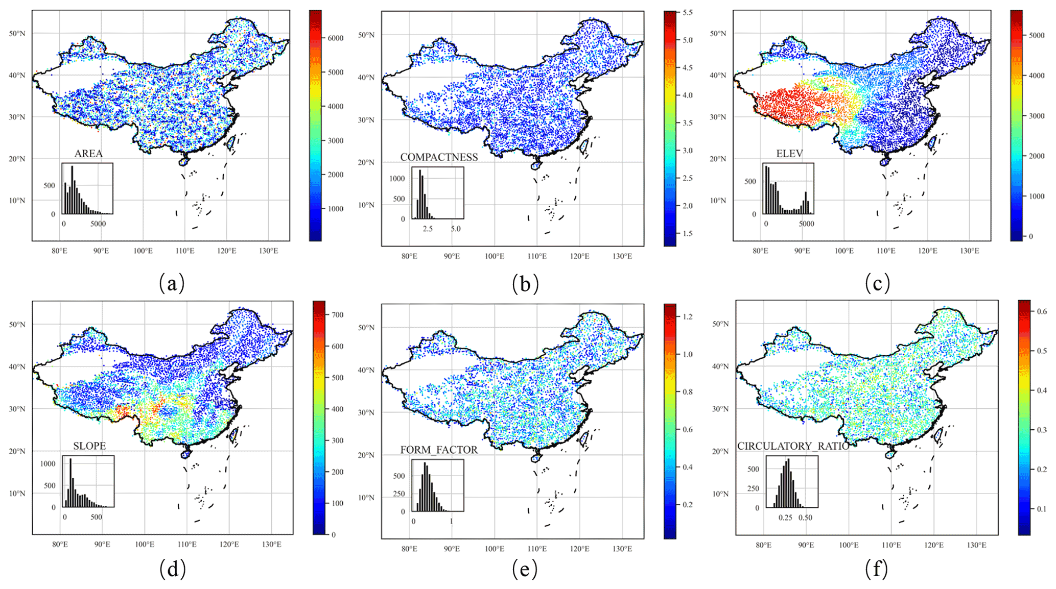
Figure 6Distributions of topographic characteristics throughout China.
The CAMELS dataset provides two parameters (i.e., two area estimates) to describe the catchment shape. The physical characteristics of a catchment can affect the streamflow volume and the streamflow hydrograph of the catchment in a storm. To provide a complete description of the catchment shape, we computed several geometrical parameters of the catchment related to the runoff (Fig. 6), including the catchment form factor, shape factor, compactness coefficient, circulatory ratio, and elongation ratio (Subramanya, 2013). A summary can be found in Table A1.
The proposed dataset has a total of 54 soil attributes (Table A1) derived from Hengl et al. (2017), Dai et al. (2019), and Shangguan et al. (2013). Five categories of soil characteristics (pH in H2O, organic carbon content, depth to bedrock, cation exchange capacity (CEC), and bulk density) are determined from SoilGrids. SoilGrids (Hengl et al., 2017) provides global predictions for soil properties, including organic carbon, bulk density, CEC, pH, soil texture fractions, and coarse fragments, by fusing multiple data sources, including MODIS land products, Shuttle Radar Topography Mission (SRTM) DEM, climatic images, and global landform and lithology maps, at 250 m resolution (Fig. 7). SoilGrids makes predictions using machine learning algorithms and many covariate layers primarily derived from remote sensing data and has soil characteristics at several soil depths.
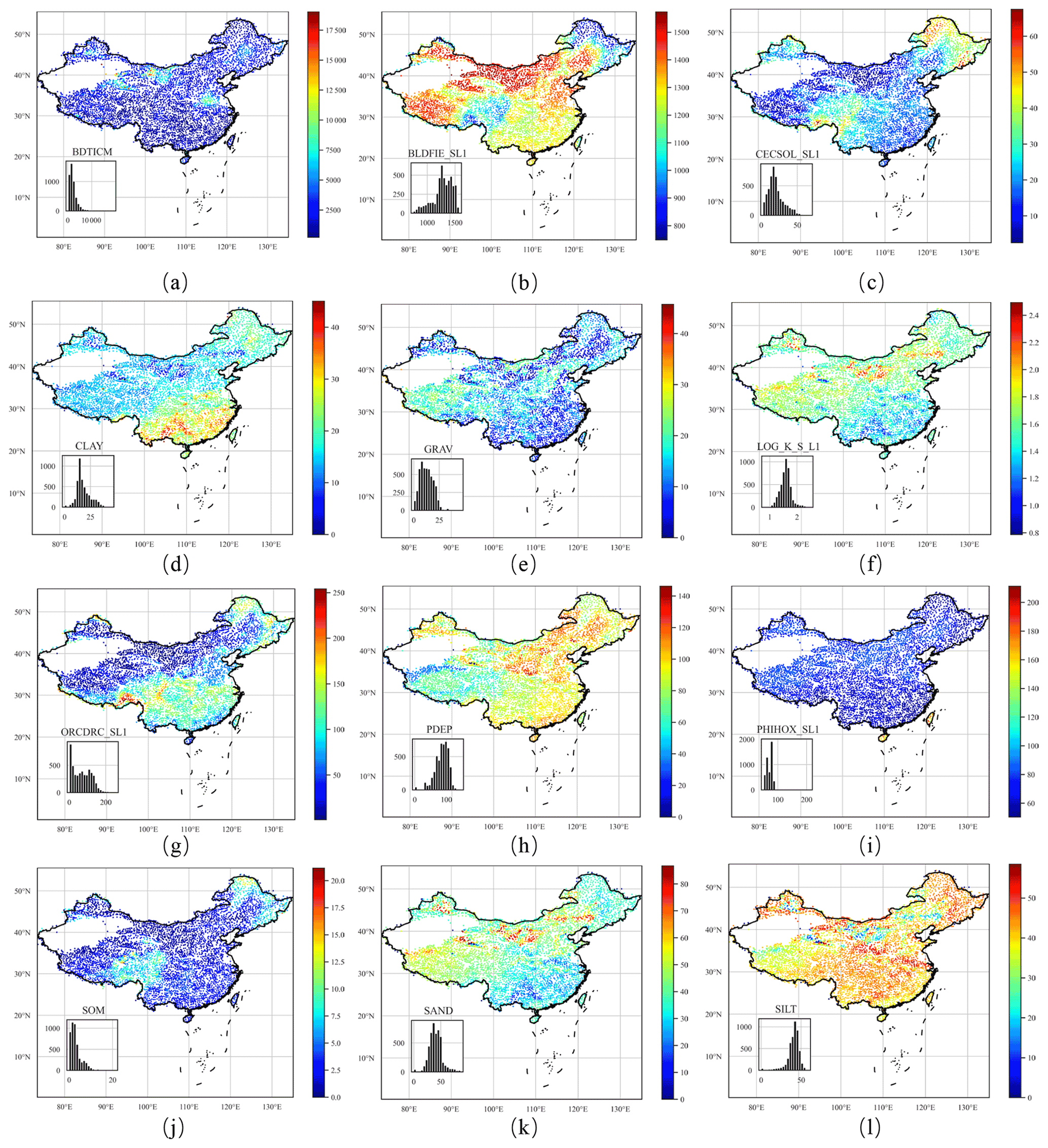
Figure 7Distributions of soil characteristics throughout China.
Unlike CAMELS, whose reported results are obtained by a linear weighted combination of the different soil layers, and CAMELS-BR, whose products are soil characteristics at a depth of 30 cm, we computed soil characteristics at all soil layers provided by SoilGrids.
We determined the saturated water content and saturated hydraulic conductivity (Dai et al., 2019). Based on the same dataset, we also introduced the thermal conductivity of unfrozen saturated soils. Dai et al. (2019) provide a global estimation of soil hydraulic and thermal parameters using multiple pedotransfer functions (PTFs) based on the SoilGrids dataset. Based on the SoilGrids and GSDE (Global Soil Dataset for Earth System Models; Shangguan et al., 2014) datasets, Dai et al. (2019) produce six soil layers with a spatial resolution of 30×30 arcsec. Their vertical resolution is the same as that of SoilGrids, with six intervals of 0–0.05, 0.05–0.15, 0.15–0.30, 0.30–0.60, 0.60–1.00, and 1.00–2.00 m. We determined and recorded catchment soil characteristics for all these layers. In addition, we determined seven more soil characteristics (Shangguan et al., 2013), including soil profile depth, porosity, clay/silt/sand content, rock fragment, and soil organic carbon content. Shangguan et al. (2013) provide the physical and chemical attributes of soils derived from 8979 soil profiles at a 30×30 arcsec resolution using the polygon linkage method to derive the spatial distribution of soil properties. The profile attribute database and soil map are linked under a framework to avoid uncertainty in taxon referencing.
Depth to bedrock controls many physical and chemical processes in soil. The distribution of depth to bedrock in China is characterized by (i) low values in mountainous areas, such as Yunnan Province and the city of Chongqing, and (ii) high values in barren areas, such as north and northwest China. The introduced soil pH value is crucial since it influences many other physical and chemical soil characteristics. The spatial variability in soil pH in China is characterized by (i) soils in southern China being acidic to strongly acidic, (ii) soils in northern China being natural or alkaline, and (iii) soils in northeastern forested areas also being acidic (pH < 7.2). Cation exchange capacity can be seen as a measure of soil fertility since it measures how much nutrient content the soil can store such that it influences the growth of vegetation. Cation exchange capacity is positively correlated with soil organic matter (SOM) and clay content and is generally low in sandy and silty soils. The spatial variability in cation exchange capacity in China is characterized by (i) high values in peat and forested areas on the Qinghai–Tibet Plateau and in central and northeast China and (ii) extremely low cation exchange capacity in desert areas such as the northwest. Soil hydraulic and thermal properties are greatly affected by SOM. Soil organic matter has a similar distribution to cation exchange capacity in that it is high in the peat and forested areas in northeast China and low in the north and northwest.
Table 3Summary table of catchment meteorological time series available in the proposed dataset.
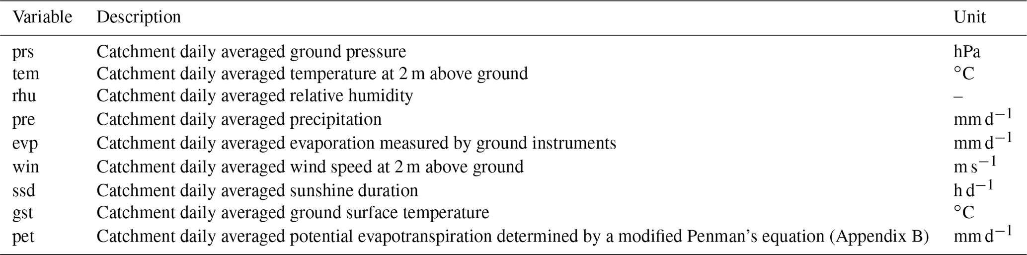
There have been many studies based on SURF_CLI_CHN_MUL_DAY in China (Xu et al., 2009; Liu et al., 2004; Huang et al., 2016; Liu et al., 2017), such as a trend analysis of pan evaporation (Liu et al., 2010). Nevertheless, there has not yet been a large-scale basin-oriented meteorological time series dataset in China. Researchers need to complete multiple iterations to extract historical meteorological data from the SURF_CLI_CHN_MUL_DAY dataset for this type of research. For the first time, we release a catchment-scale meteorological time series dataset. The open-source code can generate any catchment's meteorological time series within China. The basin-oriented dataset provides meteorological time series for 4911 basins from 1990 to 2020 based on the China Meteorological Data Network source. Meteorological time series include pressure, temperature, relative humidity, precipitation, evaporation, wind speed, sunshine duration, ground surface temperature, and potential evapotranspiration (Table 3).
The meteorological time series data from 1951 to 2010 are derived based on the “1951–2010 China National Ground Station Data Corrected Monthly Data File Basic Data Collection” data construction project. Other data include monthly reported data to the National Meteorological Information Centre by province and hourly and daily data uploaded by automatic ground stations in real time. During the construction of the dataset, missing data were filled by interpolating to the nearest stations.
Figure 2 illustrates the variation in the number of sites. The earliest recording was in 1951, but because the early site distribution was sparse, we only used records from 1990 to 2020 to ensure data quality. Inverse distance weighting shows better performance than other interpolation methods. In addition, potential evapotranspiration (PET) is estimated based on a modified Penman's equation (Appendix B) and other meteorological variables.
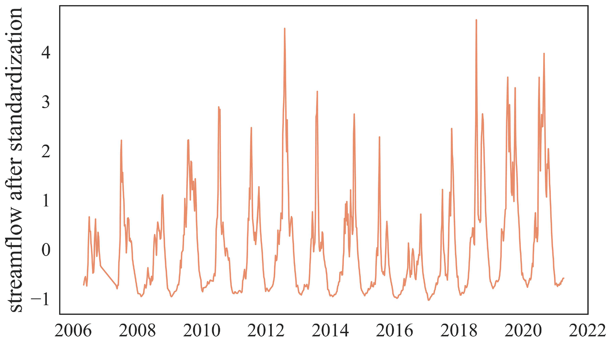
In addition to the basinwise static attributes provided in CCAM, we propose HydroMLYR, a hydrology dataset for machine learning research in the YRB (Fig. 1). HydroMLYR includes standardized streamflow measurements for 102 basins. The streamflow data are 7 d averaged and standardized basinwise to have zero mean and a standard deviation of 1 (Fig. 8). The HydroMLYR dataset is proposed to support machine learning or deep learning hydrology research (e.g., neural-network-based and tree-based algorithms) and can be used in two cases: (i) to develop machine learning models for the YRB or (ii) when it is desirable to verify the generalization ability of a machine learning model for the YRB.
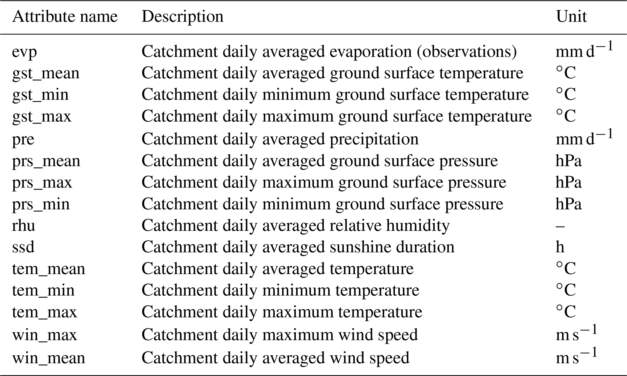
The dataset provides 40 natural basins that are not affected by reservoirs and dams. The selection is based on a newer version (http://globaldamwatch.org/data/#core_global, last access: 26 November 2021) of the Global Reservoirs and Dams database (Lehner et al., 2011), which provides the locations of reservoirs and dams globally. HydroMLYR covers 102 basins in the YRB, including basin boundary shapefiles, static attributes, and standardized streamflow measurements for each basin. The covered basins have areas ranging from 134 to 804 421 km2. Therefore, modeling the YRB on a large scale is also possible. Meteorological records in HydroMLYR introduced daily maxima and minima for some forcing variables (Table 4).
The original streamflow observations are not continuous. The average record length is 11.3 years. Although the development of machine learning models does not necessarily require the data to be continuous, we separately provide continuous streamflow observations with an average record length of 8.3 years.
The proposed dataset is freely available at https://doi.org/10.5281/zenodo.5729444 (Zhen et al., 2021). The files provided are (i) several separate files containing 120+ catchment attributes, (ii) the daily meteorological time series in a zip file, (iii) the catchment boundaries used to compute the attributes and extract the time series, (iv) the HydroMLYR dataset, (v) an attribute description file, and (vi) a readme file. The open-source code (Zhen, 2021) is available at https://github.com/haozhen315/CCAM-China-Catchment-Attributes-and-Meteorology-dataset (last access: 2 December 2021; DOI: https://doi.org/10.5281/zenodo.5749718). It supports generating catchment attributes and meteorological time series for custom catchment boundaries.
The CCAM dataset proposed in this paper provides a novel dataset for hydrological research in China. All basins delaminated from the DEM are studied, covering the whole of China. The dataset includes daily meteorological forcing time series data, including precipitation, temperature, potential evapotranspiration, wind speed, ground surface temperature, pressure, humidity, sunshine duration, and the derived potential evapotranspiration of 4911 catchments. The proposed time series dataset is derived from the quality-controlled SURF_CLI_CHN_MUL_DAY dataset. CCAM includes 120+ catchment attributes, including soil, land cover, geology, climate indices, and topography for each catchment. We produced a series of maps depicting the catchment attribute distributions in China. These maps present regional changes in various features; we also estimated the relationships between them based on Kendall's correlation. Integrating multiple data sources into one dataset at a catchment scale simplifies the data compilation process in research. CCAM can help test hypotheses and formulate valid conclusions under various conditions (i.e., not limited to a few specific locations only) and help explore how different basin characteristics influence hydrological behaviors, learn the migration of hydrological behaviors between different basins, and develop general frameworks for large-scale model evaluation and benchmarking in China. A limitation of this study is its failure to estimate the uncertainty of the meteorological time series. An alternative is to evaluate the uncertainty of the basinwise meteorological data based on multiple independent data sources, but there are few data sources that provide as many data types as SURF_CLI_CHN_MUL_DAY. Hence, evaluating the uncertainty of these eight meteorological variables poses a challenge that is left for future studies.
Penman's equation (Subramanya, 2013), incorporating some modifications to the original formula, is
where PET is the daily potential evapotranspiration in millimeters per day; A is the slope of the saturation vapor pressure (ew) vs. temperature (t) curve at the mean air temperature in millimeters of mercury per degree Celsius; Hn is the net radiation in millimeters of evaporable water per day; Ea is a parameter including wind speed and saturation deficit; and γ is the psychrometric constant equal to 0.49 mm of mercury per degree Celsius.
The relationship between ew and t is defined as follows:
The following equation estimates the net radiation:
where Ha is the incident solar radiation outside the atmosphere on a horizontal surface, expressed in millimeters of evaporable water per day (a function of the latitude and period of the year as indicated in Table B1); a is a constant depending upon the latitude ϕ and is given by a = 0.29 cos ϕ; b is a constant equal to 0.52; n is the sunshine duration in hours; N is the maximum possible hours of bright sunshine (a function of latitude, see Table B2); r is the reflection coefficient; σ is the Stefan–Boltzman constant equal to mm d−1; Ta is the mean air temperature in degrees kelvin; and ea is the actual mean vapor pressure in the air in millimeters of mercury.
Table B1Mean monthly solar radiation, Ha (in mm), of evaporable water per day.
The parameter Ea is estimated as follows:
where u2 is the wind speed at 2 m above ground in kilometers per day; ew is the saturation vapor pressure at mean air temperature in millimeters of mercury; and ea is the actual vapor pressure.
To explore the potential connections between various types of watershed attributes, we performed correlation analysis using the Kendall rank correlation coefficient (Kendall, 1938). The Kendall rank correlation coefficient is a measure of rank correlation: the similarity of the sort order of the two sets of data. Kendall correlation will be high if the orderings of the observations of two variables are similar. Kendall correlation avoids the assumption of a linear relationship and that the distribution should be normal and continuous (e.g., Pearson correlation). When the relationship is not exactly linear, using Pearson correlation will miss out on information that Kendall could capture. Table C1 shows the top five most relevant attributes for each attribute. The analysis result shows that the correlations between variables are in line with general understanding, justifying the rationality of the dataset, and the following names a few:
-
Subsurface permeability and porosity are most correlated with geological attributes.
-
LAI and NDVI are most positively correlated with each other but most negatively correlated with the fraction of barren land cover.
-
Urban and built-up areas are most positively correlated with population density.
-
In China, the savanna is mainly distributed in the southern coastal areas, resulting in it being most positively correlated with mean precipitation.
-
Sand is most positively correlated with saturated hydraulic conductivity, while clay is strongly negatively correlated with saturated hydraulic conductivity.
Table C1The top five most relevant characteristics for each attribute (different soil layers for the same attribute are excluded, e.g., phihox_sl2 is not included in the top five most relevant attributes of phihox_sl1, although they are highly correlated).
The program to generate the dataset is mainly written in Python. The rasterio (https://rasterio.readthedocs.io/en/latest/, last access: 26 November 2021) library is used to extract from the raster for the given basin boundary, reproject, and merge rasters. The shapely (https://shapely.readthedocs.io/en/stable/manual.html, last access: 26 November 2021) library is used to calculate the geometry. The pyproj (https://pyproj4.github.io/pyproj/stable/, last access: 26 November 2021) library is used for coordinate system conversions. The richdem (https://richdem.readthedocs.io/en/latest/, last access: 26 November 2021) library is used to calculate slope. The netCDF4 (https://unidata.github.io/netcdf4-python/, last access: 26 November 2021) and xarray (http://xarray.pydata.org/en/stable/, last access: 26 November 2021, Hoyer et al., 2021) libraries are used to read the netCDF files. The pyshp (https://pypi.org/project/pyshp/, last access: 26 November 2021) library is used to handle shapefiles. The gdal (https://gdal.org , last access: 2 December 2021, GDAL/OGR contributors, 2020) command-line programs are used for data format conversions. The Python multiprocessing (https://docs.python.org/3/library/multiprocessing.html, last access: 26 November 2021) library is used for multithreaded data processing such as the calculation of meteorological time series. The interpolation program is written based on SciPy and NumPy. In addition, the calculation of the catchment boundary uses ArcPy (https://pro.arcgis.com/zh-cn/pro-app/latest/arcpy/get-started/what-is-arcpy-.htm, last access: 26 November 2021). However, ArcPy is not open-source. Upon submission, due to policy adjustments, the SURF_CLI_CHN_MUL_DAY dataset has just been closed for sharing (it may reopen), and we provide two options: (1) calculate time series using the archived SURF_CLI_CHN_MUL_DAY data if there is a backup; and (2) calculate time series using the released CCAM dataset; the principle is to calculate the overlapping areas of the given watershed and the watersheds we have calculated and then to calculate the meteorological time series of the given watersheds by weighting; codes can be found in the GitHub repository. The GDBD dataset can be downloaded at https://www.cger.nies.go.jp/db/gdbd/gdbd_index_e.html (last access: 26 November 2021). ASTER GDEM dataset can be downloaded at https://asterweb.jpl.nasa.gov/gdem.asp (last access: 26 November 2021). The GLHYMPS dataset can be downloaded at https://dataverse.scholarsportal.info/dataset.xhtml?persistentId=doi:10.5683/SP2/DLGXYO (last access: 26 November 2021). MODIS MCD12Q1 can be obtained from https://lpdaac.usgs.gov/products/mcd12q1v006/ (last access: 26 November 2021). MODIS MCD15A3 can be obtained from https://lpdaac.usgs.gov/products/mcd15a3hv006/ (last access: 26 November 2021). Soil hydraulic and thermal properties can be downloaded after registration: http://globalchange.bnu.edu.cn/research/soil5.jsp (last access: 26 November 2021). Soil property data can be downloaded after registration: http://globalchange.bnu.edu.cn/research/soil2 (last access: 26 November 2021). SoilGrids data download link is https://files.isric.org/soilgrids/former/2017-03-10/data/ (last access: 26 November 2021) with a list of descriptions at https://github.com/ISRICWorldSoil/SoilGrids250m/blob/master/grids/models/META_GEOTIFF_1B.csv (last access: 26 November 2021).
This section briefly introduces how the basin boundaries are derived. The basin boundary data used in this research are obtained from the GBDB (Global Drainage Basin Database; Masutomi et al., 2009) dataset. The GDBD dataset first distinguishes sinks caused by DEM errors; then, stream burning (Maidment, 1996) and ridge fencing methods are used to modify the seeded DEM, and basin boundaries are produced with standardized procedures (Jenson and Domingue, 1988; Maidment and Morehouse, 2002). Then, the gauging station data from the GRDC dataset are used to calibrate the derived basin boundaries. The derived basin areas were compared with the observed basin areas, and they showed a high degree of consistency with the observed basin data.
The published code (https://github.com/haozhen315/CCAM-China-Catchment-Attributes-and-Meteorology-dataset, last access: 26 November 2021) supports the automation of the calculation of the attributes for any given river basin and the generation of statistics files. In general, the user only needs to prepare the source data and ensure that the code environment is installed correctly, and then the user can run the code to calculate all attributes for the given river basin. The following describes the steps to generate data for any given watershed.
F1 Prepare source data
In this step, the user needs to download the source data and place it in the corresponding location (Table F1). The code supports the calculation of meteorological time series based on the SURF_CLI_CHN_MUL_DAY dataset or the CCAM dataset that we have released. If the basin the user needs to calculate is not in China, then the user needs to format the collected meteorological time series into the same format as the time series generated by the code. Details and sample files are available in the GitHub library.
Table F1Instructions for preparing data sources.
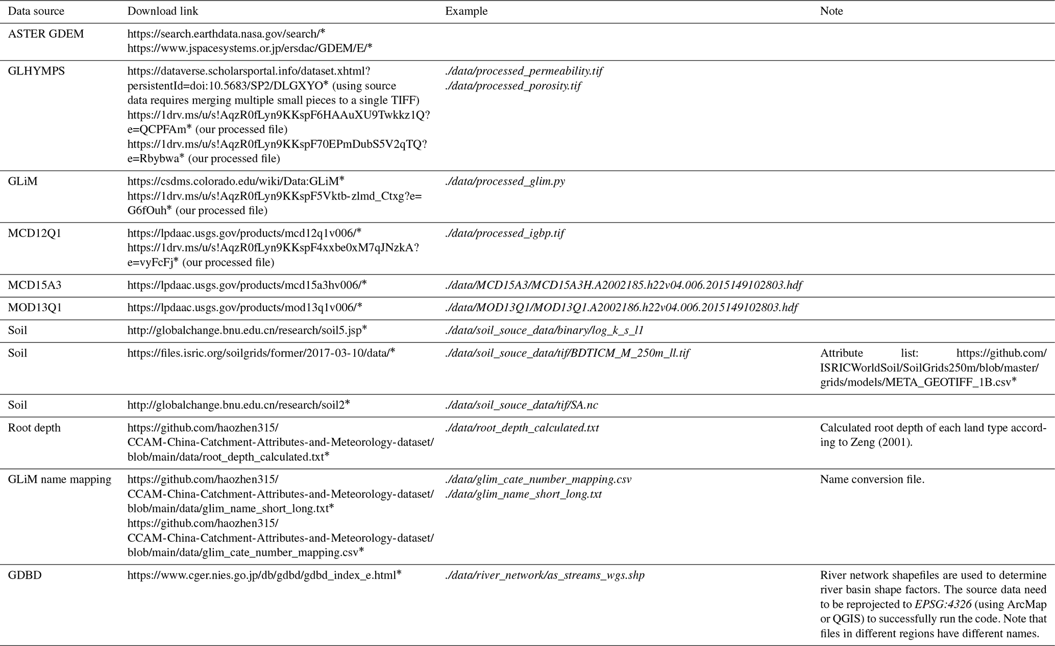
* last access: 26 November 2021.
F2 Run the code
When all the source data are prepared, the user can run the code calculate_all_attributes.py to calculate all attributes or run separate scripts (e.g., soil.py) to calculate indicators for specific categories. The result will appear in the output folder.
ZH was responsible for data curation, software, analysis, investigation, methodology, validation, visualization, writing the original draft, review, and editing. JJ was responsible for conceptualization, methodology, formal analysis, writing, review, editing, project administration, supervision, and funding acquisition. RX was responsible for supervision, formal analysis, writing, review, and editing. ST, WY, QL, and MZ were responsible for formal analysis, writing, review, and editing. TM and CJ were responsible for investigation and data curation. YZ was responsible for conceptualization and supervision.
The contact author has declared that neither they nor their co-authors have any competing interests.
Publisher's note: Copernicus Publications remains neutral with regard to jurisdictional claims in published maps and institutional affiliations.
This research was supported by the National Key Research and Development Program (grant nos. 2018YFC0407901 and 2018YFC0407905), the National Natural Science Fund of China (grant no. 51779100), and the Central Public-interest Scientific Institution Basal Research Fund (grant nos. HKY-JBYW-2020-21, HKY-JBYW-2020-07, and HKY- JBYW-2021-02).
This paper was edited by Lukas Gudmundsson and reviewed by two anonymous referees.
Abrams, M., Crippen, R., and Fujisada, H.: ASTER global digital elevation model (GDEM) and ASTER global water body dataset (ASTWBD), Remote Sensing, 12, 1156, https://doi.org/10.3390/rs12071156, 2020.
Addor, N., Newman, A. J., Mizukami, N., and Clark, M. P.: The CAMELS data set: catchment attributes and meteorology for large-sample studies, Hydrol. Earth Syst. Sci., 21, 5293–5313, https://doi.org/10.5194/hess-21-5293-2017, 2017.
Addor, N., Do, H. X., Alvarez-Garreton, C., Coxon, G., Fowler, K., and Mendoza, P. A.: Large-sample hydrology: recent progress, guidelines for new datasets and grand challenges, Hydrolog. Sci. J., 65, 712–725, 2020.
Alvarez-Garreton, C., Mendoza, P. A., Boisier, J. P., Addor, N., Galleguillos, M., Zambrano-Bigiarini, M., Lara, A., Puelma, C., Cortes, G., Garreaud, R., McPhee, J., and Ayala, A.: The CAMELS-CL dataset: catchment attributes and meteorology for large sample studies – Chile dataset, Hydrol. Earth Syst. Sci., 22, 5817–5846, https://doi.org/10.5194/hess-22-5817-2018, 2018.
Belward, A. S., Estes, J. E., and Kline, K. D.: The IGBP-DIS global 1-km land-cover data set DISCover: A project overview, Photogramm. Eng. Rem. S., 65, 1013–1020, 1999.
Berghuijs, W. R., Aalbers, E. E., Larsen, J. R., Trancoso, R., and Woods, R. A.: Recent changes in extreme floods across multiple continents, Environ. Res. Lett., 12, 114035, https://doi.org/10.1088/1748-9326/aa8847, 2017.
Blume, T., van Meerveld, I., and Weiler, M.: Incentives for field hydrology and data sharing: collaboration and compensation: reply to “A need for incentivizing field hydrology, especially in an era of open data”, Hydrolog. Sci. J., 63, 1266–1268, 2018.
Brodeur, Z. P., Herman, J. D., and Steinschneider, S.: Bootstrap Aggregation and Cross-Validation Methods to Reduce Overfitting in Reservoir Control Policy Search, Water Resour. Res., 56, e2020WR027184, https://doi.org/10.1029/2020WR027184, 2020.
Buermann, W., Dong, J., Zeng, X., Myneni, R. B., and Dickinson, R. E.: Evaluation of the utility of satellite-based vegetation leaf area index data for climate simulations, J. Climate, 14, 3536–3550, 2001.
Bureau of Geology and Mineral Resources of Xinjiang (BGX): Geological map of Xinjiang Uygur, Autonomous Region, China, version 2, scale , Geol. Publ. House, Beijing, 1992.
Ceola, S., Arheimer, B., Baratti, E., Blöschl, G., Capell, R., Castellarin, A., Freer, J., Han, D., Hrachowitz, M., Hundecha, Y., Hutton, C., Lindström, G., Montanari, A., Nijzink, R., Parajka, J., Toth, E., Viglione, A., and Wagener, T.: Virtual laboratories: new opportunities for collaborative water science, Hydrol. Earth Syst. Sci., 19, 2101–2117, https://doi.org/10.5194/hess-19-2101-2015, 2015.
Chagas, V. B. P., Chaffe, P. L. B., Addor, N., Fan, F. M., Fleischmann, A. S., Paiva, R. C. D., and Siqueira, V. A.: CAMELS-BR: hydrometeorological time series and landscape attributes for 897 catchments in Brazil, Earth Syst. Sci. Data, 12, 2075–2096, https://doi.org/10.5194/essd-12-2075-2020, 2020.
China Geological Survey (CGS): -scale digital geological map database of China, Beijing, 2001.
Coron, L., Andreassian, V., Perrin, C., Lerat, J., Vaze, J., Bourqui, M., and Hendrickx, F.: Crash testing hydrological models in contrasted climate conditions: An experiment on 216 Australian catchments, Water Resour. Res., 48, W05552, https://doi.org/10.1029/2011WR011721, 2012.
Coxon, G., Addor, N., Bloomfield, J. P., Freer, J., Fry, M., Hannaford, J., Howden, N. J. K., Lane, R., Lewis, M., Robinson, E. L., Wagener, T., and Woods, R.: CAMELS-GB: hydrometeorological time series and landscape attributes for 671 catchments in Great Britain, Earth Syst. Sci. Data, 12, 2459–2483, https://doi.org/10.5194/essd-12-2459-2020, 2020.
Dai, Y., Xin, Q., Wei, N., Zhang, Y., Shangguan, W., Yuan, H., Zhang, S., Liu, S., and Lu, X.: A global high-resolution data set of soil hydraulic and thermal properties for land surface modeling, J. Adv. Model. Earth Sy., 11, 2996–3023, 2019.
de Araújo, J. C. and González Piedra, J. I.: Comparative hydrology: analysis of a semiarid and a humid tropical watershed, Hydrol. Process., 23, 1169–1178, 2009.
Desborough, C. E.: The impact of root weighting on the response of transpiration to moisture stress in land surface schemes, Mon. Weather Rev., 125, 1920–1930, 1997.
Didan, K.: MOD13A3 MODIS/Terra vegetation Indices Monthly L3 Global 1km SIN Grid V006, NASA EOSDIS Land Processes DAAC [Data set], https://doi.org/10.5067/MODIS/MOD13A3.006, 2015.
Feng, D., Fang, K., and Shen, C.: Enhancing streamflow forecast and extracting insights using long-short term memory networks with data integration at continental scales, Water Resour. Res., 56, e2019WR026793, https://doi.org/10.1029/2019WR026793, 2020.
Friedl, M. A., Sulla-Menashe, D., Tan, B., Schneider, A., Ramankutty, N., Sibley, A., and Huang, X.: MODIS Collection 5 global land cover: Algorithm refinements and characterization of new datasets, Remote Sens. Environ., 114, 168–182, 2010.
GDAL/OGR contributors: GDAL/OGR Geospatial Data Abstraction software Library, Open Source Geospatial Foundation [code], available at: https://gdal.org (last access: 26 November 2021), 2020.
Gleeson, T., Smith, L., Moosdorf, N., Hartmann, J., Dürr, H. H., Manning, A. H., van Beek, L. P., and Jellinek, A. M.: Mapping permeability over the surface of the Earth, Geophys. Res. Lett., 38, L02401, https://doi.org/10.1029/2010GL045565, 2011.
Gleeson, T., Moosdorf, N., Hartmann, J., and Van Beek, L.: A glimpse beneath earth's surface: GLobal HYdrogeology MaPS (GLHYMPS) of permeability and porosity, Geophys. Res. Lett., 41, 3891–3898, 2014.
Gudmundsson, L., Leonard, M., Do, H. X., Westra, S., and Seneviratne, S. I.: Observed trends in global indicators of mean and extreme streamflow, Geophys. Res. Lett., 46, 756–766, 2019.
Hartmann, J. and Moosdorf, N.: The new global lithological map database GLiM: A representation of rock properties at the Earth surface, Geochem. Geophy. Geosy., 13, Q12004, https://doi.org/10.1029/2012GC004370, 2012.
Hengl, T., Mendes de Jesus, J., Heuvelink, G. B., Ruiperez Gonzalez, M., Kilibarda, M., Blagotić, A., Shangguan, W., Wright, M. N., Geng, X., and Bauer-Marschallinger, B.: SoilGrids250m: Global gridded soil information based on machine learning, PLoS one, 12, e0169748, https://doi.org/10.1371/journal.pone.0169748, 2017.
Horn, B. K.: Hill shading and the reflectance map, Proc. IEEE, 69, 14–47, 1981.
Hoyer, S. and Hamman, J.: xarray: ND labeled arrays and datasets in Python, Journal of Open Research Software [code], 5, 2017.
Huang, H., Han, Y., Cao, M., Song, J., and Xiao, H.: Spatial-temporal variation of aridity index of China during 1960–2013, Adv. Meteorol., 2016, 1536135, https://doi.org/10.1155/2016/1536135, 2016.
Jenson, S. K. and Domingue, J. O.: Extracting topographic structure from digital elevation data for geographic information system analysis, Photogramm. Eng. Rem. S., 54, 1593–1600, 1988.
Kendall, M. G.: A new measure of rank correlation, Biometrika, 30, 81–93, 1938.
Knoben, W. J. M., Freer, J. E., and Woods, R. A.: Technical note: Inherent benchmark or not? Comparing Nash–Sutcliffe and Kling–Gupta efficiency scores, Hydrol. Earth Syst. Sci., 23, 4323–4331, https://doi.org/10.5194/hess-23-4323-2019, 2019.
Knyazikhin, Y.: MODIS leaf area index (LAI) and fraction of photosynthetically active radiation absorbed by vegetation (FPAR) product (MOD 15) algorithm theoretical basis document, available at: https://modis.gsfc.nasa.gov/data/atbd/atbd_mod15.pdf (last access: 26 November 2021), 1999.
Kollat, J., Reed, P., and Wagener, T.: When are multiobjective calibration trade-offs in hydrologic models meaningful?, Water Resour. Res., 48, W03520, https://doi.org/10.1029/2011WR011534, 2012.
Kratzert, F., Klotz, D., Shalev, G., Klambauer, G., Hochreiter, S., and Nearing, G.: Towards learning universal, regional, and local hydrological behaviors via machine learning applied to large-sample datasets, Hydrol. Earth Syst. Sci., 23, 5089–5110, https://doi.org/10.5194/hess-23-5089-2019, 2019.
Lane, R. A., Coxon, G., Freer, J. E., Wagener, T., Johnes, P. J., Bloomfield, J. P., Greene, S., Macleod, C. J. A., and Reaney, S. M.: Benchmarking the predictive capability of hydrological models for river flow and flood peak predictions across over 1000 catchments in Great Britain, Hydrol. Earth Syst. Sci., 23, 4011–4032, https://doi.org/10.5194/hess-23-4011-2019, 2019.
Legasa, M. and Gutiérrez, J. M.: Multisite Weather Generators using Bayesian Networks: An illustrative case study for precipitation occurrence, Water Resour. Res., 56, e2019WR026416, https://doi.org/10.1029/2019WR026416, 2020.
Lehner, B.: HydroBASINS: Global watershed boundaries and sub-basin delineations derived from HydroSHEDS data at 15 second resolution – Technical documentation version 1. c, 2014.
Lehner, B., Verdin, K., and Jarvis, A: New global hydrography derived from spaceborne elevation data, Eos, Transactions, AGU, 89, 93–94, 2008.
Lehner, B., Liermann, C. R., Revenga, C., Vörösmarty, C., Fekete, B., Crouzet, P., Döll, P., Endejan, M., Frenken, K., and Magome, J.: Global reservoir and dam (grand) database, Technical Documentation, Version, 1, 1–14, 2011.
Linke, S., Lehner, B., Dallaire, C. O., Ariwi, J., Grill, G., Anand, M., Beames, P., Burchard-Levine, V., Maxwell, S., and Moidu, H.: Global hydro-environmental sub-basin and river reach characteristics at high spatial resolution, Sci. Data, 6, 1–15, 2019.
Liu, B., Xu, M., Henderson, M., and Gong, W.: A spatial analysis of pan evaporation trends in China, 1955–2000, J. Geophys. Res.-Atmos., 109, D15102, https://doi.org/10.1029/2004JD004511, 2004.
Liu, Q., Yang, Z., and Xia, X.: Trends for pan evaporation during 1959–2000 in China, Procedia Environ. Sci., 2, 1934–1941, 2010.
Liu, Y., Zheng, J., Hao, Z., and Zhang, X.: Unprecedented warming revealed from multi-proxy reconstruction of temperature in southern China for the past 160 years, Adv. Atmos. Sci., 34, 977–982, 2017.
Maidment, D. R.: GIS and hydrologic modeling-an assessment of progress, Third International Conference on GIS and Environmental Modeling, Santa Fe, New Mexico, 1996.
Maidment, D. R. and Morehouse, S.: Arc Hydro: GIS for water resources, ESRI Press, Redlands, CA, USA, 2002.
Masutomi, Y., Inui, Y., Takahashi, K., and Matsuoka, Y.: Development of highly accurate global polygonal drainage basin data, Hydrol. Process., 23, 572–584, 2009.
Mei, Y., Maggioni, V., Houser, P., Xue, Y., and Rouf, T.: A nonparametric statistical technique for spatial downscaling of precipitation over High Mountain Asia, Water Resour. Res., 56, e2020WR027472, https://doi.org/10.1029/2020WR027472, 2020.
Ministry of Geology and Mineral Resources of the People’s Republic of China (MGC): Geological map of Nei Mongol Autonomous Region, People’s Republic of China, scale , Geol. Publ. House, Beijing, 1991.
Myneni, R., Knyazikhin, Y., and Park, T.: MYD15A2H MODIS/Aqua Leaf Area Index/FPAR 8-Day L4 Global 500m SIN Grid, Boston University and MODAPS SIPS – NASA, NASA LP DAAC [dataset], https://doi.org/10.5067/MODIS/MYD15A2H.006 2015.
Nevo, S., Anisimov, V., Elidan, G., El-Yaniv, R., Giencke, P., Gigi, Y., Hassidim, A., Moshe, Z., Schlesinger, M., and Shalev, G.: ML for flood forecasting at scale, arXiv [preprint], arXiv:1901.09583, 2019.
Newman, A. J., Clark, M. P., Sampson, K., Wood, A., Hay, L. E., Bock, A., Viger, R. J., Blodgett, D., Brekke, L., Arnold, J. R., Hopson, T., and Duan, Q.: Development of a large-sample watershed-scale hydrometeorological data set for the contiguous USA: data set characteristics and assessment of regional variability in hydrologic model performance, Hydrol. Earth Syst. Sci., 19, 209–223, https://doi.org/10.5194/hess-19-209-2015, 2015.
Ni, H. and Benson, S. M.: Using Unsupervised Machine Learning to Characterize Capillary Flow and Residual Trapping, Water Resour. Res., 56, e2020WR027473, https://doi.org/10.1029/2020WR027473, 2020.
Oudin, L., Andréassian, V., Lerat, J., and Michel, C.: Has land cover a significant impact on mean annual streamflow? An international assessment using 1508 catchments, J. Hydrol., 357, 303–316, 2008.
Running, S. and Mu, Q.: MOD16A2 MODIS/Terra Evapotranspiration 8-day L4 Global 500m SIN Grid, University of Montana and MODAPS SIPS – NASA, NASA LP DAAC [data set], https://doi.org/10.5067/MODIS/MOD16A2.006, 2017.
Seybold, H., Rothman, D. H., and Kirchner, J. W.: Climate's watermark in the geometry of stream networks, Geophys. Res. Lett., 44, 2272–2280, 2017.
Shangguan, W., Dai, Y., Liu, B., Zhu, A., Duan, Q., Wu, L., Ji, D., Ye, A., Yuan, H., and Zhang, Q.: A China data set of soil properties for land surface modeling, J. Adv. Model. Earth Sy., 5, 212–224, 2013.
Shangguan, W., Dai, Y., Duan, Q., Liu, B., and Yuan, H.: A global soil data set for earth system modeling, J. Adv. Model. Earth Sy., 6, 249–263, 2014.
Shen, C., Laloy, E., Elshorbagy, A., Albert, A., Bales, J., Chang, F.-J., Ganguly, S., Hsu, K.-L., Kifer, D., Fang, Z., Fang, K., Li, D., Li, X., and Tsai, W.-P.: HESS Opinions: Incubating deep-learning-powered hydrologic science advances as a community, Hydrol. Earth Syst. Sci., 22, 5639–5656, https://doi.org/10.5194/hess-22-5639-2018, 2018.
Silberstein, R.: Hydrological models are so good, do we still need data?, Environ. Model. Softw., 21, 1340–1352, 2006.
Singh, R., Archfield, S., and Wagener, T.: Identifying dominant controls on hydrologic parameter transfer from gauged to ungauged catchments – A comparative hydrology approach, J. Hydrol., 517, 985–996, 2014a.
Singh, R., van Werkhoven, K., and Wagener, T.: Hydrological impacts of climate change in gauged and ungauged watersheds of the Olifants basin: a trading-space-for-time approach, Hydrolog. Sci. J., 59, 29–55, 2014b.
Subramanya, K.: Engineering Hydrology, 4e, McGraw Hill Education Private Limited P-24, Green Park Extension, New Delhi, India, 2013.
Sulla-Menashe, D. and Friedl, M. A.: User guide to collection 6 MODIS land cover (MCD12Q1 and MCD12C1) product, USGS, Reston, VA, USA, 1–18, 2018.
Tyralis, H., Papacharalampous, G., and Tantanee, S.: How to explain and predict the shape parameter of the generalized extreme value distribution of streamflow extremes using a big dataset, J. Hydrol., 574, 628–645, 2019.
van Werkhoven, K., Wagener, T., Reed, P., and Tang, Y.: Characterization of watershed model behavior across a hydroclimatic gradient, Water Resour. Res., 44, W01429, https://doi.org/10.1029/2007WR006271, 2008.
van Wijk, M. T. and Williams, M.: Optical instruments for measuring leaf area index in low vegetation: application in arctic ecosystems, Ecol. Appl., 15, 1462–1470, 2005.
Voepel, H., Ruddell, B., Schumer, R., Troch, P. A., Brooks, P. D., Neal, A., Durcik, M., and Sivapalan, M.: Quantifying the role of climate and landscape characteristics on hydrologic partitioning and vegetation response, Water Resour. Res., 47, W00J09, https://doi.org/10.1029/2010WR009944, 2011.
Wang, J., Chen, M., Lü, G., Yue, S., Wen, Y., Lan, Z., and Zhang, S.: A data sharing method in the open web environment: Data sharing in hydrology, J. Hydrol., 587, 124973, https://doi.org/10.1016/j.jhydrol.2020.124973, 2020.
Wongso, E., Nateghi, R., Zaitchik, B., Quiring, S., and Kumar, R.: A Data-Driven Framework to Characterize State-Level Water Use in the United States, Water Resour. Res., 56, e2019WR024894, https://doi.org/10.1029/2019WR024894, 2020.
Woods, R. A.: Analytical model of seasonal climate impacts on snow hydrology: Continuous snowpacks, Adv. Water Resour., 32, 1465–1481, 2009.
Xu, Y., Gao, X., Shen, Y., Xu, C., Shi, Y., and Giorgi, a.: A daily temperature dataset over China and its application in validating a RCM simulation, Adv. Atmos. Sci., 26, 763–772, 2009.
Yamazaki, D., Ikeshima, D., Sosa, J., Bates, P. D., Allen, G. H., and Pavelsky, T. M.: MERIT Hydro: a high-resolution global hydrography map based on latest topography dataset, Water Resour. Res., 55, 5053–5073, 2019.
Zeng, X.: Global vegetation root distribution for land modeling, J. Hydrometeorol., 2, 525–530, 2001.
Zhen, H.: CCAM: China Catchment Attributes and Meteorology dataset, Zenodo [code], https://doi.org/10.5281/zenodo.5749718, last access: 30 November 2021.
Zhen, H., Jin, J., Xia, R., Tian, S., Yang, W., Liu, Q., Zhu, M., Ma, T., and Chengran, J.: CCAM: China Catchment Attributes and Meteorology dataset, Zenodo [data set], https://doi.org/10.5281/zenodo.5729444, 2021.
- Abstract
- Introduction
- Study area
- Climatic indices
- Geology
- Land cover
- Location and topography
- Soil
- Meteorological time series
- HydroMLYR: hydrology dataset for machine learning in YRB
- Code and data availability
- Conclusions
- Appendix A: Attributes summary
- Appendix B: Modified Penman's equation
- Appendix C: Correlation analysis of catchment attributes
- Appendix D: Data sources and processing
- Appendix E: Basin boundaries
- Appendix F: Guidelines for calculating attributes for custom catchments
- Author contributions
- Competing interests
- Disclaimer
- Financial support
- Review statement
- References