the Creative Commons Attribution 4.0 License.
the Creative Commons Attribution 4.0 License.
 | 01 Dec 2021
EUREC4A's HALO
Florian Ewald
Geet George
Marek Jacob
Marcus Klingebiel
Tobias Kölling
Anna E. Luebke
Theresa Mieslinger
Veronika Pörtge
Jule Radtke
Michael Schäfer
Hauke Schulz
Raphaela Vogel
Martin Wirth
Sandrine Bony
Susanne Crewell
André Ehrlich
Linda Forster
Andreas Giez
Felix Gödde
Silke Groß
Manuel Gutleben
Martin Hagen
Lutz Hirsch
Friedhelm Jansen
Theresa Lang
Bernhard Mayer
Mario Mech
Marc Prange
Sabrina Schnitt
Jessica Vial
Andreas Walbröl
Manfred Wendisch
Kevin Wolf
Tobias Zinner
Martin Zöger
Felix Ament
Bjorn Stevens
As part of the EUREC4A (Elucidating the role of cloud–circulation coupling in climate) field campaign, the German research aircraft HALO (High Altitude and Long Range Research Aircraft), configured as a cloud observatory, conducted 15 research flights in the trade-wind region east of Barbados in January and February 2020. Narrative text, aircraft state data, and metadata describing HALO's operation during the campaign are provided. Each HALO research flight is segmented by timestamp intervals into standard elements to aid the consistent analysis of the flight data. Photographs from HALO's cabin and animated satellite images synchronized with flight tracks are provided to visually document flight conditions. As a comprehensive product from the remote sensing observations, a multi-sensor cloud mask product is derived and quantifies the incidence of clouds observed during the flights. In addition, to lower the threshold for new users of HALO's data, a collection of use cases is compiled into an online book, How to EUREC4A, included as an asset with this paper. This online book provides easy access to most of EUREC4A's HALO data through an intake catalogue. Code and data are freely available at the locations specified in Table 6.
- Article
(12290 KB) - Full-text XML
-
Supplement
(8004 KB) - BibTeX
- EndNote


The EUREC4A (Elucidating the role of cloud–circulation coupling in climate; Bony et al., 2017) field campaign took advantage of the capabilities of the cloud-observatory configuration of the German research aircraft HALO (High Altitude and Long Range Research Aircraft; Krautstrunk and Giez, 2012). This configuration, as described by Stevens et al. (2019), was developed and implemented over the course of several previous HALO campaigns, two of which – NARVAL South (Klepp et al., 2014) and NARVAL2 (NARVAL stands for Next-generation Advanced Remote sensing for VALidation; Stevens et al., 2020) based out of Barbados – were in direct preparation for EUREC4A. As motivated by Bony et al. (2017) and described by Stevens et al. (2021), EUREC4A made measurements to (i) test hypothesized mechanisms that would cause large reductions in trade-wind cloudiness with warming and (ii) benchmark a new generation of global storm-resolving models (Satoh et al., 2019).
HALO was one of four scientific platforms forming the nucleus of EUREC4A. Its measurements were closely coordinated with those from the other three core platforms – the research vessel (R/V) Meteor, the Barbados Cloud Observatory (BCO; Stevens et al., 2016), and the French SAFIRE ATR 42 – to facilitate observations of the same air mass from different vantage points. Two additional aircraft, three further research vessels, and a small fleet of air- and water-borne robotic instrument platforms supported a substantial broadening of EUREC4A's initial scope and, as described by Stevens et al. (2021), involved looser coordination with HALO. Often the day-to-day operation time and area of these platforms were not closely matched with the platforms mentioned above, but these platforms were still operated in the general EUREC4A area during the campaign period and coordinated measurements were still conducted from time to time. In this paper we elaborate on HALO's contribution to EUREC4A, independent of the other platforms. We do so by describing how HALO was deployed during EUREC4A, both in standard narrative form and through the provision of auxiliary data and metadata, including flight segmentation data, animated geostationary satellite data with flight tracks, and curated photographs (Sect. 2). Through the provision of aircraft state information and the construction of a multi-sensor cloud mask product, Sect. 3 gives a synthetic overview of HALO's scientific payload and the varying cloud conditions it observed. Section 4 outlines how to access and use the HALO measurements as part of a developing data concept. Links to the data and a brief summary are provided in Sect. 6.
HALO is a Gulfstream G550 that has been modified for atmospheric research and is operated by the German Aerospace Center (Krautstrunk and Giez, 2012; Wendisch et al., 2016). During EUREC4A HALO was flown in a slightly updated version of the cloud-observatory configuration described by Stevens et al. (2019). In addition to housekeeping data (aircraft state and in situ meteorological measurements), this updated configuration consists of a nadir-looking differential absorption and high-spectral-resolution lidar (Wirth et al., 2009), a cloud radar and microwave radiometer (Mech et al., 2014), a zenith-oriented spectral radiometer (Wendisch et al., 2001), an imaging spectrometer (Ewald et al., 2016), a thermal imaging polarimeter, an infrared imager, a dropsonde system, and broadband radiometers. The imaging polarimeter, infrared imager, and broadband radiometers were new additions to the HALO cloud-observatory configuration. In this section we describe how and where HALO was deployed. This description is aided by the development of a metadata concept (and the metadata arising from its application) to systematically segment the flight data and document the meteorological conditions (through photographs and satellite imagery) encountered on the different flights.
2.1 Flights
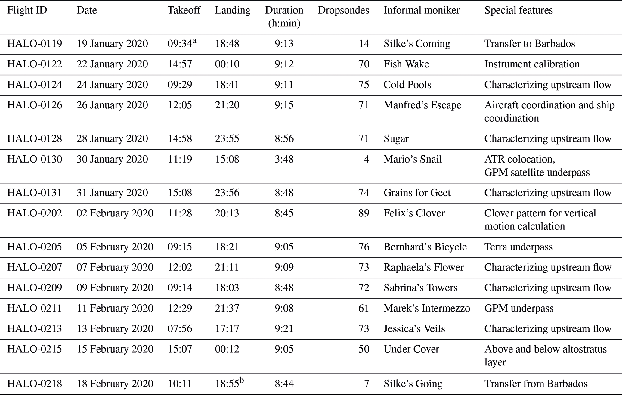
HALO performed 15 research flights on 15 different days in support of EUREC4A, as listed (with an evocative moniker) in Table 1. Flight IDs in the format HALO-MMDD (where M is month and D is day), rather than an enumeration of the research flights, are used to distinguish the different flights. This helps avoid confusion arising from non-coincident flights among the various research aircraft contributing to EUREC4A. Of these, 13 (HALO-0122 to HALO-0215) are designated as local flights, as they had both the takeoff and landing at Barbados' Grantley Adams International Airport. With the exception of HALO-0130 – a short flight that took advantage of overlap in crew duty to make some additional measurements of opportunity – each local flight lasted about 9 h, with roughly 7 h of circling on what Stevens et al. (2021) call the “EUREC4A-Circle”. This circle was largely defined by the HALO flight pattern, which was fixed before the beginning of the campaign to support the deployment of dropsondes around a geographically fixed circle positioned windward of the BCO (Barbados Cloud Observatory; Stevens et al., 2016), far enough upwind to not interfere with commercial air traffic but not so far as to be out of range of a C-band polarized research radar (POLDIRAD). The EUREC4A-Circle is easily identified as the darkest circle area in the heat map of flight tracks in Fig. 1, with a center at 13.3∘ N, 57.717∘ W and an approximately 220 km diameter.
Table 1HALO research flights during EUREC4A. Except for HALO-0119 and HALO-0218, all flights were local flights that took off and landed at Grantley Adams International Airport on Barbados. All times are given as UTC. The special features column gives information about the purpose of each flight aside from the EUREC4A-Circle pattern.
a Takeoff at Santiago de Compostela Airport, Spain. b Landing at Oberpfaffenhofen Airport, Germany.
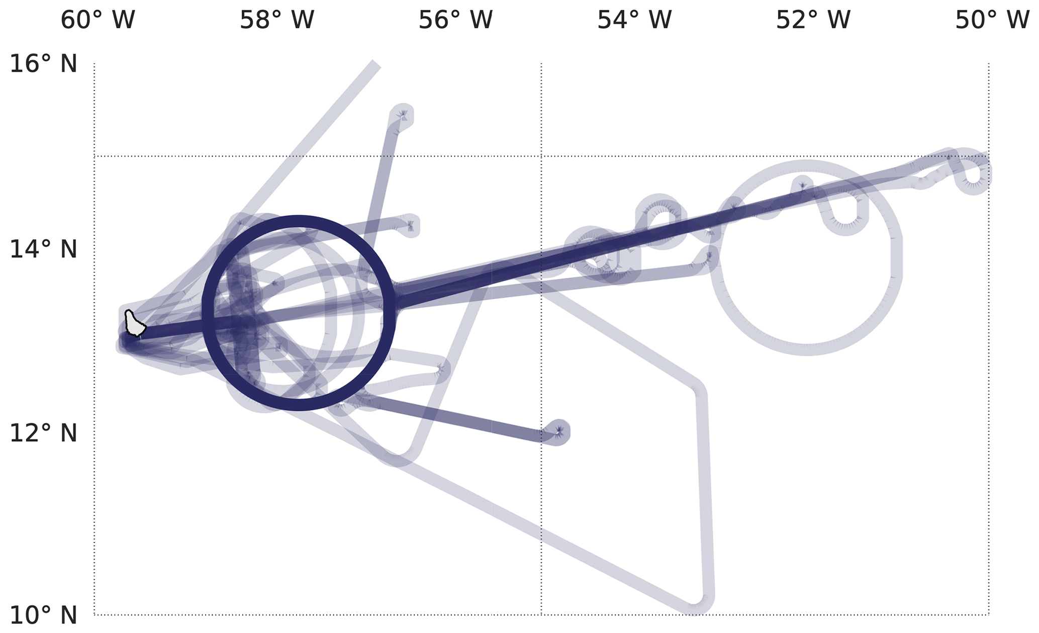
Figure 1Heat map of HALO flight tracks from all 15 flights. The darkness of the color represents the frequency a location was visited. Map data based on Wessel and Smith (1996).
An important and unusual aspect of the HALO (and EUREC4A) flight strategy was that it did not target specific meteorological conditions. Flight days were scheduled in coordination with the ATR aircraft so as to maximize the utilization of the aircraft subject to crew duty restrictions. Variations in takeoff (and landing) times were implemented to better sample the diurnal cycle and were staggered to accommodate crew duty considerations, rather than to target specific meteorological conditions. On most flights some time was also dedicated to flight elements other than the EUREC4A-Circle, for instance to allow an underpass of a meteorological satellite (e.g., the Terra satellite during Bernhard's Bicycle) or to sample the upwind conditions that were being monitored by other platforms. Only Mario's Snail (HALO-0130); the southeast excursion on Manfred's Escape (HALO-0126), which coordinated sampling of a cirrus deck with the R/V Meteor; and the choice of flight levels on Under Cover were influenced by meteorological conditions. The moniker associated with each flight (Table 1) was chosen to strengthen the mental image associated with that flight and in most cases remind the reader of the principle investigator (PI) of each flight.
2.2 Flight segmentation
To aid in the analysis of flight data, all HALO flights are segmented via timestamps into a system of hierarchical identifiers. Non-exclusive segments are defined by two (YYYY-MM-DD hh:mm:ss) timestamps, the first one defining the start of the segment and the second denoting the first time step after the end of the segment. Timestamps have a temporal resolution of 1 s, and times are given in UTC. Every segment belongs to a “kind” – a categorical type for segments defined in Table 2. It helps to think of segments as an interval of flight time and the corresponding kinds as describing how the aircraft was being operated during this time interval (Fig. 2).
Figure 2Examples of flight segments (colored) for two research flights: (a) on flight HALO-0131 and (b) on flight HALO-0202. Portions of flight track that are not segmented appear as dotted lines. Map data based on Wessel and Smith (1996).
Flight segmentation data are provided as YAML (YAML Ain't Markup Language) files that can be accessed at https://doi.org/10.5281/zenodo.4900003. This section provides a description of the YAML files and the reasoning behind their structure and method.
Table 2Definition of flight segments. The total number of these segments identified from all flights has been provided in the rightmost column.

By adopting non-exclusive segments, a timestamp can belong to multiple segments that differ in kind. For example, timestamps belonging to the kind “lidar leg” will also belong to the kind “straight leg” if they match the definition of the latter. Segment start and end times were first roughly categorized based on timestamps from the flight reports and aircraft navigation features such as roll angle, altitude, pitch, etc. However, the final attribution of timestamps to segments was performed manually by the listed contact in the YAML files. At least one other person later tested the segmentation for errors or avoidable deviations from the segment definitions (Table 2). This was done to maintain the objective segment classification whenever possible so that the user of these data can expect the segments to match the definition as closely as possible. As the segmentation was performed manually, segments are defined by the time intervals that are assigned to them, rather than by their kind.
The flight segments in the YAML files also contain a field called “dropsondes”, which provides a list of the dropsondes, whose times of launch are associated with the respective segment. The dropsondes are provided with classifications of good, bad, and ugly, based on their QC classification types from the EUREC4A dropsonde dataset JOANNE (Joint dropsonde Observations of the Atmosphere in tropical North atlaNtic meso-scale Environments; George et al., 2021). The list is in the form of unique dropsonde IDs that correspond to the variable “sonde_id” provided in JOANNE and are the “cf_role” variable therein. This field makes it convenient for selection of the dropsondes based on flight segments. In a few instances the launch time of a dropsonde will fall outside of the segment with which it is associated – for instance if the last sonde of a circle was inadvertently launched too late, after HALO had completed a circle.
Table 3List of standard irregularities attributed to flight segments.
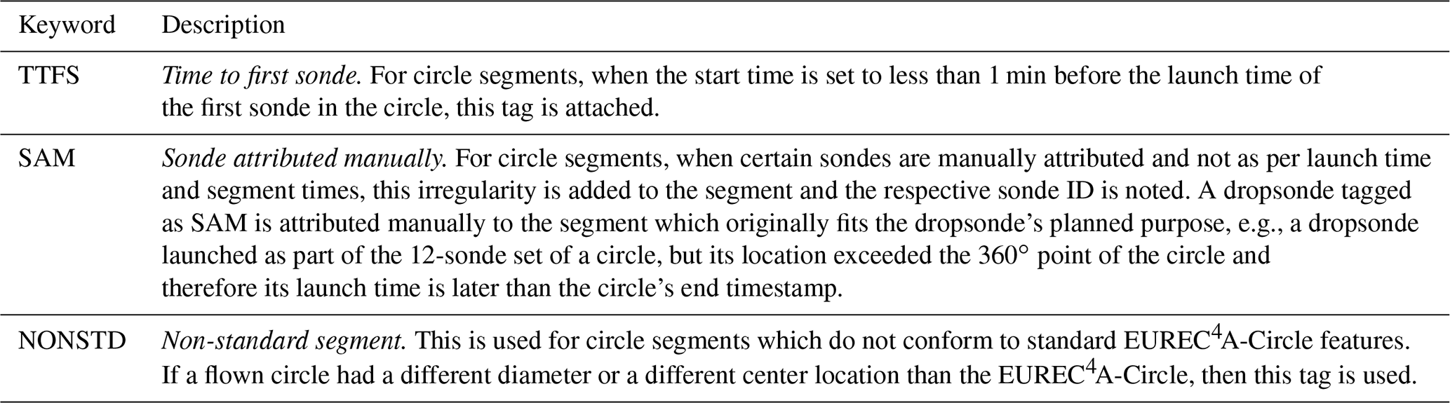
Flight segments that deviated from the allowed kinds are flagged by an irregularity field. For instance, the inclusion of sondes launched before or after their associated flight segment constitutes an irregularity and is marked. The irregularity field takes the form of an explanatory string describing the irregularity. As the segmentation process revealed some oft-repeated irregularities, standardized irregularity tags (keywords) were defined (Table 3) and are prepended to the explanatory string of the irregularity field when applicable.
In total 220 segments were defined over the 15 flights. These included 72 circles (69 regular, 1 with a smaller diameter, 1 outside of the EUREC4A-Circle, and 1 without dropsonde launches) within 26 periods of circling. Fifty-one straight legs were flown. The segmentation data are published by Prange et al. (2021).
2.3 Satellite movies
To give further insight into the large-scale conditions of each flight, satellite movies overlaid with the time-evolving flight tracks are created. Snapshots of these movies are shown in Fig. 3 for each flight of HALO. The snapshots were chosen to capture the cloud scene roughly 3 h after takeoff. Like the snapshots, the actual movies (Schulz et al., 2021) are based on the 1 min meso-scans of the Advanced Baseline Imager (ABI) on board the GOES-16 satellite (GOES-R Calibration Working Group and GOES-R Series Program, 2017), when these are available. During the daytime reflectance (channel 2, 0.64 µm) is used, and during the nighttime brightness temperature (channel 13, 10.35 µm) is used. On a few days the ABI did not provide meso-scans over the EUREC4A domain. In these cases, 10 min full-disk scans were substituted. To foster the generation of movies with different overlays by users, the source code is available (Fildier et al., 2021) and relies purely on publicly available data sources.

Figure 3Snapshots of animations of GOES-16 ABI images (channel 2, 0.64 µm) for all flights. Tracks of the HALO and ATR aircraft are indicated in teal and orange, respectively. Snapshots are from about the mid-flight time of HALO, except for the transfer flights to and from Barbados (HALO-0119 and HALO-0218).
2.4 Photographs
During all research flights photographs were taken to visually document the conditions being sampled (Fig. 4). Most photos were taken by the principal investigator, through either the left or the right window in the middle of the cabin forward of the wing; a few were taken from the cockpit. A subset (50–100 per flight) of these photos has been selected and further curated as described below. These photos, with their extended metadata, are included as part of EUREC4A's HALO dataset.
The data curation involved manually correcting camera timestamps by calibrating the camera's internal clock with photographic evidence of flight-level time data from GPS watches or instrument panels synchronized with the aircraft sensor system time (BAHAMAS – BAsic HALO Measurement And Sensor system, Sect. 3.1). GPS location and altitude tags are added to each photo using BAHAMAS location data at the capture time. For photographs taken on the apron, where aircraft position data are not available, the position of the usual parking position (13.08∘ N, 59.4828∘ W) was used. With a cruising air speed of 200 m s−1, the estimated 1 min accuracy of the capture time implies a GPS location accuracy of about 12 km.
Additional metadata were added using standard IPTC (International Press Telecommunications Council) metadata conventions. The IPTC tag “description” is used to describe the scene photographed. The IPTC tag “keywords” contains information about the orientation (viewing direction), the platform HALO, pictured cloud types, or other notable objects. In cases where the orientation could not be determined, a default is adopted, usually to the left or right of the PI seat. Because most of the photos were taken with a shared camera, some may have been taken by different members of the flight crew; when this was not documented, the PI of each flight is set as the creator. The supplementary photo documentation is written into each photo's IPTC tags as part of its extended metadata. The photographs can be viewed and downloaded from the database (Konow et al., 2021).
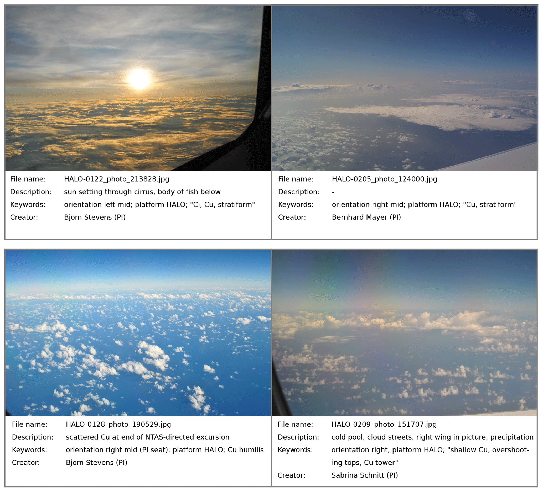
Figure 4Example photographs taken on board HALO with added metadata. The photographs are representative of the typical trade-wind organizational patterns identified by Stevens et al. (2020): Fish; Flowers; Sugar; and, in a less typical form, Gravel (from top left to bottom right).
In this section we describe data compiled and published to document HALO's state, as well as the cloud conditions sampled by its different cloud-sensitive instruments. With the exception of the dropsondes, these data are derived from, and thus introduce, the full suite of instrumentation (Table 4) included as part of the cloud-observatory configuration of HALO. Information on how to access the actual measurements from HALO's instrumental payload, some of which are independently published, is provided in Sect. 4.
Wirth et al., 2009Mech et al., 2014Wendisch et al., 2016; Stevens et al., 2019Ewald et al., 2016Schäfer et al., 2021cKrautstrunk and Giez, 2012(George et al., 2021)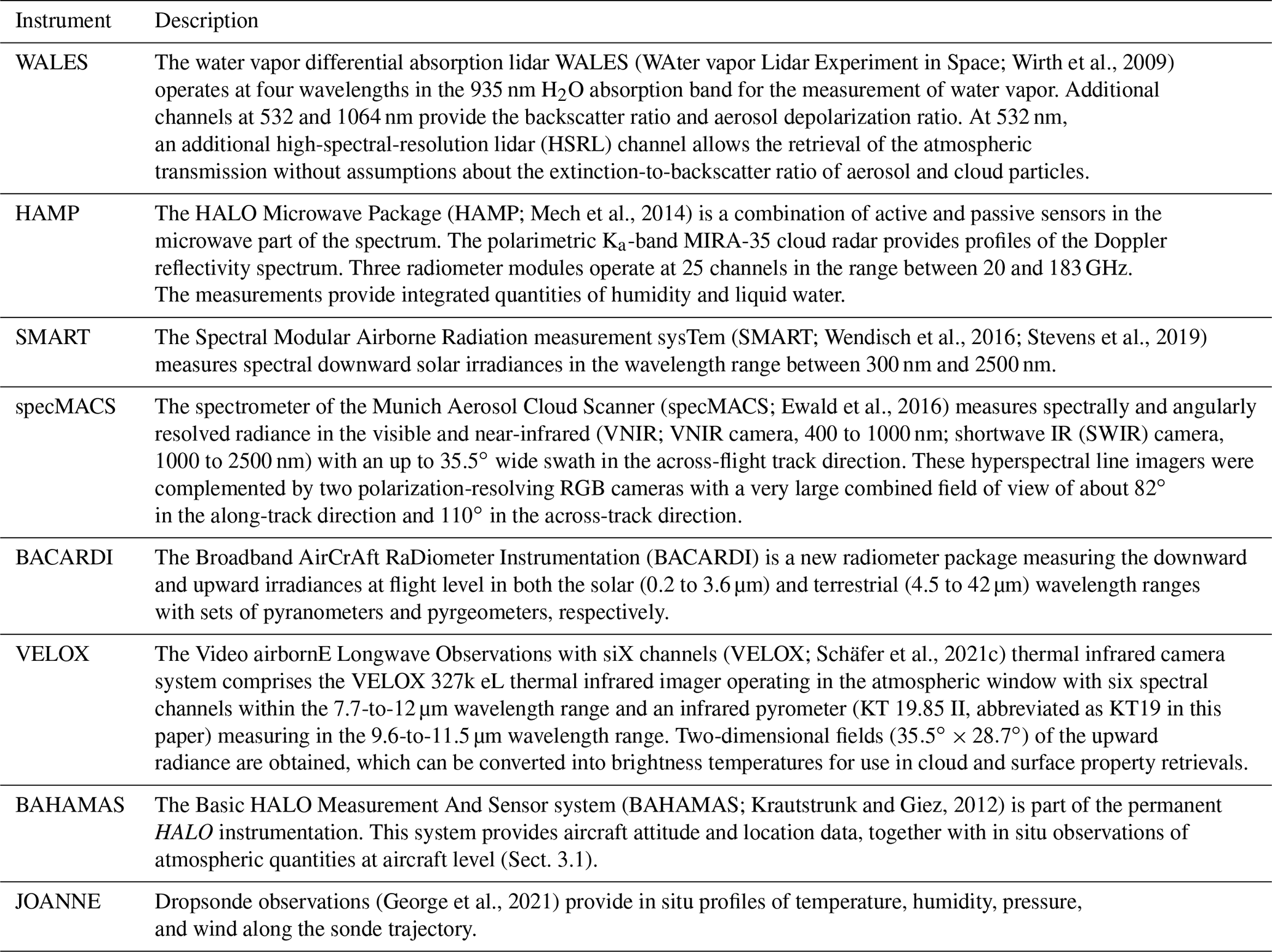
3.1 Aircraft location and attitude data
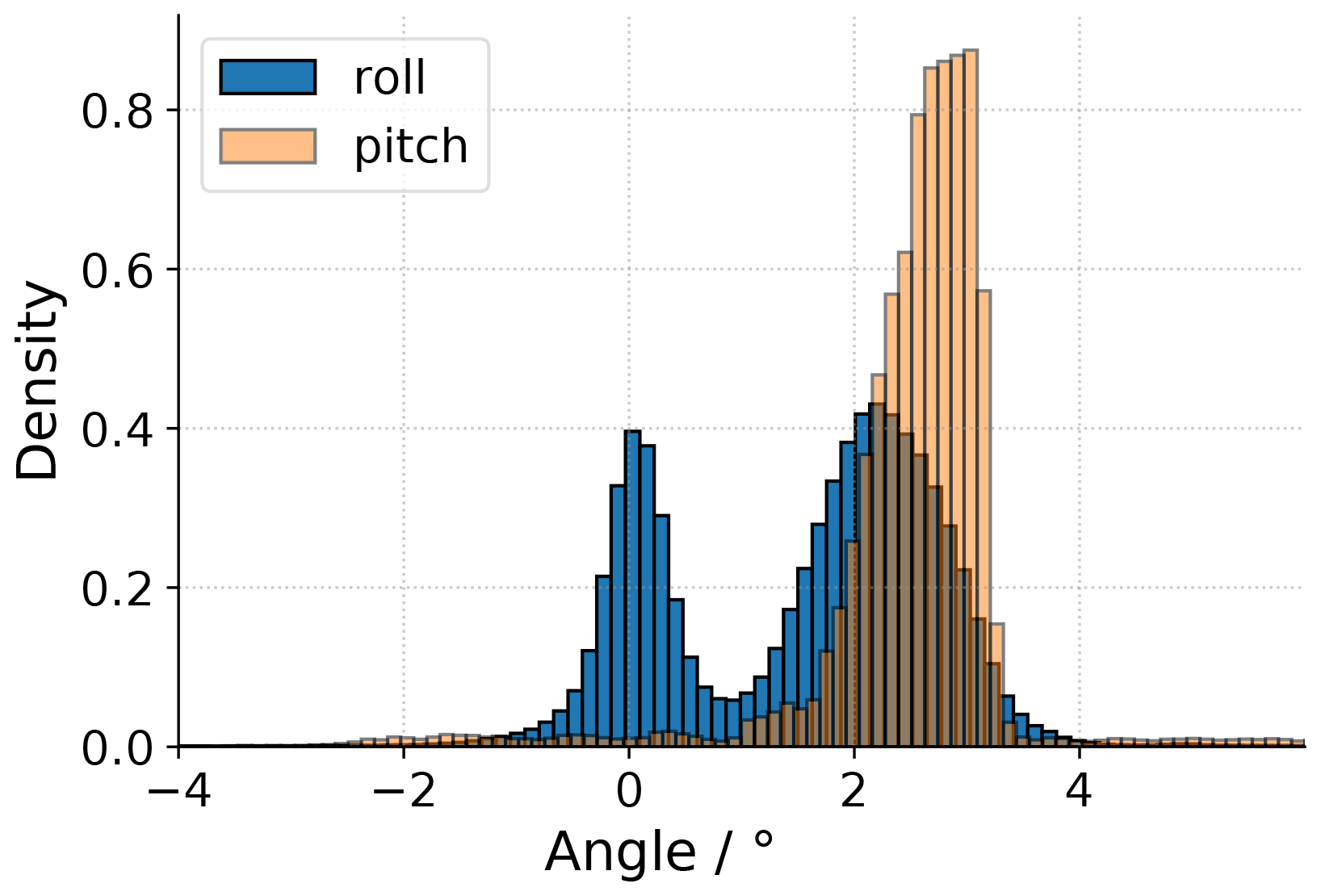
The BAsic HALO Measurement And Sensor system (BAHAMAS, Table 4) provides aircraft location and attitude data for all HALO flights, in addition to atmospheric measurements. A subset of the BAHAMAS data, consisting of the aircraft altitude, heading, latitude, longitude, roll angle, pitch angle, and true air speed with a time resolution of 10 Hz, has been created (Klingebiel, 2021). Figure 1 uses the data subset to present the tracks of all flights in the vicinity of Barbados as well as the ferry flights from and to Germany. The roll and pitch angles of all flights are shown in Fig. 5. The distribution of the roll angles (blue) shows two peaks. The one centered at 0∘ indicates straight legs, while the other centered at 2.2∘ arises from circling in a clockwise (positive roll angle) manner. The distribution of the pitch angle (orange) shows a peak near 3∘. This pitch changes systematically as fuel is burned through the flight. Although the constant roll angle on the measurements during circling is sometimes raised as a concern, this analysis shows that – for the large circles flown during EUREC4A – the non-zero pitch results in a larger deviation from the true nadir of the downward-staring instruments than does the constant roll.
3.2 Cloud masks
EUREC4A's HALO was designed to observe different properties of clouds using the richness of their interaction with electromagnetic radiation. Different instruments (Table 4), by virtue of their differing measurement principles and footprints, see clouds in different ways. Figure 6 provides a snapshot for a 5 min flight segment from flight HALO-0205 on a circle segment (HALO-0205_c2, Table 2), which represents typical cloud conditions of EUREC4A. WALES and the HAMP radar provide vertical cross sections; specMACS and VELOX provide a two-dimensional horizontal view of the clouds along the flight path, and other instruments provide a scalar time series of measurements along the flight path.
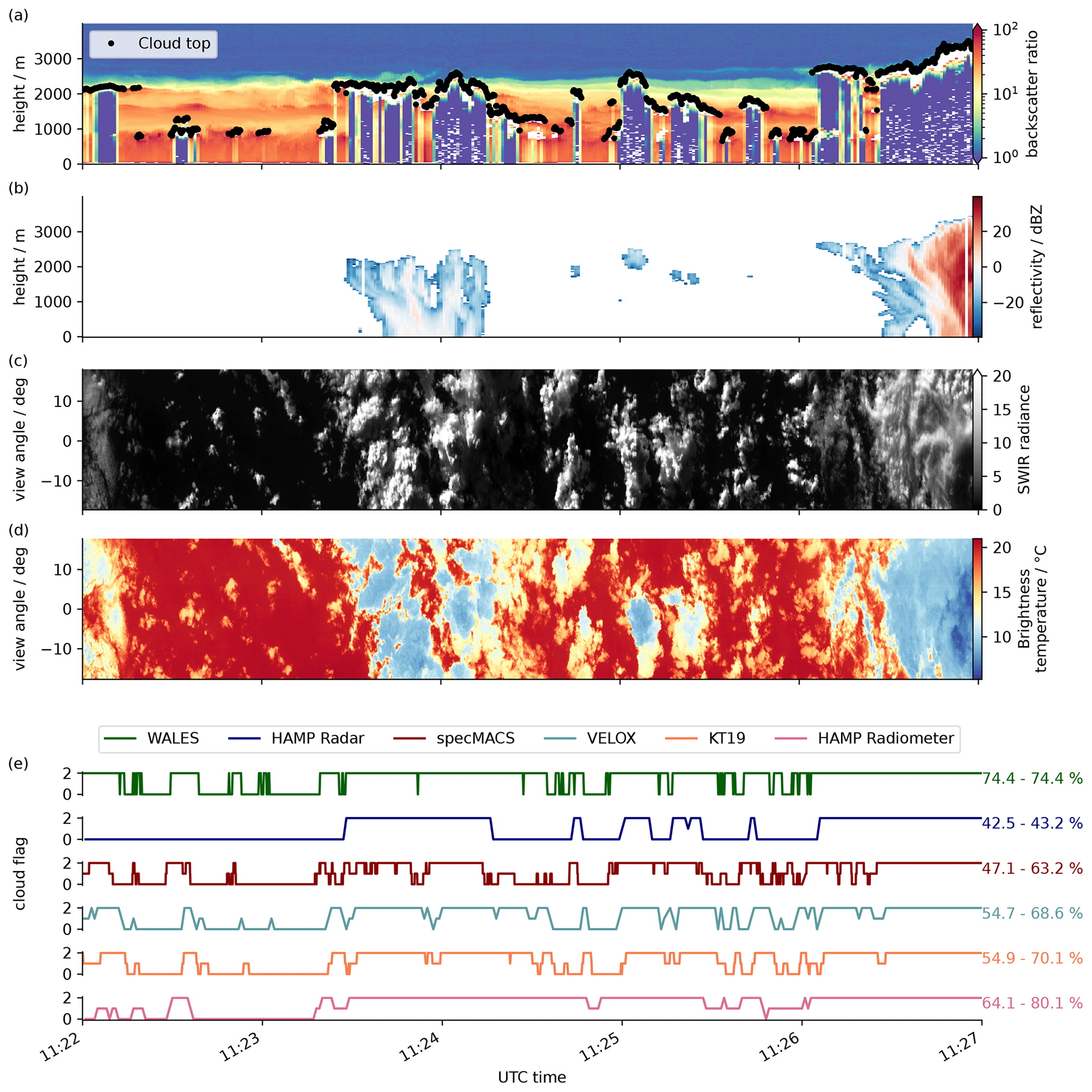
Figure 6Example scene of cloud masks from different instruments during research flight HALO-0205. Panel (a) shows the backscatter ratio at 1024 nm from WALES together with a cloud-top height estimate. Panel (b) shows the HAMP cloud radar reflectivity, panel (c) a horizontal view on the cloud field from the specMACS imager at 1.6 µm (SWIR, shortwave infrared), and panel (d) a horizontal view from the VELOX IR imager (7.7 and 12 µm). Panel (e) shows a scalar cloud mask product along the flight path from six instruments. The three cloud flag values can be used to derive a minimum or maximum cloud cover stated on the right. Minimum cloud cover includes only most likely cloudy cases; maximum cloud cover includes most likely cloudy and probably cloudy cases. For the comparison only the central 11×11 pixels (0.57∘) from VELOX and central 0.6∘ from specMACS are selected, both as close as possible to the HAMP cloud radar footprint.
To provide an overview of the cloud fields sampled by HALO, a trinary cloud mask is created for each cloud-sensitive instrument, as described in Appendix B. Access to the cloud mask data is outlined in Table 6. The value of the cloud mask denotes measurements that each instrument identifies as cloud-free (0), probably cloudy (1), or most likely cloudy (2). The introduction of the probably cloudy flag reflects the ambiguity in cloud detection faced by many instruments. Especially for the passive instruments (HAMP radiometer, specMACS, KT19, VELOX), a range of thresholds were applied to separate cloudy and cloud-free observations. Cases where the lower and upper threshold give a different decision are marked as probably cloudy. A comparison of the cloud masks (Fig. 6) shows how the cloud amount is sensitive to the manner of detecting clouds. The radar is sensitive to large drops, which form through the collision and coalescence of cloud droplets, a process that becomes active as clouds deepen and increase their condensate burden. The lidar, on the other hand, is also sensitive to optically thin clouds with a very small condensate burden. This explains the differences in the measured cloud cover by these two instruments for the 5 min segment shown in Fig. 6. The sensitivity of the passive instruments is influenced by the contrast of the cloud and surface reflection or emission. A time offset is also apparent in different cloud flags, which arises from slight differences in the instrument orientations (more forward pointing instruments detect clouds earlier than more backward pointing instruments), rather than lack of synchronicity.
The campaign average cloud-cover estimates as detected by the instruments are stated in Table 5. Most instruments define a minimum cloud cover based on the cloud flag most likely cloudy and a maximum cloud cover that additionally includes the uncertain cloud flag probably cloudy. WALES stands out as there is no probably cloudy flag in the cloud mask algorithm (Sect. B1) and the minimum and maximum cloud cover are equal. The HAMP radar seems to have very few uncertain cases.
Table 5Campaign mean cloud-cover estimates from all local research flights (22 January–15 February). Minimum cloud cover: only most likely cloudy, maximum most likely cloudy and probably cloudy cases. Note that not all instruments performed measurements at all times.
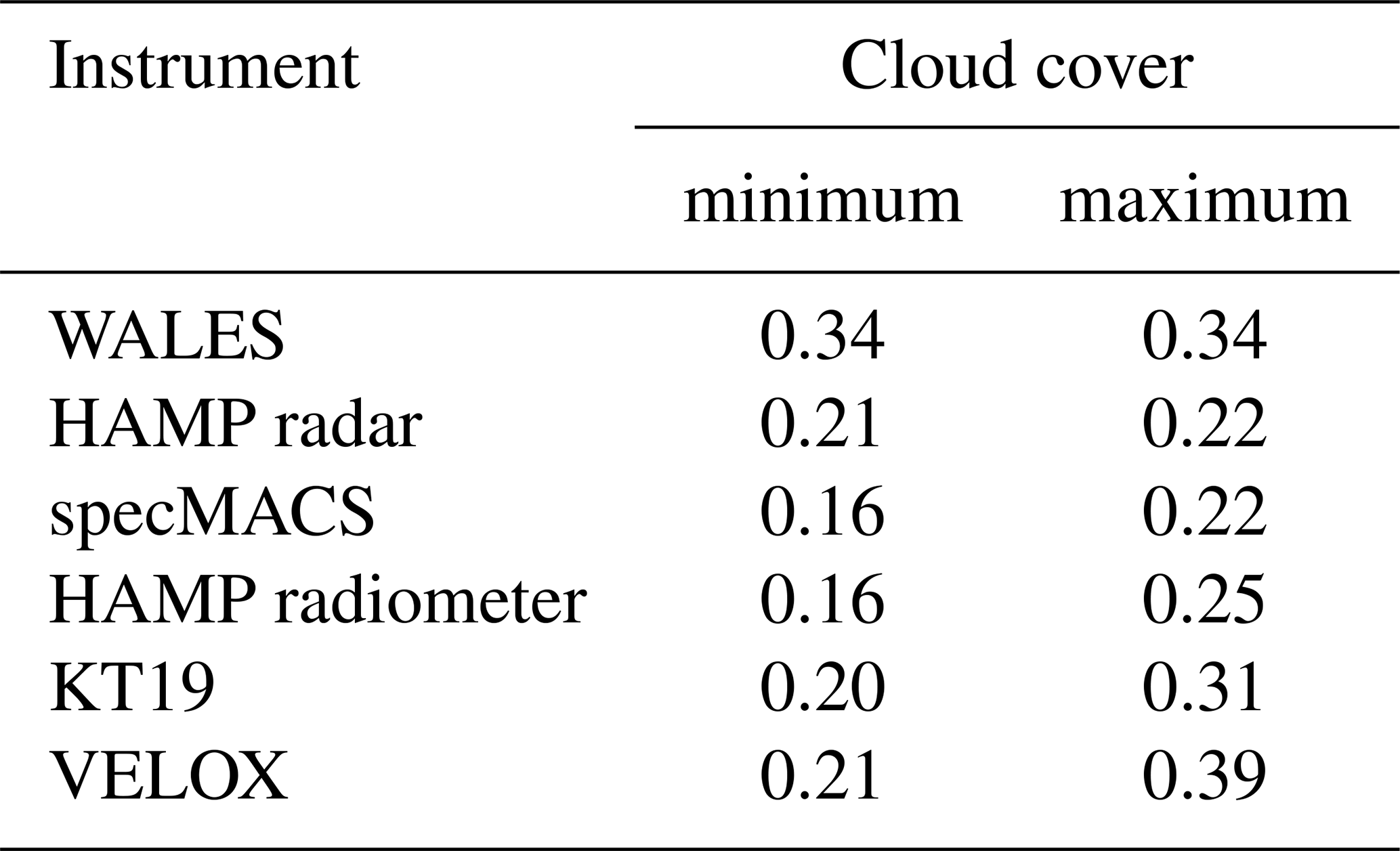
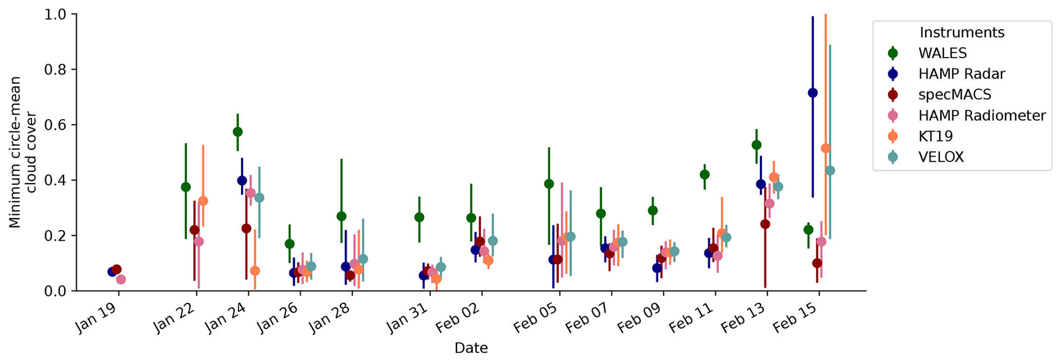
Figure 7Time series of circle-mean (minimum) cloud-cover estimates. The markers visualize the research flight average, while the lines span the range of all circle-mean cloud-cover estimates on a respective flight. Dates are given in the format MMM DD.
To provide context for the variations in cloud cover, Fig. 7 shows a time series of circle-mean (minimum) cloud-cover estimates for all research flights and from all instruments. HALO typically flew six circles per research flight (per day). In addition to the research flight mean, the whiskers span the range from the smallest to the largest circle-mean (minimum) cloud cover for each flight. In general, the individual instruments show a tendency towards higher cloud cover at the beginning as well as towards the end of the campaign. For most cases the cloud-cover estimates from passive instruments and the radar agree well. WALES systematically detects more clouds. It is more aligned with the circle-mean (maximum) cloud-cover estimates of the other instruments, as it does not include an uncertain cloud flag and is very sensitive to optically thin clouds. The flight HALO-0215 is an exception to the systematic difference between WALES and the other sensors, which is due to a deep stratocumulus layer with a strong reflection at the cloud top that blinded the lidar while the radar was still able to provide reasonable estimates.
Figure 8Cumulative fraction of circle-mean cloud-cover estimates. Depending on the instruments and some instrument downtime, the available circle counts range from 64 to 72. The bins on the x axis have a bin width of 0.2. The bars span the range defined by the minimum cloud cover based on the cloud flag most likely cloudy and by the maximum cloud cover based on cloud flags most likely cloudy and probably cloudy.
To further investigate the differences among the sensors and their cloud-masking algorithms, we display the cumulative fraction of circle-mean cloud-cover estimates in Fig. 8. In particular, the bars show the range defined by the circle-mean minimum and circle-mean maximum cloud-cover estimates for the cloud-cover ranges stated on the x axis. The differences between minimum and maximum cloud cover originate from the uncertain cases with the cloud flag probably cloudy. The first thing to note is a disagreement between the instruments for cloud cover ranges up to about 0.5 due to their different detection principles. Geometrically and optically thin clouds can have a significant impact on circle-mean estimates in low-cloud-cover situations and lead to uncertain pixels depending on the detection principle (Mieslinger et al., 2021). As WALES is able to detect optically thin clouds with few condensates, the cloud-cover estimates are generally higher, and the change in cumulative fraction is strongest between 0.2 and 0.6. The radar stands in contrast to WALES, with most circle measurements exhibiting a cloud cover below 0.2 as it cannot detect the small and optically thin clouds at the operating wavelength. The VELOX cloud mask includes a high fraction of uncertain pixels leading to a large difference (large bars) between the minimum and maximum cloud cover visible in Fig. 8 at cloud covers of up to 0.4. In the case of VELOX as well as for all other passive instruments, the cloud-cover estimates shift to higher numbers when the thresholds are reduced (from minimum to maximum cloud cover).
In general we find that only a few circles have a cloud cover higher than 0.6. At such high cloud cover the instruments agree remarkably well and, also, minimum and maximum cloud cover are almost equal, meaning that there are few or none probably cloudy measurements. Or, to put it another way, about 90 % of all circles have a cloud cover below 0.4 for most instruments except VELOX with 90 % of cloud-cover estimates below 0.6. Furthermore, about 50 % of the time cloud-cover estimates are below 0.2. The analysis of circle-mean cloud cover suggests a high abundance of low-cloud-cover situations. WALES as well as the passive instruments is capable of detecting the thinner cloud edges and small and optically thin clouds. The HAMP radar is not sensitive to these cloud parts which typically consist of small cloud droplets. The comparison illustrates the potential of the multi-instrument cloud-cover product to study cloud macro- and microphysical properties.
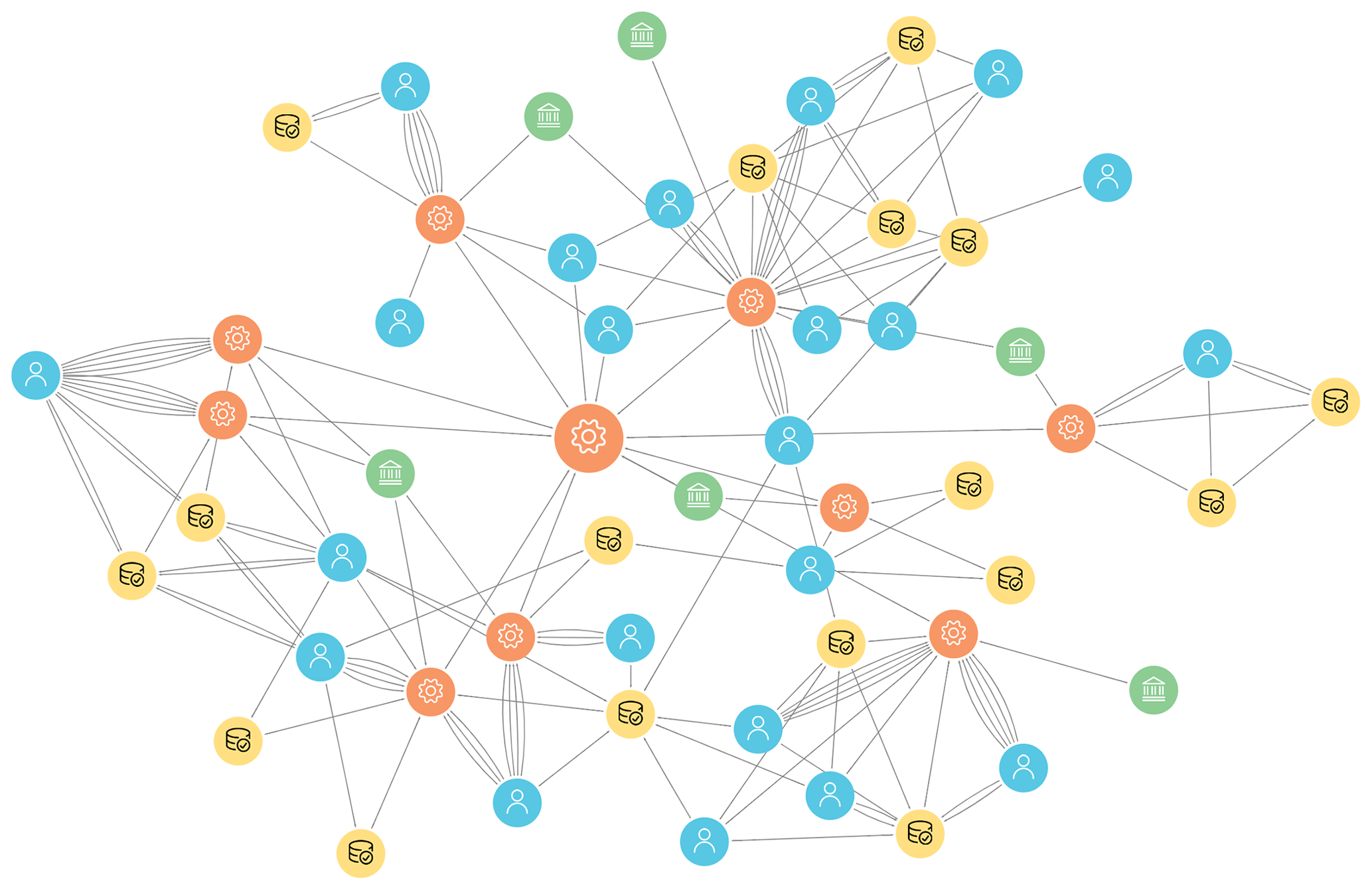
Figure 9Graphical representation of the instrument payload information that is provided in the instrument information file. The figure illustrates how HALO instrumentation is run by an interconnected community. Orange nodes are hardware; blue nodes are people; green nodes are institutions; yellow nodes are publications. Details can be found in Kölling et al. (2021) and in the How to EUREC4A book.
EUREC4A was a large field campaign, which involved hundreds of people from dozens of institutions spread over a score of countries across three continents. Measurements were collected from more sensors than there were people involved in the campaign. The task of quality controlling and curating the resultant data is immense and time-consuming. Making the data visible and usable by a broader community is even more daunting, all the more so for those same qualities that made EUREC4A's execution so successful – namely the multiplicity of people, institutions, and countries involved.
EUREC4A's HALO is a microcosm encapsulating many of the challenges faced by EUREC4A as a whole. HALO deployed instruments developed and operated by different groups, funded by different agencies, and designed to collect very different types of data. Figure 9 graphically illustrates many of these relationships. Synchronizing the processing, release, and even archiving of these data is neither practical nor desirable. Instead, to make HALO data visible and more readily usable, as new data products are also published and released, a few of the present authors created an online book. Initially the book collected and distributed use cases as a form of “how to” that others could follow. This approach to data dissemination caught on within the EUREC4A community, and investigators from other platforms added their own use cases. This led to the development of How to EUREC4A, an online and interactive Jupyter1 book. How to EUREC4A is now hosted on the EUREC4A domain2 and serves as the recommended entry point for those interested in accessing and using HALO data.
The chapters of How to EUREC4A are built from a combination of code and explanatory markdown files. The use cases range from simple examples that show how to work with HALO flight segments to simple quick looks at data from an individual instrument and to more elaborate analyses that combine measurements from different instruments. For example, the comparison of cloud cover shown in Fig. 6 is one of the use cases documented in the book. Code examples are written in Python, but the methods employed are readily transferred to other languages – even by those unfamiliar with Python. All example scripts can be run interactively in the browser via a binder integration such that no local setup and memory resources are necessary. The code examples can also be downloaded and run locally with the respective requirements for the Python environment installed. How to EUREC4A thus provides a common starting point for those interested in working with EUREC4A's HALO data and at the same time serves as a tutorial to help inexperienced users begin using the data.
How to EUREC4A is a living document. It continues to mature through the addition of chapters on new instrument platforms, through the addition of new or corrections of old analyses, and through the ingestion of new data or data releases and their provenance. For this latter purpose and to help disassociate the indexing of data from their archiving, How to EUREC4A accesses EUREC4A data through an intake catalog3, which is continuously updated to contain links to the most recent versions of the publicly available EUREC4A data. To provide users with a more narrative description of the available HALO data, How to EUREC4A also contains a section that links the HALO scientific payload with its institutional owners, contact information to its data providers, citations to reference material, and links to data. For users concerned about the volatility of an online book, a snapshot of this information, valid at the time of submission, has been compiled into a machine-readable YAML (YAML Ain't Markup Language) file (Kölling et al., 2021); it includes the information shown graphically in Fig. 9 and is included as an immutable asset with this paper.
Code and data are freely available at the locations specified in Table 6.
Prange et al. (2021)Schulz et al. (2021)Konow et al. (2021)Kölling et al. (2021)Klingebiel (2021)Jacob (2021a)Jacob (2021b)Pörtge et al. (2021)Schäfer et al. (2021a)Schäfer et al. (2021b)Wirth (2021)EUREC4A community (2021)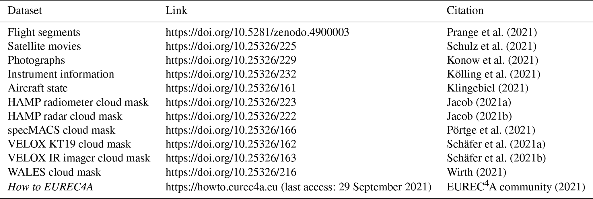
We describe the operation of the German research aircraft HALO during the EUREC4A experiment and its associated data. HALO flew 15 scientific missions during EUREC4A. These are described not only by the scientific measurements made from instruments aboard the aircraft but also through the provision of auxiliary data: timestamp intervals that segment the flight paths, selected and curated photographs from each flight, movies showing the evolving satellite presentation and flight tracks for each flight, subset aircraft state data, and cloud masks from instruments sensitive to the presence of clouds.
In addition, metadata are provided describing deployed instruments, their particular configuration, the contact information of those responsible for each instrument, and the instruments' data, and (when available) a URL to the data themselves is included, along with the aforementioned auxiliary data, through a machine-readable text (YAML) file. For convenience, Table 6 provides links to all of the data assets published with this paper. Not all datasets from the instruments that were on board HALO are assets to this paper. Most of the datasets are published separately (e.g., the dropsonde dataset JOANNE by George et al., 2021). We only describe a subset of all observed data that were taken on HALO during EUREC4A. In addition, How to EUREC4A provides a much more flexible and comprehensive, but for now volatile, description of EUREC4A's HALO's data. This book, first developed for HALO, is (as the name suggests) being extended to other instrument platforms deployed during EUREC4A. It is also being adopted by planned HALO campaigns. We hope that it will contribute to a new foundation for the treatment and dissemination of Earth system science data.
Several datasets recorded with HALO during EUREC4A continue and extend datasets that were published in earlier publications like Konow et al. (2019). These extensions, which are published alongside this paper, are described in this appendix. Detailed previous data publications are referenced for the main processing steps, and novelties or differences in the context of EUREC4A are pointed out.
A1 HAMP microwave radiometer brightness temperatures
HAMP microwave radiometer brightness temperatures observed during EUREC4A extend the dataset of previous campaigns such as NARVAL and NARVAL2, which are published by Konow et al. (2019). Compared to previous campaigns a technical update of the radiometers and their data acquisition system resulted in a reduction in the number of frequency channels from 26 to 25; i.e., the 183.3±12.5 GHz was omitted.
The quality of the original brightness temperature measurements was evaluated by comparing the measurements with synthetic ones simulated from dropsonde profiles provided in the JOANNE dataset considering the suggested humidity correction (George et al., 2021). Systematic differences which can arise from insufficient pre-flight calibration are corrected using a linear relation between recorded and synthetic brightness temperatures, which is estimated for each flight and radiometer channel. The high number of dropsondes released during each EUREC4A flight allowed the implementation of a linear correction as an update from the previous processing (Konow et al., 2019), which used a simple offset.
The radiometer data were recorded on three independent data acquisition computers. The clocks of all systems were configured such that they occasionally synchronize with the central HALO BAHAMAS system clock. However, when inspecting the time series of different recording computers, clear time offsets on the order of seconds can be identified. To correct for these time offsets, the brightness temperature time series were carefully inspected and time series of the different modules were compared with each other, the WALES data, and the radar. Doing so, we could identify offsets of between −7 and +2 s, with the exception of one module's clock running 141 s behind during the flight HALO-0119, which were subsequently corrected.
In addition, we undertook a manual inspection of the brightness temperature time series for non-atmospheric signals. This means that signals coming for example from thermal receiver instabilities and emission signals observed over transient objects like ships, which have a much higher microwave emissivity than the ocean, are discarded. The brightness temperature and time offsets are corrected. Due to the new data acquisition system, data with a high temporal resolution of a 4 Hz sampling rate are available on request in addition to the quality-controlled and published dataset.
A2 HAMP microwave radiometer retrievals
The retrieval methods developed by Jacob et al. (2019) are applied to the EUREC4A observations, and the retrieved time series of the integrated water vapor, liquid water path, and rainwater path are published in Jacob (2021c). For this dataset, we updated the training database for the artificial neural network retrieval using ICON model simulations for the EUREC4A period.
A3 HAMP cloud radar calibration
The absolute calibration of radar reflectivity measured by the HAMP cloud radar followed Ewald et al. (2019). This technique uses the well-defined ocean surface backscatter as external calibration reference. For that purpose, the angular ocean surface backscatter was sampled several times using dedicated flight maneuvers (as described in the flight segmentation data). In total, six maneuvers with a constant roll angle of 10∘ and alternating roll maneuvers of ±20∘, identified as the segments “radar calibration tilted” and “radar calibration wiggle”, respectively (Sect. 2.2), were performed during EUREC4A.
Table A1Absolute calibration offsets Δσ0 found in comparison with the ocean surface backscatter σ0 for the HAMP cloud radar during EUREC4A. Furthermore, the horizontal wind speed udrop measured by dropsondes is compared with the horizontal wind speed ufit retrieved from the angular pattern of σ0.

Based on measured signal-to-noise ratios, the normalized radar cross section σ0 was calculated using the system parameters listed in Ewald et al. (2019). Due to a receiver update and a frequency change from 35.5 to 35.17 GHz, the antenna gain (Ga=49.0 dBi) and the receiver noise figure (NF=8.4 dB) had to be redetermined in laboratory measurements. After correcting measured for gaseous attenuation, they could be compared to modeled σ0 using horizontal wind speed data from collocated dropsonde soundings analogously to in Ewald et al. (2019). In Table A1 the absolute calibration offsets found, , are summarized for each successful calibration pattern. In addition, Table A1 compares the horizontal wind speed udrop measured by the dropsondes with the horizontal wind speed ufit retrieved from the angular pattern of . In summary, an absolute calibration offset of +1.7 dB was found for the EUREC4A deployment of the HAMP cloud radar and subsequently subtracted from the radar reflectivity for the unified dataset.
In the following the methods used to construct cloud masks for each instrument are detailed.
B1 WALES
For the WALES cloud mask, lidar raw data at a temporal resolution of 5 Hz were used, which corresponds to 40 m horizontal spacing. The vertical resolution of the backscatter data is 7.5 m. The cloud flag is inferred from a step of the lidar backscatter ratio at 532 nm to values bigger than 10 while searching from the aircraft downward. The limit value of 10 is higher than what is expected from dry aerosol at this time of the season and thus indicates that considerable water uptake has occurred. To further facilitate the discrimination of optically thin clouds and opaque ones, the atmospheric optical depth between the cloud top and the sub-cloud layer is included in the dataset. Values above 2 to 3, depending on the background light situation, are only rough estimates but indicate the presence of an optically thick, opaque cloud. The details of this method, which is based on the HSRL channel, can be found in Esselborn et al. (2008). The data also include the altitude of the cloud top as the height above the EGM96 geoid with a precision of about 10 m and an accuracy of about the same magnitude. Also included is an estimation of the altitude of the top of the boundary layer above sea level. This is inferred from the maximum correlation of the lidar backscatter ratio profile at 532 nm with a step function. This quantity is experimental and should be interpreted with care, especially in the presence of residual layers or strong horizontal wind shear, which may cause multi-layer structures. In the case of a cloud, no boundary layer top is given. To enable precise comparisons with other instruments, the WALES cloud-top data also include the position of the target cloud in addition to the coordinates of the aircraft. These two locations may differ by several kilometers depending on the roll angle. This cloud mask dataset is published (Wirth, 2021) and is available for download under https://doi.org/10.25326/216.
B2 HAMP (cloud radar)
The HAMP radar cloud mask uses radar reflectivities measured by the HAMP cloud radar and calibrated as described in Sect. A3. The data are provided at a 1 Hz time interval and with a 30 m vertical resolution. Reflectivity data are first filtered for clutter. Any signal above the noise level at 200 m above sea level or higher is considered a possible cloud. Signals originating from an object of at least 4 contiguous pixels are classified as most likely a cloud; otherwise they are classified as probably a cloud signal. The cloud mask is published by Jacob (2021b) and can be downloaded from the database (https://doi.org/10.25326/222).
B3 specMACS
The data of the shortwave infrared line camera of specMACS at a temporal resolution of 30 Hz are used to provide a cloud mask. The cloud mask is based on two criteria: the brightness of the observed pixels and the strength of absorption due to water vapor. For evaluating a scene, two reference spectra in the range from 1015 to 1300 nm (one with and the other without molecular absorption – abbreviated as Labs,λ and Lno abs,λ) are calculated. The simulated transmittance Tref,λ is then given by . These reference spectra are fitted to the measured radiances (Lmeas,λ) using the following equation:
The fit parameter a scales with the brightness of the measurements, and the parameter x is a measure of absorption. Two different thresholds are applied to the brightness fit parameter to discriminate between most likely cloudy (if the brightness of a pixel is higher than the upper threshold), probably cloudy (if the brightness is between both thresholds), and cloud-free pixels (if the brightness is smaller than the lower threshold). This brightness criterion is not sufficient for ocean areas influenced by sun glint, which can be misclassified as cloudy due to the bright glint. To address this case, sun-glint situations are first identified by theoretical considerations depending on solar illumination and viewing geometry. Because the near-surface abundance of water vapor results in a much larger water vapor path length in cloud-free versus cloudy scenes, the latter can be distinguished from the former by the water vapor absorption. The absorption is derived from the measurements using the second fit parameter x. The threshold for this fit parameter is initially derived by visual inspection of a reference scene. Afterwards it is adapted dynamically depending on the viewing zenith angle of the camera, the solar zenith angle, and the column-integrated water vapor density of ECMWF ERA5 reanalysis data. If sun glint is present, this method is applied to all pixels classified as either probably or most likely cloudy. Pixels with a strong vapor absorption signal are set to cloud-free. The cloud mask dataset has been published (Pörtge et al., 2021) and is accessible for download (https://doi.org/10.25326/166).
B4 VELOX (IR imager)
A two-dimensional cloud mask from VELOX has been derived with a similar method using brightness temperature measurements from the broadband channel of the instrument at a temporal resolution of 1 Hz. In this case, four thresholds (0.5, 1.0, 1.5, and 2.0 K) are used to determine a cloud mask flag for each spatial pixel in the field. As with the KT19 cloud mask, if one threshold is exceeded, the pixel is flagged as probably cloudy, whereas all thresholds must be exceeded for the pixel to receive a most likely cloudy flag. Furthermore, a maximum and minimum possible cloud cover within the field of view has been calculated for each time step based on the number of probably cloudy and most likely cloudy pixels, respectively. This cloud mask dataset has also been published (Schäfer et al., 2021b) and is available for download (https://doi.org/10.25326/163).
B5 VELOX (KT19)
The cloud mask from the KT19 is derived by comparing the measured brightness temperature to simulated measurements in cloud-free conditions. Using three thresholds (0.7, 1.0, and 2.0 K) based on the difference between the measurements and simulations, a measurement is flagged as cloud-free when no threshold is reached, probably cloudy when one threshold is reached, or most likely cloudy when all three thresholds are reached. The cloud mask from the KT19 has been published (Schäfer et al., 2021a) and can be found in the database (https://doi.org/10.25326/162).
B6 HAMP (microwave radiometer)
The HAMP microwave radiometer cloud mask is based on thresholding liquid water path (LWP) retrievals. The LWP retrieval is based on the warm microwave emission signal by the clouds over the radiatively cold ocean surface as described by Jacob et al. (2019). Differences with respect to EUREC4A observations compared to Jacob et al. (2019) are explained in Sect. A2. The LWP observations have a 1 s temporal resolution and are representative of a footprint of about 1 km. A scene is considered probably and most likely cloudy if the LWP exceeds 20 g m−2 or 30 g m−2, respectively. These thresholds correspond to (about) 2 to 3 times, respectively, the clear-sky retrieval uncertainty. The clear-sky LWP offset correction (Jacob et al., 2019), which considers the WALES cloud mask and would allow for even lower thresholds, is not utilized here in order to provide a cloud mask that is independent of the other cloud mask products. The cloud mask is published by Jacob (2021a) and can be downloaded from the database (https://doi.org/10.25326/223).
The supplement related to this article is available online at: https://doi.org/10.5194/essd-13-5545-2021-supplement.
FA, SB, GG, SG, MJ, BM, MM, SS, BS, JV, RV, and MWe acted as principal investigators on one or more research flights. WALES operation and data quality control were performed by SG, MG, and MWi. The SMART, VELOX, and BACARDI team, who took care of instrument design, operation, and/or data quality control, is made up of AE, AEL, MS, MWe, KW, and MZ. FA, SC, FE, GG, MH, LH, MJ, FJ, MK, HK, MM, JR, HS, and AW made up the HAMP team, with different responsibilities for instrument design and improvement, instrument calibration, instrument operation, data quality control, and product generation. LF, TK, BM, VP, and TZ operated the specMACS instrument and ensured data quality control and product generation. AG and MZ operated the BAHAMAS system and took care of data quality control. FE updated the HAMP radar calibration for EUREC4A. MJ and AW derived the HAMP radiometer calibration data. VP coordinated the joint cloud mask product. MJ, FG, VP, MS, and MWi derived the cloud mask products for their instruments. MP derived the original flight segmentation. Flight segments were manually identified by GG, LH, TK, HK, TL, TM, and MP. HS created dataset satellite images and movies. RV and HK organized photo collection and publication. MK created and published the BAHAMAS data subset. TM, JR, and TK created the How to EUREC4A book. SB and BS devised and coordinated the EUREC4A campaign. FA led the participation of the German Research Foundation (DFG) partners. HK and BS devised and wrote the manuscript with text input from FE, GG, MJ, MK, TK, AEL, TM, VP, JR, MS, HS, and MWi. All co-authors contributed with their ideas and comments to the development of the manuscript.
The contact author has declared that neither they nor their co-authors have any competing interests.
Publisher’s note: Copernicus Publications remains neutral with regard to jurisdictional claims in published maps and institutional affiliations.
This article is part of the special issue “Elucidating the role of clouds–circulation coupling in climate: datasets from the 2020 (EUREC4A) field campaign”. It is not associated with a conference.
We would like to thank Vincent Douet from AERIS and the AERIS team for their support in publishing the various datasets associated with this paper. The HALO flights would not have been possible without the support and work of the flight operations team. Thanks go to the entire team for their support in the planning and execution of these flights.
This work was supported by the Max Planck Society and DFG HALO SPP 1294. Sandrine Bony, Jessica Vial, and Raphaela Vogel have received funding from the European Research Council (ERC) under the European Union's Horizon 2020 research and innovation program (grant agreement no. 694768).
This paper was edited by David Carlson and reviewed by three anonymous referees.
Bony, S., Stevens, B., Ament, F., Bigorre, S., Chazette, P., Crewell, S., Delanoë, J., Emanuel, K., Farrell, D., Flamant, C., Gross, S., Hirsch, L., Karstensen, J., Mayer, B., Nuijens, L., Ruppert, J. H., Sandu, I., Siebesma, P., Speich, S., Szczap, F., Totems, J., Vogel, R., Wendisch, M., and Wirth, M.: EUREC4A: A Field Campaign to Elucidate the Couplings Between Clouds, Convection and Circulation, Surv. Geophys., 38, 1529–1568, https://doi.org/10.1007/s10712-017-9428-0, 2017. a, b
Esselborn, M., Wirth, M., Fix, A., Tesche, M., and Ehret, G.: Airborne high spectral resolution lidar for measuring aerosol extinction and backscatter coefficients, Appl. Optics, 47, 346–358, https://doi.org/10.1364/AO.47.000346, 2008. a
EUREC4A community: EUREC4A2021, available at: https://howto.eurec4a.eu, last access: 29 September 2021. a
Ewald, F., Kölling, T., Baumgartner, A., Zinner, T., and Mayer, B.: Design and characterization of specMACS, a multipurpose hyperspectral cloud and sky imager, Atmos. Meas. Tech., 9, 2015–2042, https://doi.org/10.5194/amt-9-2015-2016, 2016. a, b
Ewald, F., Groß, S., Hagen, M., Hirsch, L., Delanoë, J., and Bauer-Pfundstein, M.: Calibration of a 35 GHz airborne cloud radar: lessons learned and intercomparisons with 94 GHz cloud radars, Atmos. Meas. Tech., 12, 1815–1839, https://doi.org/10.5194/amt-12-1815-2019, 2019. a, b, c
Fildier, B., Touzé-Peiffer, L., and Schulz, H.: bfildier/EUREC4A_movies: v1.0.0, Zenodo [code], https://doi.org/10.5281/zenodo.4777954, 2021. a
George, G., Stevens, B., Bony, S., Pincus, R., Fairall, C., Schulz, H., Kölling, T., Kalen, Q. T., Klingebiel, M., Konow, H., Lundry, A., Prange, M., and Radtke, J.: JOANNE: Joint dropsonde Observations of the Atmosphere in tropical North atlaNtic meso-scale Environments, Earth Syst. Sci. Data, 13, 5253–5272, https://doi.org/10.5194/essd-13-5253-2021, 2021. a, b, c, d
GOES-R Calibration Working Group and GOES-R Series Program: NOAA GOES-R Series Advanced Baseline Imager (ABI) Level 1b Radiances, NOAA National Centers for Environmental Information [data set], https://doi.org/10.7289/V5BV7DSR, 2017. a
Jacob, M.: Cloud mask derived from airborne HAMP Microwave Radiometer measurements during the EUREC4A field campaign, Aeris [data set], https://doi.org/10.25326/223, 2021a. a, b
Jacob, M.: Cloud mask derived from airborne HAMP Cloud Radar measurements during the EUREC4A field campaign, Aeris [data set], https://doi.org/10.25326/222, 2021b. a, b
Jacob, M.: Liquid water path and integrated water vapor derived from airborne HAMP on HALO during the EUREC4A Field Campaign, Aeris [data set], https://doi.org/10.25326/247, 2021c. a
Jacob, M., Ament, F., Gutleben, M., Konow, H., Mech, M., Wirth, M., and Crewell, S.: Investigating the liquid water path over the tropical Atlantic with synergistic airborne measurements, Atmos. Meas. Tech., 12, 3237–3254, https://doi.org/10.5194/amt-12-3237-2019, 2019. a, b, c, d
Klepp, C., Ament, F., Bakan, S., Hirsch, L., and Stevens, B.: NARVAL Campaign Report, Tech. rep., Max-Planck-Institut für Meteorologie, available at: https://mpimet.mpg.de/fileadmin/publikationen/Reports/WEB_BzE_164_last.pdf (last access: 29 September 2021), 2014. a
Klingebiel, M.: Position and altitude data from the DLR BAHAMAS instrument during the EUREC4A Field Campaign, Aeris [data set], https://doi.org/10.25326/161, 2021. a, b
Kölling, T., Ament, F., Bony, S., Ehrlich, A., Ewald, F., George, G., Giez, A., Hirsch, L., Jacob, M., Konow, H., Mayer, B., Pörtge, V., Schäfer, M., Stevens, B., Wendisch, M., Wirth, M., Wolf, K., and Zinner, T.: Instruments on HALO during EUREC4A, references and contact points, Aeris [data set], https://doi.org/10.25326/232, 2021. a, b, c
Konow, H., Jacob, M., Ament, F., Crewell, S., Ewald, F., Hagen, M., Hirsch, L., Jansen, F., Mech, M., and Stevens, B.: A unified data set of airborne cloud remote sensing using the HALO Microwave Package (HAMP), Earth Syst. Sci. Data, 11, 921–934, https://doi.org/10.5194/essd-11-921-2019, 2019. a, b, c
Konow, H., Ament, F., Bony, S., Forster, L., George, G., Groß, S., Jacob, M., Kölling, T., Mayer, B., Mech, M., Schnitt, S., Stevens, B., Vial, J., Vogel, R., and Wendisch, M.: Photographs taken from the HALO aircraft during the EUREC4A field campaign, Aeris [data set], https://doi.org/10.25326/229, 2021. a, b
Krautstrunk, M. and Giez, A.: The Transition From FALCON to HALO Era Airborne Atmospheric Research, Springer Berlin Heidelberg, Berlin, Heidelberg, 609–624, https://doi.org/10.1007/978-3-642-30183-4_37, 2012. a, b, c
Mech, M., Orlandi, E., Crewell, S., Ament, F., Hirsch, L., Hagen, M., Peters, G., and Stevens, B.: HAMP – the microwave package on the High Altitude and LOng range research aircraft (HALO), Atmos. Meas. Tech., 7, 4539–4553, https://doi.org/10.5194/amt-7-4539-2014, 2014. a, b
Mieslinger, T., Stevens, B., Kölling, T., Brath, M., Wirth, M., and Buehler, S. A.: Optically thin clouds in the trades, Atmos. Chem. Phys. Discuss. [preprint], https://doi.org/10.5194/acp-2021-453, in review, 2021. a
Pörtge, V., Gödde, F., Kölling, T., Zinner, T., Forster, L., and Mayer, B.: Cloud mask and cloud fraction derived from solar reflectivity measurements of the imaging spectrometer specMACS on HALO during the EUREC4A field campaign, Aeris [data set], https://doi.org/10.25326/166, 2021. a, b
Prange, M., Ringel, M., George, G., Hirsch, L., Kölling, T., Konow, H., Lang, T., Mieslinger, T., Pincus, R., and Saffin, L.: EUREC4A: HALO flight phase separation: Beautiful Budgie, Zenodo [data set], https://doi.org/10.5281/zenodo.4900003, 2021. a, b
Satoh, M., Stevens, B., Judt, F., Khairoutdinov, M., Lin, S.-J., Putman, W. M., and Düben, P.: Global Cloud-Resolving Models, Current Climate Change Reports, 5, 172–184, https://doi.org/10.1007/s40641-019-00131-0, 2019. a
Schäfer, M., Ehrlich, A., Luebke, A., Thoböll, J., Wolf, K., and Wendisch, M.: Cloud mask derived from airborne KT19 measurements during the EUREC4A field campaign, Aeris [data set], https://doi.org/10.25326/162, 2021a. a, b
Schäfer, M., Ehrlich, A., Luebke, A., Thoböll, J., Wolf, K., and Wendisch, M.: Two-dimensional cloud mask and cloud fraction with 1 Hz temporal resolution derived from VELOX during the EUREC4A field campaign, Aeris [data set], https://doi.org/10.25326/163, 2021b. a, b
Schäfer, M., Wolf, K., Ehrlich, A., Hallbauer, C., Jäkel, E., Jansen, F., Luebke, A. E., Müller, J., Thoböll, J., Röschenthaler, T., Stevens, B., and Wendisch, M.: VELOX – A new thermal infrared imager for airborne remote sensing of cloud and surface properties, Atmos. Meas. Tech. Discuss. [preprint], https://doi.org/10.5194/amt-2021-341, in review, 2021c. a
Schulz, H., Touzé-Peiffer, L., and Fildier, B.: EUREC4A GOES-16 ABI overview movies (VIS+IR), Aeris [data set], https://doi.org/10.25326/225, 2021. a, b
Stevens, B., Farrell, D., Hirsch, L., Jansen, F., Nuijens, L., Serikov, I., Brügmann, B., Forde, M., Linné, H., Lonitz, K., and Prospero, J. M.: The Barbados Cloud Observatory: anchoring investigations of clouds and circulation on the edge of the ITCZ, B. Am. Meteorol. Soc., 97, 787–801, https://doi.org/10.1175/BAMS-D-14-00247.1, 2016. a, b
Stevens, B., Ament, F., Bony, S., Crewell, S., Ewald, F., Gross, S., Hansen, A., Hirsch, L., Jacob, M., Kölling, T., Konow, H., Mayer, B., Wendisch, M., Wirth, M., Wolf, K., Bakan, S., Bauer-Pfundstein, M., Brueck, M., Delanoë, J., Ehrlich, A., Farrell, D., Forde, M., Gödde, F., Grob, H., Hagen, M., Jäkel, E., Jansen, F., Klepp, C., Klingebiel, M., Mech, M., Peters, G., Rapp, M., Wing, A. A., and Zinner, T.: A High-Altitude Long-Range Aircraft Configured as a Cloud Observatory: The NARVAL Expeditions, B. Am. Meteorol. Soc., 100, 1061–1077, https://doi.org/10.1175/BAMS-D-18-0198.1, 2019. a, b, c
Stevens, B., Bony, S., Brogniez, H., Hentgen, L., Hohenegger, C., Kiemle, C., L'Ecuyer, T. S., Naumann, A. K., Schulz, H., Siebesma, P. A., Vial, J., Winker, D. M., and Zuidema, P.: Sugar, gravel, fish and flowers: Mesoscale cloud patterns in the trade winds, Q. J. Roy. Meteor. Soc., 146, 141–152, https://doi.org/10.1002/qj.3662, 2020. a, b
Stevens, B., Bony, S., Farrell, D., Ament, F., Blyth, A., Fairall, C., Karstensen, J., Quinn, P. K., Speich, S., Acquistapace, C., Aemisegger, F., Albright, A. L., Bellenger, H., Bodenschatz, E., Caesar, K.-A., Chewitt-Lucas, R., de Boer, G., Delanoë, J., Denby, L., Ewald, F., Fildier, B., Forde, M., George, G., Gross, S., Hagen, M., Hausold, A., Heywood, K. J., Hirsch, L., Jacob, M., Jansen, F., Kinne, S., Klocke, D., Kölling, T., Konow, H., Lothon, M., Mohr, W., Naumann, A. K., Nuijens, L., Olivier, L., Pincus, R., Pöhlker, M., Reverdin, G., Roberts, G., Schnitt, S., Schulz, H., Siebesma, A. P., Stephan, C. C., Sullivan, P., Touzé-Peiffer, L., Vial, J., Vogel, R., Zuidema, P., Alexander, N., Alves, L., Arixi, S., Asmath, H., Bagheri, G., Baier, K., Bailey, A., Baranowski, D., Baron, A., Barrau, S., Barrett, P. A., Batier, F., Behrendt, A., Bendinger, A., Beucher, F., Bigorre, S., Blades, E., Blossey, P., Bock, O., Böing, S., Bosser, P., Bourras, D., Bouruet-Aubertot, P., Bower, K., Branellec, P., Branger, H., Brennek, M., Brewer, A., Brilouet, P.-E., Brügmann, B., Buehler, S. A., Burke, E., Burton, R., Calmer, R., Canonici, J.-C., Carton, X., Cato Jr., G., Charles, J. A., Chazette, P., Chen, Y., Chilinski, M. T., Choularton, T., Chuang, P., Clarke, S., Coe, H., Cornet, C., Coutris, P., Couvreux, F., Crewell, S., Cronin, T., Cui, Z., Cuypers, Y., Daley, A., Damerell, G. M., Dauhut, T., Deneke, H., Desbios, J.-P., Dörner, S., Donner, S., Douet, V., Drushka, K., Dütsch, M., Ehrlich, A., Emanuel, K., Emmanouilidis, A., Etienne, J.-C., Etienne-Leblanc, S., Faure, G., Feingold, G., Ferrero, L., Fix, A., Flamant, C., Flatau, P. J., Foltz, G. R., Forster, L., Furtuna, I., Gadian, A., Galewsky, J., Gallagher, M., Gallimore, P., Gaston, C., Gentemann, C., Geyskens, N., Giez, A., Gollop, J., Gouirand, I., Gourbeyre, C., de Graaf, D., de Groot, G. E., Grosz, R., Güttler, J., Gutleben, M., Hall, K., Harris, G., Helfer, K. C., Henze, D., Herbert, C., Holanda, B., Ibanez-Landeta, A., Intrieri, J., Iyer, S., Julien, F., Kalesse, H., Kazil, J., Kellman, A., Kidane, A. T., Kirchner, U., Klingebiel, M., Körner, M., Kremper, L. A., Kretzschmar, J., Krüger, O., Kumala, W., Kurz, A., L'Hégaret, P., Labaste, M., Lachlan-Cope, T., Laing, A., Landschützer, P., Lang, T., Lange, D., Lange, I., Laplace, C., Lavik, G., Laxenaire, R., Le Bihan, C., Leandro, M., Lefevre, N., Lena, M., Lenschow, D., Li, Q., Lloyd, G., Los, S., Losi, N., Lovell, O., Luneau, C., Makuch, P., Malinowski, S., Manta, G., Marinou, E., Marsden, N., Masson, S., Maury, N., Mayer, B., Mayers-Als, M., Mazel, C., McGeary, W., McWilliams, J. C., Mech, M., Mehlmann, M., Meroni, A. N., Mieslinger, T., Minikin, A., Minnett, P., Möller, G., Morfa Avalos, Y., Muller, C., Musat, I., Napoli, A., Neuberger, A., Noisel, C., Noone, D., Nordsiek, F., Nowak, J. L., Oswald, L., Parker, D. J., Peck, C., Person, R., Philippi, M., Plueddemann, A., Pöhlker, C., Pörtge, V., Pöschl, U., Pologne, L., Posyniak, M., Prange, M., Quiñones Meléndez, E., Radtke, J., Ramage, K., Reimann, J., Renault, L., Reus, K., Reyes, A., Ribbe, J., Ringel, M., Ritschel, M., Rocha, C. B., Rochetin, N., Röttenbacher, J., Rollo, C., Royer, H., Sadoulet, P., Saffin, L., Sandiford, S., Sandu, I., Schäfer, M., Schemann, V., Schirmacher, I., Schlenczek, O., Schmidt, J., Schröder, M., Schwarzenboeck, A., Sealy, A., Senff, C. J., Serikov, I., Shohan, S., Siddle, E., Smirnov, A., Späth, F., Spooner, B., Stolla, M. K., Szkółka, W., de Szoeke, S. P., Tarot, S., Tetoni, E., Thompson, E., Thomson, J., Tomassini, L., Totems, J., Ubele, A. A., Villiger, L., von Arx, J., Wagner, T., Walther, A., Webber, B., Wendisch, M., Whitehall, S., Wiltshire, A., Wing, A. A., Wirth, M., Wiskandt, J., Wolf, K., Worbes, L., Wright, E., Wulfmeyer, V., Young, S., Zhang, C., Zhang, D., Ziemen, F., Zinner, T., and Zöger, M.: EUREC4A, Earth Syst. Sci. Data, 13, 4067–4119, https://doi.org/10.5194/essd-13-4067-2021, 2021. a, b, c
Wendisch, M., Müller, D., Schell, D., and Heintzenberg, J.: An Airborne Spectral Albedometer with Active Horizontal Stabilization, J. Atmos. Ocean. Tech., 18, 1856–1866, https://doi.org/10.1175/1520-0426(2001)018<1856:AASAWA>2.0.CO;2, 2001. a
Wendisch, M., Pöschl, U., Andreae, M. O., Machado, L. A. T., Albrecht, R., Schlager, H., Rosenfeld, D., Martin, S. T., Abdelmonem, A., Afchine, A., Araùjo, A. C., Artaxo, P., Aufmhoff, H., Barbosa, H. M. J., Borrmann, S., Braga, R., Buchholz, B., Cecchini, M. A., Costa, A., Curtius, J., Dollner, M., Dorf, M., Dreiling, V., Ebert, V., Ehrlich, A., Ewald, F., Fisch, G., Fix, A., Frank, F., Fütterer, D., Heckl, C., Heidelberg, F., Hüneke, T., Jäkel, E., Järvinen, E., Jurkat, T., Kanter, S., Kästner, U., Kenntner, M., Kesselmeier, J., Klimach, T., Knecht, M., Kohl, R., Kölling, T., Krämer, M., Krüger, M., Krisna, T. C., Lavric, J. V., Longo, K., Mahnke, C., Manzi, A. O., Mayer, B., Mertes, S., Minikin, A., Molleker, S., Münch, S., Nillius, B., Pfeilsticker, K., Pöhlker, C., Roiger, A., Rose, D., Rosenow, D., Sauer, D., Schnaiter, M., Schneider, J., Schulz, C., de Souza, R. A. F., Spanu, A., Stock, P., Vila, D., Voigt, C., Walser, A., Walter, D., Weigel, R., Weinzierl, B., Werner, F., Yamasoe, M. A., Ziereis, H., Zinner, T., and Zöger, M.: Acridicon-chuva campaign: Studying tropical deep convective clouds and precipitation over Amazonia using the New German research aircraft HALO, B. Am. Meteorol. Soc., 97, 1885–1908, https://doi.org/10.1175/BAMS-D-14-00255.1, 2016. a, b
Wessel, P. and Smith, W. H. F.: A global, self-consistent, hierarchical, high-resolution shoreline database, J. Geophys. Res., 101, 8741–8743, https://doi.org/10.1029/96JB00104, 1996. a, b
Wirth, M.: Cloud top height derived from airborne measurements with the WALES lidar during the EUREC4A field campaign, Aeris [data set], https://doi.org/10.25326/216, 2021. a, b
Wirth, M., Fix, A., Mahnke, P., Schwarzer, H., Schrandt, F., and Ehret, G.: The airborne multi-wavelength water vapor differential absorption lidar WALES: System design and performance, Appl. Phys. B-Lasers O., 96, 201–213, https://doi.org/10.1007/s00340-009-3365-7, 2009. a, b
Jupyter is an interactive development environment supporting several programming languages (https://jupyter.org, last access: 29 September 2021).
https://howto.eurec4a.eu (last access: 29 September 2021).
https://github.com/eurec4a/eurec4a-intake (last access: 29 September 2021).
- Abstract
- Introduction
- HALO during EUREC4A
- Instrumentation
- Accessing EUREC4A's HALO data
- Code and data availability
- Summary
- Appendix A: Dataset updates
- Appendix B: Cloud masks
- Author contributions
- Competing interests
- Disclaimer
- Special issue statement
- Acknowledgements
- Financial support
- Review statement
- References
- Supplement