the Creative Commons Attribution 4.0 License.
the Creative Commons Attribution 4.0 License.
 | 19 Nov 2021
A 1 km global cropland dataset from 10 000 BCE to 2100 CE
Bowen Cao
Xuecao Li
Min Chen
Pengyu Hao
Peng Gong
Cropland greatly impacts food security, energy supply, biodiversity, biogeochemical cycling, and climate change. Accurately and systematically understanding the effects of agricultural activities requires cropland spatial information with high resolution and a long time span. In this study, the first 1 km resolution global cropland proportion dataset for 10 000 BCE–2100 CE was produced. With the cropland map initialized in 2010 CE, we first harmonized the cropland demands extracted from the History Database of the Global Environment 3.2 (HYDE 3.2) and the Land-Use Harmonization 2 (LUH2) datasets and then spatially allocated the demands based on the combination of cropland suitability, kernel density, and other constraints. According to our maps, cropland originated from several independent centers and gradually spread to other regions, influenced by some important historical events. The spatial patterns of future cropland change differ in various scenarios due to the different socioeconomic pathways and mitigation levels. The global cropland area generally shows an increasing trend over the past years, from 0×106 km2 in 10 000 BCE to 2.8×10⁶ km2 in 1500 CE, 6.2×10⁶ km2 in 1850 CE, and 16.4×10⁶ km2 in 2010 CE. It then follows diverse trajectories under future scenarios, with the growth rate ranging from 16.4 % to 82.4 % between 2010 CE and 2100 CE. There are large area disparities among different geographical regions. The mapping result coincides well with widely used datasets at present in both distribution pattern and total amount. With improved spatial resolution, our maps can better capture the cropland distribution details and spatial heterogeneity. The spatiotemporally continuous and conceptually consistent global cropland dataset serves as a more comprehensive alternative for long-term earth system simulations and other precise analyses. The flexible and efficient harmonization and downscaling framework can be applied to specific regions or extended to other land use and cover types through the adjustable parameters and open model structure. The 1 km global cropland maps are available at https://doi.org/10.5281/zenodo.5105689 (Cao et al., 2021a).
- Article
(11087 KB) - Full-text XML
- BibTeX
- EndNote


Land use changes driven by humans have profound impacts on climate change, biogeochemical cycling, biodiversity, energy supply, and food security (Foley et al., 2005; Kalnay and Cai, 2003; Ito and Hajima, 2020; Poschlod et al., 2005). As one of the predominant land use types, agricultural land serves as the important carbon budget component and the basic elements of food production, contributing substantially to global change in both the natural environment system and the socioeconomic system (Friedlingstein et al., 2020; Godfray et al., 2010). In recent decades, significant progress has been made in agricultural monitoring, including cropland extents (Yu et al., 2013; Lu et al., 2020), cropland types (Cao et al., 2021b), crops (Zhong et al., 2014; Bargiel, 2017), and farming practices (Biradar and Xiao, 2011; Estel et al., 2015), providing basic and direct information to support specific research and management for specific years or periods. In comparison, simulating or analyzing the effect of cropland change from the beginning of farming to the end of this century can provide a comprehensive view for understanding agriculture, which is of great significance for establishing long-term environmental or economic strategies (Olofsson and Hickler, 2008; Pongratz et al., 2009; Molotoks et al., 2018; Zabel et al., 2019). However, big gaps and uncertainties remain in quantifying the long-term global change through models and other geospatial analysis methods, largely affected by the input land use and cover data (Prestele et al., 2017). Therefore, accurate global cropland change information, especially a harmonized cropland dataset at high resolution from past to future, plays a crucial role in improving the simulation accuracy and supporting the detailed analysis.
Some efforts have been made in developing historical or future cropland products. In reconstructing the spatial distribution of past cropland, the representative products at global-scale include the Sustainability and the Global Environment (SAGE) dataset ( resolution for global cropland during 1700 CE–1992 CE) (Ramankutty and Foley, 1999), the Millennium Land Cover Reconstruction (ML08) dataset ( resolution for global agricultural areas during 800 CE–1992 CE) (Pongratz et al., 2008), the Kaplan and Krumhardt (KK10) dataset ( resolution for 6050 BCE–1850 CE) (Kaplan et al., 2011), and the History Database of the Global Environment (HYDE) dataset (Klein Goldewijk, 2001; Klein Goldewijk et al., 2010, 2017). Among these datasets, the HYDE dataset is constantly updated, and the latest version (HYDE 3.2) achieves the highest spatial resolution ( resolution) and the longest time span (10 000 BCE–2017 CE) through a more comprehensive and reasonable algorithm (Klein Goldewijk et al., 2017). The global-scale datasets above usually employed a “top-to-bottom” method to downscale the historical records of cropland area according to the cropland suitability, population, and current distribution of cropland. Additionally, there are some regional or local products with higher resolution (Fuchs et al., 2013; Yang et al., 2015; Yu and Lu, 2018).
Research on simulating future land use and cover change has been booming in recent years, with cropland as one of the types. To prepare for each generation of the World Climate Research Program Coupled Model Intercomparison Project (CMIP), integrated assessment model (IAM) teams constructed a series of scenarios for future land use projections as inputs of Earth system models (ESMs) (O'Neill et al., 2016; Riahi et al., 2017). Based on these scenarios, the Land-Use Harmonization (LUH) project provided the harmonized land use datasets as a part of CMIP, including LUH ( resolution for 1500 CE–2100 CE) (Hurtt et al., 2011) corresponding to CMIP5 and LUH2 ( for 850 CE–2100 CE) (Hurtt et al., 2020) corresponding to CMIP6. More and more studies are devoted to future land use simulations at a higher resolution based on various scenarios to satisfy finer applications. On the global scale, there are several 1 km resolution datasets (Li et al., 2016, 2017; Cao et al., 2019). The resolutions of some local or regional downscaling research were even finer (Chen et al., 2018; Wang et al., 2018; Xu et al., 2015). Spatially explicit land use and cover change models, such as Cellular Automata (CA) (White et al., 1997), Future Land Use Simulation (FLUS) (Liu et al., 2017), Conversion of Land Use and its Effects (CLUE) (Veldkamp and Fresco, 1996), Agent-Based Model (ABM) (Matthews et al., 2007), and Demeter (Vernon et al., 2018), were extensively adopted in the future land use simulation studies.
Although the datasets above are widely used and contribute a lot to the related research, the existing global products are relatively scarce and have large uncertainty (Klein Goldewijk and Verburg, 2013; Prestele et al., 2016; Alexander et al., 2017). Huge differences between these datasets make them difficult to be well connected and even cause contradictions in applications (Prestele et al., 2017). With the development of related models and analytical methods, there is a growing demand for continuous datasets from past to future. So far, only the LUH project has provided the spatiotemporally continuous global land use datasets for the past and future. Nevertheless, although the resolution has been improved to 0.25∘ in the latest version, LUH2 is still too coarse to describe the details of cropland distribution and support accurate analysis (Schaldach et al., 2011; Liao et al., 2020). Underestimation and overestimation are inevitably caused when using low-resolution land use and cover datasets (Yu et al., 2014), which decrease the credibility of the related research results greatly. The low-resolution problem is also common in many other global-scale datasets mentioned above. Besides, since agriculture approximately originates in 10 000 BCE, the important initial period of cropland development is omitted in LUH2. Therefore, a harmonized dataset from past to future with higher resolution and longer time span is urgently needed.
As for the methods, in the studies above, historical reconstruction and future projection usually adopted different models which cannot be merged directly. Although they performed well in producing the datasets for specific periods and regions, most of them have limited extendibility in timescale or spatial scale. Some downscaling models are simple and cannot accurately characterize the long-term change, while some other models need high computational cost to implement at a large scale and fine resolution (Council, 2014). A model capable of reflecting the cropland change in time-space consistency and high efficiency is thus required. A flexible and efficient framework for harmonizing and downscaling the cropland distribution from past to future at large scale and high resolution should be established.
In the study, we produced a global cropland percentage map at 1 km resolution from 10 000 BCE to 2100 CE based on our proposed harmonization and downscaling framework, and we identified the cropland distribution patterns, estimated the cropland areas, and compared the mapping results with other datasets.
The framework of producing the 1 km global cropland dataset for 10 000 BCE–2100 CE included demand harmonization and spatial downscaling (Fig. 1). Details for the mapping procedure are provided in the following sections.
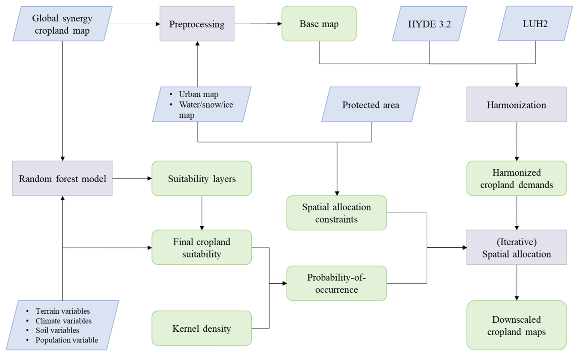
2.1 Cropland demand harmonization
Cropland demands for the past and future were estimated based on the existing products. Historical demands during 10 000 BCE–2010 CE were based on HYDE 3.2, which provides a complete historical land use reconstruction and serves as a basis of long-term global change analysis and simulation (Klein Goldewijk et al., 2017). Considering that the cropland area in HYDE 3.2 referred to the national statistics from the Food and Agriculture Organization (FAO) and subnational statistics of some larger countries (Klein Goldewijk et al., 2017), the downscaling regions in this study were divided using the provincial boundaries for several of the largest countries (countries with an area , i.e., Russia, Canada, China, America, Brazil, Australia, India, Argentina, Kazakhstan) and national boundaries for the other countries. The future demands during 2010 CE–2100 CE came from the total areas of all five crop types (including C3 annual crops, C3 perennial crops, C4 annual crops, C4 perennial crops, and C3 nitrogen-fixing crops) in the LUH2 dataset, which was consistent with the design of CMIP6 and is widely used in ESM simulations (Hurtt et al., 2020). All the eight scenarios with combinations of five Shared Socioeconomic Pathways (SSPs) and seven Representative Concentration Pathways (RCPs) (SSP1-RCP1.9, SSP1-RCP2.6, SSP2-RCP4.5, SSP3-RCP7.0, SSP4-RCP3.4, SSP4-RCP6.0, SSP5-RCP3.4OS, SSP5-RCP8.5) were projected in the study.
To drive the downscaling, an initial cropland map with the target resolution is indispensable. Here we selected the global synergy cropland map for 2010 CE produced by Lu et al. (2020) as the start point. The map was generated based on the fusion of multiple existing cropland maps and multilevel statistics of cropland area through the Self-adapting Statistics Allocation Model (SASAM). It had higher accuracy than other mainstream datasets and better consistency with the cropland statistics (Lu et al., 2020), and it used FAO's definition of cropland, i.e., “arable lands and permanent crops” (FAO, 2021), which was thus inherited into our study. In preprocessing, we first aggregated map resolution from the original 500 m to the target 1 km. Then, considering that – except cropland – urban area and water, snow, and ice (water/snow/ice) would be involved in our downscaling rules, we supplemented maps of these two land cover types from the other dataset. One of the input data for producing the global synergy cropland map, GlobeLand30 2010 (Chen et al., 2014), was selected here for its high accuracy and consistent year. To be compatible with urban and water/snow/ice distribution extracted from GlobeLand30 2010, we further processed the cropland map to ensure enough spare space is left for these types in each pixel. The non-cropland percentage in the global synergy cropland map was increased to the sum of the urban and water/snow/ice percentages in each 1 km pixel in which the former was less than the latter. The preprocessed initial cropland map was taken as the base map for the following procedures.
Due to the difference in methods and class definitions, there are obvious discrepancies in the cropland areas of HYDE 3.2, LUH2, and the base map in some regions. To avoid further errors caused by the inconsistencies, harmonizing the amount is thus necessary. We first adjusted the cropland demands in the base year (2010 CE) to keep them consistent with the cropland area of the base map. We then calculated the harmonized demands for different regions in historical and future years according to the original cropland area change rates of HYDE 3.2 and LUH2. The harmonization process can be expressed as
where is the harmonized cropland area for region r at time step t (the time-step intervals are 1000 years for 10 000 BCE–1 CE, 100 years for 1 CE–1700 CE, and 10 years for 1700 CE–2100 CE), is the cropland area of the base map for region r in 2010 CE, and and are the cropland area of HYDE 3.2 and LUH2 for region r at time step t, respectively. Namely, the demands began with the base map but followed the change trajectories of HYDE 3.2 during 10 000 BCE–2010 CE and LUH2 during 2010 CE–2100 CE. The new set of cropland demands after harmonization were prepared as inputs for the spatial downscaling.
2.2 Cropland demand downscaling
The spatial downscaling was performed based on the developed framework described below. First, the maximum area for cropland allocation in each 1 km×1 km grid cell was determined by the following rules. For the whole downscaling period (10 000 BCE–2100 CE), water, snow, and ice areas were assumed constant over time and thus could not be occupied by cropland. For the future period (2010 CE–2100 CE), cropland would not expand to the urban area due to urbanization usually being regarded as the most irreversible anthropic activity (Grimm et al., 2008; Wu, 2014), and cropland located within the protected area (defined by World Database on Protected Areas (WDPA); UNEP-WCMC and IUCN, 2021) could only unidirectionally change (i.e., reduce) after the base year.
Cropland is more likely to occur in the places where both natural environment and socioeconomic conditions are suitable. The spatial heterogeneity of conditions can be indicated by the suitability layers. In the study, we generated the suitability layers using the random forest (RF) regression model, which proved to be effective and efficient in dealing with the statistical problems (Breiman, 2001). Given the availability of related variables for model training and prediction, we selected one socioeconomic and eight biophysical variables to describe the key information affecting cropland suitability, including terrain, climate, soil, and population (Table 1). Note that these variables may not be comprehensive, but they are representative and reflect different heterogeneous aspects related to cropland distribution. In the RF-based suitability evaluation, the variables were unavailable in years not listed in Table 1 and thus remained unchanged for these years. All variables were aggregated or resampled to 1 km resolution for suitability evaluation. In large-scale research, biome or ecoregion frameworks were frequently adopted to better characterize various vegetation–climate association patterns in different regions (Yu et al., 2016). In the study, we used the World Wildlife Fund (WWF) biome system (Olson et al., 2001) to divide the world into 14 biome regions for separate model training and prediction. About half a million (0.52×10⁶, accounting for 0.3 % global land pixels at 1 km resolution) training samples were randomly collected worldwide from the global synergy cropland map which had been aggregated to 1 km resolution. The key parameter of the RF model, i.e., tree number, was set to 100. In the study, two types of suitability layers were generated for later use: one only relied on the biophysical drivers, and another relied on both biophysical and socioeconomic drivers.
Table 1Variables for cropland suitability evaluation.

The URLs of these data sources are as follows (last access: 15 July 2021): a https://developers.google.com/earth-engine/datasets/catalog/USGS_GMTED2010?hl = en b https://worldclim.org/data/worldclim21.html c https://developers.google.com/earth-engine/datasets/catalog/OpenLandMap_SOL_SOL_WATERCONTENT-33KPA_USDA-4B1C_M_v01?hl = en d https://developers.google.com/earth-engine/datasets/catalog/OpenLandMap_SOL_SOL_PH-H2O_USDA-4C1A2A_M_v02?hl = en e https://developers.google.com/earth-engine/datasets/catalog/OpenLandMap_SOL_SOL_CLAY-WFRACTION_USDA-3A1A1A_M_v02?hl = en f https://doi.org/10.17026/dans-25g-gez3 (Klein Goldewijk, 2017)
Over the long downscaling time period, cropland suitability rules change due to the various interaction patterns between natural environment, socioeconomic factors, and agricultural activities. Referring to HYDE 3.2 (Klein Goldewijk et al., 2017), we divided the whole downscaling process into several periods. According to the characteristics of different periods, we made some combinations and adjustments based on the two RF-based suitability layers above to get the final cropland suitability. During the early stage of agricultural development (10 000 BCE–1500 CE), limited by traditional farming practices and weak global links, cropland distribution was highly related to local population distribution. Local cropland area was almost proportional to the population size while being influenced by the biophysical suitability. In the last ∼500 years (1500 CE–2010 CE), with the development of society, the relationship between population and cropland distribution became more and more similar with the contemporary pattern, which can be accurately characterized by machine learning model. The RF-based biophysical–socioeconomic suitability layer above was thus used in this period. In the future (2010 CE–2100 CE), technology development will make crop farming no longer heavily rely on population, and a trade boom will enable many regions to meet the crop demands of the local population through purchasing from other regions. Besides, future population intensification tends to be stronger. Thus, at the fine grid scale, the relationship between cropland area and population will become much weaker for lots of regions worldwide in the future. Additionally, there is no suitable future population dataset. Therefore, the future cropland suitability is only indicated by the biophysical suitability layer in the study. We set the dynamic time-dependent weights to connect the cropland suitability in different time periods. The final cropland suitability is formulated as follows:
where Sgc,t represents the final cropland suitability of grid cell gc at time step t, and POPgc,t represents the population density. S1gc,t and S2gc,t are the biophysical suitability and biophysical–socioeconomic suitability layers based on the RF model, respectively. W1gc,t, W2gc,t, and W3gc,t are suitability weights. Referring to the weight setting in HYDE 3.2 (Klein Goldewijk et al., 2017), W1gc,t is set to zero in 2000 CE and 100 % in 1500 CE (and the pre-1500 CE period as well), while W2gc,t is set to zero in 1500 CE (and the pre-1500 CE period as well) and 100 % in 2000 CE, and both W1gc,t and W2gc,t change linearly during 1500 CE–2000 CE. W3gc,t is set to zero for the pre-2010 CE period. In the future (after 2010 CE), W3gc,t is set to 100 %, while W1gc,t and W2gc,t are set to zero. Before being connected by the weights, the cropland suitability for different time periods (i.e., , S2gc,t, and S1gc,t) is normalized in the downscaling region.
Our downscaling algorithm also considered the cell states and neighborhood effects during the allocation process. It was implemented under the assumption that cropland at the next time step would appear close to where it already was. Kernel density was computed to represent the density and proximity of cropland within or around a given grid cell. It is defined by
where KDgc,t is the kernel density of grid cell gc at time step t, is the cropland proportion of grid cell gci within the moving window at the last time step t−1, and i is the index of grid cell gci. A user-defined parameter, D, stands for the moving window size used to compute kernel density.
The final cropland suitability and kernel density above were combined to the final probability-of-occurrence layer:
where Pgc,t denotes occurrence probability of cropland in grid cell gc at time step t. The cropland demands were then tentatively distributed to each grid cell according to the occurrence probability:
where TAgc,t is the tentative allocation of cropland area on grid cell gc at time step t, GAgc is grid cell area, is the harmonized cropland demand of the region where grid cell gc is located, n is the total number of grid cells in the region, and j is the index of grid cell gcj within the region. The actual allocation area on each grid cell is the minimum value of the tentative allocation area and the maximum area for cropland allocation:
where CAgc,t and CPgc,t are the actual allocated cropland area and proportion on grid cell gc at time step t. MAgc,t is the maximum area available for cropland allocation of the grid cell.
On the whole, cropland was continually shrinking from present to past, and more cropland tends to intensify in recent years (Hu et al., 2020). As a research at the global scale, we thus assumed that as much cropland as possible first appeared in the grid cells with cropland in the last time step. In the study, we referred to the previous research (Le Page et al., 2016) and divided the allocation process at each time step into two stages. In the first stage, demands were allocated to the grid cells where cropland already existed, referred to as intensification. In the second stage, the unallocated demands were allocated to other grid cells, referred to as expansion. We used the parameter representing the moving window size for kernel density calculation, D, to directly control the two stages. It was set to 1 and 3 to achieve intensification and expansion in the two stages, respectively. In both stages, the allocation was processed iteratively until there was no more spare space for cropland allocation or the unallocated demands were less than the threshold (0.01 km2) in all regions.
3.1 Downscaled cropland maps
Based on the mapping framework above, we produced the 1 km resolution global cropland proportion dataset for 10 000 BCE–2100 CE. Figure 2 shows the downscaled cropland maps in several key historical years, providing an overall perspective on the cropland change. Agriculture originated in several independent regions, including the Yangtze River basin and Yellow River basin in China, Nile Delta in Africa, the Middle East, some areas in Central and South America, and some Mediterranean coastal countries (Fig. 2a). Under the restriction of natural and socioeconomic conditions, it slowly spread to other places at different speeds (Fig. 2b and c). Until 1500 CE, agriculture was prevalent throughout China, India, western Europe, the Middle East, Central America, and Africa (Fig. 2d). Since the Great Geographical Discoveries strengthened the global trade links, agricultural development was thus strengthened (Fig. 2e). However, due to the dramatic population declines and political devastation caused by colonialism and disease during the Age of Exploration, cropland was still scarce in North and South America and Oceania. In the 19th century, many countries speeded up the social development rate, and western countries carried out the large-scale Industrial Revolution and introduced machinery into agricultural production, which made agricultural development leap forward and caused a great acceleration in cropland area and production. The area increase was obvious worldwide (Fig. 2f and g). Moreover, because of the independence of North American countries, the cropland area there rose rapidly during the 100 years (Fig. 2f and g). In the last century, owing to great development after the successive independence of South America, Australia, and other colonies, the cropland in the Southern Hemisphere expanded considerably. With the continuous social development, the cropland in the Northern Hemisphere also increased (Fig. 2g and h).

Figure 2Downscaled historical cropland maps in (a) 3000 BCE, (b) 1 CE, (c) 1000 CE, (d) 1500 CE, (e) 1700 CE, (f) 1800 CE, (g) 1900 CE, and (h) 2000 CE.
The downscaled cropland maps in 2100 CE under the eight scenarios are displayed in Fig. 3. Since the scenarios vary in terms of socioeconomic pathways and mitigation levels, the global cropland distribution patterns are widely diverse. In most regions worldwide, cropland has relatively small changes under SSP1-RCP1.9 (Fig. 3a) and SSP1-RCP2.6 (Fig. 3b). The two SSP1 scenarios are under the green growth paradigm. The moderate population growth and fast technological development ease the cropland demand. Under SSP2-RCP4.5 (Fig. 3c), owing to the intermediate socioeconomic development and climate change mitigation level, cropland increment is relatively moderate except in some regions such as Africa, South America, and Southeast Asia. The most distinctive features of cropland change under SSP3-RCP7.0 (Fig. 3d) are the large expansion in western Africa due to the higher food demand and the large reduction in China due to the reduced regional cropland demand. Scenario SSP4-RCP3.4 (Fig. 3e) is demonstrated to have the largest global cropland expansion, except in some countries such as Canada, Brazil, and Russia. The rapid population growth and the high mitigation goal improve the demand for food and biomass energy, resulting in a substantial increase in cropland area. Compared with SSP4-RCP3.4, SSP4-RCP6.0 includes a more moderate mitigation policy, and cropland increments are thus less around the world, especially in Asia, Central America, and eastern Europe (Fig. 3f). Both SSP5-RCP3.4OS (Fig. 3g) and SSP5-RCP8.5 (Fig. 3h) follow an SSP5 baseline and exhibit an obvious cropland area rise in regions such as South America and Africa, but the former has a larger area increment and also shows a huge increase in places such as the Great Plains of America, Russia, the Middle East, and Southeast Asia. The overall stronger global cropland expansion under SSP5-RCP3.4OS is due to the large-scale deployment of bioenergy crops to achieve a lower radiative forcing level.
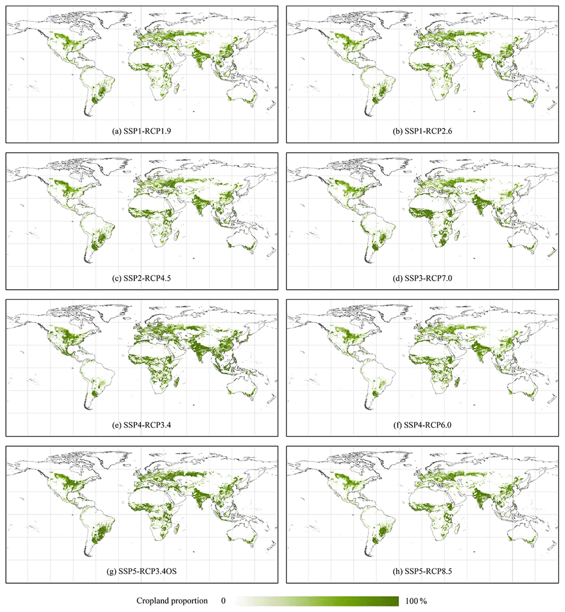
Figure 3Downscaled future cropland maps in 2100 CE under (a) SSP1-RCP1.9, (b) SSP1-RCP2.6, (c) SSP2-RCP4.5, (d) SSP3-RCP7.0, (e) SSP4-RCP3.4, (f) SSP4-RCP6.0, (g) SSP5-RCP3.4OS, and (h) SSP5-RCP8.5.
The overall cropland changes above from the past to the future are interpretable and logical, and they match the qualitative descriptions of cropland changes in some existing studies (Stephens et al., 2019; Ellis et al., 2021; Riahi et al., 2017), indicating the soundness and reliability of our downscaled maps on the whole. To further show the performance of downscaling, we demonstrated some detailed cases (Fig. 4). Several maps at representative time points and places were selected here, including one of the key origin places of agriculture in China (Fig. 4a), European cropland distribution during the Industrial Revolution (Fig. 4b), cropland expansion after the independence of the USA (Fig. 4c), cropland increase in Brazil under SSP1-RCP2.6 (Fig. 4d), African cropland growth under SSP2-RCP4.5 (Fig. 4e), and cropland increase in Southeast Asia under SSP3-RCP7.0 (Fig. 4f). Although these croplands are located in different biophysical and socioeconomic environments, and their types or appearances vary a lot, they are well characterized in our downscaling maps. Visually, our downscaling maps match the spatial patterns in HYDE 3.2 and LUH2 data and reflect more details of cropland distribution. The spatial heterogeneity and field morphology are clearly characterized in our 1 km maps, whereas for the 10 km or 0.25∘ maps, it is hard to maintain some small cropland/non-cropland patches. Furthermore, we took the regions shown in Fig. 4c and f as examples to present and compare the cropland distribution of the same places for different years (Fig. 5) or scenarios (Fig. 6). Figure 5 represents a typical cropland development process in the USA. The cropland changes from past to future in the region are coherently and continuously characterized in our downscaled maps. Both cropland increase and decrease can be accurately tracked, and different change amounts and patterns in different locations are well captured. Figure 6 demonstrates the diverse future cropland development pathways of the region located in Southeast Asia. In our maps, the differences are clearer and vary geographically. Although both regions have varied topography, complex land cover, and fragmented cropland patches, the downscaling results correspond well with HYDE 3.2 and LUH2 and demonstrate fine details in all these different years or scenarios. The detailed demonstrations and comparisons above also prove the importance of developing higher-resolution cropland datasets.

Figure 4Visual comparison between our downscaled maps and HYDE 3.2 and LUH2 for six different areas (a–f). The locations of image center points are as follows: (a) Zhejiang, China (28.338∘ N, 119.321∘ E), (b) Adriatic Sea (43.272∘ N, 14.493∘ E), (c) Kentucky, USA (37.846∘ N, 87.861∘ W), (d) Mato Grosso do Sul, Brazil (19.691∘ S, 54.599∘ W), (e) Koulikoro Region, Mali (12.105∘ N, 8.099∘ W), and (f) Riau, Indonesia (2.199∘ N, 100.425∘ E).
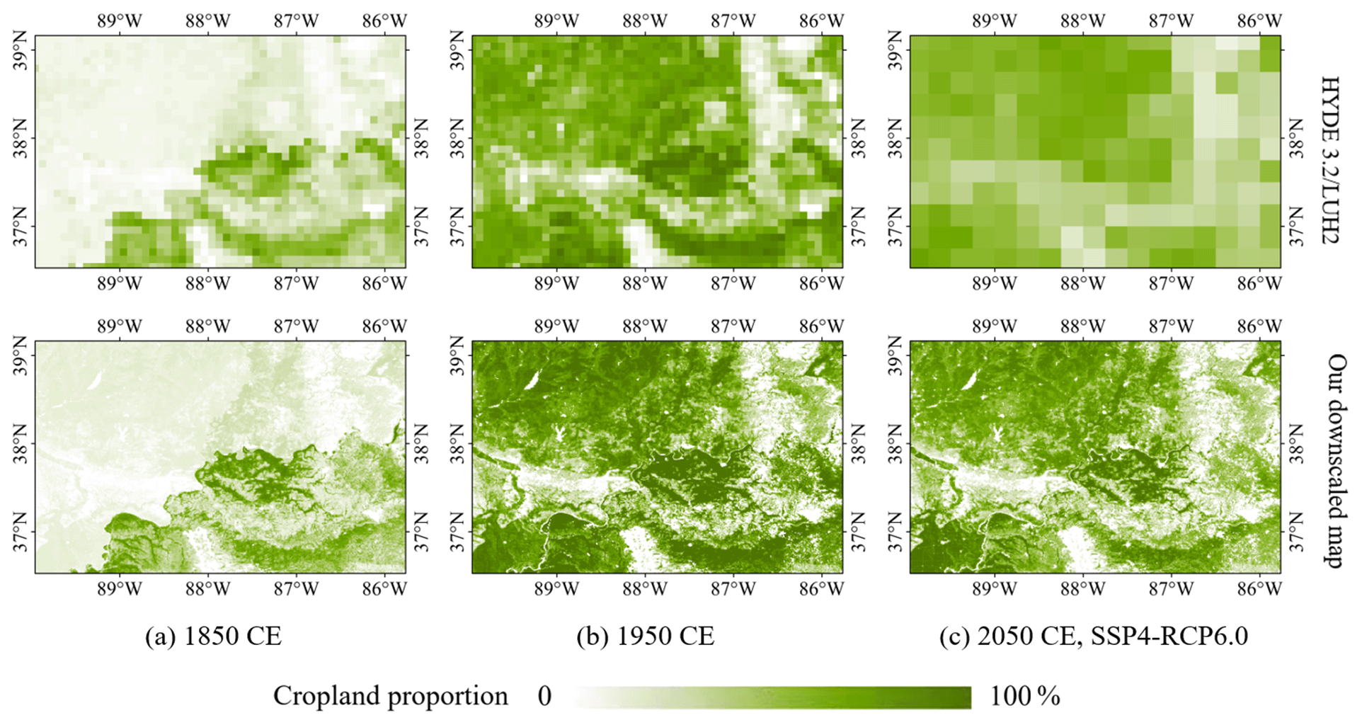
Figure 5Cropland distribution of the region shown in Fig. 4c for different years (a–c). The location of image center points is Kentucky, USA (37.846∘ N, 87.861∘ W).
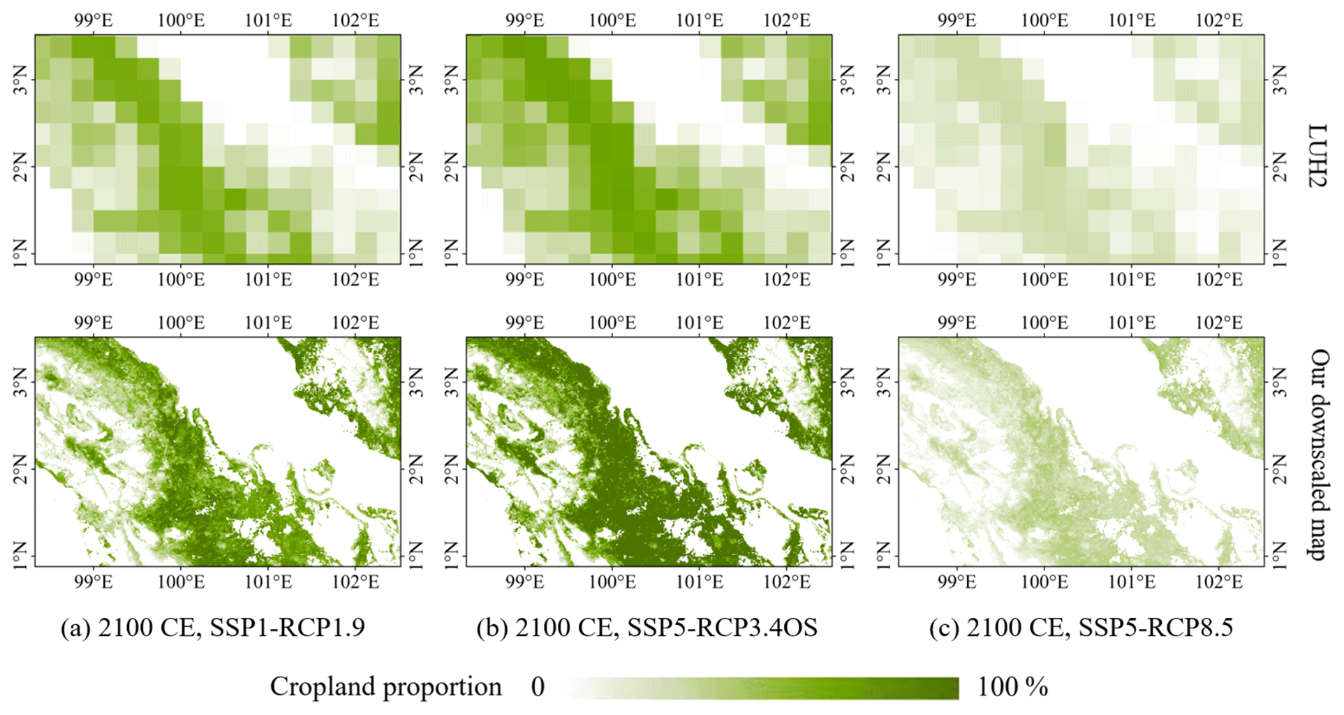
Figure 6Cropland distribution of the region shown in Fig. 4f for different scenarios (a–c). The location of image center points is Riau, Indonesia (2.199∘ N, 100.425∘ E).
Further quantitative comparisons of the spatial distribution between our downscaled cropland data and HYDE 3.2 and LUH2 data are presented in Fig. 7. We aggregated the downscaled maps to align the resolution and calculated the correlation coefficient (r) and the root mean squared error (RMSE) between the corresponding pixels. In general, the datasets exhibited obvious spatial similarity according to the two indicators. For the historical period, the correlation coefficients are usually lower in previous years especially for the pre-1500 CE period because of the discrepancy accumulation over time. However, the RMSEs also decline with downscaling time-step increases (i.e., from present to past), which is mainly attributed to the reduction in cropland proportion in pixels. It should be noted that the RMSE is scale-dependent since it represents absolute differences rather than relative differences. Therefore, direct comparisons of RMSEs between different years/scenarios are actually invalid due to the different scales. For the future period, downscaling performances under different scenarios are distinctive. The most ambitious cropland expansion scenario, SSP4-RCP3.4, displays the minimum consistency. The inconsistencies above are partly influenced by the base map (Fig. 8), and the initial differences transmit into the downscaled maps. The relatively weaker correlations in some years or scenarios do not mean our data are incorrect because our cropland map and HYDE 3.2 and LUH2 use different input data and downscaling strategies. But it can indicate the relatively high uncertainty of results; thus, more future efforts are needed for these time periods or scenarios.
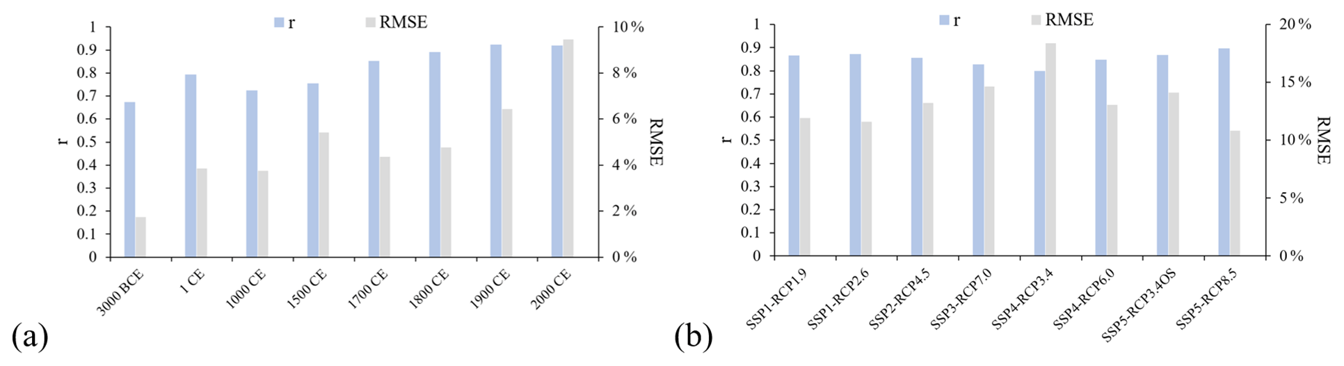
Figure 7Comparison of cropland proportion in the corresponding pixels between our downscaled map and (a) HYDE 3.2 in the eight selected years and (b) LUH2 in 2100 CE under eight future scenarios. Our downscaled maps were aggregated into 10 km and 0.25∘ resolution for the two comparisons, respectively.
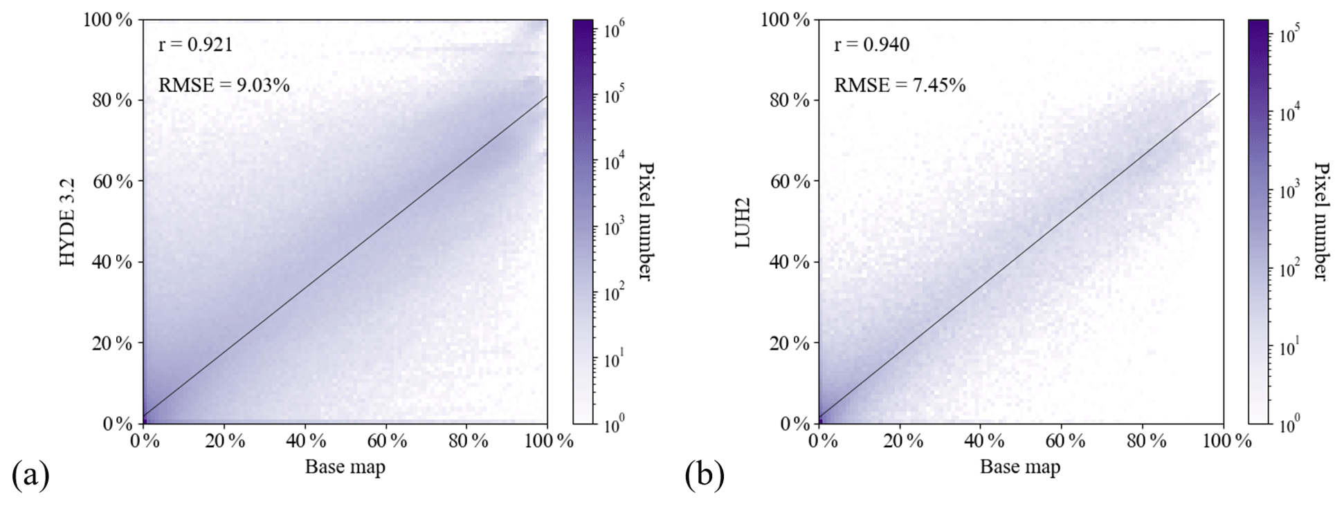
Figure 8Comparison of cropland proportion in the corresponding pixels between the base map and (a) HYDE 3.2 in 2010 CE and (b) LUH2 in 2010 CE. Our downscaled maps were aggregated into 10 km and 0.25∘ resolution for the two comparisons, respectively. The cell value represents the pixel numbers in the corresponding cropland proportion range. The black lines are the linear regression lines.
3.2 Estimated cropland area
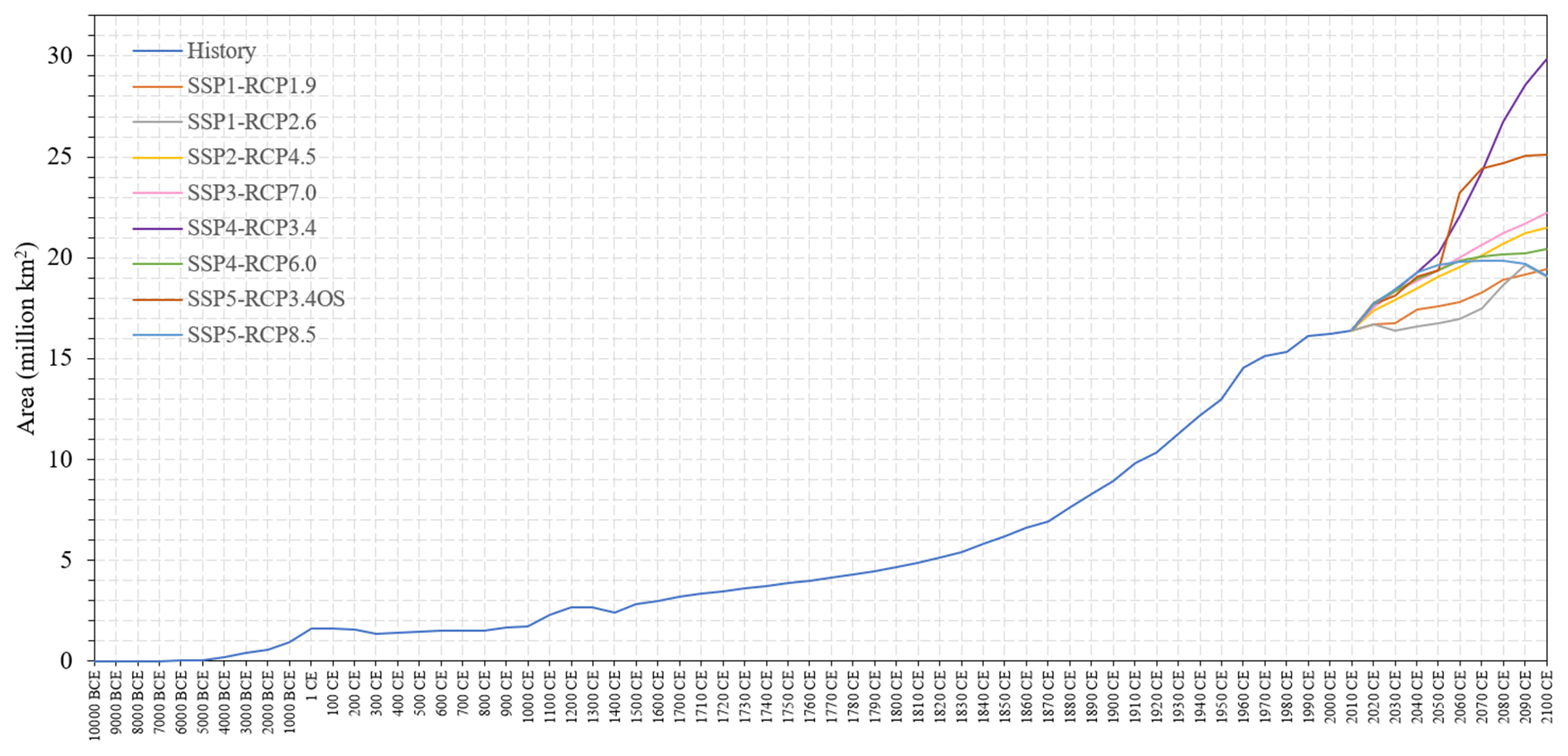
According to our downscaled map, on the whole, global cropland area shows an upward trend from 10 000 BCE to 2100 CE (Fig. 9). It first steadily and constantly increased from the origin of agriculture. In 1500 CE, there was 2.8×10⁶ km2 of cropland globally, and cropland area continuously grew to 6.2×10⁶ km2 by the beginning of large-scale industrialization (∼1850 CE). In the 100 years after 1850 CE, the cropland area increment surpassed that of the past 11 850 years. In recent decades, the growth rate of cropland has slowed down. The area increase in the past 20 years (1990 CE–2010 CE) has been the smallest since the 18th century. In 2010 CE, the global cropland area was 16.4×10⁶ km2. As for the future, the projected cropland areas have substantial discrepancies across the eight SSP-RCP scenarios. Six scenarios (SSP1-RCP1.9, SSP2-RCP4.5, SSP3-RCP7.0, SSP4-RCP3.4, SSP4-RCP6.0, SSP5-RCP3.4OS) yield a monotonously increasing trend with different rates, with the rise ranging from 18.6 % to 82.4 % between 2010 and 2100. The scenario SSP4-RCP3.4 achieves the largest cropland area increment in the 21st century, more than 50 % higher than the scenario with the second-largest increment (SSP5-RCP3.4OS). For scenarios SSP1-RCP2.6 and SSP5-RCP8.5, the turning points are observed in 2090 CE and 2070 CE, respectively, after which cropland area is expected to decline. From 2010 CE to 2100 CE, the increase rate of global cropland area under SSP1-RCP2.6 is 16.4 % and is the smallest.
Additionally, we identified large disparities in the cropland areas among different geographical regions (Fig. 10). Countries around the world were divided into five continents to demonstrate their distinctive agricultural development paths. In the early period, the cropland area was higher and grew steadily in Asia, Europe, and Africa. Before 1850 CE, the total cropland area of these three continents accounts for more than 90 % of global cropland area. By contrast, the cropland area in the Americas and Oceania did not have a substantial increment until the 19th century and the 20th century, respectively. However, after over 200 years of rapid development, the Americas become the second largest continent in agricultural land area. In the last decades, except for the accelerated cropland area rise in Africa, the area tends to be stable in the Americas and Asia and even decreases in Europe and Oceania. In the future, cropland areas in Europe and Oceania will experience the smallest changes in most scenarios (below 0.62×10⁶ km2 and 0.25×10⁶ km2, respectively), whereas cropland in Africa is projected to maintain significant growth under all scenarios (ranging from 43.6 % to 166.4 %). The Americas and Asia demonstrate different development characteristics under different scenarios and are similar to the global trends mentioned above. The historical and future area trajectories across continents track historical pathways and future mitigation policies in different human societies well, and they are connected logically and smoothly.
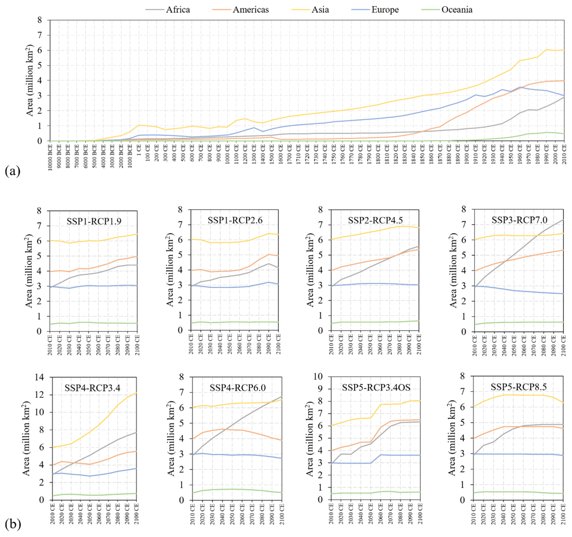
Figure 10Cropland area of different continents for (a) 10 000 BCE–2010 CE and (b) 2010 CE–2100 CE under eight future scenarios. The division of continents is based on countries and is identical to FAO statistics.
To prove the soundness of the results, we also quantitatively compared the cropland area of our dataset with several other datasets (Fig. 11). In years when FAO cropland area statistics (FAO, 2021) were available, our cropland area at continental level was generally consistent in overall patterns with the statistics. The absolute amount of our maps is slightly overestimated for all continents except Europe in several years. The two datasets with full coverage of the entire study period, HYDE 3.2 and LUH2, are taken for the global level comparisons. Our global area time series are highly correlated to them, whereas the RMSE and the regression line indicate our results are slightly higher. The differences above are related to the base map (Fig. 12). However, although FAO data and HYDE and LUH2 data are widely used, they are not completely correct, especially in some developing countries with weak agricultural statistics systems (FAO, 2010). In contrast, our selected base map was produced by the fusion of multilevel cropland area statistics and multiple existing cropland maps. It is more reliable in some regions. But regions with large area differences are still noteworthy, and more area records and surveys are required to reduce the uncertainty.
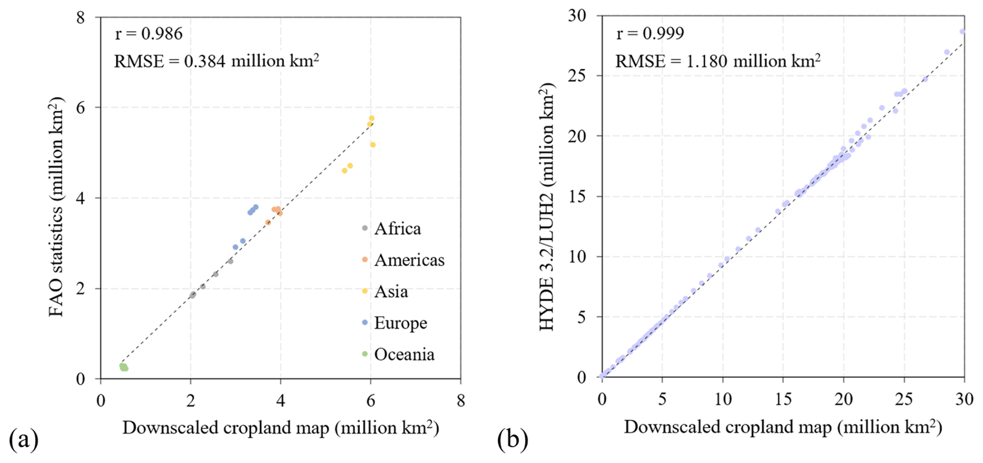
Figure 11Comparison of cropland area between our downscaled map and (a) FAO statistics at the continental level for 1970 CE–2010 CE and (b) HYDE 3.2 and LUH2 at the global level for 10 000 BCE–2100 CE under one historical and eight future scenarios. The black lines are the linear regression lines.
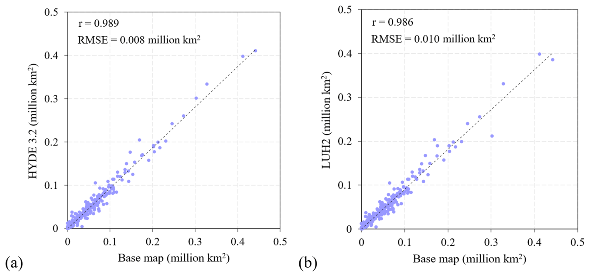
Figure 12Comparison of cropland area at the downscaling region level between the base map and (a) HYDE 3.2 in 2010 CE and (b) LUH2 in 2010 CE. The black lines are the linear regression lines.
Our downscaled dataset provides spatiotemporally continuous and conceptually consistent global cropland distribution information at 1 km resolution, covering the Holocene period until the end of the 21st century. It coincides well with other well-known land use datasets and exhibits superior detailed descriptions. Furthermore, the proposed framework is flexible and efficient, enabling extensions to specific regions or other land use and cover types. However, there are still some limitations and uncertainties in the study, which are expected to be improved by future research.
First, uncertainties in the original demand data (i.e., cropland area of HYDE 3.2 and LUH2) propagated into our downscaled maps. In HYDE 3.2, the total cropland amount for years not covered by FAO statistics (pre-1960 CE period) was determined by modeled population and assumed cropland area per capita curve, which were very uncertain (Klein Goldewijk et al., 2017). The cropland area estimation was very sensitive to them, especially the per capita curve shape. The curve construction cannot capture all specific contexts and special events in regional development. Based on a credibility assessment using historical facts, regional reconstruction results, and expertise, research has pointed out the cropland area estimation errors in some regions such as Northeast China, North China, and some European countries (Fang et al., 2020). In LUH2, the cropland information was derived from IAM simulations. Errors from the simulations attributed to imperfect model structures and assumptions directly affected the cropland area of LUH2 (Riahi et al., 2017). All these inaccurate original demands directly led to harmonized demand errors and poor downscaling performance, especially in some regions where the differences between the original demands and cropland area of the base map were large. Nevertheless, HYDE 3.2 and LUH2 are regarded as authoritative data and are widely used as the basis in related fields despite the limitations above, and there have been no more suitable data to cover such a long time period until now. Moreover, our downscaling work did not focus on simulating the amount of cropland area change but instead spatially disaggregated the given demands to the grid cells. Nevertheless, there is no doubt that more accurate demands help to get better mapping results. If more reliable cropland area data are available in the future, we can update the results based on them.
Second, the initial cropland map caused some limitations. The downscaling results are greatly dependent on the base map. The global synergy map was produced based on a series of cropland datasets with various resolutions. Some input data with coarser resolution affected its accuracy. As a result, cropland percentage in the initial cropland map tends to be overestimated in some high-value pixels and underestimated in some low-value pixels. We also tried other cropland maps extracted from several well-known fine-resolution land cover data products such as GlobeLand30 (Chen et al., 2014), Climate Change Initiative Land Cover (CCI-LC) map (ESA, 2017), and Finer Resolution Observation and Monitoring of Global Land Cover (FROM-GLC) (Gong et al., 2013); however, despite the superior performance in some details, the overall results were even worse. Because of the inconsistent definitions or mapping errors, these satellite-based products generally do not match the statistics and have larger discrepancies with the original demands from HYDE 3.2 and LUH2. Therefore, more future efforts should be made to improve the accuracy of cropland maps.
Third, difficulties of data acquisition in the suitability evaluation hindered the downscaling. We selected some of the most common, widely used, and freely available variables for estimating cropland suitability. Nevertheless, they do not represent all potential factors related to cropland change. Except for the quantity limitations of variables, the quality limitations of these variable data also impact our results. For instance, the imperfect amount estimation and spatial allocation caused uncertainties in population data (Klein Goldewijk et al., 2017). However, there is no better available substitute. Other variables also have their own uncertainties. Here, we quantified the performance of the RF-based suitability evaluation under the variable acquisition limitations. We randomly collected 0.35×10⁶ (accounting for 0.2 % global land pixels at 1 km resolution) test samples worldwide, and we calculated the RMSEs between the 1 km global synergy cropland map and the 1 km suitability layers in 2010 CE. In various WWF biome regions (Fig. 13), the RMSEs are slightly different. At the global scale, the RMSEs are 15.2 % (between the biophysical suitability layer and global synergy cropland map) and 14.7 % (between the biophysical–socioeconomic suitability layer and global synergy cropland map), indicating the suitability evaluation results are acceptable despite the data limitations. Undoubtedly, the performance may get better if more variables with higher quality are accessible. In addition to the variable limitations above, the use of population data with a resolution coarser than 1 km partly limited the ability to depict spatial details especially in the early stage of agricultural development (10 000 BCE–1500 CE). Besides, the biophysical variables were unavailable in years beyond the recent decades and thus remained unchanged for these years in the study. However, using the unchanged variables is the commonly used strategy under data acquisition limitations in land use and cover simulations, and there is no better one. Despite the uncertainties, there is a great demand for complete cropland distribution information throughout the whole process of agricultural development, which is important for the overall understanding of agricultural activities. Compared with HYDE 3.2 and LUH2, we used higher-resolution data and improved methods. Even if for the years beyond the recent decades our maps can still better capture the cropland distribution details and spatial heterogeneity (Figs. 4–6), in the study, we also evaluated the uncertainty for these years, and the results are acceptable (Fig. 7). Nevertheless, to support more precise downscaling, the related driving factor datasets with high resolution and a long time span are urgently needed.
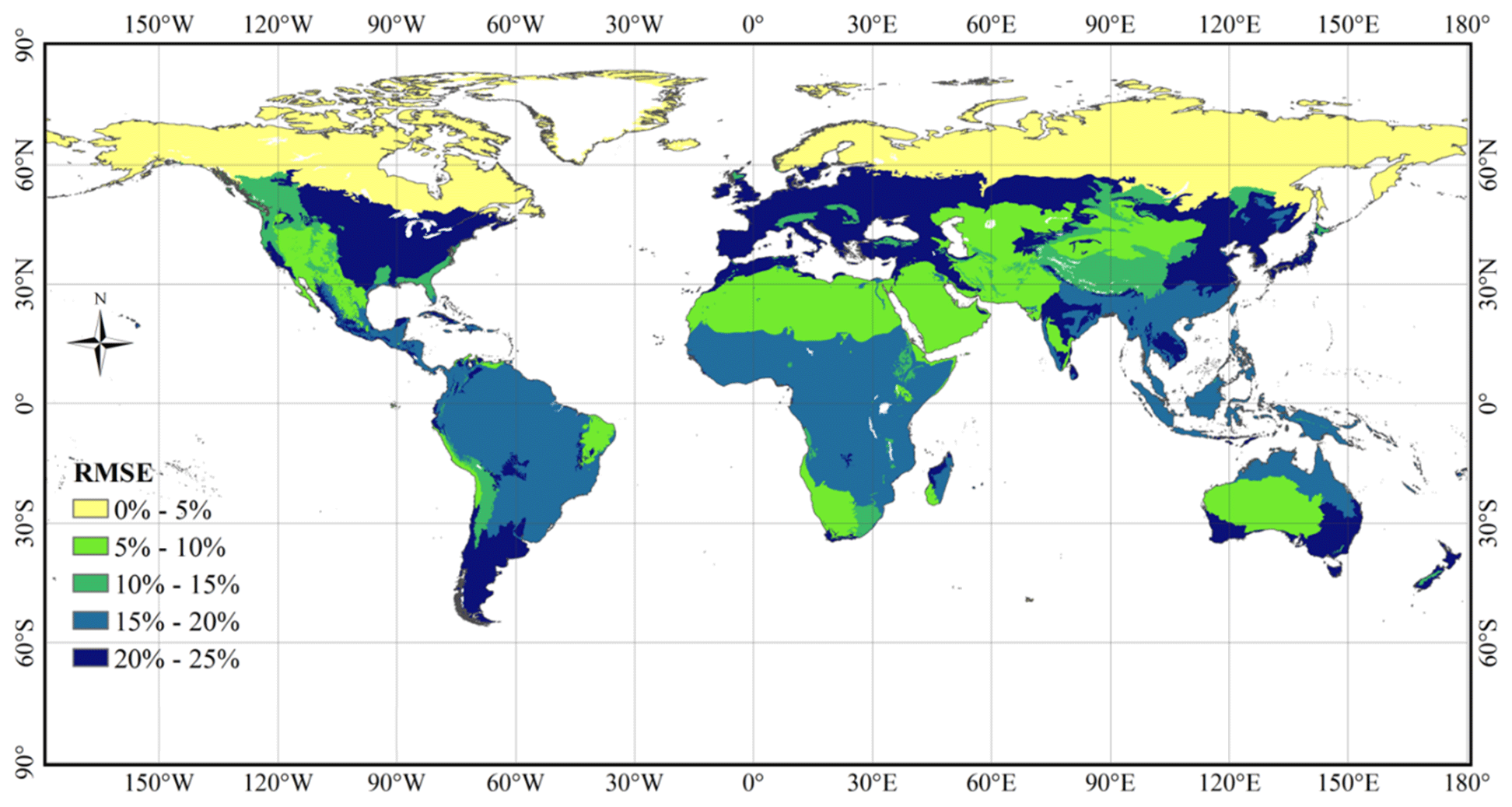
Figure 13Random-forest-based suitability evaluation performance in different WWF biome regions.
Except for the limitations of from input data, others are related to the downscaling model. Some model parameter settings can affect the results, such as moving window size for kernel density calculation. Since the downscaled dataset in the study was developed to provide a globally consistent and coherent spatial distribution of cropland, the parameter setting was based on the situations and rules at the global scale. It did not always incorporate all of the best local data or tune the parameters for local areas especially. Thus, the value set in the study may not be optimal for some regions. As a result, it can be applied at the global scale, whereas it cannot be used as the basis for some local research. But the flexible framework allows researchers to replace input data or revise these model parameters to acquire the best results for their specific study areas. In addition, similar to lots of other prevalent downscaling models, such as CA (Yang et al., 2015), FLUS (Liao et al., 2020), and Demeter (Le Page et al., 2016), our model simulates the cropland within a downscaling region as a whole. If the total cropland area in a downscaling region decreases (increases) at the next time step, it is impossible that local non-cropland (cropland) pixels change to cropland (non-cropland) pixels. As a result, some cropland pixels in historical years that are now non-cropland and some non-cropland pixels in future years that are now cropland cannot be well captured. In the cropland downscaling, one of the typical impacts was that our maps could not characterize well the process of cropland being encroached upon by growing urbanization. Therefore, for further model improvement, in addition to striving to reduce uncertainties in the most sensitive parameters, more process details and additional constraints should be included.
The 1 km global cropland maps for the representative years and scenarios shown in Figs. 2 and 3 are available at https://doi.org/10.5281/zenodo.5105689 (Cao et al., 2021a). The complete 1 km global cropland dataset from 10 000 BCE to 2100 CE can be viewed at https://cbw.users.earthengine.app/view/globalcroplanddataset (Cao et al., 2021c). The map values indicate the proportion of cropland within a 1 km×1 km grid cell.
In the study, the first 1 km resolution global cropland proportion dataset from 10 000 BCE to 2100 CE was produced through the proposed harmonization and downscaling framework. Based on our maps, cropland mainly originated in several independent regions, and it gradually spread to other places at various speeds. Some critical historical events affected the global and regional cropland change. As for the future, the cropland distribution is quite different in various scenarios. Globally, the cropland area has gradually increased over the past years, and it displays distinct trends under eight future scenarios. From 0×106 km2 in 10 000 BCE, it grows to 2.8×10⁶ km2 in 1500 CE, 6.2×10⁶ km2 in 1850 CE, and 16.4×10⁶ km2 in 2010 CE. Between 2010 CE and 2100 CE, the area growth rate ranges from 16.4 % to 82.4 %. In different regions, different natural and socioeconomic conditions lead to obvious spatial heterogeneity. Overall, the distribution and area of our cropland maps are consistent with the existing well-known datasets, and they can better characterize the spatial details compared with these datasets. Some small patches and field morphology are more clearly demonstrated. Limitations of the downscaling originate from the input data and model design, which should be the focus of future research. This high-resolution and long-time-span global cropland dataset can support large-scale earth system simulations or detailed agricultural analysis. The harmonization and downscaling framework can be applied in specific regional/local studies or other land use and cover types through the flexible structure and parameters.
BC and LY conceived the study. BC developed the dataset and analyzed the results with help from LY and XuL. MC, XiL, PH, and PG contributed to the result analysis. BC drafted the manuscript. All authors revised the manuscript.
The contact author has declared that neither they nor their co-authors have any competing interests.
Publisher's note: Copernicus Publications remains neutral with regard to jurisdictional claims in published maps and institutional affiliations.
This research has been supported by the National Key R&D Program of China (grant nos. 2017YFA0604401 and 2019YFA0606601) and the National Key Scientific and Technological Infrastructure project “Earth System Science Numerical Simulator Facility” (EarthLab).
This paper was edited by David Carlson and reviewed by two anonymous referees.
Alexander, P., Prestele, R., Verburg, P. H., Arneth, A., Baranzelli, C., e Silva, F., Brown, C., Butler, A., Calvin, K., Dendoncker, N., Doelman, J. C., Dunford, R., Engstrom, K., Eitelberg, D., Fujimori, S., Harrison, P. A., Hasegawa, T., Havlik, P., Holzhauer, S., Humpenoeder, F., Jacobs-Crisioni, C., Jain, A. K., Krisztin, T., Kyle, P., Lavalle, C., Lenton, T., Liu, J., Meiyappan, P., Popp, A., Powell, T., Sands, R. D., Schaldach, R., Stehfest, E., Steinbuks, J., Tabeau, A., van Meijl, H., Wise, M. A., and Rounsevell, M. D. A.: Assessing uncertainties in land cover projections, Glob. Change Biol., 23, 767–781, https://doi.org/10.1111/gcb.13447, 2017.
Bargiel, D.: A new method for crop classification combining time series of radar images and crop phenology information, Remote Sens. Environ., 198, 369–383, https://doi.org/10.1016/j.rse.2017.06.022, 2017.
Biradar, C. M. and Xiao, X.: Quantifying the area and spatial distribution of double- and triple-cropping croplands in India with multi-temporal MODIS imagery in 2005, Int. J. Remote Sens., 32, 367–386, https://doi.org/10.1080/01431160903464179, 2011.
Breiman, L.: Random forests, Mach. Learn., 45, 5–32, https://doi.org/10.1023/A:1010933404324, 2001.
Cao, B., Yu, L., Li, X., Chen, M., Li, X., Hao, P., and Gong, P.: A 1 km global cropland dataset from 10 000 BCE to 2100 CE, Zenodo [data set], https://doi.org/10.5281/zenodo.5105689, 2021a.
Cao, B., Yu, L., Naipal, V., Ciais, P., Li, W., Zhao, Y., Wei, W., Chen, D., Liu, Z., and Gong, P.: A 30 m terrace mapping in China using Landsat 8 imagery and digital elevation model based on the Google Earth Engine, Earth Syst. Sci. Data, 13, 2437–2456, https://doi.org/10.5194/essd-13-2437-2021, 2021b.
Cao, B., Yu, L., Li, X., Chen, M., Li, X., Hao, P., and Gong, P.: A 1 km global cropland dataset from 10000 BCE to 2100 CE, available at: https://cbw.users.earthengine.app/view/globalcroplanddataset, last access: 8 November 2021c.
Cao, M., Zhu, Y., Quan, J., Zhou, S., Lue, G., Chen, M., and Huang, M.: Spatial Sequential Modeling and Predication of Global Land Use and Land Cover Changes by Integrating a Global Change Assessment Model and Cellular Automata, Earths Future, 7, 1102–1116, https://doi.org/10.1029/2019EF001228, 2019.
Chen, L., Sun, Y., and Sajjad, S.: Monitoring and predicting land use and land cover changes using remote sensing and GIS techniques-A case study of a hilly area, Jiangle, China, PLoS One, 13, e0200493, https://doi.org/10.1371/journal.pone.0200493, 2018.
Chen, J., Ban, Y., and Li, S.: China: Open access to Earth land-cover map, Nature, 514, 434–434, https://doi.org/10.1038/514434c, 2014.
Council, N. R.: Advancing Land Change Modeling: Opportunities and Research Requirements, The National Academies Press, Washington, DC, https://doi.org/10.17226/18385, 2014.
Danielson, J. J. and Gesch, D. B.: Global multi-resolution terrain elevation data 2010 (GMTED2010), Open-File Report, https://doi.org/10.3133/ofr20111073, 2011.
Ellis, E. C., Gauthier, N., Klein Goldewijk, K., Bliege Bird, R., Boivin, N., Díaz, S., Fuller, D. Q., Gill, J. L., Kaplan, J. O., Kingston, N., Locke, H., McMichael, C. N. H., Ranco, D., Rick, T. C., Shaw, M. R., Stephens, L., Svenning, J.-C., and Watson, J. E. M.: People have shaped most of terrestrial nature for at least 12 000 years, P. Natl. Acad. Sci. USA, 118, e2023483118, https://doi.org/10.1073/pnas.2023483118, 2021.
ESA: Land Cover CCI Product User Guide Version 2, available at: https://maps.elie.ucl.ac.be/CCI/viewer/download/ESACCI-LC-Ph2-PUGv2_2.0.pdf (last access: 25 May 2021), 2017.
Estel, S., Kuemmerle, T., Alcántara, C., Levers, C., Prishchepov, A., and Hostert, P.: Mapping farmland abandonment and recultivation across Europe using MODIS NDVI time series, Remote Sens. Environ., 163, 312–325, https://doi.org/10.1016/j.rse.2015.03.028, 2015.
Fang, X., Zhao, W., Zhang, C., Zhang, D., Wei, X., Qiu, W., and Ye, Y.: Methodology for credibility assessment of historical global LUCC datasets, Sci. China Earth Sci., 63, 1013–1025, https://doi.org/10.1007/s11430-019-9555-3, 2020.
FAO: FAOSTAT, available at: http://www.fao.org/faostat/en/#data/RL, last access: 15 May 2021.
FAO: Global Strategy to improve Agricultural and Rural Statistics, available at: http://www.fao.org/3/am082e/am082e00.pdf (last access: 28 May 2021), 2010.
Fick, S. E. and Hijmans, R. J.: WorldClim 2: new 1 km spatial resolution climate surfaces for global land areas, Int. J. Climatol., 37, 4302–4315, https://doi.org/10.1002/joc.5086, 2017.
Foley, J. A., DeFries, R., Asner, G. P., Barford, C., Bonan, G., Carpenter, S. R., Chapin, F. S., Coe, M. T., Daily, G. C., Gibbs, H. K., Helkowski, J. H., Holloway, T., Howard, E. A., Kucharik, C. J., Monfreda, C., Patz, J. A., Prentice, I. C., Ramankutty, N., and Snyder, P. K.: Global consequences of land use, Science, 309, 570–574, https://doi.org/10.1126/science.1111772, 2005.
Friedlingstein, P., O'Sullivan, M., Jones, M. W., Andrew, R. M., Hauck, J., Olsen, A., Peters, G. P., Peters, W., Pongratz, J., Sitch, S., Le Quéré, C., Canadell, J. G., Ciais, P., Jackson, R. B., Alin, S., Aragão, L. E. O. C., Arneth, A., Arora, V., Bates, N. R., Becker, M., Benoit-Cattin, A., Bittig, H. C., Bopp, L., Bultan, S., Chandra, N., Chevallier, F., Chini, L. P., Evans, W., Florentie, L., Forster, P. M., Gasser, T., Gehlen, M., Gilfillan, D., Gkritzalis, T., Gregor, L., Gruber, N., Harris, I., Hartung, K., Haverd, V., Houghton, R. A., Ilyina, T., Jain, A. K., Joetzjer, E., Kadono, K., Kato, E., Kitidis, V., Korsbakken, J. I., Landschützer, P., Lefèvre, N., Lenton, A., Lienert, S., Liu, Z., Lombardozzi, D., Marland, G., Metzl, N., Munro, D. R., Nabel, J. E. M. S., Nakaoka, S.-I., Niwa, Y., O'Brien, K., Ono, T., Palmer, P. I., Pierrot, D., Poulter, B., Resplandy, L., Robertson, E., Rödenbeck, C., Schwinger, J., Séférian, R., Skjelvan, I., Smith, A. J. P., Sutton, A. J., Tanhua, T., Tans, P. P., Tian, H., Tilbrook, B., van der Werf, G., Vuichard, N., Walker, A. P., Wanninkhof, R., Watson, A. J., Willis, D., Wiltshire, A. J., Yuan, W., Yue, X., and Zaehle, S.: Global Carbon Budget 2020, Earth Syst. Sci. Data, 12, 3269–3340, https://doi.org/10.5194/essd-12-3269-2020, 2020.
Fuchs, R., Herold, M., Verburg, P. H., and Clevers, J. G. P. W.: A high-resolution and harmonized model approach for reconstructing and analysing historic land changes in Europe, Biogeosciences, 10, 1543–1559, https://doi.org/10.5194/bg-10-1543-2013, 2013.
Godfray, H. C. J., Beddington, J. R., Crute, I. R., Haddad, L., Lawrence, D., Muir, J. F., Pretty, J., Robinson, S., Thomas, S. M., and Toulmin, C.: Food Security: The Challenge of Feeding 9 Billion People, Science, 327, 812–818, https://doi.org/10.1126/science.1185383, 2010.
Gong, P., Wang, J., Yu, L., Zhao, Y., Zhao, Y., Liang, L., Niu, Z., Huang, X., Fu, H., Liu, S., Li, C., Li, X., Fu, W., Liu, C., Xu, Y., Wang, X., Cheng, Q., Hu, L., Yao, W., Zhang, H., Zhu, P., Zhao, Z., Zhang, H., Zheng, Y., Ji, L., Zhang, Y., Chen, H., Yan, A., Guo, J., Yu, L., Wang, L., Liu, X., Shi, T., Zhu, M., Chen, Y., Yang, G., Tang, P., Xu, B., Giri, C., Clinton, N., Zhu, Z., Chen, J., and Chen, J.: Finer resolution observation and monitoring of global land cover: First mapping results with Landsat TM and ETM+ data, Int. J. Remote Sens., 34, 2607–2654, https://doi.org/10.1080/01431161.2012.748992, 2013.
Grimm, N. B., Faeth, S. H., Golubiewski, N. E., Redman, C. L., Wu, J., Bai, X., and Briggs, J. M.: Global Change and the Ecology of Cities, Science, 319, 756–760, 2008.
Hengl, T.: Soil pH in H2O at 6 standard depths (0, 10, 30, 60, 100 and 200 cm) at 250 m resolution (Version v02), Zenodo [data set], https://doi.org/10.5281/zenodo.1475459, 2018a.
Hengl, T.: Clay content in % (kg/kg) at 6 standard depths (0, 10, 30, 60, 100 and 200 cm) at 250 m resolution (Version v02), Zenodo [data set], https://doi.org/10.5281/zenodo.1476854, 2018b.
Hengl, T. and Gupta, S.: Soil water content (volumetric %) for 33 kPa and 1500 kPa suctions predicted at 6 standard depths (0, 10, 30, 60, 100 and 200 cm) at 250 m resolution (Version v01), Zenodo [data set], https://doi.org/10.5281/zenodo.2629589, 2019.
Hu, Q., Xiang, M., Chen, D., Zhou, J., Wu, W., and Song, Q.: Global cropland intensification surpassed expansion between 2000 and 2010: A spatio-temporal analysis based on GlobeLand30, Sci. Total Environ., 746, 141035, https://doi.org/10.1016/j.scitotenv.2020.141035, 2020.
Hurtt, G. C., Chini, L. P., Frolking, S., Betts, R. A., Feddema, J., Fischer, G., Fisk, J. P., Hibbard, K., Houghton, R. A., Janetos, A., Jones, C. D., Kindermann, G., Kinoshita, T., Klein Goldewijk, K., Riahi, K., Shevliakova, E., Smith, S., Stehfest, E., Thomson, A., Thornton, P., van Vuuren, D. P., and Wang, Y. P.: Harmonization of land-use scenarios for the period 1500–2100: 600 years of global gridded annual land-use transitions, wood harvest, and resulting secondary lands, Clim. Change, 109, 117–161, https://doi.org/10.1007/s10584-011-0153-2, 2011.
Hurtt, G. C., Chini, L., Sahajpal, R., Frolking, S., Bodirsky, B. L., Calvin, K., Doelman, J. C., Fisk, J., Fujimori, S., Klein Goldewijk, K., Hasegawa, T., Havlik, P., Heinimann, A., Humpenöder, F., Jungclaus, J., Kaplan, J. O., Kennedy, J., Krisztin, T., Lawrence, D., Lawrence, P., Ma, L., Mertz, O., Pongratz, J., Popp, A., Poulter, B., Riahi, K., Shevliakova, E., Stehfest, E., Thornton, P., Tubiello, F. N., van Vuuren, D. P., and Zhang, X.: Harmonization of global land use change and management for the period 850–2100 (LUH2) for CMIP6, Geosci. Model Dev., 13, 5425–5464, https://doi.org/10.5194/gmd-13-5425-2020, 2020.
Ito, A. and Hajima, T.: Biogeophysical and biogeochemical impacts of land-use change simulated by MIROC-ES2L, Prog. Earth Planet. Sci., 7, 54, https://doi.org/10.1186/s40645-020-00372-w, 2020.
Kalnay, E. and Cai, M.: Impact of urbanization and land-use change on climate, Nature, 423, 528–531, https://doi.org/10.1038/nature01675, 2003.
Kaplan, J. O., Krumhardt, K. M., Ellis, E. C., Ruddiman, W. F., Lemmen, C., and Klein Goldewijk, K.: Holocene carbon emissions as a result of anthropogenic land cover change, Holocene, 21, 775–791, https://doi.org/10.1177/0959683610386983, 2011.
Klein Goldewijk, K.: Estimating global land use change over the past 300 years: The HYDE Database, Global Biogeochem. Cy., 15, 417–433, https://doi.org/10.1029/1999GB001232, 2001.
Klein Goldewijk, K.: Anthropogenic land-use estimates for the Holocene; HYDE 3.2, DANS [data set], https://doi.org/10.17026/dans-25g-gez3, 2017.
Klein Goldewijk, K. and Verburg, P. H.: Uncertainties in global-scale reconstructions of historical land use: an illustration using the HYDE data set, Landscape Ecol., 28, 861–877, https://doi.org/10.1007/s10980-013-9877-x, 2013.
Klein Goldewijk, K., Beusen, A., and Janssen, P.: Long-term dynamic modeling of global population and built-up area in a spatially explicit way: HYDE 3.1, Holocene, 20, 565–573, https://doi.org/10.1177/0959683609356587, 2010.
Klein Goldewijk, K., Beusen, A., Doelman, J., and Stehfest, E.: Anthropogenic land use estimates for the Holocene – HYDE 3.2, Earth Syst. Sci. Data, 9, 927–953, https://doi.org/10.5194/essd-9-927-2017, 2017.
Le Page, Y., West, T. O., Link, R., and Patel, P.: Downscaling land use and land cover from the Global Change Assessment Model for coupling with Earth system models, Geosci. Model Dev., 9, 3055–3069, https://doi.org/10.5194/gmd-9-3055-2016, 2016.
Li, X., Yu, L., Sohl, T., Clinton, N., Li, W., Zhu, Z., Liu, X., and Gong, P.: A cellular automata downscaling based 1 km global land use datasets (2010–2100), Sci. Bull., 61, 1651–1661, https://doi.org/10.1007/s11434-016-1148-1, 2016.
Li, X., Chen, G., Liu, X., Liang, X., Wang, S., Chen, Y., Pei, F., and Xu, X.: A New Global Land-Use and Land-Cover Change Product at a 1 km Resolution for 2010 to 2100 Based on Human-Environment Interactions, Ann. Am. Assoc. Geogr., 107, 1040–1059, https://doi.org/10.1080/24694452.2017.1303357, 2017.
Liao, W., Liu, X., Xu, X., Chen, G., Liang, X., Zhang, H., and Li, X.: Projections of land use changes under the plant functional type classification in different SSP-RCP scenarios in China, Sci. Bull., 65, 1935–1947, https://doi.org/10.1016/j.scib.2020.07.014, 2020.
Liu, X., Liang, X., Li, X., Xu, X., Ou, J., Chen, Y., Li, S., Wang, S., and Pei, F.: A future land use simulation model (FLUS) for simulating multiple land use scenarios by coupling human and natural effects, Landscape Urban Plan., 168, 94–116, https://doi.org/10.1016/j.landurbplan.2017.09.019, 2017.
Lu, M., Wu, W., You, L., See, L., Fritz, S., Yu, Q., Wei, Y., Chen, D., Yang, P., and Xue, B.: A cultivated planet in 2010 – Part 1: The global synergy cropland map, Earth Syst. Sci. Data, 12, 1913–1928, https://doi.org/10.5194/essd-12-1913-2020, 2020.
Matthews, R. B., Gilbert, N. G., Roach, A., Polhill, J. G., and Gotts, N. M.: Agent-based land-use models: a review of applications, Landscape Ecol., 22, 1447–1459, https://doi.org/10.1007/s10980-007-9135-1, 2007.
Molotoks, A., Stehfest, E., Doelman, J., Albanito, F., Fitton, N., Dawson, T. P., and Smith, P.: Global projections of future cropland expansion to 2050 and direct impacts on biodiversity and carbon storage, Glob. Change Biol., 24, 5895–5908, https://doi.org/10.1111/gcb.14459, 2018.
O'Neill, B. C., Tebaldi, C., van Vuuren, D. P., Eyring, V., Friedlingstein, P., Hurtt, G., Knutti, R., Kriegler, E., Lamarque, J.-F., Lowe, J., Meehl, G. A., Moss, R., Riahi, K., and Sanderson, B. M.: The Scenario Model Intercomparison Project (ScenarioMIP) for CMIP6, Geosci. Model Dev., 9, 3461–3482, https://doi.org/10.5194/gmd-9-3461-2016, 2016.
Olofsson, J. and Hickler, T.: Effects of human land-use on the global carbon cycle during the last 6000 years, Veg. Hist. Archaeobot., 17, 605–615, https://doi.org/10.1007/s00334-007-0126-6, 2008.
Olson, D. M., Dinerstein, E., Wikramanayake, E. D., Burgess, N. D., Powell, G. V. N., Underwood, E. C., D'Amico, J. A., Itoua, I., Strand, H. E., Morrison, J. C., Loucks, C. J., Allnutt, T. F., Ricketts, T. H., Kura, Y., Lamoreux, J. F., Wettengel, W. W., Hedao, P., and Kassem, K. R.: Terrestrial ecoregions of the worlds: A new map of life on Earth, Bioscience, 51, 933–938, https://doi.org/10.1641/0006-3568(2001)051[0933:TEOTWA]2.0.CO;2, 2001.
Pongratz, J., Reick, C., Raddatz, T., and Claussen, M.: A reconstruction of global agricultural areas and land cover for the last millennium, Global Biogeochem. Cy., 22, GB3018, https://doi.org/10.1029/2007GB003153, 2008.
Pongratz, J., Raddatz, T., Reick, C. H., Esch, M., and Claussen, M.: Radiative forcing from anthropogenic land cover change since AD 800, Geophys. Res. Lett., 36, L02709, https://doi.org/10.1029/2008GL036394, 2009.
Poschlod, P., Bakker, J. P., and Kahmen, S.: Changing land use and its impact on biodiversity, Basic Appl. Ecol., 6, 93–98, https://doi.org/10.1016/j.baae.2004.12.001, 2005.
Prestele, R., Alexander, P., Rounsevell, M. D. A., Arneth, A., Calvin, K., Doelman, J., Eitelberg, D. A., Engstrom, K., Fujimori, S., Hasegawa, T., Havlik, P., Humpenoeder, F., Jain, A. K., Krisztin, T., Kyle, P., Meiyappan, P., Popp, A., Sands, R. D., Schaldach, R., Schuengel, J., Stehfest, E., Tabeau, A., Van Meijl, H., Van Vliet, J., and Verburg, P. H.: Hotspots of uncertainty in land-use and land-cover change projections: a global-scale model comparison, Glob. Change Biol., 22, 3967–3983, https://doi.org/10.1111/gcb.13337, 2016.
Prestele, R., Arneth, A., Bondeau, A., de Noblet-Ducoudré, N., Pugh, T. A. M., Sitch, S., Stehfest, E., and Verburg, P. H.: Current challenges of implementing anthropogenic land-use and land-cover change in models contributing to climate change assessments, Earth Syst. Dynam., 8, 369–386, https://doi.org/10.5194/esd-8-369-2017, 2017.
Ramankutty, N. and Foley, J. A.: Estimating historical changes in global land cover: Croplands from 1700 to 1992, Global Biogeochem. Cy., 13, 997–1027, https://doi.org/10.1029/1999GB900046, 1999.
Riahi, K., van Vuuren, D. P., Kriegler, E., Edmonds, J., O'Neill, B. C., Fujimori, S., Bauer, N., Calvin, K., Dellink, R., Fricko, O., Lutz, W., Popp, A., Cuaresma, J. C., Samir, K. C., Leimbach, M., Jiang, L., Kram, T., Rao, S., Emmerling, J., Ebi, K., Hasegawa, T., Havlik, P., Humpenoeder, F., da Silva, L. A., Smith, S., Stehfest, E., Bosetti, V., Eom, J., Gernaat, D., Masui, T., Rogelj, J., Strefler, J., Drouet, L., Krey, V., Luderer, G., Harmsen, M., Takahashi, K., Baumstark, L., Doelman, J. C., Kainuma, M., Klimont, Z., Marangoni, G., Lotze-Campen, H., Obersteiner, M., Tabeau, A., and Tavoni, M.: The Shared Socioeconomic Pathways and their energy, land use, and greenhouse gas emissions implications: An overview, Global Environ. Chang., 42, 153–168, https://doi.org/10.1016/j.gloenvcha.2016.05.009, 2017.
Schaldach, R., Alcamo, J., Koch, J., Kölking, C., Lapola, D. M., Schüngel, J., and Priess, J. A.: An integrated approach to modelling land-use change on continental and global scales, Environ. Modell. Softw., 26, 1041–1051, https://doi.org/10.1016/j.envsoft.2011.02.013, 2011.
Stephens, L., Fuller, D., Boivin, N., Rick, T., Gauthier, N., Kay, A., Marwick, B., Armstrong, C. G., Barton, C. M., Denham, T., Douglass, K., Driver, J., Janz, L., Roberts, P., Rogers, J. D., Thakar, H., Altaweel, M., Johnson, A. L., Vattuone, M. M. S., Aldenderfer, M., Archila, S., Artioli, G., Bale, M. T., Beach, T., Borrell, F., Braje, T., Buckland, P. I., Cano, N. G. J., Capriles, J. M., Castillo, A. D., Çilingiroğlu, Ç., Cleary, M. N., Conolly, J., Coutros, P. R., Covey, R. A., Cremaschi, M., Crowther, A., Der, L., Lernia, S. d., Doershuk, J. F., Doolittle, W. E., Edwards, K. J., Erlandson, J. M., Evans, D., Fairbairn, A., Faulkner, P., Feinman, G., Fernandes, R., Fitzpatrick, S. M., Fyfe, R., Garcea, E., Goldstein, S., Goodman, R. C., Guedes, J. D., Herrmann, J., Hiscock, P., Hommel, P., Horsburgh, K. A., Hritz, C., Ives, J. W., Junno, A., Kahn, J. G., Kaufman, B., Kearns, C., Kidder, T. R., Lanoë, F., Lawrence, D., Lee, G.-A., Levin, M. J., Lindskoug, H. B., López-Sáez, J. A., Macrae, S., Marchant, R., Marston, J. M., McClure, S., McCoy, M. D., Miller, A. V., Morrison, M., Matuzeviciute, G. M., Müller, J., Nayak, A., Noerwidi, S., Peres, T. M., Peterson, C. E., Proctor, L., Randall, A. R., Renette, S., Schug, G. R., Ryzewski, K., Saini, R., Scheinsohn, V., Schmidt, P., Sebillaud, P., Seitsonen, O., Simpson, I. A., Sołtysiak, A., Speakman, R. J., Spengler, R. N., Steffen, M. L., Storozum, M. J., Strickland, K. M., Thompson, J., Thurston, T. L., Ulm, S., Ustunkaya, M. C., Welker, M. H., West, C., Williams, P. R., Wright, D. K., Wright, N., Zahir, M., Zerboni, A., Beaudoin, E., Garcia, S. M., Powell, J., Thornton, A., Kaplan, J. O., Gaillard, M.-J., Goldewijk, K. K., and Ellis, E.: Archaeological assessment reveals Earth's early transformation through land use, Science, 365, 897–902, https://doi.org/10.1126/science.aax1192, 2019.
UNEP-WCMC and IUCN: Protected Planet: The World Database on Protected Areas (WDPA) and World Database on Other Effective Area-based Conservation Measures (WD-OECM), available at: https://www.protectedplanet.net, last access: 25 February 2021.
Veldkamp, A. and Fresco, L. O.: CLUE: A conceptual model to study the conversion of land use and its effects, Ecol. Model., 85, 253–270, https://doi.org/10.1016/0304-3800(94)00151-0, 1996.
Vernon, C., Le Page, Y., Chen, M., Huang, M., Calvin, K., Kraucunas, I., and Braun, C.: Demeter – A Land Use and Land Cover Change Disaggregation Model, J. Open Res. Softw., 6, 15, https://doi.org/10.5334/jors.208, 2018.
Wang, Y., Li, X., Zhang, Q., Li, J., and Zhou, X.: Projections of future land use changes: Multiple scenarios -based impacts analysis on ecosystem services for Wuhan city, China, Ecol. Indic., 94, 430–445, https://doi.org/10.1016/j.ecolind.2018.06.047, 2018.
White, R., Engelen, G., and Uljee, I.: The Use of Constrained Cellular Automata for High-Resolution Modelling of Urban Land-Use Dynamics, Environ. Plann. B, 24, 323–343, https://doi.org/10.1068/b240323, 1997.
Wu, J.: Urban ecology and sustainability: The state-of-the-science and future directions, Landscape Urban Plan., 125, 209–221, https://doi.org/10.1016/j.landurbplan.2014.01.018, 2014.
Xu, Q., Yang, K., Wang, G., and Yang, Y.: Agent-based modeling and simulations of land-use and land-cover change according to ant colony optimization: a case study of the Erhai Lake Basin, China, Nat. Hazards, 75, 95–118, https://doi.org/10.1007/s11069-014-1303-4, 2015.
Yang, X., Jin, X., Guo, B., Long, Y., and Zhou, Y.: Research on reconstructing spatial distribution of historical cropland over 300 years in traditional cultivated regions of China, Global Planet. Change, 128, 90–102, https://doi.org/10.1016/j.gloPlacha.2015.02.007, 2015.
Yu, L., Wang, J., Clinton, N., Xin, Q., Zhong, L., Chen, Y., and Gong, P.: FROM-GC: 30 m global cropland extent derived through multisource data integration, Int. J. Digit. Earth, 6, 521–533, https://doi.org/10.1080/17538947.2013.822574, 2013.
Yu, L., Wang, J., Li, X., Li, C., Zhao, Y., and Gong, P.: A multi-resolution global land cover dataset through multisource data aggregation, Sci. China Earth Sci., 57, 2317–2329, https://doi.org/10.1007/s11430-014-4919-z, 2014.
Yu, L., Fu, H., Wu, B., Clinton, N., and Gong, P.: Exploring the potential role of feature selection in global land-cover mapping, Int. J. Remote Sens., 37, 5491–5504, https://doi.org/10.1080/01431161.2016.1244365, 2016.
Yu, Z. and Lu, C.: Historical cropland expansion and abandonment in the continental US during 1850 to 2016, Global Ecol. Biogeogr., 27, 322–333, https://doi.org/10.1111/geb.12697, 2018.
Zabel, F., Delzeit, R., Schneider, J. M., Seppelt, R., Mauser, W., and Václavík, T.: Global impacts of future cropland expansion and intensification on agricultural markets and biodiversity, Nat. Commun., 10, 2844, https://doi.org/10.1038/s41467-019-10775-z, 2019.
Zhong, L., Gong, P., and Biging, G. S.: Efficient corn and soybean mapping with temporal extendability: A multi-year experiment using Landsat imagery, Remote Sens. Environ., 140, 1–13, https://doi.org/10.1016/j.rse.2013.08.023, 2014.