the Creative Commons Attribution 4.0 License.
the Creative Commons Attribution 4.0 License.
 | 23 Feb 2021
A 6-year-long (2013–2018) high-resolution air quality reanalysis dataset in China based on the assimilation of surface observations from CNEMC
Xiao Tang
Jiang Zhu
Zifa Wang
Jianjun Li
Huangjian Wu
Qizhong Wu
Huansheng Chen
Lili Zhu
Wei Wang
Bing Liu
Qian Wang
Duohong Chen
Yuepeng Pan
Tao Song
Fei Li
Haitao Zheng
Guanglin Jia
Miaomiao Lu
Lin Wu
Gregory R. Carmichael
A 6-year-long high-resolution Chinese air quality reanalysis (CAQRA) dataset is presented in this study obtained from the assimilation of surface observations from the China National Environmental Monitoring Centre (CNEMC) using the ensemble Kalman filter (EnKF) and Nested Air Quality Prediction Modeling System (NAQPMS).This dataset contains surface fields of six conventional air pollutants in China (i.e. PM2.5, PM10, SO2, NO2, CO, and O3) for the period 2013–2018 at high spatial (15 km×15 km) and temporal (1 h) resolutions. This paper aims to document this dataset by providing detailed descriptions of the assimilation system and the first validation results for the above reanalysis dataset. The 5-fold cross-validation (CV) method is adopted to demonstrate the quality of the reanalysis. The CV results show that the CAQRA yields an excellent performance in reproducing the magnitude and variability of surface air pollutants in China from 2013 to 2018 (CV R2=0.52–0.81, CV root mean square error (RMSE) =0.54 for CO, and CV RMSE =16.4–39.3 for the other pollutants on an hourly scale). Through comparison to the Copernicus Atmosphere Monitoring Service reanalysis (CAMSRA) dataset produced by the European Centre for Medium-Range Weather Forecasts (ECWMF), we show that CAQRA attains a high accuracy in representing surface gaseous air pollutants in China due to the assimilation of surface observations. The fine horizontal resolution of CAQRA also makes it more suitable for air quality studies on a regional scale. The PM2.5 reanalysis dataset is further validated against the independent datasets from the US Department of State Air Quality Monitoring Program over China, which exhibits a good agreement with the independent observations (R2=0.74–0.86 and RMSE =16.8–33.6 in different cities). Furthermore, through the comparison to satellite-estimated PM2.5 concentrations, we show that the accuracy of the PM2.5 reanalysis is higher than that of most satellite estimates. The CAQRA is the first high-resolution air quality reanalysis dataset in China that simultaneously provides the surface concentrations of six conventional air pollutants, which is of great value for many studies, such as health impact assessment of air pollution, investigation of air quality changes in China, model evaluation and satellite calibration, optimization of monitoring sites, and provision of training data for statistical or artificial intelligence (AI)-based forecasting. All datasets are freely available at https://doi.org/10.11922/sciencedb.00053 (Tang et al., 2020a), and a prototype product containing the monthly and annual means of the CAQRA dataset has also been released at https://doi.org/10.11922/sciencedb.00092 (Tang et al., 2020b) to facilitate the evaluation of the CAQRA dataset by potential users.
- Article
(19368 KB) - Full-text XML
- BibTeX
- EndNote


Air pollution is a critical environmental issue that adversely affects human health and is closely connected to climate change (von Schneidemesser et al., 2015). Exposure to ambient air pollution has been confirmed by many epidemiological studies to be a leading contributor to the global disease burden, which increases both morbidity and mortality (Cohen et al., 2017). China, as the largest developing country, has achieved great economic development since the 1980s. This large-scale economic expansion, however, is accompanied by a dramatic increase in air pollutant emissions, leading to severe air pollution in China (Kan et al., 2012). Since 2012, the Chinese government has established a nationwide ground-based air quality monitoring network (Fig. 1) to monitor the surface concentrations of six conventional air pollutants in China – i.e. particles with an aerodynamic diameter of 2.5 µm or smaller (PM2.5), particles with an aerodynamic diameter of 10 µm or smaller (PM10), sulfur dioxide (SO2), nitrogen dioxide (NO2), carbon monoxide (CO), and ozone (O3) – which plays an irreplaceable role in understanding the air pollution in China. In addition, since the implementation of the Action Plan for the Prevention and Control of Air Pollution in 2013, a series of aggressive control measures have been applied in China to reduce the emissions of air pollutants. According to the estimates of Zheng et al. (2018b), Chinese anthropogenic emissions have decreased by 59 % for SO2, 21 % for NOx, 23 % for CO, 36 % for PM10, and 35 % for PM2.5 from 2013 to 2017. Concurrently, the air quality in China has changed dramatically over the past 6 years (Silver et al., 2018; Zheng et al., 2017). Such large changes in Chinese air quality and their effects on human health and the environment have become an increasingly hot topic in many scientific fields (e.g. Xue et al., 2019; Zheng et al., 2017), necessitating a long-term air quality dataset in China with high accuracy and spatiotemporal resolutions.
Ground-based observations can provide accurate information on the spatial and temporal distributions of air pollutants in China, but they are sparsely and unevenly distributed in space. Satellite observations exhibit the advantages of a high spatial coverage and have widely been applied in air pollution monitoring over large domains. A series of satellite retrievals related to air quality have been developed over the past 2 decades, such as the observations of NO2, SO2, and O3 columns from the Ozone Monitoring Instrument (OMI; Levelt et al., 2006), CO column observations from the Measurement of Pollution in the Troposphere (MOPITT; Deeter et al., 2003), and aerosol optical depth (AOD) observations from the Moderate Resolution Imaging Spectroradiometer (MODIS; Barnes et al., 1998). These satellite column measurements have also been used to estimate surface concentrations based on different methods, such as chemical transport models (CTMs) (e.g. van Donkelaar et al., 2016, 2010), advanced statistical methods (e.g. Ma et al., 2014, 2016; Xue et al., 2019; Zou et al., 2017), and semi-empirical models (e.g. Lin et al., 2015, 2018), which have been proven to be an effective way to acquire wide-coverage distributions of surface air pollutant with good accuracy (Chu et al., 2016; Shin et al., 2019). However, challenges remain in satellite-based estimates due to missing values related to cloud contamination, uncertainties in satellite measurements, and difficulties in modelling the complex relationship between surface concentrations and column measurements (Shin et al., 2019; van Donkelaar et al., 2016; Xue et al., 2019). In addition, most satellite-based estimates of surface concentrations exhibit low temporal resolutions (daily or even longer), which limit their application in fine-scale studies, such as the assessment of the acute health effects of the air quality. To our knowledge, a nationwide long-term estimate of the surface concentrations of all conventional air pollutants in China on an hourly scale have not yet been reported in previous satellite estimates.
A long-term air quality reanalysis dataset of critical air pollutants can provide constrained estimates of their concentrations at all locations and times, which optimally combines the accuracy of observations and the physical information and spatial continuity of CTMs through advanced data assimilation techniques. Reanalysis datasets are uniform, continuous, and state-of-the-science best-estimate data products that have been adopted by a vast number of research communities. For example, several long-term meteorological reanalysis datasets have been developed by various weather centres in different regions and countries, such as the ERA-Interim reanalysis developed by the European Centre for Medium-Range Weather Forecasts (ECMWF; Dee et al., 2011), the National Center for Atmospheric Research (NCAR)/National Centers for Environmental Protection (NCEP) reanalysis developed by the NCEP (Saha et al., 2010), the Modern-Era Retrospective Analysis for Research and Applications (MERRA) developed by the NASA Global Modeling and Assimilation Office (NASA-GMAO; Rienecker et al., 2011), the Japanese 55-year Reanalysis (JRA-55) developed by the Japan Meteorological Agency (Kobayashi et al., 2015), and the China Meteorological Administration's Global Atmospheric Reanalysis (CRA-40) developed by the China Meteorological Administration (CMA). The use of data assimilation in atmospheric chemistry reanalysis is more recent, and certain reanalysis datasets for atmospheric composition have been produced over the past decades, for example the Monitoring Atmospheric Composition and Climate (MACC), Copernicus Atmosphere Monitoring Service (CAMS) interim reanalysis (CIRA), and CAMS reanalysis (CAMSRA) produced by the ECWMF (Flemming et al., 2017; Inness et al., 2019, 2013); the MERRA-2 aerosol reanalysis produced by the NASA-GMAO (Randles et al., 2017); the tropospheric chemistry reanalysis (TCR) from 2005–2012 produced by Miyazaki et al. (2015) and its latest version TCR-2 (Miyazaki et al., 2020); the global reanalysis of carbon monoxide produced by Gaubert et al. (2016); the multi-sensor total ozone reanalysis from 1970–2012 produced by van der A et al. (2015); and the Japanese Reanalysis for Aerosols (JRAero) from 2011–2015 produced by Yumimoto et al. (2017). These reanalysis datasets promote our understanding of atmospheric composition and also facilitate air quality research. However, these datasets are all global datasets with coarse horizonal resolutions (>50 km), which may be insufficient to capture the high spatial variability of air pollutants on a regional scale. In addition, some of these reanalysis datasets only provide air quality data prior to the year 2012 and only focus on specific species. There is still no high-resolution air quality reanalysis dataset in China capturing its dramatic air quality change during recent years.
In view of these discrepancies, in this study we develop a high-resolution regional air quality reanalysis dataset in China from 2013 to 2018 (which will be extended in the future on a yearly basis) by assimilating surface observations from the China National Environmental Monitoring Centre (CNEMC). The developed reanalysis dataset may help mitigate the lack of high-resolution air quality datasets in China by providing surface concentration fields of all six conventional air pollutants in China at high spatial (15 km×15 km) and temporal (hourly) resolutions, which is of great value to (1) retrospective air quality analysis in China, (2) health and environmental impact assessment of air pollution on fine scales, (3) model evaluation and satellite calibration, (4) optimization of monitoring sites, and (5) provision of basic training datasets for statistical or artificial intelligence (AI)-based forecasting.
The Chinese air quality reanalysis (CAQRA) dataset was produced with the chemical data assimilation system (ChemDAS) developed by the Institute of Atmospheric Physics, Chinese Academy of Sciences (IAP, CAS) (Tang et al., 2011). This system consists of (i) a three-dimensional CTM called the Nested Air Quality Prediction Modeling System (NAQPMS) developed by Wang et al. (2000), (ii) an ensemble Kalman filter (EnKF) assimilation algorithm, and (iii) surface observations from CNEMC with the automatic outlier detection method developed by Wu et al. (2018). We adopted an offline analysis scheme in this study since there are no previous experiences with online chemical data assimilation at such a high horizontal resolution. The lessons learnt from this offline analysis application could also facilitate future implementation of online analysis. In the offline analysis scheme, a free ensemble simulation is first conducted, and the observations are then assimilated using the EnKF. A similar offline analysis scheme has also been applied in previous reanalysis studies, such as Candiani et al. (2013) and Kumar et al. (2012). Detailed descriptions of the ensemble simulation, observations, and data assimilation algorithm used in this study are presented below.
2.1 Air pollution prediction model
The NAQPMS model was used as the forecast model to represent the atmospheric chemistry, which has been applied in previous assimilation studies (Tang et al., 2011, 2013). The model is driven by the hourly meteorological fields produced by the Weather Research and Forecasting (WRF) model (Skamarock, 2008). Gas phase chemistry is simulated with the carbon bond mechanism Z developed by Zaveri and Peters (1999). Aqueous-phase chemistry and wet deposition are simulated based on the Regional Acid Deposition Model (RADM) mechanism in the Community Multi-scale Air Quality (CMAQ) model version 4.6. In regard to aerosol processes, the thermodynamic model ISORROPIA 1.7 (Nenes et al., 1998) is applied for the simulations of inorganic atmospheric aerosols. Six secondary organic aerosols are explicitly treated in the NAQPMS model based on Li et al. (2011). To simulate the interactions between particles and gases, 28 heterogeneous reactions involving sulfate, soot, dust, and sea salt particles are included based on previous studies (Li et al., 2015, 2012). Size-resolved mineral dust emissions are calculated online as a function of the relative humidity, frictional velocity, mineral particle size distribution, and surface roughness (Li et al., 2012). Sea salt emissions are calculated with the scheme of Athanasopoulou et al. (2008). The dry deposition of gases and aerosols is modelled based on the scheme of Wesely (1989), and advection is simulated with the accurate mass conservation algorithm of Walcek and Aleksic (1998).
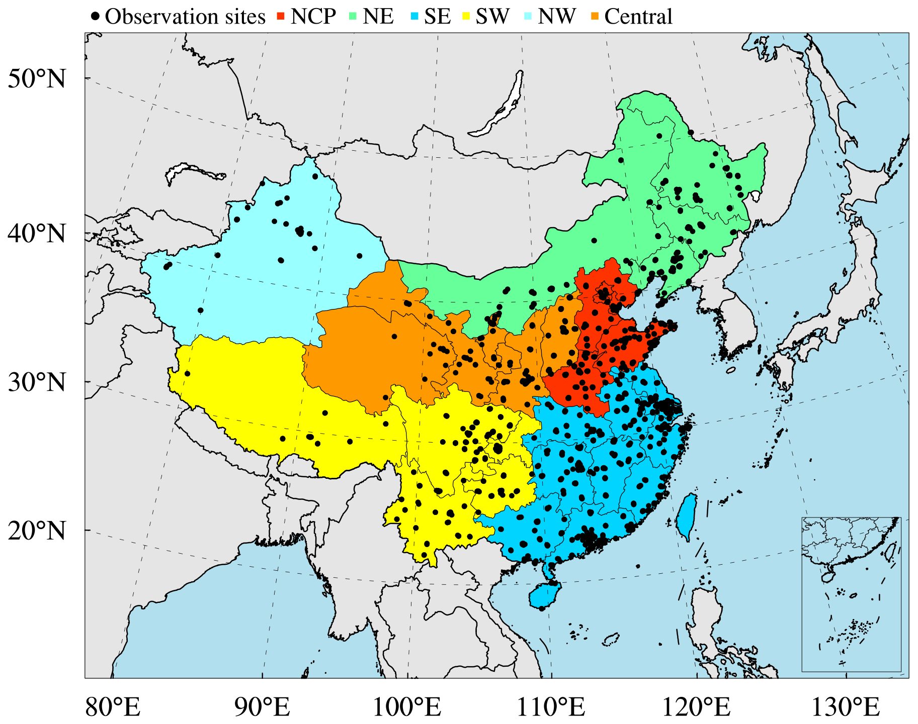
Figure 1Modelling domain of the ensemble simulation overlain on the distribution of the observation sites of the CNEMC. The different colours denote the different regions in China, namely, the North China Plain (NCP), northeast China (NE), southwest China (SW), southeast China (SE), northwest China (NW), and central China.
Figure 1 shows the modelling domain of this study, which covers most parts of East Asia with a fine horizontal resolution of 15 km. The vertical coordinate system consists of 20 terrain-following levels, with the model top reaching up to 20 000 m and the first layer at approximately 50 m. Nine vertical layers are set within 2 km of the surface to better characterize the vertical mixing process within the boundary layers. The emissions of air pollutants considered in this study include the monthly anthropogenic emissions retrieved from the Hemispheric Transport of Air Pollution (HTAP) v2.2 emission inventory with a base year of 2010 (Janssens-Maenhout et al., 2015), biomass burning emissions retrieved from the Global Fire Emissions Database (GFED) version 4 (Randerson et al., 2017; van der Werf et al., 2010), biogenic volatile organic compound (BVOC) emissions retrieved from the Model of Emissions of Gases and Aerosols from Nature (MEGAN)-MACC (Sindelarova et al., 2014), marine VOC emissions retrieved from the POET database (Granier et al., 2005), soil NOx emissions retrieved from the Regional Emission Inventory in Asia (Yan et al., 2003), and lightning NOx emissions retrieved from Price et al. (1997). Clean initial conditions are used in the air quality simulations with a 2-week free run of the NAQPMS model as the spin-up time. The top and boundary conditions are provided by the Model for Ozone and Related Chemical Tracers (MOZART; Brasseur et al., 1998; Hauglustaine et al., 1998) model, and the meteorological fields are provided by the WRF model. In each daily meteorology simulation, a 36 h free run of the WRF model is conducted with the first 12 h simulation period as the spin-up run and the remaining 24 h period providing the meteorologic inputs for the NAQPMS model. The initial and boundary conditions for the meteorology simulations are provided by the NCAR/NCEP 1∘ × 1∘ reanalysis data.
Table 1Uncertainties in the emissions of the different species.
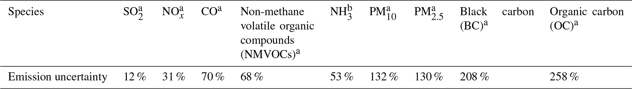
a Emission uncertainty obtained from Zhang et al. (2009). b Emission uncertainty obtained from Streets et al. (2003).
2.2 Generation of ensemble simulation
The EnKF uses an ensemble of model simulation to represent the forecast uncertainty, which should include the most model uncertain aspects. Considering that the emissions are a major source of uncertainty in air quality prediction (Carmichael et al., 2008; Hanna et al., 1998; M. Li et al., 2017), in this study the ensemble was generated by perturbing the emissions based on their error probability distribution functions (PDFs), which were assumed to be Gaussian distributions. Table 1 lists the perturbed species considered in this study as well as their corresponding emission uncertainties obtained from previous studies. The perturbed emissions were parameterized by multiplying the base emissions with a perturbation factor β, as expressed in Eq. (1):
where E denotes the vector of base emissions, ∘ denotes the Schur product, and N denotes the ensemble size. The performance of the EnKF is strongly related to the ensemble size, which determines the accuracy to which the background error covariance is approximated (Constantinescu et al., 2007; Miyazaki et al., 2012). A large ensemble size is important in capturing the proper background error covariance structure, especially in high-resolution data assimilation application due to the fine-scale variability and large degree of freedoms. However, a large ensemble is computationally expensive as the cost of EnKF linearly increases with ensemble size, while the accuracy of covariance estimate improves by its square root (Constantinescu et al., 2007). Thus, an appropriate ensemble should keep a good balance between accuracy and computational cost. Constantinescu et al. (2007) in their ideal experiments showed that a 50-member ensemble has significant improvement against smaller ensembles, and Miyazaki et al. (2012) in their real chemical assimilation experiments showed that the improvement was much less significant by further increasing the ensemble size from 48 to 64. Thus, the ensemble size was chosen as 50 in this study by referencing pervious publications and also our previous high-resolution regional assimilation work (Tang et al., 2011, 2013, 2016), which showed that a 50-member ensemble keeps good balance between assimilation performance and computational efficiency. However, it should be noted that our application has higher horizontal resolution than that of Constantinescu et al. (2007) and Miyazaki et al. (2012), which may require a larger ensemble size due to the larger degrees of freedom in our application. Thus, to reduce the degrees of freedom in our high-resolution data assimilation work, we assumed that the emission errors were spatially correlated, and an isotropic correlation model was assumed in the covariance of the emission errors, which is written as
where ρ(i,j) represents the correlation between grids i and j; h(i,j) is the distance between these two points; and l is the decorrelation length, which was specified as 150 km in this study. According to the PDF of the emission errors, β follows the same Gaussian distribution as the emission errors except that its mean equals 1. Using the method of Evensen (1994), 50 smooth pseudo-random perturbation fields of β were generated for each perturbed species. In addition, the emission perturbations were kept independent from each other to prevent pseudo-correlation among the different species.
2.3 Observations
Surface observations of the hourly ambient PM2.5, PM10, SO2, NO2, CO, and O3 concentrations retrieved from the CNEMC were used in this study. The number of observation sites was approximately 510 in 2013 and increased to 1436 in 2015. Real-time observations of these six air pollutants at each monitoring site are routinely gathered by the CNEMC and released to the public (available at http://www.cnemc.cn/; last access: 17 April 2020) at hourly intervals. A challenge that should be overcome in the assimilations of surface observation is that there are occasional outliers occurring in these observations due to the instrument malfunctions, influences of harsh environments, and limitations of the measurement method. Filtering out these outliers is necessary before the assimilation; otherwise these outliers may cause unrealistic spatial and temporal variations in the reanalysis. To address this issue, a fully automatic outlier detection method was developed by Wu et al. (2018) to filter out the observation outliers. An automatic outlier detection method is very important in chemical data assimilation since there is a large amount of observation data on multiple species. Four types of outliers – characterized by temporal and spatial inconsistencies, instrument-induced low variances, periodic calibration exceptions, and lower PM10 concentrations than those of PM2.5 – were detected and removed before the assimilation. Figure A1 in Appendix A shows the removal ratios of the six air pollutants from 2013 to 2018, which are generally around 1.5 % for most air pollutants throughout the assimilation period. The PM10 observations have a high removal ratio (9–13 %) during 2013–2015, with most of these outliers marked by lower PM10 concentrations than those of PM2.5. However, there was a sharp decrease in removal ratios of PM10 in 2016 (∼1.5 %) because of the implementation of a compensation algorithm for the loss of semi-volatile materials in the PM10 measurements (Wu et al., 2018). To assess the potential impacts of outlier detection on the assimilations, the differences in annual concentrations caused by quality control are shown in Fig. A2. The differences were generally positive for PM2.5, SO2, NO2, and CO concentrations, indicating a lower tendency of these species' concentrations due to the use of outlier detection. Negative differences were mainly found in the PM10 concentrations in south China and the O3 concentrations throughout China. According to estimation, the impacts of outlier detection were generally small at most stations. The differences were less than 5 (1 ) for PM2.5 concentrations over most stations in north (south) China and less than 1 for the gaseous air pollutants for most stations throughout China. The differences were shown to be relative larger for PM10 concentrations over northwest (NW) China, which can be over 20 at stations around the Taklimakan Desert. This would be due to the higher outlier ratios in the observations over the remote areas. More details on the outlier detection method are available in Wu et al. (2018).
A proper estimate of the observation error is important in regard to the filter performance since the observation and background errors determine the relative weights of the observation and background values in the analysis. The observation error includes measurement and representativeness errors. For each species, the measurement error was given by its respective instruments, namely, 5 % for PM2.5 and PM10; 2 % for SO2, NO2, and CO; and 4 % for O3 according to officially released documents of the Chinese Ministry of Ecology and Environmental Protection (HJ 193–2013 and HJ 654–2013, available at http://www.cnemc.cn/jcgf/dqhj/; last access: 17 April 2020). The representativeness error arises from the different spatial scales that the gridded model results and discrete observations represent, which is parameterized by the formula proposed by Elbern et al. (2007) in this study:
where rrepr represents the representativeness error, Δx represents the model resolution, Lrepr represents the characteristic representativeness length of the observation site, and εabs represents the error characteristic parameters for different species. The estimation of Lrepr is dependent on the types of observation sites, with urban sites usually having smaller representative length than the rural sites have due to the larger representativeness errors. Considering that the observation sites from CNEMC were almost all city (urban) sites (>90 %), the Lrepr was assigned to be 2 km in this study according to Elbern et al. (2007).
For the estimations of εabs, previous studies (D. Chen et al., 2019; Feng et al., 2018; Jiang et al., 2013; Ma et al., 2019; Pagowski and Grell, 2012; Peng et al., 2017; Werner et al., 2019) usually assigned the εabs empirically to be half of the measurement error following the study by Pagowski et al. (2010). In this study, the εabs was obtained from F. Li et al. (2019), who estimated the εabs based on a dense observation network in the Beijing–Tianjin–Hebei region. In their study, the representativeness error of each species' observation was first estimated by the spatiotemporally averaged standard deviation of the observed values within a 30 km×30 km grid:
where rrepr,i represents the representativeness errors of the observations for species i; represents the standard deviation of the observed values of species i at different sites that are located in the same grid m at time t; and M and T represent the total number of grids and observation time, respectively. After the estimations of rrepr,i, the for species i were estimated by a transformation of Eq. (3):
where Δx is equal to 30 km. Based on the estimated Lrepr,i and the for different species, the representativeness errors are estimated using Eq. (3) by specifying the Δx to be 15 km.
2.4 Data assimilation algorithm
We used a variant of the EnKF approach, i.e. the local ensemble transform Kalman filter (LETKF; Hunt et al., 2007), to assimilate the observations into the model state. The LETKF has several advantages over the original EnKF (e.g. Miyazaki et al., 2012). As a kind of deterministic filter, it does not need to perturb the observations, which avoids introducing additional sampling errors. In addition, the LETKF performs the analysis locally in space and time, which not only alleviates the rank problem of the EnKF method but also suppresses the spurious long-distance correlation caused by the limited ensemble size. The formulation of the LETKF can be written as
where is the analysis state, is the background state, Xb represents the background perturbations, is the analysis in the ensemble space spanned by Xb, is the analysis error covariance in the ensemble space with dimensions of Nens×Nens, yo is the vector of observations used in the analysis of this grid, R is the observation error covariance matrix, and H is the linear observational operator that maps the model space to the observation space. The scalar λ in Eq. (8) denotes the inflation factor for the background covariance matrix, which was estimated with the algorithm proposed by Wang and Bishop (2003):
where d represents the residuals, p is the number of observations, Pb is the ensemble-estimated background error covariance matrix, and the trace of the covariance matrix is used to approximate covariance on a globally averaged basis. The inflation is necessary for the ensemble-based assimilation algorithm since the ensemble-estimated background error covariance is very likely to underestimate the true background error covariance due to the limited ensemble size and occurrence of the model error (Liang et al., 2012). Without any treatment to prevent background error covariance underestimation, the model forecast would be overconfident and eventually result in filter divergence. Using Eq. (10), the hourly inflation factor was calculated for each species. In addition, the inflation factor was calculated locally in this study. Thus, the inflation factor used in this assimilation not only is species specific but also varies with time and space, which reflects different error characteristics of the different species at different times and places.
Furthermore, the inter-species correlation was neglected in the background error covariance, similar to previous chemical data assimilation studies (e.g. Inness et al., 2015, 2019; Ma et al., 2019), although Miyazaki et al. (2012) have shown the benefits of including correlations between the background errors of different chemical species. This is, on the one hand, to avoid the effects of the spurious correlation between non- or weakly related variables. On the other hand, different from Miyazaki et al. (2012), this study concentrated on the assimilations of primary air pollutants (except O3) whose errors are more related to the errors in their emissions. Since the emission errors of these species were considered to be independent in this study (Sect. 2.2), the correlation between background errors of different species was generally near zero for most cases as shown in Figs. B1–B2 in Appendix B. The high correlations only occur in background errors of PM2.5 and PM10 as well as those of NO2 and O3. The high positive correlation between PM2.5 and PM10 is just because PM2.5 is a part of PM10, and there would be redundant information in the observations of PM2.5 and PM10 concentrations; thus we did not include the correlation between the PM2.5 and PM10 concentrations in the assimilation. The negative correlation between the O3 and NO2 is due to the NOx–OH–O3 chemical reactions in the NOx-saturated conditions, where the increases in NO2 concentrations would reduce the O3 concentrations due to the enhanced NO titration effect. However, the relationship between O3 and NO2 concentrations is actually non-linear depending on the NOx-limited or NOx-saturated conditions (Sillman, 1999), and a previous study by Tang et al. (2016) has shown the limitations of the EnKF under strong non-linear relationships. The cross-variable data assimilations of O3 and NO2 may come up with inefficient or even wrong adjustments. Considering the non-linear relationship between the O3 and NO2 concentrations and their unexpected effects on EnKF, we took a conservative approach in the assimilations of NO2 and O3 by neglecting their error correlations. This would also make different species be assimilated in a consistent way. Therefore, in this study each air pollutant is assimilated independently by only using the observations of this pollutant.
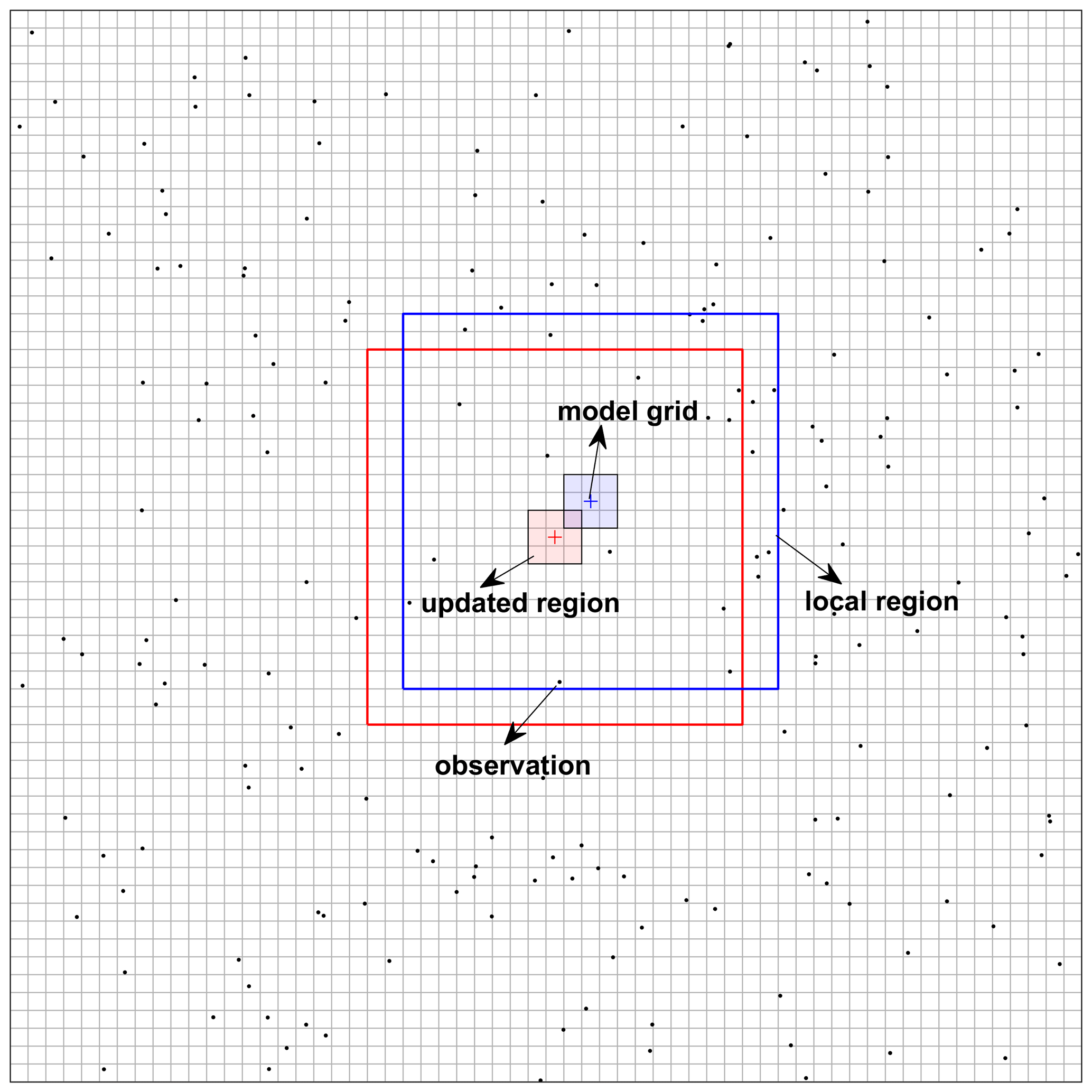
Figure 2Illustration of the local analysis scheme used in the assimilation. The plus and dot symbols denote the centres of the model grids and the location of the observation sites, respectively. The large rectangular region denotes the local region, and the shaded region denotes the updated region.
Figure 2 shows the local scheme we used in the assimilation, where the plus and dot symbols indicate the centres of the model grids and locations of the observation sites, respectively. In each model grid, only the observation sites located within a (2l+1) by (2l+1) rectangular area centred at this model grid were considered in the calculations of its analysis. The cut-off radius l was chosen as 12 model grids, approximately 180 km at a 15 km horizontal resolution. The use of a cut-off radius, however, could cause analysis discontinuities when an observation enters or leaves the local domain when moving from one model grid to another (Sakov and Bertino, 2011). To increase the smoothness of the analysis state, following Hunt et al. (2007), we artificially reduced the impact of the observations close to the boundary of the local domain by multiplying the entries in R−1 by a factor decaying from 1 to 0 with increasing distance of the observation from the central model grid. The decay factors used in this study are calculated by
where ρ(i) is the decay factor for observation i; h(i) is the distance between observation i and the central model grid point; and L is the decorrelation length, chosen as 80 km, smaller than the cut-off radius, to increase the smoothness of the analysis state. Typically, only the state of the central model grid is updated and used to construct the global analysis field. However, experience has shown that an observable discontinuity remains in the analysis over certain regions. To address this issue, following the method of Ott et al. (2004), we simultaneously updated the state of a small patch (l=1) around the central model grid (the updated region in Fig. 2) at each local analysis step. The final analysis of a given model grid was then obtained as the weighted mean of all the analysis values of this model grid. A weighted mean was necessary since the analysis of the different patches adopted different decay factors for the observation error. The weight of each analysis value in model grid i is calculated by Eq. (14):
where h(i,j) is the distance of model grid i to the central model grid of the patch generating the jth analysis value of this grid; m is the number of patches containing this model grid; and L is the decorrelation length, which was chosen as 80 km in this study.
3.1 χ2 diagnosis
We first applied the χ2 test to demonstrate the performance of our data assimilation system, which is important in evaluating the reanalysis (Miyazaki et al., 2015). The χ2 diagnosis is a robust criterion for validating the estimated background and observation error covariance in the data assimilation (e.g. Menard et al., 2000; Miyazaki et al., 2015, 2012), which is estimated by comparing the sample covariance of observation minus forecast (OmF) with the sum of estimated background and observation error covariance in the observational space (HBHT+R):
where m is the number of observations. According to the Kalman filtering theory, the mean of χ2 should approach 1 if the background and observation error covariances are properly specified, while values greater (lower) than 1 indicate the underestimation (overestimation) of the observation and/or background error covariance.
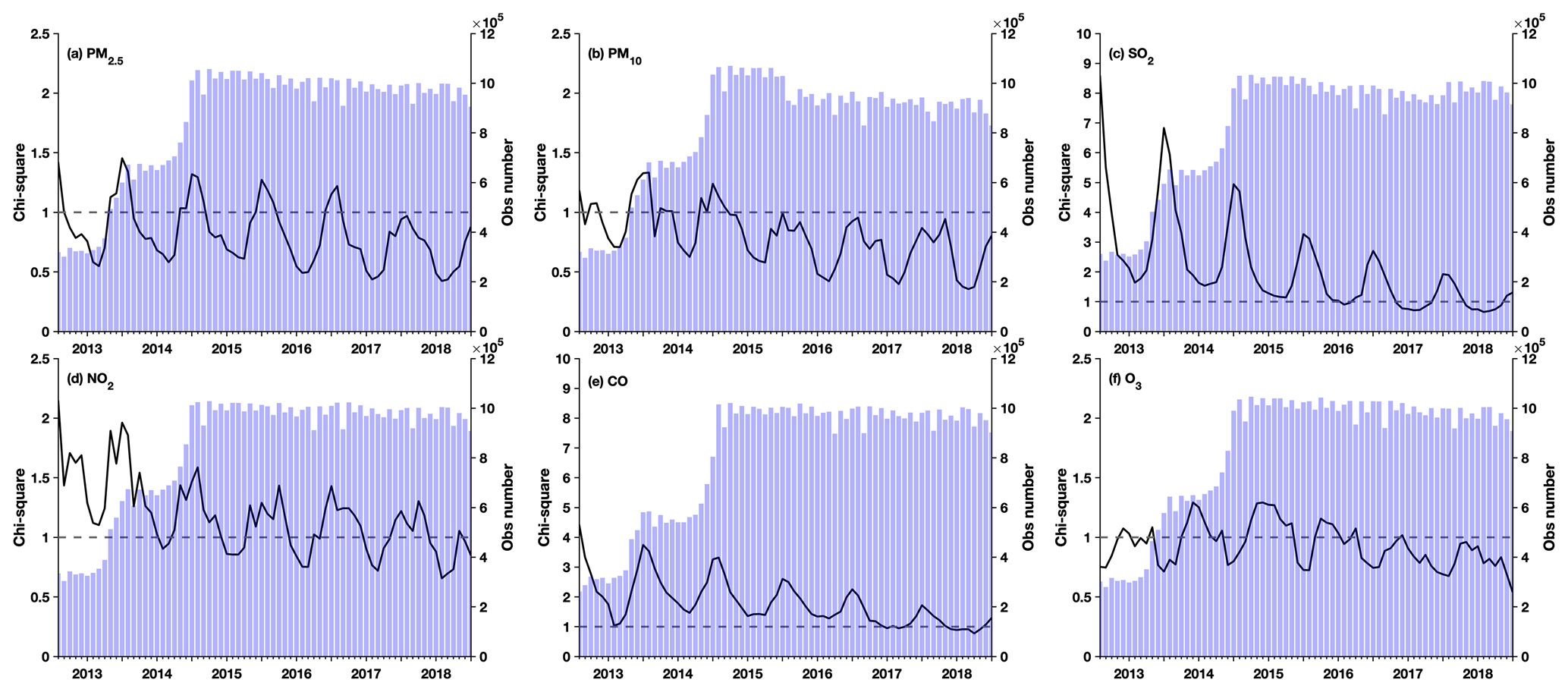
Figure 3Time series of the monthly mean χ2 values (black line) and the number of assimilated observations per month (blue bars) for (a) PM2.5, (b) PM10, (c) SO2, (d) NO2, (e) CO, and (f) O3.
Figure 3 shows the time series of the monthly χ2 values (black lines) for different species as well as the number of assimilated observations per month (blue bars). The mean values of χ2 are generally within 50 % difference from the ideal value of 1 for PM2.5, PM10, NO2, and O3, which suggests that the observation and background error covariance are generally well specified in the analysis of these species. Although the χ2 values for these species showed pronounced seasonal variations that reflect the different error characteristics in different seasons, the χ2 values were roughly stable for PM2.5 and O3 throughout the assimilation periods and for NO2 and PM10 after 2015, when the number of assimilated observations becomes stable, which generally shows the long-term stability of the performance of data assimilation. The χ2 values for SO2 were nevertheless greater than 1 in most cases, especially before 2017. This would be more relevant to the underestimations of background error covariance of SO2 as we only specified 12 % uncertainty in the SO2 emissions, suggesting that the emission uncertainty of SO2 may be underestimated by Zhang et al. (2009). There were also pronounced annual trends in the χ2 values of SO2, which may be attributed to the increase in observation number from 2013 to 2014 and the substantial decrease in SO2 observations from 2013 to 2018. Although smaller than the χ2 values of SO2, the values for CO were greater than 1 in most cases, suggesting the underestimations of the error covariances. Similar to the χ2 values of SO2, an obvious decreasing trend can also be found in the χ2 values of CO. These results suggest that our data assimilation system has relatively poor performance in the analysis of CO and SO2 concentrations compared to the other four species, which is consistent with the cross-validation results (Sect. 4.2.2), which showed smaller R2 values for the reanalysis data on CO and SO2 concentrations. The annual trend of χ2 values in CO and SO2 also indicates relatively weak stability in the performance of the data assimilation system in assimilating CO and SO2 observations, which may influence the analysis of the annual trends in these two species.
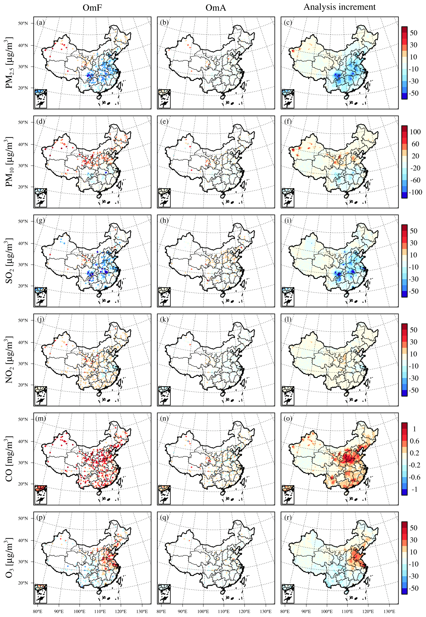
Figure 4Spatial distributions of the 6-year mean OmF (left column), OmA (middle column), and analysis increment (right column) for different species in China.
3.2 OmF & OmA analysis
Spatial distributions of 6-year average OmF and observation minus analysis (OmA) for each species in the observation space were then analysed to investigate the structure of forecast bias and to measure the improvement in the reanalysis (Fig. 4). The analysis increment, which is estimated from the differences between the analysis and forecast, is also plotted to measure the adjustments made in the model space. The OmF values showed persistent positive model biases (i.e. negative OmF) in the PM2.5 and SO2 concentrations in east China, as well as PM10 and O3 concentrations in south China. The negative model biases (i.e. positive OmF) were mainly found in the PM2.5 concentrations in west China, the PM10 concentrations in north China, the O3 concentrations in central-east China, and the concentrations of CO and NO2 throughout the whole of China.
The OmA values suggest that the data assimilation removes most of the model biases for each species, which confirms the good performance of our data assimilation system. According to Fig. C1 in Appendix C, the monthly mean OmF biases were almost completely removed in each region of China because of the assimilation, with mean OmF biases reducing by 32–94 % for PM2.5, 33–83 % for PM10, 25–96 % for SO2, 53–88 % for NO2, 88–97 % for CO, and 54–90 % for O3 concentrations in different regions of China. The mean OmF root mean square error (RMSE) was also reduced substantially by 80–93 % for PM2.5, 80–86 % for PM10, 73–96 % for SO2, 76–91 % for NO2, 88–96 % for CO, and 76–87 % for O3 concentrations in different regions of China (Fig. C2). In addition, despite the mean OmF bias and OmF RMSE exhibiting a significant annual trend, the OmA bias and OmA RMSE are relatively stable during the assimilation period, which generally confirms the long-term stability of our data assimilation system.
The spatial patterns of analysis increment were in good agreement with those of the OmF values for each species, which generally shows negative (positive) increments for PM2.5 concentrations in east (west) China, negative (positive) increments for PM10 concentrations in south (north) China, negative increments for SO2 throughout China, positive increments for CO and NO2 concentrations throughout China, and the positive (negative) increments for O3 concentrations in central-east (south) China. These results confirm that the data assimilation can effectively propagate the observation information into the model state and reduce the model errors.
In this section, we present the fields of the CAQRA dataset and compare them to the observations. It aims to provide a brief introduction to the CAQRA dataset and gives a first assessment of the quality of this dataset. The cross-validation (CV) method was applied in the assessment of the CAQRA dataset, in which a proportion of the observation data was withheld from the data assimilation process and adopted as a validation dataset. We conducted five CV experiments by randomly dividing the observation sites of the CNEMC into five groups (with 20 % of the observation sites in each group). In each experiment, the analysis was performed with one group of the observation data omitted in the assimilation process. Analysis results at the validation sites, i.e. the observation sites not used in the assimilation process, were then collected and used to validate the assimilation results. For convenience, the analysis results at the validation sites of the five CV experiments were combined and comprised a validation dataset containing all observation sites (the CV run). This dataset was then evaluated against the observations to assess the quality of the CAQRA dataset. In addition, independent PM2.5 observations retrieved from the US Department of State Air Quality Monitoring Program over China were also employed in the assessment of the PM2.5 reanalysis field. The quality of the CAQRA dataset was assessed on different spatial and temporal scales to better understand the CAQRA dataset. Additionally, the validation results of the ensemble mean of the simulations without assimilation (the base simulation) are provided to highlight the impacts of assimilation.
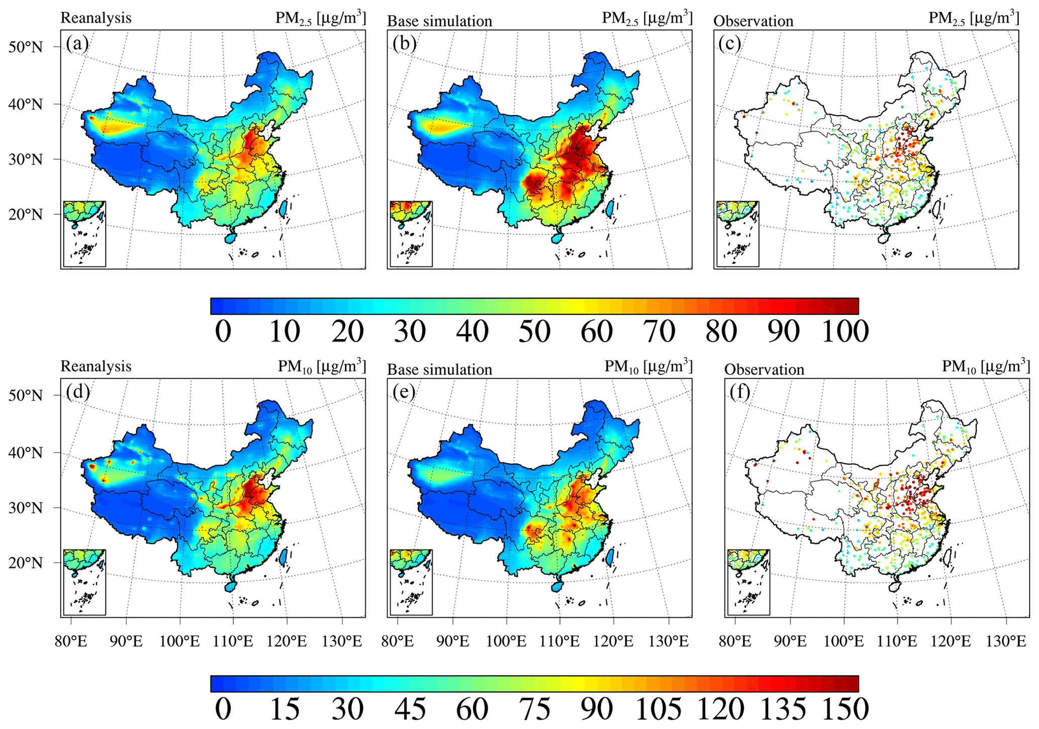
Figure 5Spatial distributions of the (a–c) PM2.5 and (d–f) PM10 concentrations in China from (a, d) CAQRA, (b, e) the base simulation, and (c, f) observations averaged from 2013 to 2018.
4.1 Particulate matter (PM)
4.1.1 Spatial distribution of the PM reanalysis data over China
We first present the reanalysis fields of the PM concentrations (PM2.5 and PM10) in China. Figure 5 shows the 6-year mean (2013–2018) spatial distribution of the PM2.5 concentration in China obtained from the CAQRA dataset, base simulation, and observations. The CAQRA dataset provides a continuous map of the PM2.5 concentration in China and suitably reproduces the observed magnitude of the PM2.5 concentration in China. The highest PM2.5 concentrations were observed in the North China Plain (NCP) region due to its intensive industrial activities and the associated high emissions of PM2.5 and its precursors (Qi et al., 2017). High PM2.5 concentrations were also found in the southeast (SE) region, where the PM2.5 concentration is influenced by both local emissions and the long-range transport of air pollutants from northern China (Lu et al., 2017). In the NW region, in addition to hotspots exhibiting high PM2.5 concentrations in large cities, high PM2.5 concentrations were observed in the Taklimakan Desert due to the influences of dust emissions. The observed magnitude and spatial variability of the PM10 concentration were also represented well by the PM10 reanalysis field. In general, the spatial distributions of the PM10 reanalysis were similar to those of the PM2.5 reanalysis except in Gansu and Ningxia provinces, where high PM10 concentrations and relatively low PM2.5 concentrations occurred. This may be related to the large contributions of dust emissions in these areas. The base simulation notably overestimated the PM2.5 and PM10 concentrations in China. This may occur due to the systematic biases in the emission inventory (Kong et al., 2020) and because negative trends of PM and its precursor emissions were not considered in our simulations. In addition, the PM2.5 concentration hotspots in the NW region and Tibetan Plateau were not captured in the base simulation, possibly due to the absence of emissions in these remote regions.
Seasonal maps of the PM2.5 and PM10 concentrations are shown in Figs. D1–D2 in Appendix D, which reveal profound seasonal variations. Both the PM2.5 and PM10 concentrations exhibit maximum values in winter in most regions of China due to the increased anthropogenic emissions related to enhanced power generation, industrial activities, and fossil fuel burning for heating purposes (M. Li et al., 2017). Unfavourable meteorological conditions with stable boundary conditions also contribute to the high PM concentrations in winter. In contrast, due to the low emission rate and intense mixing processes, the PM concentrations are the lowest in summer. The PM concentrations in the Taklimakan Desert exhibit a different seasonality, with the highest PM concentrations occurring in spring and the lowest levels occurring in winter. This occurs because the major PM sources in the Taklimakan Desert are not anthropogenic emissions but dust emissions, which are usually the highest in spring due to the frequent strong dust storms. Figure 6 further shows an example of the hourly PM reanalysis results, including a year-round time series of the site mean hourly PM concentrations in Beijing. This figure shows that PM reanalysis suitably captures the hourly evolution of the PM concentrations. Both the heavy haze episodes during the wintertime and the strong dust storms during the springtime are represented well in PM reanalysis.
Table 2Site-based cross-validation results for the reanalysis data (outside brackets) and base simulation (inside brackets) from 2013 to 2018 on the different temporal scales.
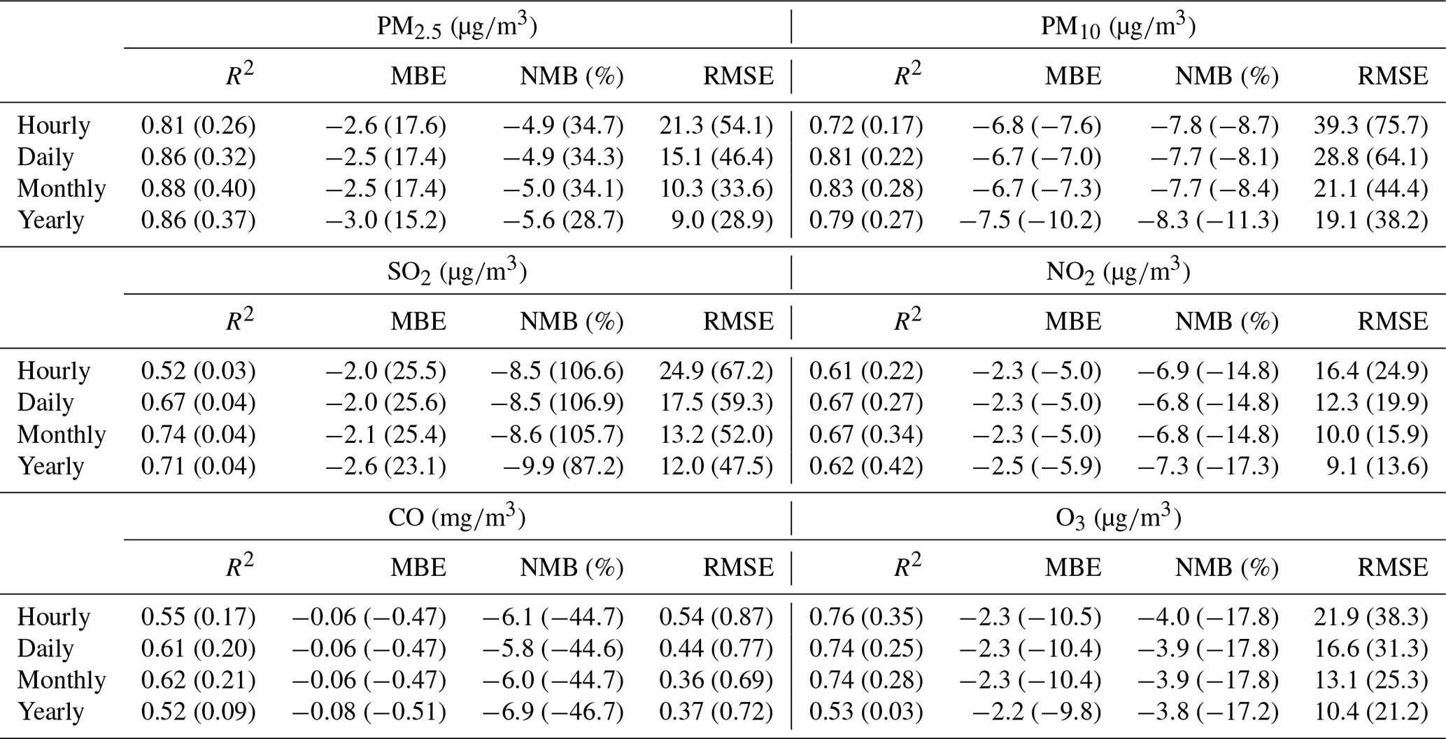

Figure 6Time series of the site mean hourly (a) PM2.5 and (b) PM10 concentrations in Beijing obtained from the observations and CAQRA.
4.1.2 Assessment of the PM reanalysis data over China
The CV method was used to assess the quality of the PM reanalysis data over China. Table 2 summarizes the site-based CV results for the reanalysis data from 2013 to 2018 on the different temporal scales. It should be mentioned that these sites are all validation sites not used in the data assimilation process. The validation results indicated that, due to assimilation of the surface PM concentrations, the reanalysis data exhibit a relatively high performance in reproducing the magnitude and variability of the surface PM concentrations in China. The CV R2 values were up to 0.81 and 0.72 in regard to the hourly PM2.5 and PM10 concentrations, respectively, which were much higher than the values of 0.26 and 0.17, respectively, in the base simulation. The bias was substantially reduced in the PM2.5 and PM10 reanalysis data, with CV mean bias error (MBE) values of approximately −2.6 (−4.9 %) and −6.8 (−7.8 %), respectively, on an hourly scale, much smaller than the large bias in the base simulation. The CV RMSE values were only approximately half of the base simulation RMSE values, which were approximately 21.3 and 39.3 for the hourly PM2.5 and PM10 concentrations, respectively. The reanalysis data showed a good performance on daily, monthly, and yearly scales, with CV RMSE values ranging from 9.0 to 15.1 for the PM2.5 concentration and from 19.1 to 28.8 for the PM10 concentration.
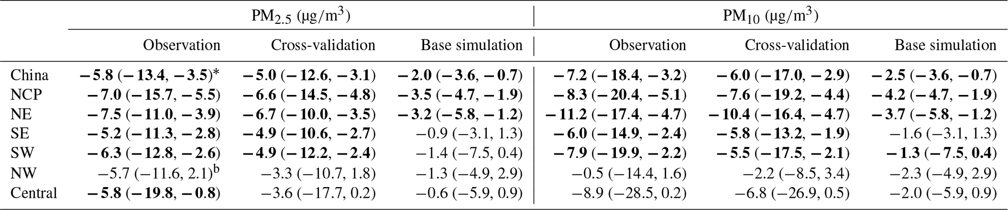
The quality of the PM2.5 and PM10 reanalysis data in the different regions of China is further summarized in Appendix E, Tables E1–E2. On an hourly scale, small negative biases of the PM2.5 reanalysis data were found in the NCP (−4.8 %), NE (−5.8 %), SE (−3.8 %), and SW (southwest, −3.4 %) regions. The biases in the NW and central regions were relatively large, with CV normalized mean bias (CV NMB) values of approximately −13.1 and −8.2 %, respectively. Two factors might explain the large biases in these two regions. First, the observation sites are sparse in the NW and central regions. As a result, the PM2.5 concentration is not suitably constrained at certain sites in the CV method. Second, the emissions of PM2.5 and its precursors might be very low in these two regions, leading to underestimation of the background errors since we only considered the emission uncertainty in the ensemble simulations. Although this problem was alleviated by using the inflation technique to compensate for the missing errors, the overconfident model results still degraded the assimilation performance to a certain extent, making the analysis less influenced by the observations. The errors of the PM2.5 reanalysis data exhibited apparent spatial differences (Table E1). The CV RMSE values were the smallest in the SE (14.9 ) and SW (16.5 ) regions and increased to ∼25 in the NCP, NE, and central regions. Consistent with the bias distributions, the largest CV RMSE value was found in the NW region, which reached 52.1 but was still much smaller than the RMSE value of the base simulation (73.0 ). The errors of the PM2.5 reanalysis data were small on daily, monthly, and yearly scales, with CV RMSE values of approximately 10.6–39.4 on a daily scale, 7.4–26.9 on a monthly scale, and 6.1–23.5 on a yearly scale. In terms of the hourly PM10 reanalysis data, the CV results (Table E2) indicated that small negative biases occurred in the NCP, NE, SE, and SW regions, ranging from −9.6 % (NE region) to −5.9 % (SE region). The biases were larger in the NW and central regions, with the CV NBM values increasing to approximately 18.0 and 14.1 %, respectively. The errors of the PM10 reanalysis data also exhibited spatial heterogeneity. The CV RMSE value was the smallest in the SE (26.0 ) and SW (30.2 ) regions and increased to approximately 39.8 and 43.7 in the NE and NCP regions, respectively. The largest errors were found in the central and NW regions, with CV RMSE values of approximately 105.5 and 57.3 , respectively. The PM10 reanalysis data revealed small errors on daily, monthly, and yearly scales, with CV RMSE values of approximately 18.6–85.5 on a daily scale, 13.7–64.0 on a monthly scale, and 12.3–55.8 on a yearly scale.
Table 3Calculated annual trends of the PM2.5 and PM10 concentrations in China.
∗ The bold font denotes that the calculated trend is significant at the 0.05 significance level, and the values in brackets denote the 95 % confidence interval.
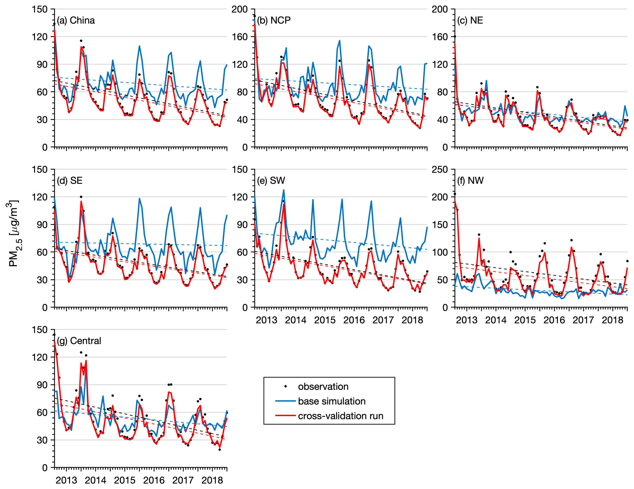
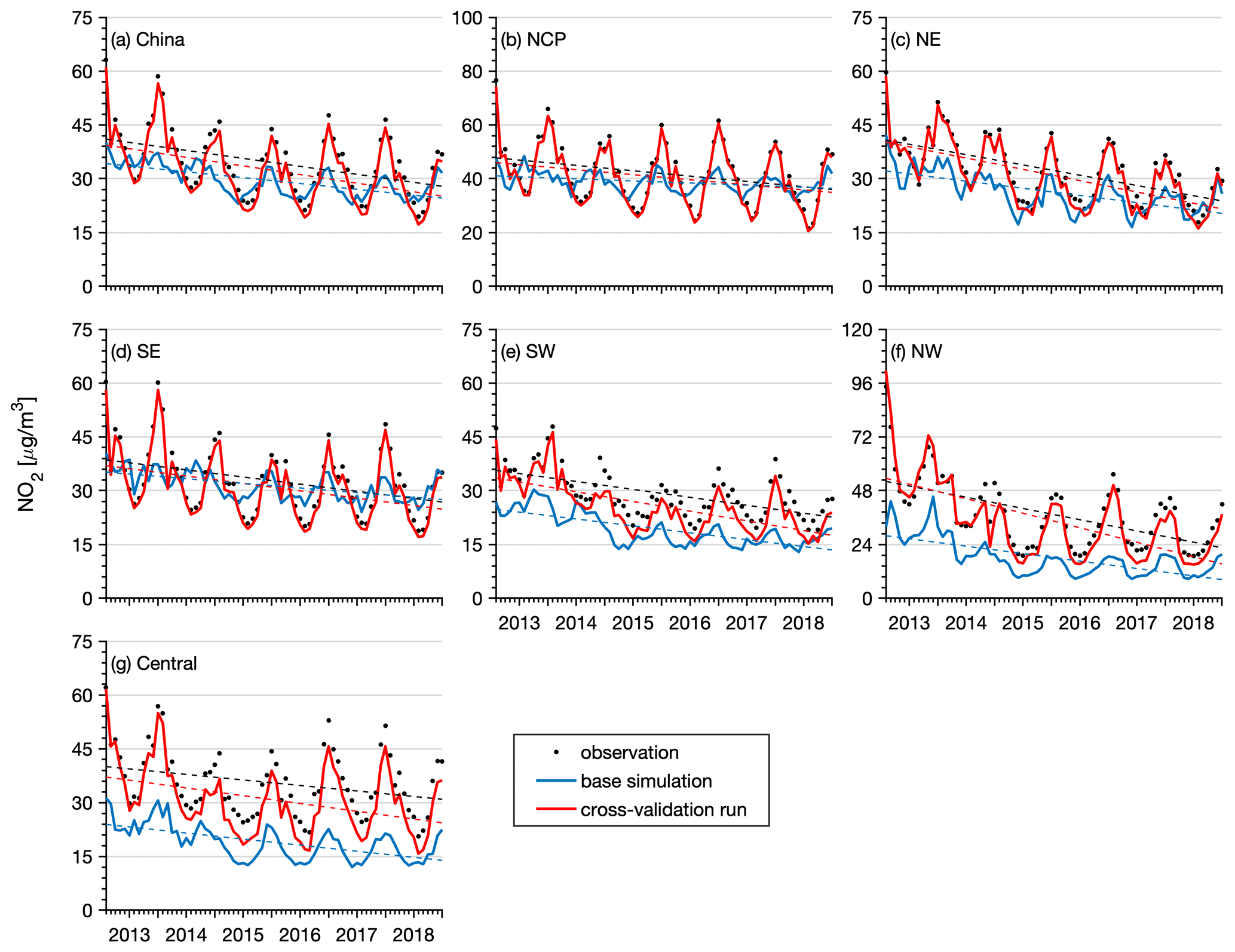
Figure 7Time series of the monthly mean PM2.5 concentrations in (a) China, (b) NCP, (c) NE, (d) SE, (e) SW, (f) NW, and (f) central regions obtained from the cross-validation run (red line), base simulation (blue line), and observations (black dots).
4.1.3 Trend study of the PM reanalysis data over China
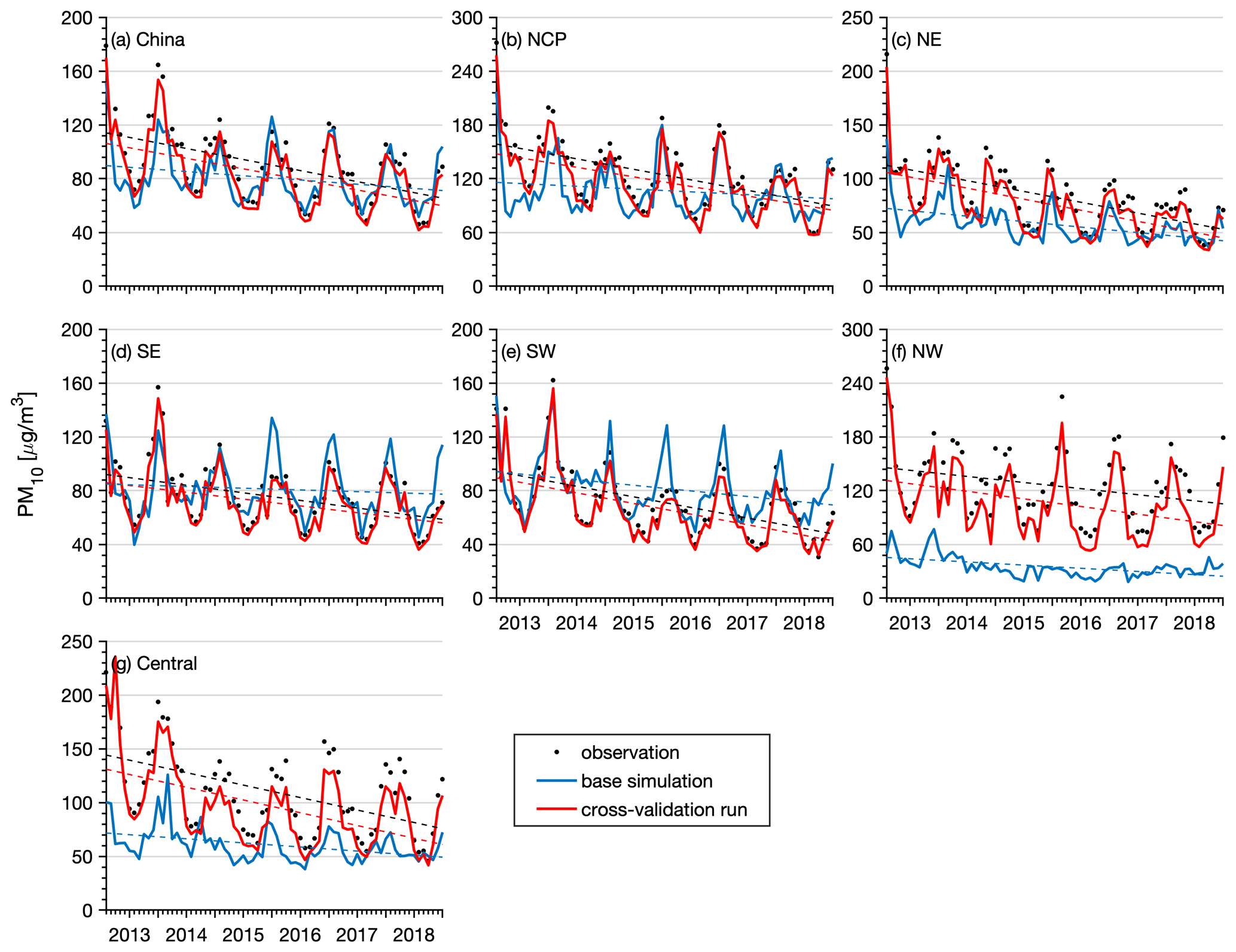
A realistic representation of the observed interannual change is another important aspect of the reanalysis dataset. The performance of the reanalysis data in representing the observed interannual changes in the PM2.5 and PM10 concentrations was thus evaluated nationwide and in the different regions of China. Figures 7–8 show time series of the monthly mean PM2.5 and PM10 concentrations nationwide and in the different regions. The observed national PM2.5 concentration revealed a profound seasonal cycle with the highest concentration in winter and the lowest level in summer. The annual trends of the PM2.5 and PM10 concentrations were also calculated using the Mann–Kendall trend test and the Theil–Sen trend estimation method, which are summarized in Table 3. A significant negative trend was observed in the PM2.5 concentration nationwide, with a calculated annual trend of approximately −5.8 (p<0.05) . The NE and NCP regions exhibited the highest negative trends among the six regions, with calculated trends of approximately −7.5 (p<0.05) and −7.0 (p<0.05) , respectively. In the other regions, the negative trends ranged from −6.3 to −5.2 . The base simulation suitably reproduced the observed seasonal cycle of the PM2.5 concentration in all regions. The magnitude of the PM2.5 concentration in 2013 was also captured well in the different regions, suggesting that the emission inventories of 2010 were generally reasonable for the simulation of the PM2.5 concentration in 2013. However, starting from 2014, the base simulation tended to overestimate the observations in the NCP, SE, and SW regions, indicating that the emission inventory of 2010 may be too high for the simulation of the PM2.5 concentration in these regions after 2014. In contrast, the base simulation significantly underestimated the PM2.5 concentration in the NW region. The model performance of the base simulation was relatively good in the NE and central regions throughout the 6 years. Although the base simulation captured the negative trends of the observed PM2.5 concentration in China and the different regions, the simulated trends were much lower than those indicated by the observations. Since we adopted the same emission inventory in the simulations of the air pollutants in the different years, the simulated trends in the base simulation were only driven by the variations in meteorological conditions. This suggests that the change in meteorological conditions only explained a small proportion of the negative trends in the PM2.5 concentration in China and that emission reductions contributed more to the decline in the PM2.5 concentration. The CV run agreed better with the observations. The observed trends of the PM2.5 concentration in China and each subregion were all suitably captured by the reanalysis in the CV run. Similar results were obtained for the analysis of the trend of the PM10 concentration, as shown in Fig. 8. The observed PM10 concentration also exhibited significant negative trends, which were captured well by the PM10 reanalysis in the CV run. The base simulation attained a better performance in reproducing the PM10 concentration in China than in reproducing the PM2.5 concentration, while significant underestimations of the PM10 concentration occurred in the NW and central regions. The calculated negative trends of the base simulation were still lower than those indicated by the observations. This again highlights the large contributions of emission reduction to the improvement of the air quality in China in these years.
Table 4Independent validation results of the CAQRA dataset (outside brackets) and base simulation (inside brackets) against the observation data retrieved from the US Department of State Air Quality Monitoring Program over China on an hourly scale.

4.1.4 Independent validation of the PM2.5 reanalysis data
In addition to the CV method, the PM2.5 reanalysis data were further validated against an independent dataset acquired from the US Department of State Air Quality Monitoring Program over China (http://www.stateair.net/; last access: 17 April 2020), which contains the hourly PM2.5 concentration in the cities of Beijing, Chengdu, Guangzhou, Shanghai, and Shenyang. Table 4 presents a comparison of the observed PM2.5 concentrations to those obtained from the CAQRA dataset and base simulation. The results indicated that the magnitude and variability of the PM2.5 reanalysis data agreed better with those of the observed PM2.5 concentrations in all cities. Both the MBE and RMSE values were greatly reduced in the CAQRA dataset, which only ranged from −7.1 to −0.3 and from 16.8 to 33.6 , respectively, in these cities. The correlation coefficient was also greatly improved in CAQRA (R2=0.74–0.86) over the base simulation (R2=0.09–0.37). These results confirm that the CAQRA dataset attains a high-quality performance in representing the PM2.5 pollution in China in these years.
Table 5Comparison of the accuracy of our PM2.5 reanalysis data to those of satellite estimates.
∗ The accuracy of the PM2.5 estimates of Lin et al. (2018) was
assessed on a monthly scale.
LME: linear mixed-effect model;
GWR: geographically weighted regression model;
GAM: generalized additive model;
HD-expansion: high-dimensional expansion;
RF: random forest;
XGBoost: extreme gradient boosting;
NELRM: non-linear exposure–lag–response model;
TEFR: time-fixed effects regression model;
GW-GBM: geographically weighted gradient boosting machine;
Geoi-DBN: geographical deep belief network.
4.1.5 Comparison to the satellite-estimated PM2.5 concentration
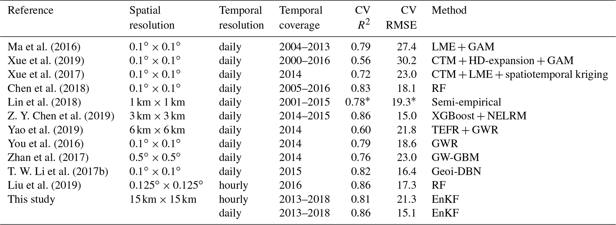
Previous studies have shown that estimating the ground-based PM2.5 concentration from the satellite-derived AOD is an effective way to map the PM2.5 concentration with good accuracy. To further demonstrate the accuracy of our PM2.5 reanalysis data, we also compared the accuracy to that of satellite-estimated PM2.5 concentrations. Table 5 summarizes several representative studies focusing on the estimation of the ground-based PM2.5 concentration in China at the national level using different kinds of methods. Most of these studies estimated the ground-based PM2.5 concentration on a daily scale since they employed polar-orbiting satellite data (e.g. MODIS) that only provide daily AOD observations. The estimation conducted by Liu et al. (2019) was an exception which exhibited an hourly resolution due to the use of AOD measurements from a geostationary satellite (Himawari-8). The horizontal resolution in these studies was mainly approximately 10 km, except that of Lin et al. (2018), which revealed the finest horizontal resolution (1 km), and that of Zhan et al., 2017, which revealed the coarsest horizontal resolution (0.5∘). Few studies have provided long-term PM2.5 data covering recent years. In comparison, our PM2.5 reanalysis data provide long-term data in China at a fine temporal resolution (1 h) and a high accuracy. A fine temporal resolution is important for epidemiological studies, especially for the assessment of the acute health effects of air pollution. Furthermore, the accuracy of our reanalysis data (CV R2=0.86 and CV RMSE =15.1 ) was also higher than that of most of these satellite estimates (CV R2=0.56–0.86 and CV RMSE =15.0–30.2 ).
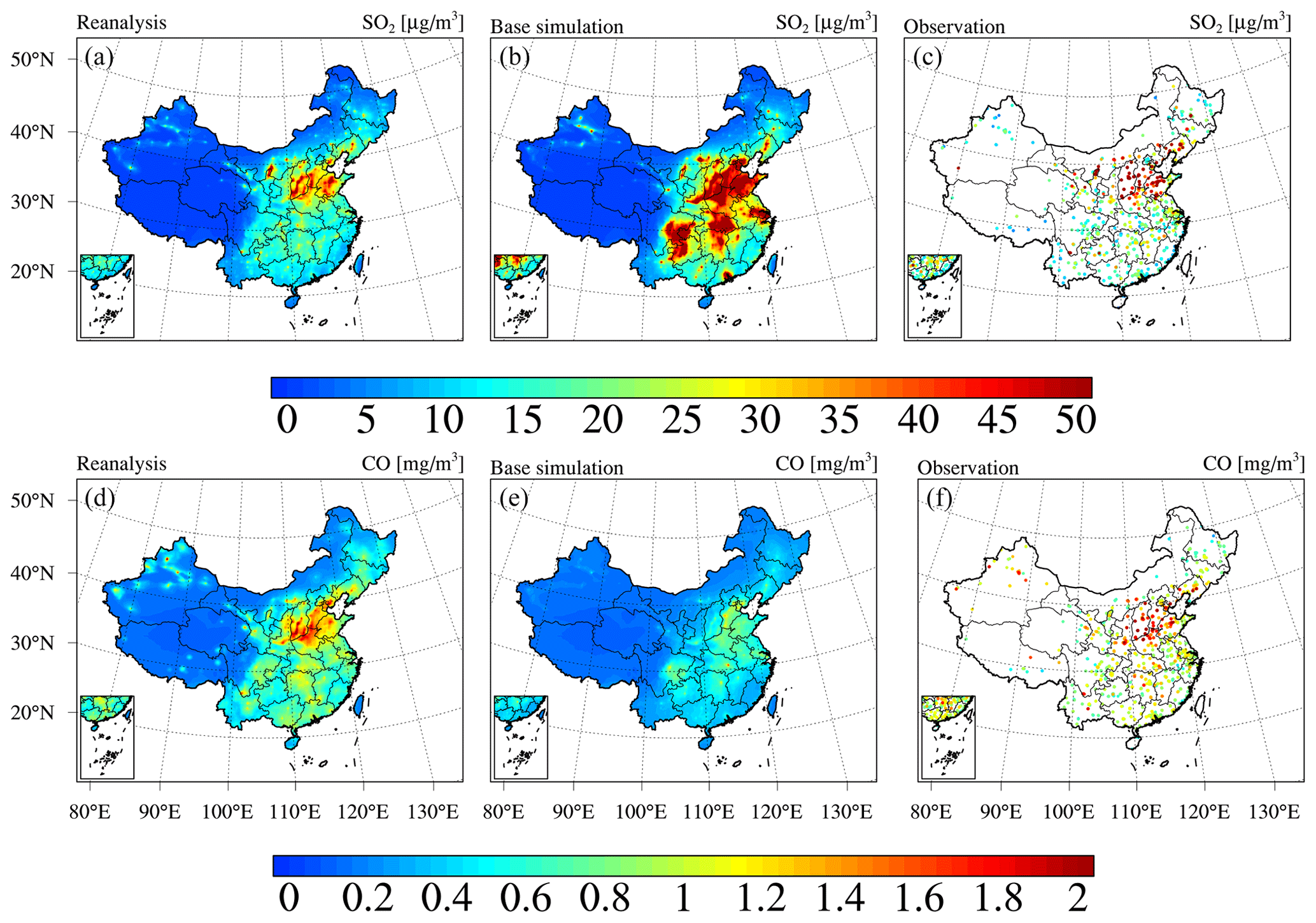
Figure 9Same as Fig. 5 but for the SO2 and CO concentrations.
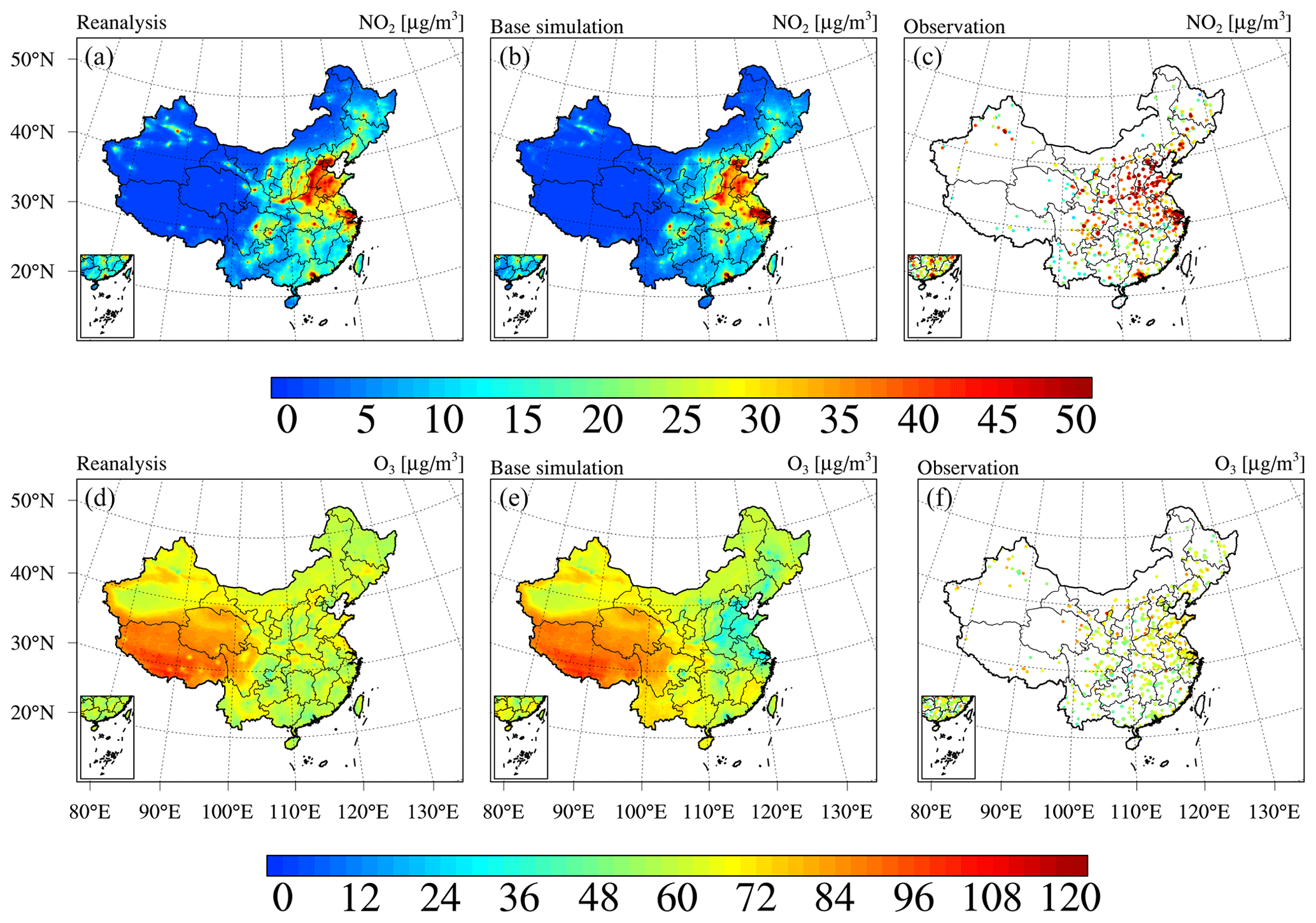
Figure 10Same as Fig. 5 but for NO2 and O3.
4.2 Gases
4.2.1 Spatial distribution of the reanalysis data on gaseous air pollutants over China
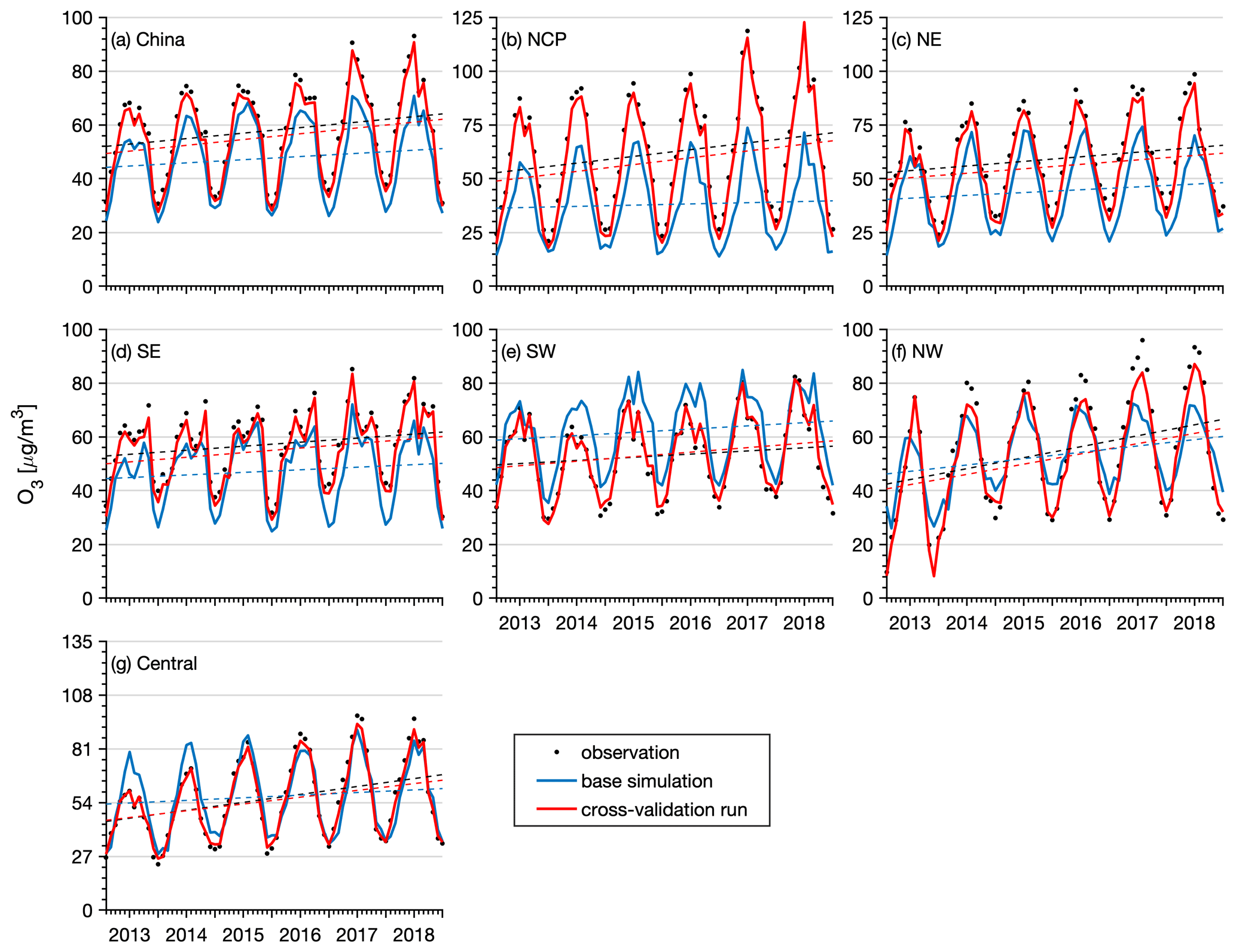
Next, we present the reanalysis fields for gaseous air pollutants in China, namely, SO2, CO, NO2, and O3. Figure 9 shows the spatial distribution of the 6-year average SO2 and CO concentrations in China obtained from the CAQRA dataset, base simulation, and observations. The SO2 reanalysis data captured the magnitude and spatial distribution of the SO2 concentration in China well, while the base simulation greatly overestimated the SO2 concentration due to the positive biases of the SO2 emissions in the simulations. Consistent with the observations, the SO2 reanalysis data exhibited high spatial heterogeneity, with the highest values located in the NCP region, especially in Shandong, Shanxi, and Hebei provinces. Several SO2 concentration hotspots were also found in the NE region. SO2 is mainly emitted from fossil fuel consumption, especially coal burning (Lu et al., 2010). Shandong, Shanxi, Inner Mongolia, and Hebei provinces are the four largest consumers of coal in China according to the China Energy Statistical Yearbook (NBSC, 2017a, b), which explains the high SO2 concentrations in these provinces. The spatial distribution of the CO reanalysis data was similar to that of the SO2 reanalysis data and agreed well with the observed spatial distribution. In contrast, the base simulation highly underestimated the CO concentration, especially in the NCP region. In addition, both the observations and reanalysis data showed CO concentration hotspots in the NW region and Xizang Province, while these hotspots were largely underestimated or even missing in the base simulation. According to previous studies, such underestimation might be related to underestimated CO emissions in China (Kong et al., 2020; Tang et al., 2013). In regard to NO2 (Fig. 10), both the reanalysis data and base simulation captured the observed magnitude and spatial distribution of the NO2 concentration in China. High NO2 concentrations generally occurred in the NCP region and the major city clusters in China. However, the base simulation generally revealed an underestimated NO2 concentration in China. The spatial distribution of the O3 concentration (Fig. 10) demonstrated a lower spatial heterogeneity than that of the other gases. The O3 reanalysis data suitably captured the observed magnitude and spatial distribution of the O3 concentration in China, while the base simulation generally underestimated the O3 concentration in China. Figures D3–D6 in Appendix D further show seasonal maps of the reanalysis fields of these gases. All gases exhibited a profound seasonal cycle, with maximum values observed in winter and the lowest values in summer, except O3, which demonstrated the opposite seasonal cycle. The highest SO2, CO, and NO2 concentrations in winter could occur due to the increased anthropogenic emissions and the more stable atmospheric conditions during this season. Regarding O3, the highest value in summer was closely related to the enhanced photochemical reactions in summer associated with the high temperature and solar radiance.
4.2.2 Assessment of the gas reanalysis data over China
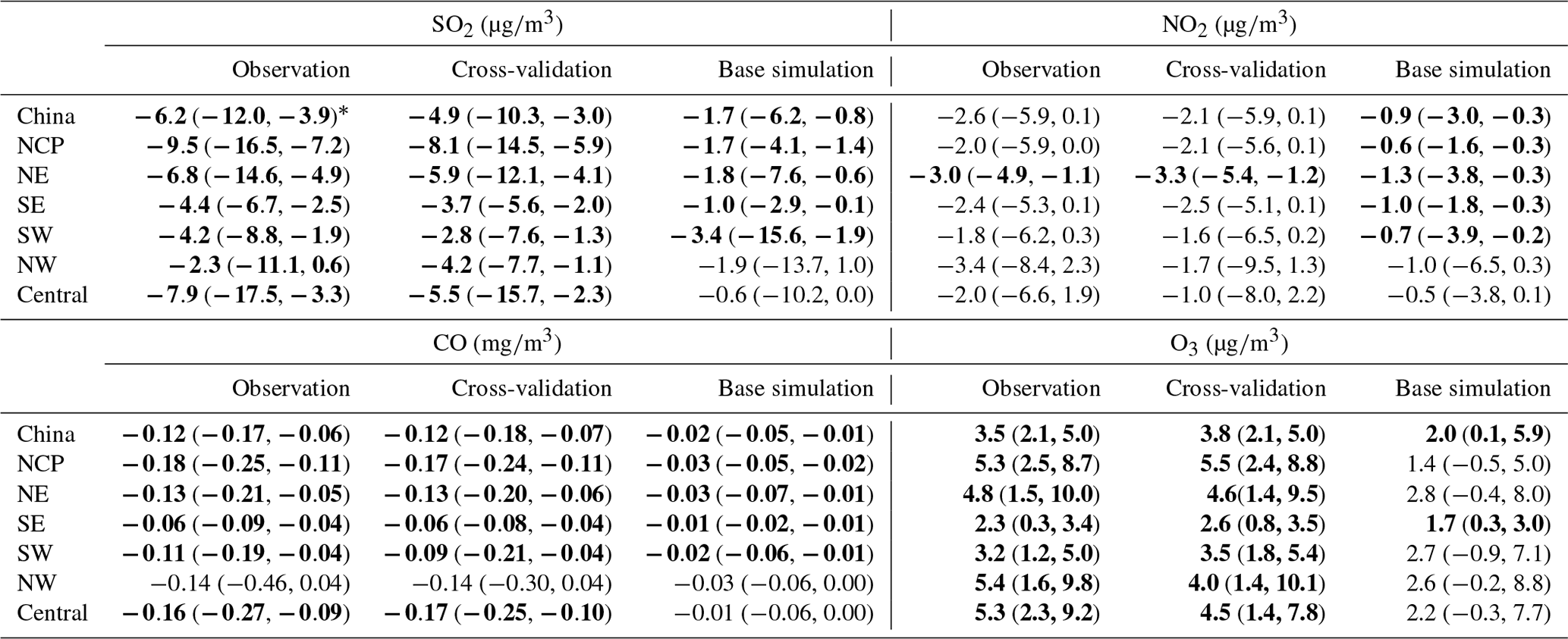
Evaluation results of the above gas reanalysis data are provided in Table 2. The table indicates that the reanalysis data attain an excellent performance in representing the magnitude and variability of these gaseous air pollutants in China, with CV R2 values ranging from 0.52 for SO2 to 0.76 for O3 and CV MBE (CV NMB) values of approximately −2.0 (−8.5 %), −2.3 (−6.9 %), −0.06 (−6.1 %), and −2.3 (−4.0 %) for the hourly SO2, NO2, CO, and O3 reanalysis data, respectively. Compared to the base simulation, the errors were reduced by approximately half in the reanalysis data, with CV RMSE values of approximately 24.9 , 16.4 , 0.54 , and 21.9 for the hourly SO2, NO2, CO, and O3 reanalysis data, respectively. The reanalysis data achieved a good performance on daily, monthly, and yearly scales. The CV RMSE values of the daily SO2 and NO2 reanalysis data were also smaller than those of the SO2 and NO2 concentration datasets in China previously developed by Zhan et al. (2018) and Zhang et al. (2019), respectively, based on the random forest–spatiotemporal kriging model wherein the RMSE values of the daily SO2 and NO2 concentrations were estimated to be 19.5 and 13.3 , respectively.
In terms of the different regions (Tables E3–E6, Appendix E), the hourly SO2 reanalysis data indicated small negative biases (approximately 2–10 %) in all regions except the central region, where the negative bias was relatively large (17.0 %). The smallest CV RMSE values of the SO2 reanalysis data were observed in the SE, SW, and NW regions (smaller than 25 ), while in the other regions the CV RMSE values exceeded 30 . The hourly NO2 reanalysis data showed small negative biases in all regions, which were relatively small in the NE, NCP, and SE regions (ranging from −5.9 to −3.5 %) and were relatively large in the SW, NW, and central regions (ranging from −15.1 to −12.9 %). The CV RMSE for the hourly NO2 reanalysis data was approximately 15 in all regions except the NW (24.3 ) and central (20.5 ) regions. The hourly CO reanalysis data exhibited small negative biases in all regions. The largest biases were still found in the NW region, which reached approximately 15.0 %, while in the other regions the biases ranged from −11.2 to −2.5 %. The CV RMSE values for the hourly CO reanalysis data were the smallest in south China (approximately 0.39 and 0.46 in the SE and SW regions, respectively) and increased to 0.64 and 0.59 in the NCP and NE regions, respectively. The largest CV RMSE was observed in the NW region, which amounted to approximately 1.13 . The biases of the hourly O3 reanalysis data were uniformly distributed in the different regions, with the CV NMB value ranging from −6.1 to 1.4 %. Similarly, the CV RMSE value of the O3 reanalysis data was approximately 20 in all regions except the NW region (28.3 ).
Table 6Calculated annual trends of the SO2, NO2, CO, and O3 concentrations in China.
∗ The bold font denotes that the calculated trend is significant at the 0.05 significance level, and the values in brackets denote the 95 % confidence interval.
4.2.3 Trend study of the gas reanalysis data over China
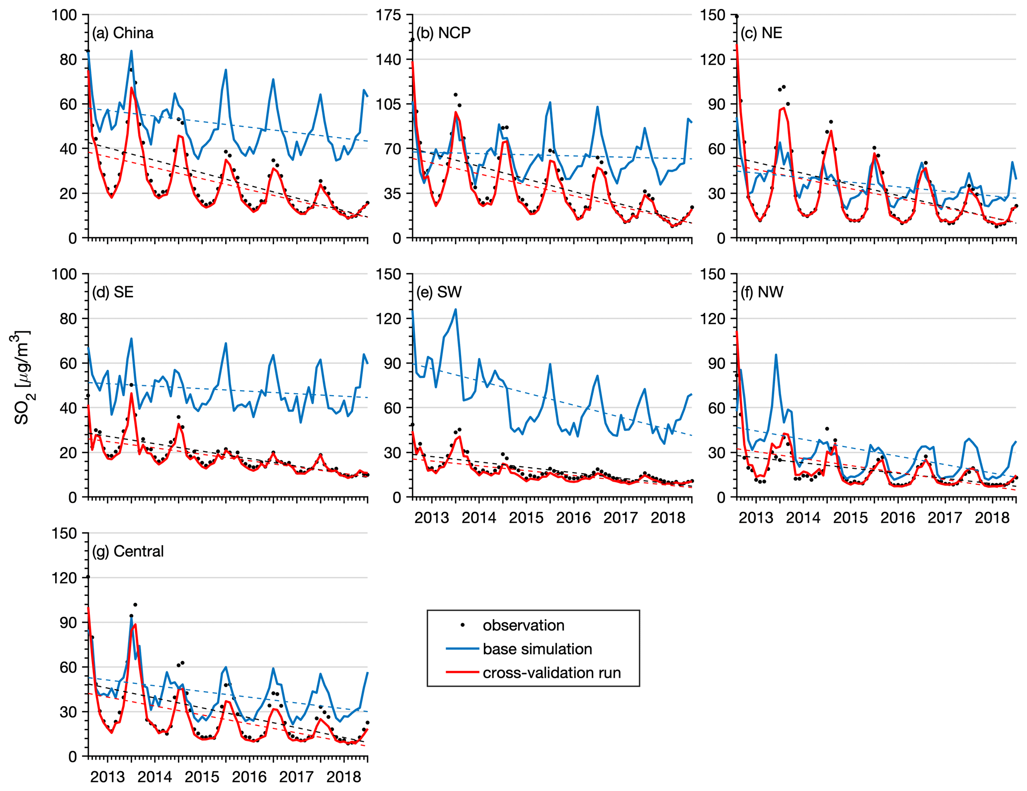
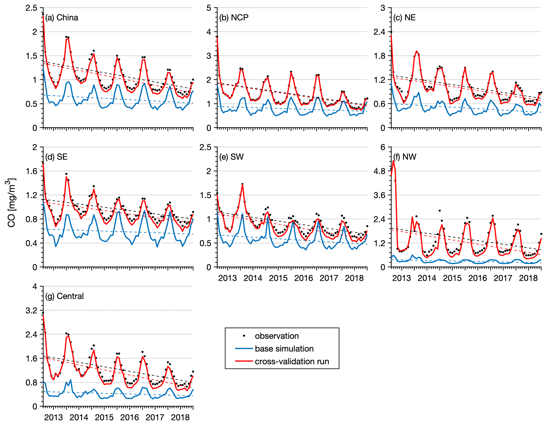
Figure 11 shows time series of the monthly mean SO2 concentration in China obtained from the CV run, base simulation, and observations. Additionally, time series of the monthly mean SO2 concentration in the different regions are shown. The observed SO2 concentrations showed significant negative trends (P<0.05) in China (−6.2 , Table 6) and in all regions (ranging from −2.3 to −9.5 , Table 6) due to the large reductions in SO2 emissions across China. During the 11th–13th Five-Year Plans (FYPs) and the Air Pollution Prevention and Control Plan, the Chinese government invested great effort to reduce SO2 emissions, such as the installation of flue-gas desulfurization (FGD) and selective catalytic reduction systems, construction of large units, decommissioning of small units, and replacement of coal with cleaner energies (M. Li et al., 2017; Zheng et al., 2018b). As a result, the SO2 emissions substantially decreased in China, especially in the industrial and power sectors. The base simulation significantly overestimated the SO2 concentration in all regions, especially after 2013. The negative trends of the SO2 concentration were also largely underestimated in the base simulation. In contrast, the SO2 reanalysis data captured the magnitude and negative trends of the observed SO2 concentrations in China and in all regions well. The NO2 observations showed negative trends in China as well (Fig. 12). However, the negative trend was not significant except in the NE region (Table 6). This is consistent with the small reductions in NOx emissions (21 %) in China due to the small changes in the emissions originating from the transportation sector, accounting for almost one-third of the NOx emissions in China. The pollution controls applied in the transportation section were exactly offset by the growing emissions related to vehicle growth (Zheng et al., 2018b). The base simulation generally underestimated the NO2 concentration during the wintertime, and the observed negative trends of the NO2 concentration were also underestimated in all regions. Due to assimilation of the observed NO2 concentrations, the reanalysis data agreed better with the observations in regard to both the magnitude and negative trends. The CO observations exhibited significant negative trends in all regions except the NW region (Fig. 13), with calculated negative trends ranging from −0.18 to −0.06 . Such negative trends have also been observed in satellite measurements, such as MOPITT observations (Zheng et al., 2018a), which are mainly attributed to the reduced anthropogenic emissions in China, as suggested by both bottom-up and top-down methods (Zheng et al., 2019). The base simulation largely underestimated the CO concentration in all regions. In addition, the negative trends of the CO concentration were also notably underestimated in the base simulation, which highlights the major contribution of emission reduction to the decreased CO concentration in these regions. The CO reanalysis data agreed well with the observations and captured the negative trends of the CO concentration in all regions. The O3 concentration exhibited the opposite trend to that exhibited by the other air pollutants (Fig. 14), which revealed significant positive trends in all regions, ranging from 2.3 to 5.4 and indicating enhanced photochemical pollution in China. This phenomenon has been observed and investigated by K. Li et al. (2019), who suggested that the rapid decrease in the PM2.5 concentration and the resultant reduction in the aerosol sink of hydroperoxyl (HO2) radicals were important factors contributing to the enhanced O3 concentration in China. The base simulation generally captured the magnitude of the O3 concentration in the SE, SW, NW, and central regions but underestimated the O3 concentration in the NCP and NE regions, especially in spring and summer. In addition, the base simulation underestimated the observed positive trends of the O3 concentration in all regions, which suggests that meteorological variability only contributed a small proportion of the observed O3 trend in China. Again, the O3 reanalysis data are substantially better than the base simulation and suitably reproduce the observed trends of the O3 concentration in all regions.
4.2.4 Comparison to the CAMS reanalysis data
To further evaluate the accuracy of our reanalysis dataset for gaseous air pollutants, the CAMSRA dataset produced by the ECMWF (Inness et al., 2019) was employed as a reference in a comparison to our reanalysis dataset. The CAMSRA dataset is the latest global reanalysis dataset on atmospheric composition, which assimilates satellite retrievals of O3, CO, NO2, and AOD. Three-hour reanalysis data on the SO2, NO2, CO, and O3 concentrations at the surface model level from 2013 to 2018 were adopted in this study, which were downloaded from https://atmosphere.copernicus.eu/copernicus-releases-new-global-reanalysis-data-set-atmospheric-composition (last access: 17 April 2020) at a resolution of 1∘ by 1∘. Here, we only focus on a comparison of the gaseous pollutants since the CAMSRA dataset does not provide PM2.5 and PM10 concentrations.
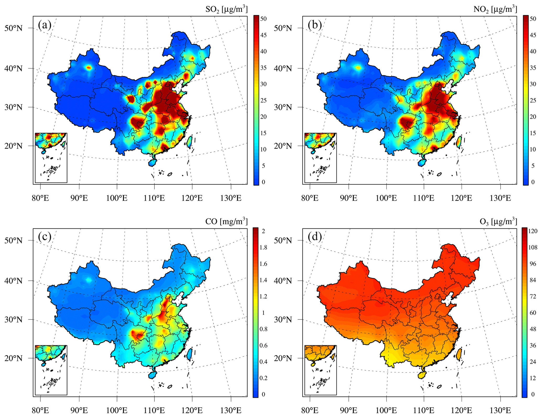
Figure 15Spatial distributions of the multiyear average concentrations of (a) SO2, (b) NO2, (c) CO, and (d) O3 from 2013 to 2018 obtained from CAMSRA.
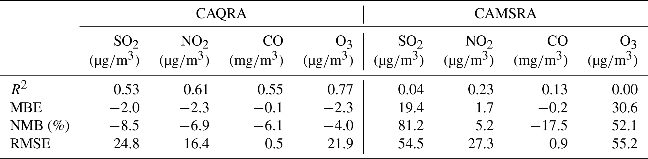
Figure 15 shows the spatial distribution of the 6-year average concentration of these gaseous air pollutants in China obtained from the CAMSRA dataset. Compared to the spatial distributions determined with the CAQRA dataset and observations (Figs. 9–10), the CAMSRA dataset greatly overestimates the surface SO2 and O3 concentrations in China. In addition, due to the higher spatial resolution (15 km) of the CAQRA dataset than that of the CAMSRA dataset (approximately 50 km), our products provide more detailed spatial patterns of the surface air pollutants in China, which are better suited for air quality studies on a regional scale. Table 7 quantitatively compares the accuracy of the CAQRA dataset to that of the CAMSRA dataset in the estimation of the surface concentrations of gaseous air pollutants in China. Compared to CAMSRA (R2=0.00–0.23), CAQRA attains a better performance in capturing the spatiotemporal variability in the surface concentrations of gaseous air pollutants in China, with R2 values ranging from 0.53 to 0.77. The MBE and RMSE values are also smaller in the CAQRA dataset than those in the CAMSRA dataset, especially for the SO2 and O3 concentrations. This is attributed to the assimilation of surface observations in CAQRA, while CAMSRA only assimilates satellite retrievals. These results suggest that the CAQRA dataset provides surface air quality datasets in China of a higher quality than the air quality datasets provided by the CAMSRA dataset, which is especially valuable for relevant future studies with high demands on spatiotemporal resolution and accuracy.
Table 7Comparison of the data accuracy of CAQRA and CAMSRA in China on an hourly scale.
The CAQRA dataset can be freely downloaded at https://doi.org/10.11922/sciencedb.00053 (Tang et al., 2020a), and the prototype product, which contains the monthly and annual means of the CAQRA dataset, is available at https://doi.org/10.11922/sciencedb.00092 (Tang et al., 2020b). When you click the first Science DB link, you will see basic descriptions of the CAQRA dataset and 2192 zip files listed in the DATA FILES column on the website. The total file sizes are approximately 318.81 GB as of the time of this writing. Each zip file is named by the date and contains one day's reanalysis data, which are composed of 24 Network Common Data Form (NetCDF) files. Each NetCDF file contains one hour's reanalysis data and is named by the date. The time zone of the reanalysis data is Beijing Time, and the description on the content of each NetCDF file is available in README.txt on the website. The monthly and annual versions of the CAQRA dataset each contain a zip file, corresponding to the monthly and annual mean of the reanalysis data, respectively. The total file sizes of this product are approximately 480.67 MB, which is easier to downloaded and suitable for users who only need air quality data on monthly or yearly scales.
A high-resolution CAQRA dataset was produced in this study by assimilating surface observations of the PM2.5, PM10, SO2, NO2, CO, and O3 concentrations retrieved from the CNEMC. This dataset provides time-consistent concentration fields of PM2.5, PM10, SO2, NO2, CO, and O3 in China from 2013 to 2018 (will be extended in the future on a yearly basis) at high spatial (15 km) and temporal (1 h) resolutions. The CAQRA dataset was produced with the ChemDAS, which applied the NAQPMS model as the forecast model, and the LETKF to assimilate the observations in the postprocessing mode. The background error covariance was calculated from ensemble simulations, which considered the emission uncertainties of the major air pollutants. An inflation technique was also applied to dynamically inflate the background error to prevent underestimation of the true background error covariance.
The 5-fold CV method was employed to validate the reanalysis dataset, which provided us with the first indication of the quality of the CAQRA dataset. The validation results suggested that the CAQRA dataset attains an excellent performance in representing the spatiotemporal variability of surface air pollutants in China, with CV R2 values ranging from 0.52 for the hourly SO2 concentration to 0.81 for the hourly PM2.5 concentration. The CV MBE values of the reanalysis data were −2.6 , −6.8 , −2.0 , −2.3 , −0.06 , and −2.3 for the hourly concentrations of PM2.5, PM10, SO2, NO2, CO, and O3, respectively. The CV RMSE values of the reanalysis data for these air pollutants were estimated to be approximately 21.3 , 39.3 , 24.9 , 16.4 , 0.54 , and 21.9 , respectively. In the different regions of China, the NW and central regions exhibited relatively large biases and errors, which mainly occurred due to the relatively sparse observations and underestimated background errors. Chinese air quality has substantially changed over the last 6 years. The observations indicate significant decreasing trends for all air pollutants except O3, which shows an increasing trend over the last 6 years. The reanalysis data reveal an excellent performance in representing the trends of all air pollutants in China, suggesting the suitability of the reanalysis data for air pollutant trend analysis in China.
In addition to the CV method, the PM2.5 reanalysis data were also evaluated against independent observations retrieved from the US Department of State Air Quality Monitoring Program over China. The results suggested that the reanalysis data suitably reproduce the magnitude and variability of the observed PM2.5 concentration in all cities, with the MBE and RMSE values only ranging from −7.1 to −0.3 and from 16.8 to 33.6 , respectively. The reanalysis data on the gaseous air pollutants were also compared to the latest global reanalysis data contained in the CAMSRA dataset produced by the ECMWF. The CAMSRA dataset is of great value in providing three-dimensional distributions of multiple chemical species globally. As a regional dataset, our products attain a higher spatial resolution than does the CAMSRA dataset, which could better suit air quality studies on a regional scale. Although our products only provide the surface concentrations of six conventional air pollutants in China, the accuracy of the CAQRA dataset was estimated to be higher than that of the CAMSRA dataset due to the assimilation of surface observations. Hence, our products exhibit their own value in regional air quality studies with high demands on spatiotemporal resolution and accuracy. We also compared our PM2.5 reanalysis data to previous satellite estimates of the surface PM2.5 concentration, which revealed that the PM2.5 reanalysis data are more accurate than most satellite estimates and exhibit a relatively fine temporal resolution.
As the first version of the CAQRA dataset, certain limitations remain that potential users should be aware of. Firstly, the discontinuities in the availability and coverage of assimilated observations will affect the reanalysis quality and the estimated interannual trends. As shown in Sect. 3.1, there has been a consistent increase in the number of assimilated observations from 2013 to 2015 due to the increases of observation sites. The smaller number of assimilated observations in 2013 and 2014 would provide fewer constraints on the background state and thus degrade the reanalysis in these 2 years. This may cause spurious interannual changes and trends from 2013 to 2018. Thus, caution is needed when using the reanalysis for long-term air quality change from 2013 to 2018. However, this problem would be not serious after 2015, when the number of assimilated observations becomes stable. In addition, the observation sites used in the assimilation are mainly urban or suburban sites that do not provide enough information on the air pollution in rural areas, which may influence the quality of CAQRA in rural areas. Secondly, we only perturbed the emissions to represent the forecast uncertainty in this study, which may underestimate the forecast uncertainty due to the omitting of other error sources, such as the uncertainty in poorly parameterized physical or chemical processes, and the uncertainty in meteorological simulation. The limited ensemble size would also lead to underestimation of the forecast error, especially in the high-resolution assimilation applications. Although the inflation method is used to compensate for the missing errors, the underestimated forecast uncertainty would still degrade the assimilation performance to a certain extent as exemplified by the larger biases in the reanalysis over the NW and central regions. Thirdly, we did not consider the annual trend of emissions in the ensemble simulation. This would lead to temporal changes in the statistics of innovation due to the substantial changes of observations, which would influence the long stability of the data assimilation as suggested by the χ2 test, although the OmA statistics generally confirm a passable stability in our assimilation system. Last but not least, the current CAQRA only contains the surface concentrations of the air pollutants in China, which cannot provide the information on the vertical structure of the air pollutants. To further improve the accuracy of our air quality reanalysis dataset, in the future, an online EnKF run could be conducted to simultaneously correct the emissions and concentrations. More observation types, such as observation data on PM2.5 composition, could also be assimilated to provide PM2.5 composition fields in China, which could support both epidemiological studies and climate research.
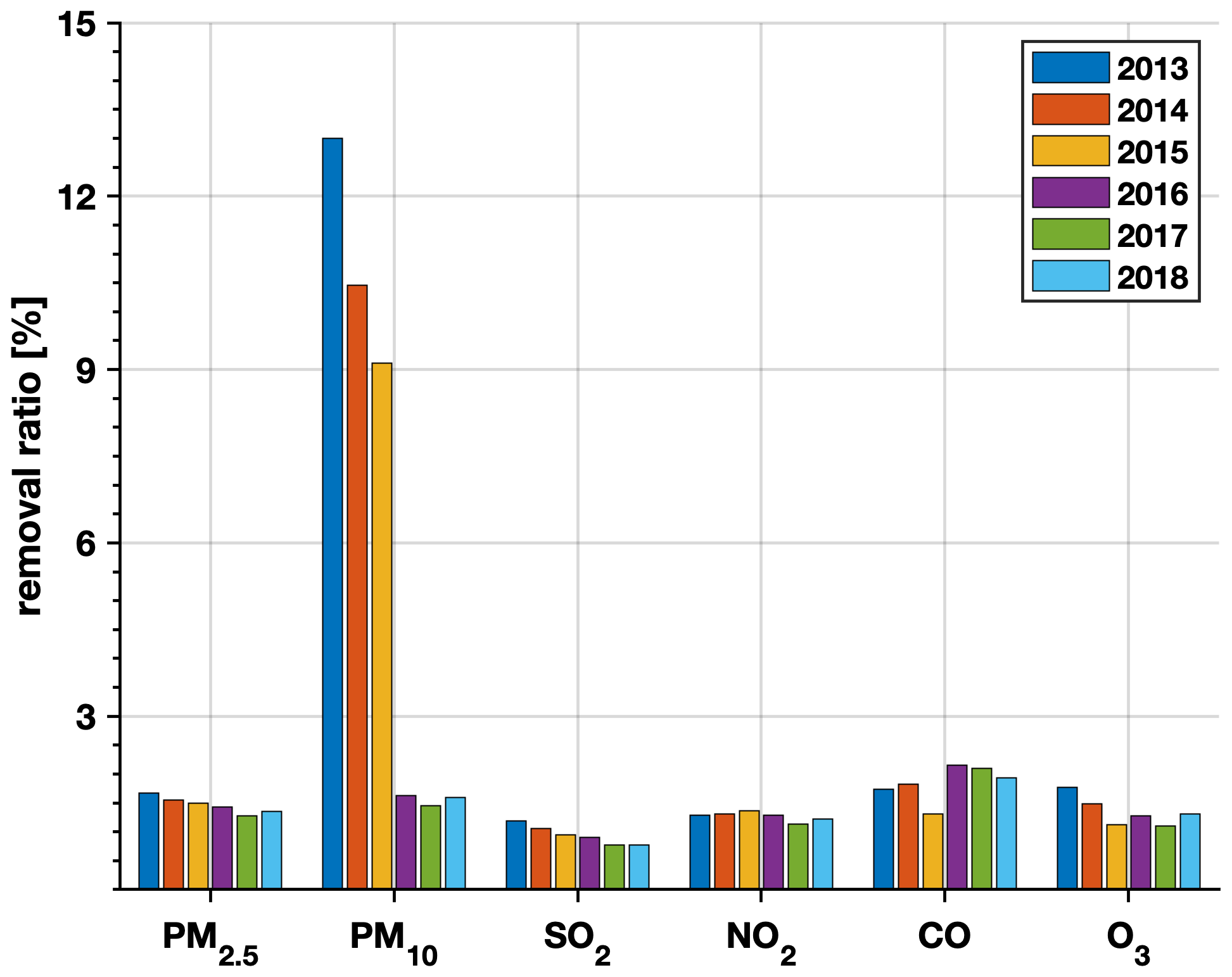
Figure A1Removal ratio of the observations in China from 2013 to 2018 for different species detected by the automatic outlier detection method.

Figure A2Spatial distributions of differences in annual concentrations of six air pollutants in China before and after quality control averaged from 2013 to 2018.
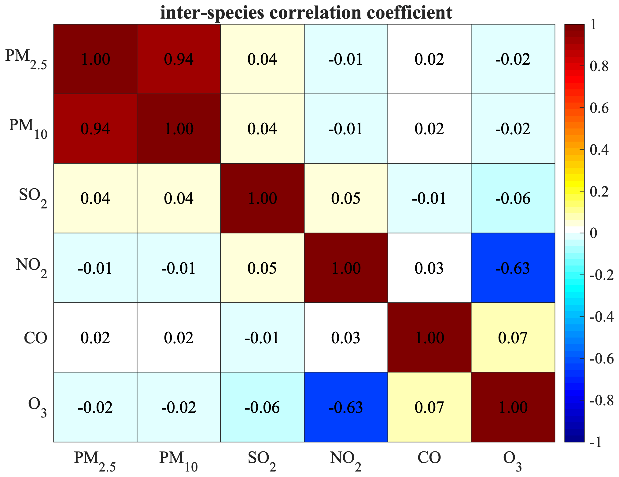
Figure B1Correlations between species in the background error covariance matrix, estimated from the LETKF ensemble averaged from 2013 to 2018. The global mean of the covariance estimated for each station is plotted.
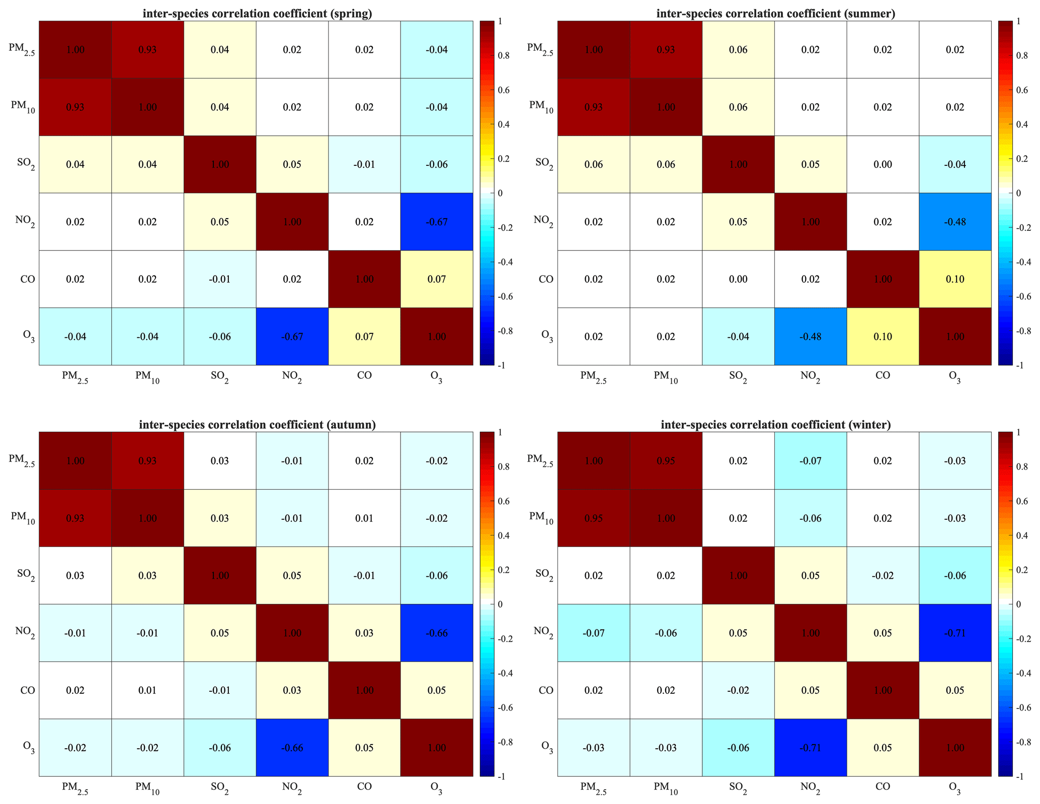
Figure B2Correlations between species in the background error covariance matrix, estimated from the LETKF ensemble averaged in different seasons from 2013 to 2018. The global mean of the covariance estimated for each station is plotted.

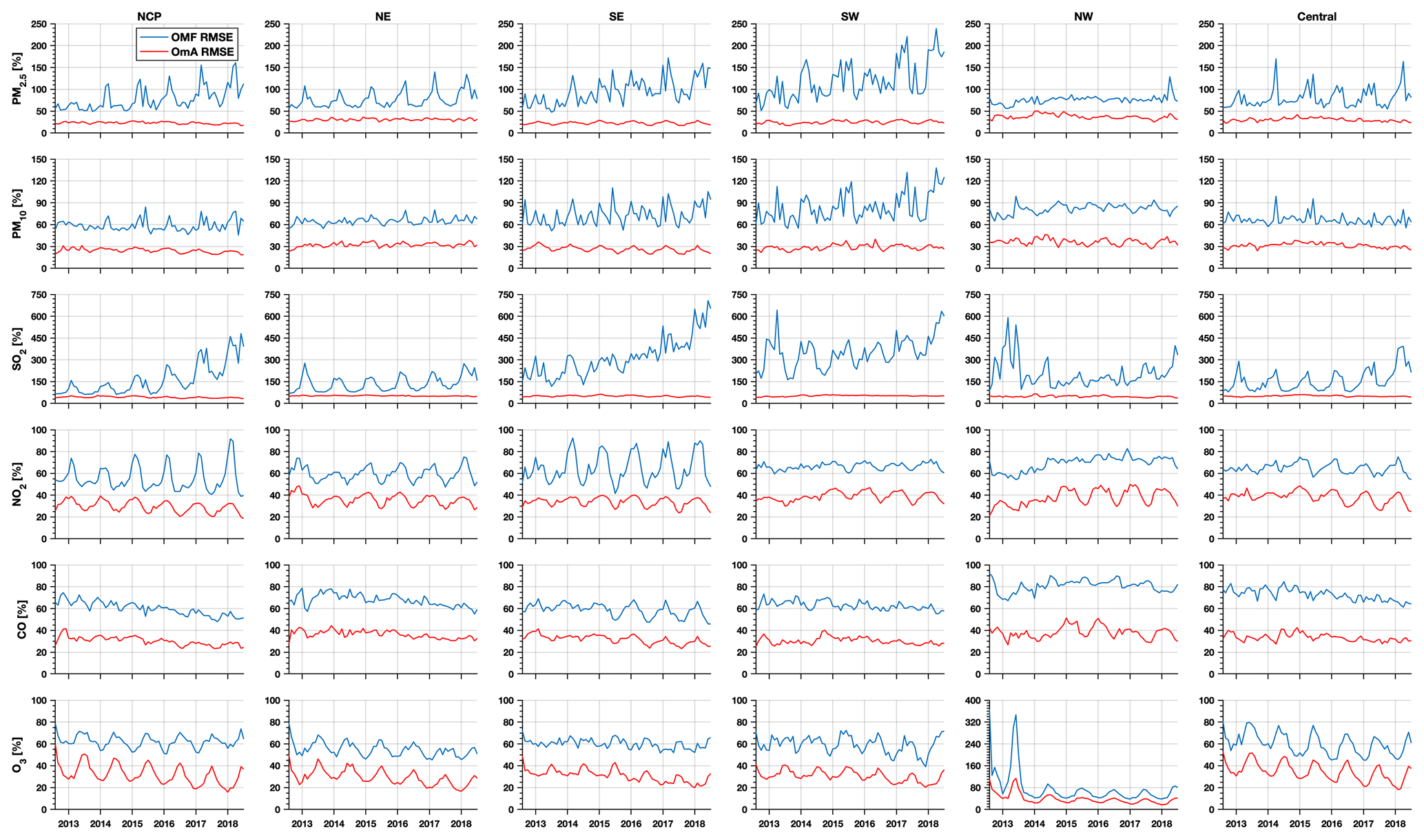
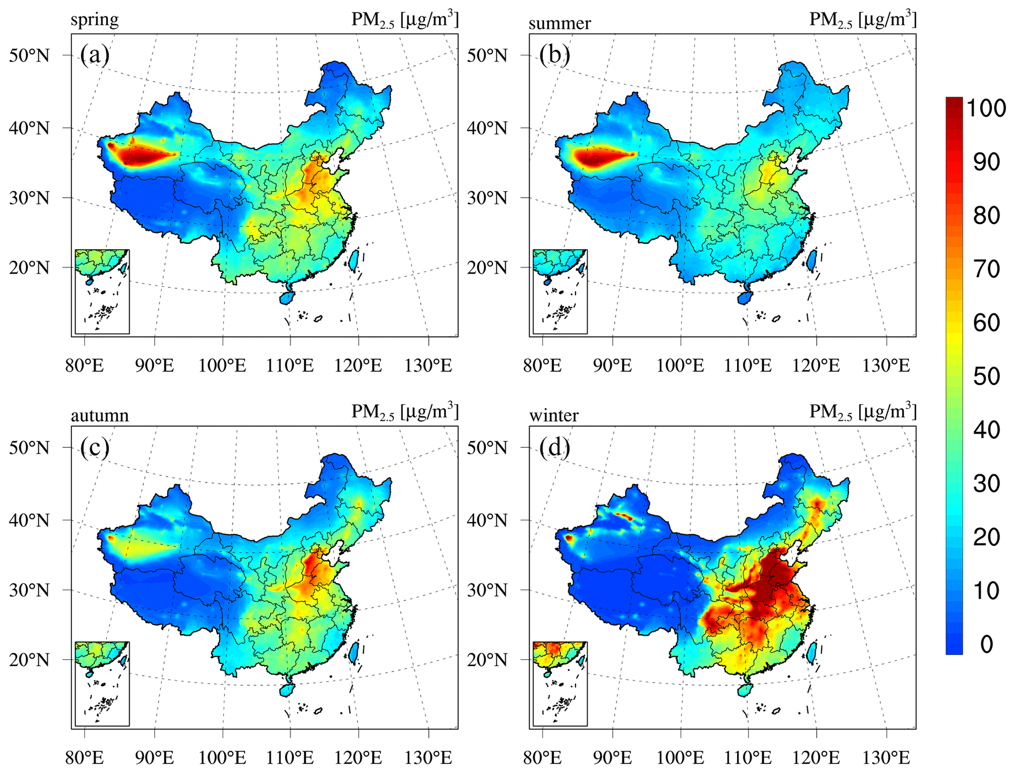
Figure D1Spatial distributions of the PM2.5 reanalysis in China during (a) spring, (b) summer, (c) autumn, and (d) winter averaged from 2013 to 2018.
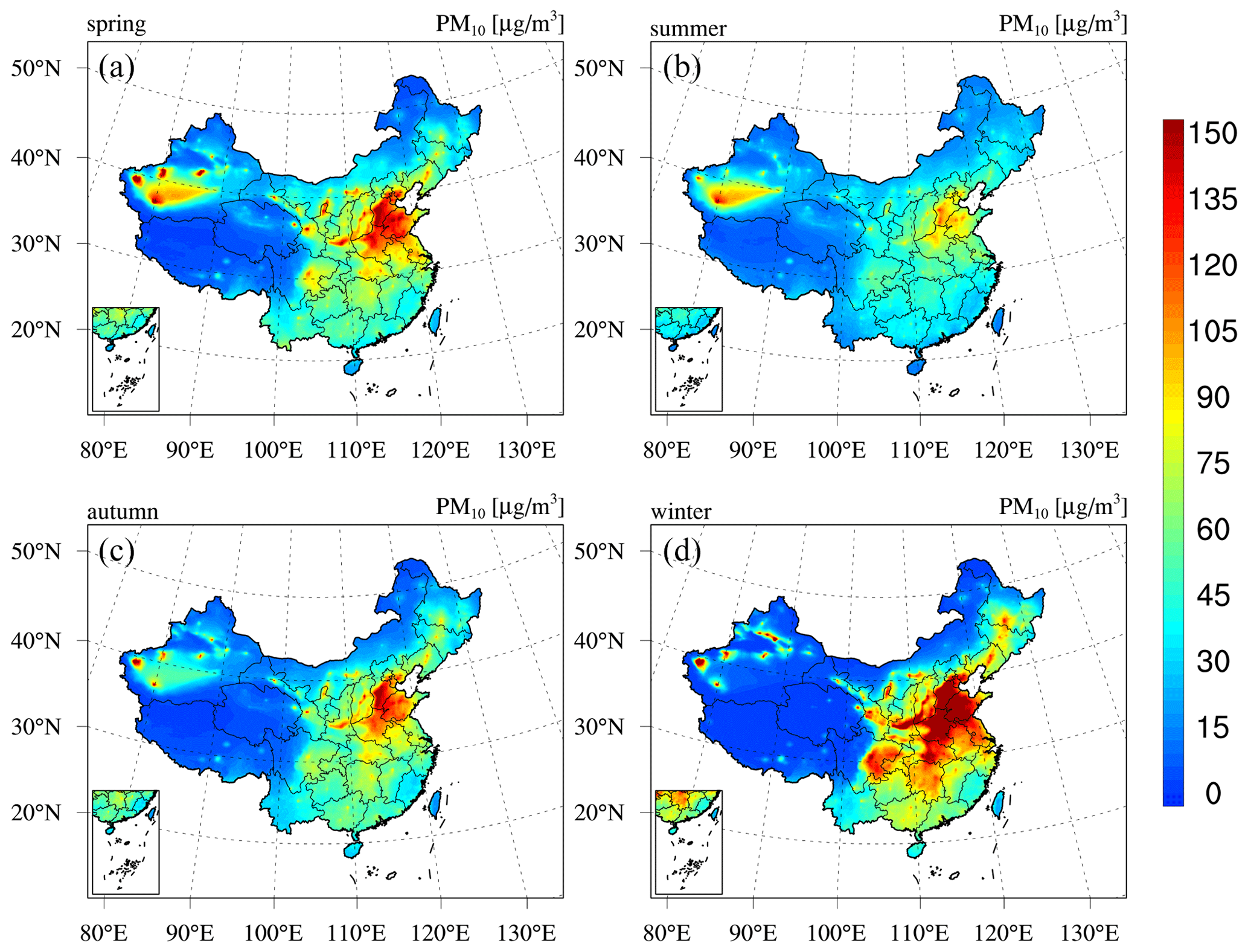
Figure D2Same as Fig. D1 but for PM10.
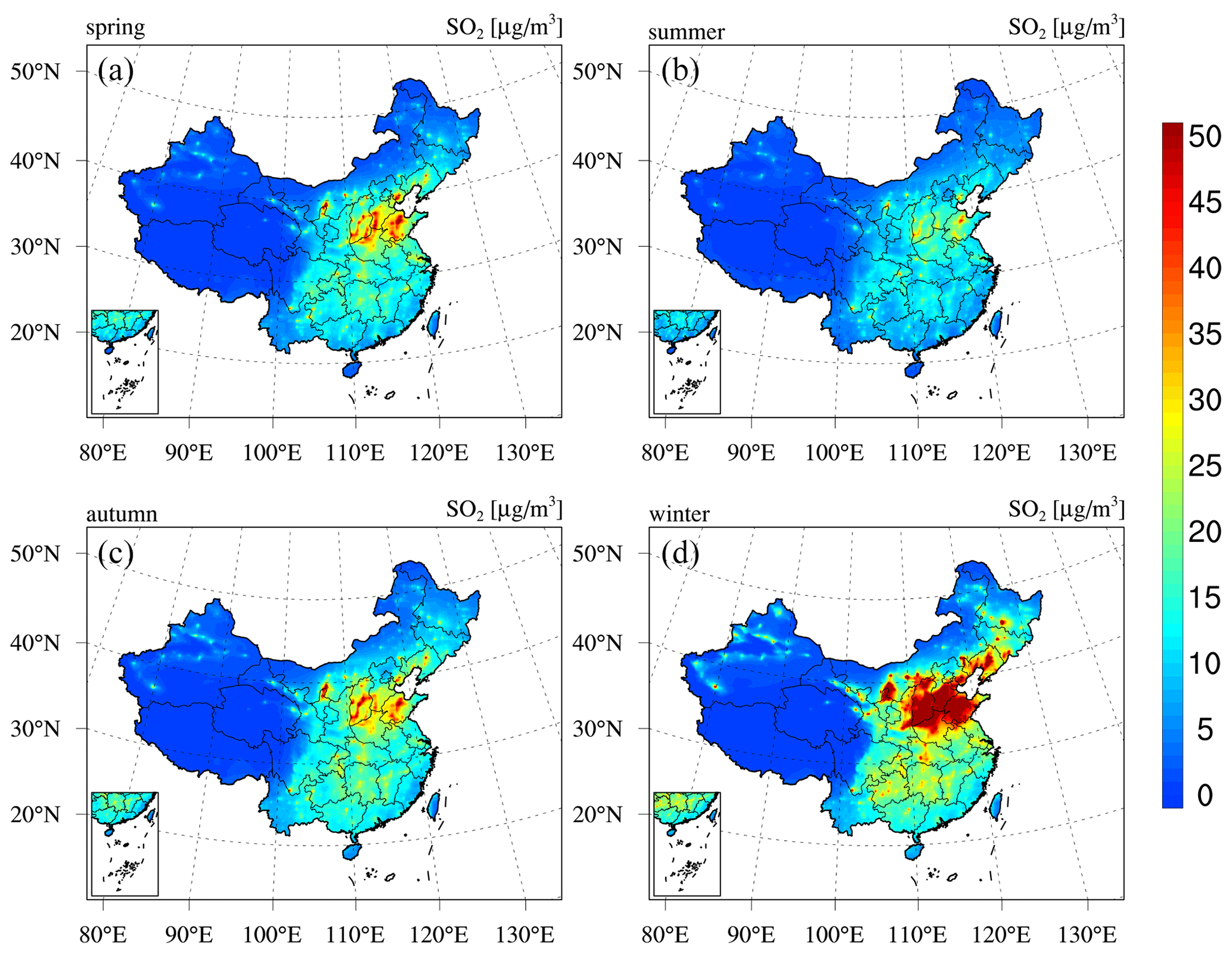
Figure D3Same as Fig. D1 but for SO2.

Figure D4Same as Fig. D1 but for CO.
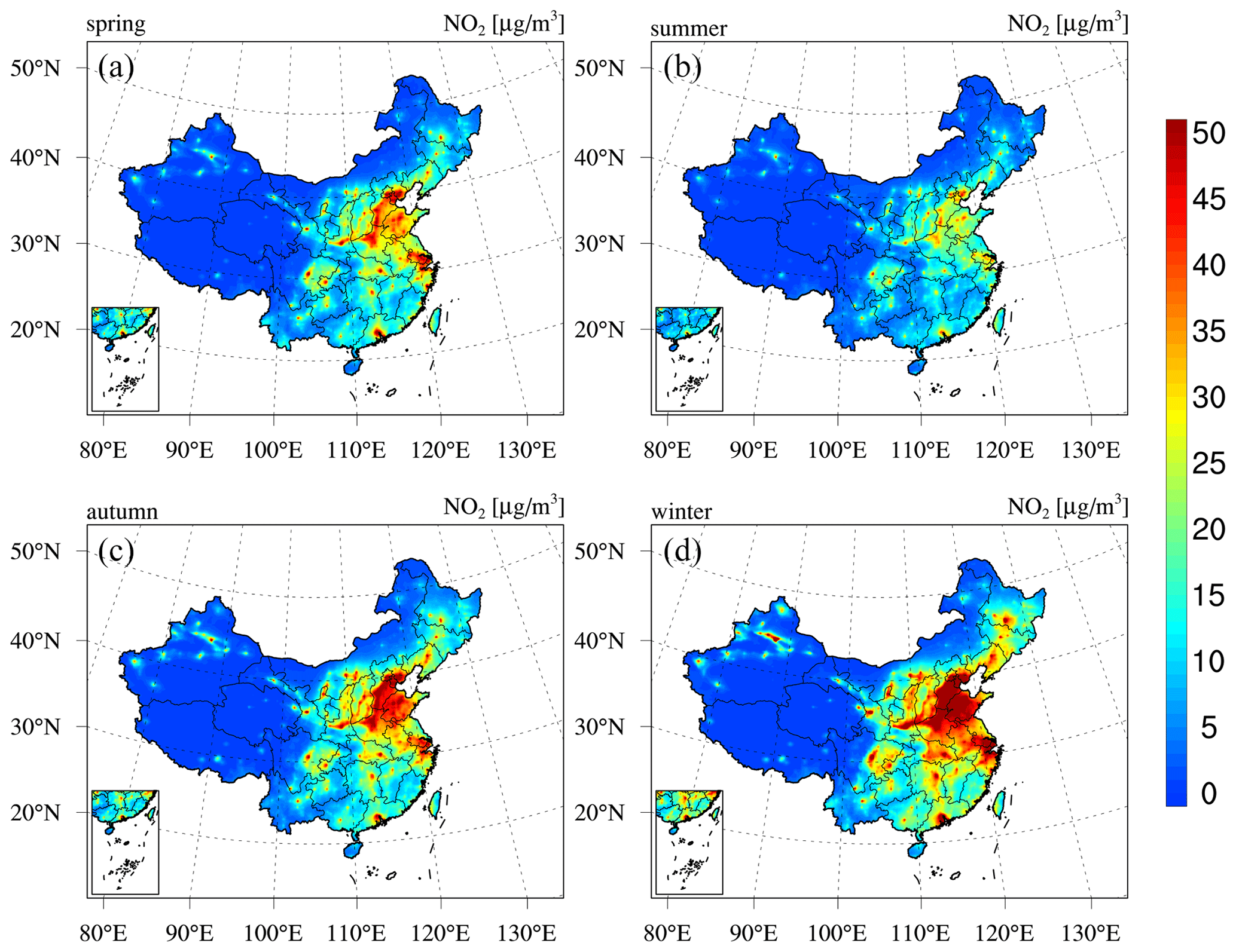
Figure D5Same as Fig. D1 but for NO2.
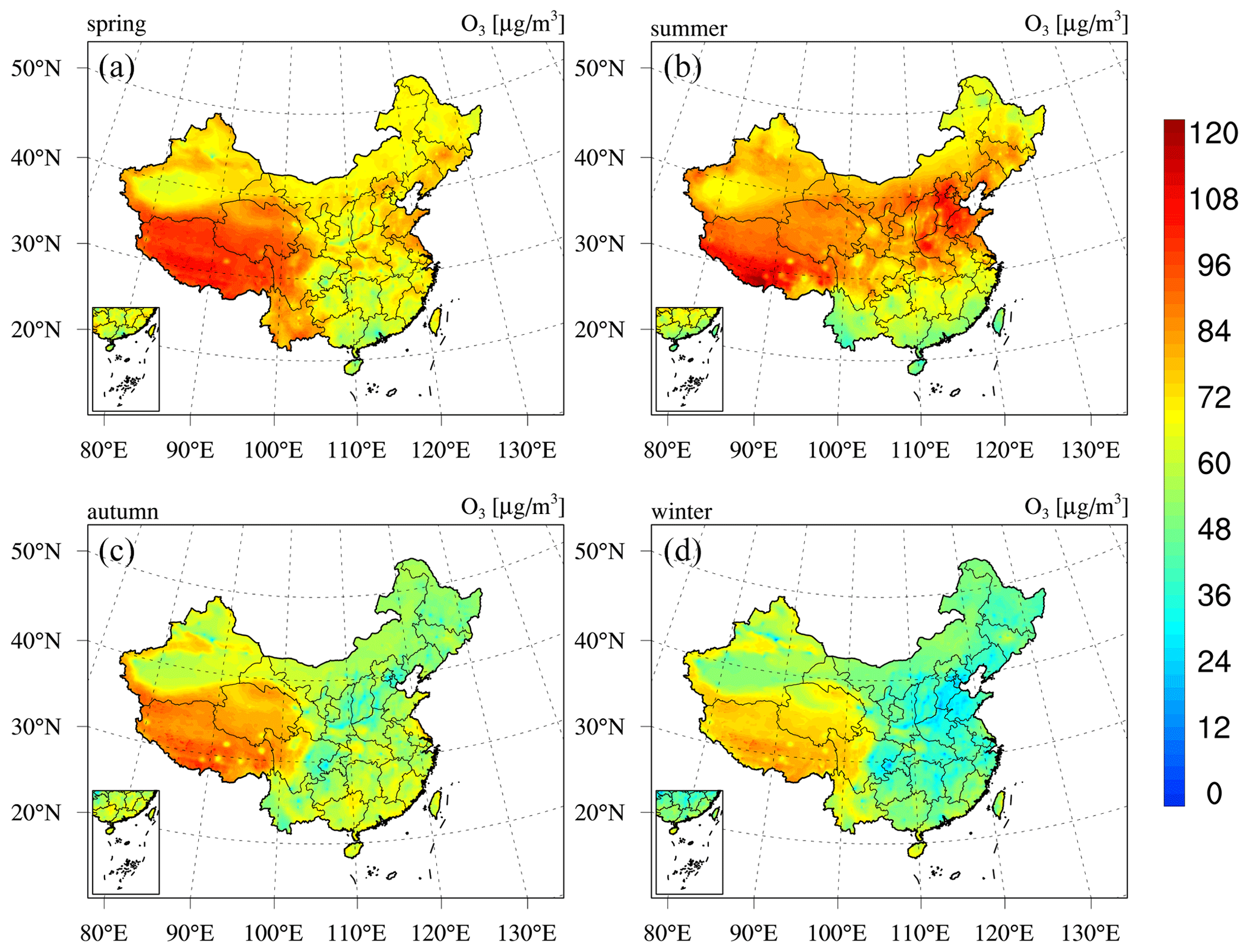
Figure D6Same as Fig. D1 but for O3.
Table E1CV results of the reanalysis (outside brackets) and base simulation (in brackets) for PM2.5 concentrations in different regions of China on different temporal scales.
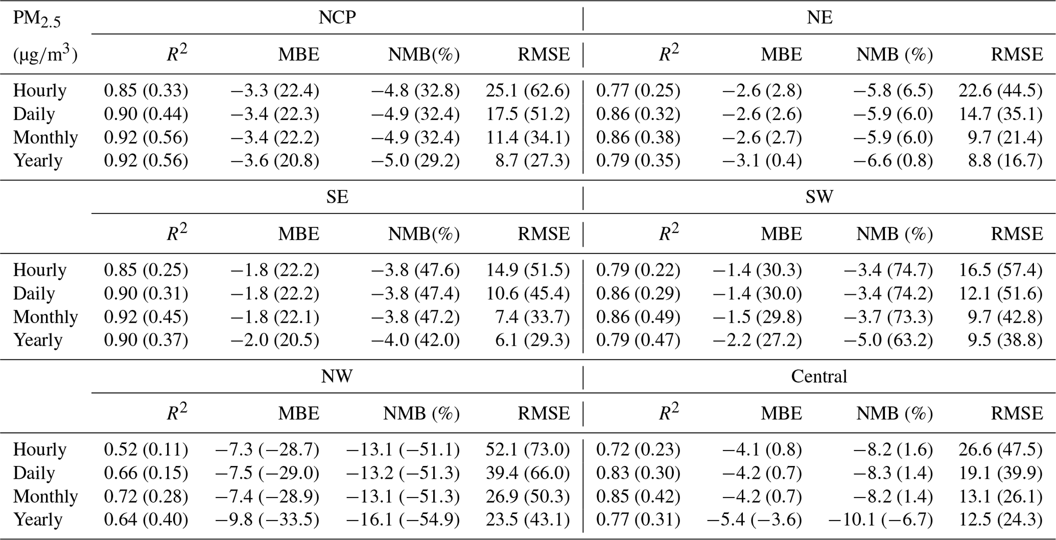
Table E2CV results of the reanalysis (outside brackets) and base simulation (in brackets) for PM10 concentrations in different regions of China on different temporal scales.
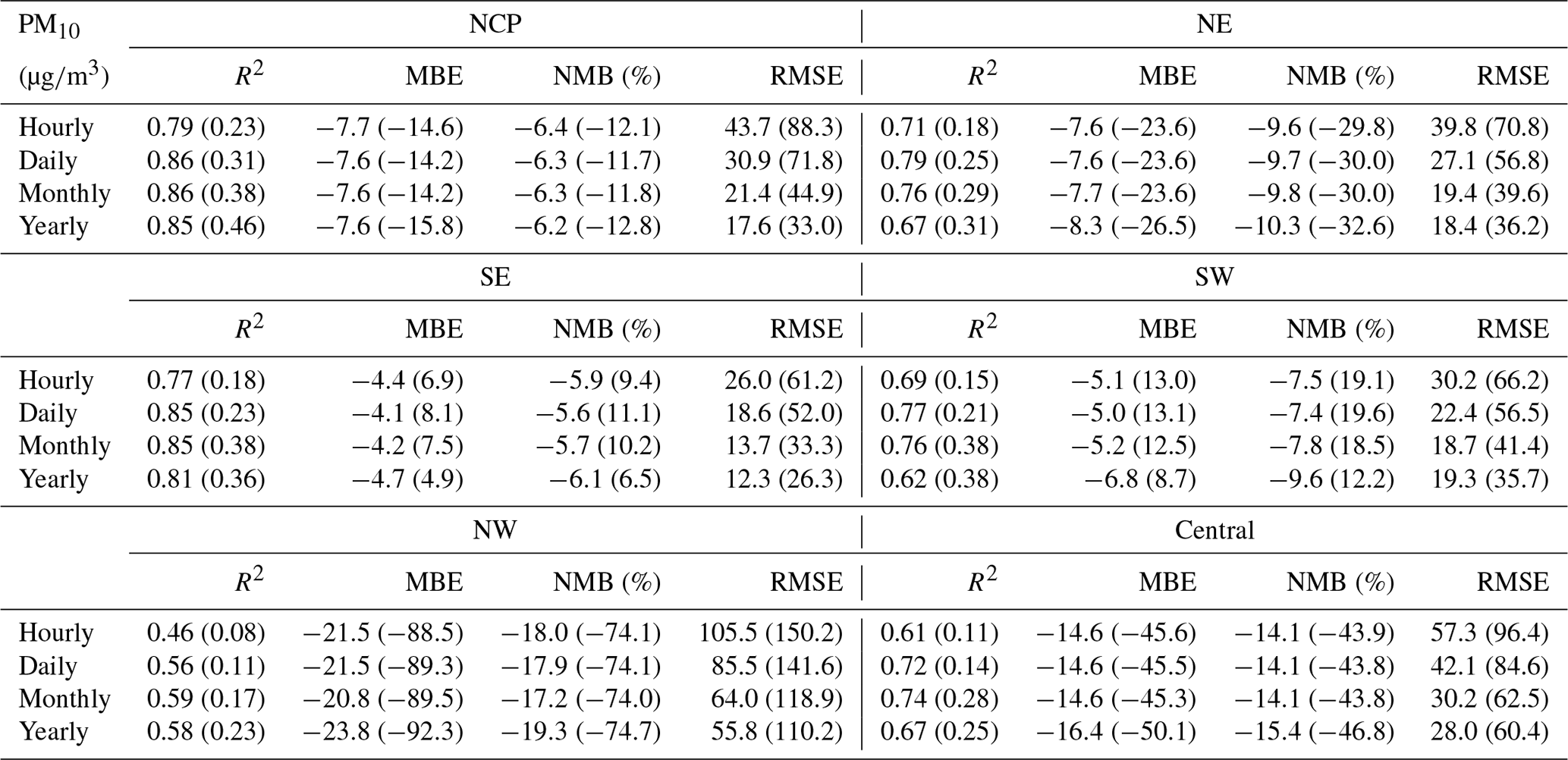
Table E3CV results of the reanalysis (outside brackets) and base simulation (in brackets) for SO2 concentrations in different regions of China on different temporal scales.
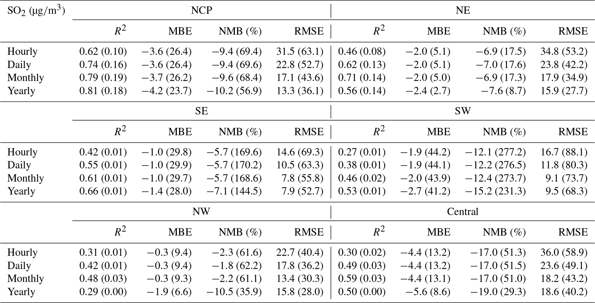
Table E4CV results of the reanalysis (outside brackets) and base simulation (in brackets) for NO2 concentrations in different regions of China on different temporal scales.
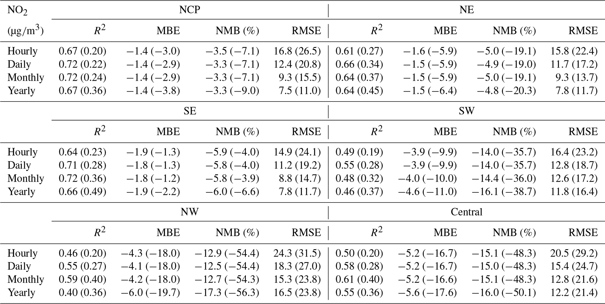
Table E5CV results of the reanalysis (outside brackets) and base simulation (in brackets) for CO concentrations in different regions of China on different temporal scales.
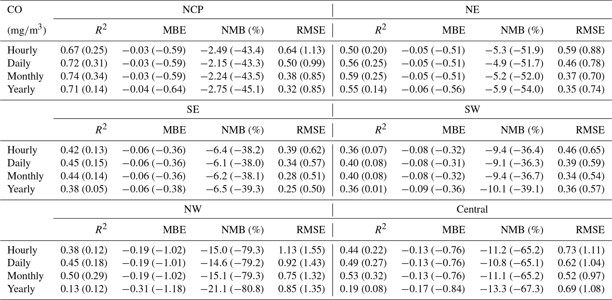
Table E6CV results of the reanalysis (outside brackets) and base simulation (in brackets) for O3 concentrations in different regions of China on different temporal scales.
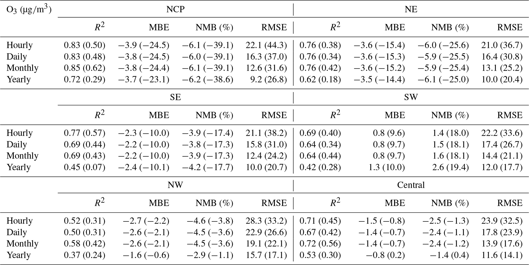
XT, JZ, and ZW conceived and designed the project; HW, LK, XT, and LW established the data assimilation system; QW and LK performed the meteorology simulations; XT, LK, HC, HW, HZ, GJ, and ML conducted the ensemble simulations with the NAQPMS model; JL, LZ, WW, BL, QW, DC, and TS provided the air quality monitoring data; HW executed the quality control of the observation data; FL estimated the representativeness error of the observations; and LK carried out the CAQRA calculations, generated the figures, and wrote the paper, with comments provided by GRC.
The authors declare that they have no conflict of interest.
We acknowledge the use of surface air quality observation data from CNEMC. This study was supported by the National Key Scientific and Technological Infrastructure project “Earth System Science Numerical Simulator Facility” (EarthLab). We would like to thank the editor and the two reviewers for their valuable comments.
This research has been supported by the National Natural Science Foundation of China (grant nos. 91644216, 41575128, and 41875164), the CAS Strategic Priority Research Program (grant no. XDA19040201), and the CAS Information Technology Program (grant no. XXH13506-302).
This paper was edited by David Carlson and reviewed by two anonymous referees.
Athanasopoulou, E., Tombrou, M., Pandis, S. N., and Russell, A. G.: The role of sea-salt emissions and heterogeneous chemistry in the air quality of polluted coastal areas, Atmos. Chem. Phys., 8, 5755–5769, https://doi.org/10.5194/acp-8-5755-2008, 2008.
Barnes, W. L., Pagano, T. S., and Salomonson, V. V.: Prelaunch characteristics of the Moderate Resolution Imaging Spectroradiometer (MODIS) on EOS-AM1, IEEE T. Geosci. Remote, 36, 1088–1100, https://doi.org/10.1109/36.700993, 1998.
Brasseur, G. P., Hauglustaine, D. A., Walters, S., Rasch, P. J., Muller, J. F., Granier, C., and Tie, X. X.: MOZART, a global chemical transport model for ozone and related chemical tracers 1. Model description, J. Geophys. Res.-Atmos., 103, 28265–28289, https://doi.org/10.1029/98jd02397, 1998.
Candiani, G., Carnevale, C., Finzi, G., Pisoni, E., and Volta, M.: A comparison of reanalysis techniques: Applying optimal interpolation and Ensemble Kalman Filtering to improve air quality monitoring at mesoscale, Sci. Total Environ., 458, 7–14, https://doi.org/10.1016/j.scitotenv.2013.03.089, 2013.
Carmichael, G., Sakurai, T., Streets, D., Hozumi, Y., Ueda, H., Park, S., Fung, C., Han, Z., Kajino, M., and Engardt, M.: MICS-Asia II: The model intercomparison study for Asia Phase II methodology and overview of findings, Atmos. Environ., 42, 3468–3490, https://doi.org/10.1016/j.atmosenv.2007.04.007, 2008.
Chen, D., Liu, Z., Ban, J., Zhao, P., and Chen, M.: Retrospective analysis of 2015–2017 wintertime PM2.5 in China: response to emission regulations and the role of meteorology, Atmos. Chem. Phys., 19, 7409–7427, https://doi.org/10.5194/acp-19-7409-2019, 2019.
Chen, G. B., Li, S. S., Knibbs, L. D., Hamm, N. A. S., Cao, W., Li, T. T., Guo, J. P., Ren, H. Y., Abramson, M. J., and Guo, Y. M.: A machine learning method to estimate PM2.5 concentrations across China with remote sensing, meteorological and land use information, Sci. Total Environ., 636, 52–60, https://doi.org/10.1016/j.scitotenv.2018.04.251, 2018.
Chen, Z. Y., Zhang, T. H., Zhang, R., Zhu, Z. M., Yang, J., Chen, P. Y., Ou, C. Q., and Guo, Y. M.: Extreme gradient boosting model to estimate PM2.5 concentrations with missing-filled satellite data in China, Atmos. Environ., 202, 180–189, https://doi.org/10.1016/j.atmosenv.2019.01.027, 2019.
Chu, Y. Y., Liu, Y. S., Li, X. Y., Liu, Z. Y., Lu, H. S., Lu, Y. A., Mao, Z. F., Chen, X., Li, N., Ren, M., Liu, F. F., Tian, L. Q., Zhu, Z. M., and Xiang, H.: A Review on Predicting Ground PM2.5 Concentration Using Satellite Aerosol Optical Depth, Atmosphere-Basel, 7, 25, https://doi.org/10.3390/atmos7100129, 2016.
Cohen, A. J., Brauer, M., Burnett, R., Anderson, H. R., Frostad, J., Estep, K., Balakrishnan, K., Brunekreef, B., Dandona, L., Dandona, R., Feigin, V., Freedman, G., Hubbell, B., Jobling, A., Kan, H., Knibbs, L., Liu, Y., Martin, R., Morawska, L., Pope, C. A., Shin, H., Straif, K., Shaddick, G., Thomas, M., van Dingenen, R., van Donkelaar, A., Vos, T., Murray, C. J. L., and Forouzanfar, M. H.: Estimates and 25-year trends of the global burden of disease attributable to ambient air pollution: an analysis of data from the Global Burden of Diseases Study 2015, Lancet, 389, 1907–1918, https://doi.org/10.1016/s0140-6736(17)30505-6, 2017.
Constantinescu, E. M., Sandu, A., Chai, T. F., and Carmichael, G. R.: Assessment of ensemble-based chemical data assimilation in an idealized setting, Atmos. Environ., 41, 18–36, https://doi.org/10.1016/j.atmosenv.2006.08.006, 2007.
Dee, D. P., Uppala, S. M., Simmons, A. J., Berrisford, P., Poli, P., Kobayashi, S., Andrae, U., Balmaseda, M. A., Balsamo, G., Bauer, P., Bechtold, P., Beljaars, A. C. M., van de Berg, L., Bidlot, J., Bormann, N., Delsol, C., Dragani, R., Fuentes, M., Geer, A. J., Haimberger, L., Healy, S. B., Hersbach, H., Holm, E. V., Isaksen, L., Kallberg, P., Kohler, M., Matricardi, M., McNally, A. P., Monge-Sanz, B. M., Morcrette, J. J., Park, B. K., Peubey, C., de Rosnay, P., Tavolato, C., Thepaut, J. N., and Vitart, F.: The ERA-Interim reanalysis: configuration and performance of the data assimilation system, Q. J. R. Meteor. Soc., 137, 553–597, https://doi.org/10.1002/qj.828, 2011.
Deeter, M. N., Emmons, L. K., Francis, G. L., Edwards, D. P., Gille, J. C., Warner, J. X., Khattatov, B., Ziskin, D., Lamarque, J. F., Ho, S. P., Yudin, V., Attie, J. L., Packman, D., Chen, J., Mao, D., and Drummond, J. R.: Operational carbon monoxide retrieval algorithm and selected results for the MOPITT instrument, J. Geophys. Res.-Atmos., 108, 4399, https://doi.org/10.1029/2002JD003186, 2003.
Elbern, H., Strunk, A., Schmidt, H., and Talagrand, O.: Emission rate and chemical state estimation by 4-dimensional variational inversion, Atmos. Chem. Phys., 7, 3749–3769, https://doi.org/10.5194/acp-7-3749-2007, 2007.
Evensen, G.: Sequential data assimilation with a nonlinear quasi-geostrophic model using Monte Carlo methods to forecast error statistics, J. Geophys. Res.-Oceans, 99, 10143–10162, https://doi.org/10.1029/94JC00572, 1994.
Feng, S. Z., Jiang, F., Jiang, Z. Q., Wang, H. M., Cai, Z., and Zhang, L.: Impact of 3DVAR assimilation of surface PM2.5 observations on PM2.5 forecasts over China during wintertime, Atmos. Environ., 187, 34–49, https://doi.org/10.1016/j.atmosenv.2018.05.049, 2018.
Flemming, J., Benedetti, A., Inness, A., Engelen, R. J., Jones, L., Huijnen, V., Remy, S., Parrington, M., Suttie, M., Bozzo, A., Peuch, V.-H., Akritidis, D., and Katragkou, E.: The CAMS interim Reanalysis of Carbon Monoxide, Ozone and Aerosol for 2003–2015, Atmos. Chem. Phys., 17, 1945–1983, https://doi.org/10.5194/acp-17-1945-2017, 2017.
Gaubert, B., Arellano, A. F., Barre, J., Worden, H. M., Emmons, L. K., Tilmes, S., Buchholz, R. R., Vitt, F., Raeder, K., Collins, N., Anderson, J. L., Wiedinmyer, C., Alonso, S. M., Edwards, D. P., Andreae, M. O., Hannigan, J. W., Petri, C., Strong, K., and Jones, N.: Toward a chemical reanalysis in a coupled chemistry-climate model: An evaluation of MOPITT CO assimilation and its impact on tropospheric composition, J. Geophys. Res.-Atmos., 121, 7310–7343, https://doi.org/10.1002/2016jd024863, 2016.
Granier, C., Lamarque, J., Mieville, A., Muller, J., Olivier, J., Orlando, J., Peters, J., Petron, G., Tyndall, G., and Wallens, S.: POET, a database of surface emissions of ozone precursors, available at: http://www.aero.jussieu.fr/projet/ACCENT/POET.php (last access: 18 February 2021), 2005.
Hanna, S. R., Chang, J. C., and Fernau, M. E.: Monte Carlo estimates of uncertainties in predictions by a photochemical grid model (UAM-IV) due to uncertainties in input variables, Atmos. Environ., 32, 3619–3628, https://doi.org/10.1016/s1352-2310(97)00419-6, 1998.
Hauglustaine, D. A., Brasseur, G. P., Walters, S., Rasch, P. J., Muller, J. F., Emmons, L. K., and Carroll, C. A.: MOZART, a global chemical transport model for ozone and related chemical tracers 2. Model results and evaluation, J. Geophys. Res.-Atmos., 103, 28291–28335, https://doi.org/10.1029/98jd02398, 1998.
Hunt, B. R., Kostelich, E. J., and Szunyogh, I.: Efficient data assimilation for spatiotemporal chaos: A local ensemble transform Kalman filter, Physica D, 230, 112–126, https://doi.org/10.1016/j.physd.2006.11.008, 2007.
Inness, A., Baier, F., Benedetti, A., Bouarar, I., Chabrillat, S., Clark, H., Clerbaux, C., Coheur, P., Engelen, R. J., Errera, Q., Flemming, J., George, M., Granier, C., Hadji-Lazaro, J., Huijnen, V., Hurtmans, D., Jones, L., Kaiser, J. W., Kapsomenakis, J., Lefever, K., Leitão, J., Razinger, M., Richter, A., Schultz, M. G., Simmons, A. J., Suttie, M., Stein, O., Thépaut, J.-N., Thouret, V., Vrekoussis, M., Zerefos, C., and the MACC team: The MACC reanalysis: an 8 yr data set of atmospheric composition, Atmos. Chem. Phys., 13, 4073–4109, https://doi.org/10.5194/acp-13-4073-2013, 2013.
Inness, A., Blechschmidt, A.-M., Bouarar, I., Chabrillat, S., Crepulja, M., Engelen, R. J., Eskes, H., Flemming, J., Gaudel, A., Hendrick, F., Huijnen, V., Jones, L., Kapsomenakis, J., Katragkou, E., Keppens, A., Langerock, B., de Mazière, M., Melas, D., Parrington, M., Peuch, V. H., Razinger, M., Richter, A., Schultz, M. G., Suttie, M., Thouret, V., Vrekoussis, M., Wagner, A., and Zerefos, C.: Data assimilation of satellite-retrieved ozone, carbon monoxide and nitrogen dioxide with ECMWF's Composition-IFS, Atmos. Chem. Phys., 15, 5275–5303, https://doi.org/10.5194/acp-15-5275-2015, 2015.
Inness, A., Ades, M., Agustí-Panareda, A., Barré, J., Benedictow, A., Blechschmidt, A.-M., Dominguez, J. J., Engelen, R., Eskes, H., Flemming, J., Huijnen, V., Jones, L., Kipling, Z., Massart, S., Parrington, M., Peuch, V.-H., Razinger, M., Remy, S., Schulz, M., and Suttie, M.: The CAMS reanalysis of atmospheric composition, Atmos. Chem. Phys., 19, 3515–3556, https://doi.org/10.5194/acp-19-3515-2019, 2019.
Janssens-Maenhout, G., Crippa, M., Guizzardi, D., Dentener, F., Muntean, M., Pouliot, G., Keating, T., Zhang, Q., Kurokawa, J., Wankmüller, R., Denier van der Gon, H., Kuenen, J. J. P., Klimont, Z., Frost, G., Darras, S., Koffi, B., and Li, M.: HTAP_v2.2: a mosaic of regional and global emission grid maps for 2008 and 2010 to study hemispheric transport of air pollution, Atmos. Chem. Phys., 15, 11411–11432, https://doi.org/10.5194/acp-15-11411-2015, 2015.
Jiang, Z. Q., Liu, Z. Q., Wang, T. J., Schwartz, C. S., Lin, H. C., and Jiang, F.: Probing into the impact of 3DVAR assimilation of surface PM10 observations over China using process analysis, J. Geophys. Res.-Atmos., 118, 6738–6749, https://doi.org/10.1002/jgrd.50495, 2013.
Kan, H., Chen, R., and Tong, S.: Ambient air pollution, climate change, and population health in China, Environ. Int., 42, 10–19, https://doi.org/10.1016/j.envint.2011.03.003, 2012.
Kobayashi, S., Ota, Y., Harada, Y., Ebita, A., Moriya, M., Onoda, H., Onogi, K., Kamahori, H., Kobayashi, C., Endo, H., Miyaoka, K., and Takahashi, K.: The JRA-55 Reanalysis: General Specifications and Basic Characteristics, J. Meteorol. Soc. Jpn., 93, 5–48, https://doi.org/10.2151/jmsj.2015-001, 2015.
Kong, L., Tang, X., Zhu, J., Wang, Z., Fu, J. S., Wang, X., Itahashi, S., Yamaji, K., Nagashima, T., Lee, H.-J., Kim, C.-H., Lin, C.-Y., Chen, L., Zhang, M., Tao, Z., Li, J., Kajino, M., Liao, H., Wang, Z., Sudo, K., Wang, Y., Pan, Y., Tang, G., Li, M., Wu, Q., Ge, B., and Carmichael, G. R.: Evaluation and uncertainty investigation of the NO2, CO and NH3 modeling over China under the framework of MICS-Asia III, Atmos. Chem. Phys., 20, 181–202, https://doi.org/10.5194/acp-20-181-2020, 2020.
Kumar, U., De Ridder, K., Lefebvre, W., and Janssen, S.: Data assimilation of surface air pollutants (O3 and NO2) in the regional-scale air quality model AURORA, Atmos. Environ., 60, 99–108, https://doi.org/10.1016/j.atmosenv.2012.06.005, 2012.
Levelt, P. F., Van den Oord, G. H. J., Dobber, M. R., Malkki, A., Visser, H., de Vries, J., Stammes, P., Lundell, J. O. V., and Saari, H.: The Ozone Monitoring Instrument, IEEE T. Geosci. Remote, 44, 1093–1101, https://doi.org/10.1109/TGRS.2006.872333, 2006.
Li, F., Tang, X., Wang, Z., Zhu, L., Wang, X., Wu, H., Lu, M., Li, J., and Zhu, J.: Estimation of Representative Errors of Surface Observations of Air Pollutant Concentrations Based on High-Density Observation Network over Beijing- Tianjin-Hebei Region, Chinese J. Atmos. Sci., 43, 277–284, 2019 (in Chinese with English abstract).
Li, J., Wang, Z., Wang, X., Yamaji, K., Takigawa, M., Kanaya, Y., Pochanart, P., Liu, Y., Irie, H., Hu, B., Tanimoto, H., and Akimoto, H.: Impacts of aerosols on summertime tropospheric photolysis frequencies and photochemistry over Central Eastern China, Atmos. Environ., 45, 1817–1829, https://doi.org/10.1016/j.atmosenv.2011.01.016, 2011.
Li, J., Wang, Z., Zhuang, G., Luo, G., Sun, Y., and Wang, Q.: Mixing of Asian mineral dust with anthropogenic pollutants over East Asia: a model case study of a super-duststorm in March 2010, Atmos. Chem. Phys., 12, 7591–7607, https://doi.org/10.5194/acp-12-7591-2012, 2012.
Li, J., Dong, H. B., Zeng, L. M., Zhang, Y. H., Shao, M., Wang, Z. F., Sun, Y. L., and Fu, P. Q.: Exploring Possible Missing Sinks of Nitrate and Its Precursors in Current Air Quality Models-A Case Simulation in the Pearl River Delta, China, Using an Observation-Based Box Model, Sola, 11, 124–128, https://doi.org/10.2151/sola.2015-029, 2015.
Li, K., Jacob, D. J., Liao, H., Shen, L., Zhang, Q., and Bates, K. H.: Anthropogenic drivers of 2013–2017 trends in summer surface ozone in China, P. Natl. Acad. Sci. USA, 116, 422–427, https://doi.org/10.1073/pnas.1812168116, 2019.
Li, M., Liu, H., Geng, G. N., Hong, C. P., Liu, F., Song, Y., Tong, D., Zheng, B., Cui, H. Y., Man, H. Y., Zhang, Q., and He, K. B.: Anthropogenic emission inventories in China: a review, Natl. Sci. Rev., 4, 834–866, https://doi.org/10.1093/nsr/nwx150, 2017.
Li, T. W., Shen, H. F., Yuan, Q. Q., Zhang, X. C., and Zhang, L. P.: Estimating Ground-Level PM2.5 by Fusing Satellite and Station Observations: A Geo-Intelligent Deep Learning Approach, Geophys. Res. Lett., 44, 11985–11993, https://doi.org/10.1002/2017gl075710, 2017.
Liang, X., Zheng, X. G., Zhang, S. P., Wu, G. C., Dai, Y. J., and Li, Y.: Maximum likelihood estimation of inflation factors on error covariance matrices for ensemble Kalman filter assimilation, Q. J. R. Meteor. Soc., 138, 263–273, https://doi.org/10.1002/qj.912, 2012.
Lin, C. Q., Li, Y., Yuan, Z. B., Lau, A. K. H., Li, C. C., and Fung, J. C. H.: Using satellite remote sensing data to estimate the high-resolution distribution of ground-level PM2.5, Remote Sens. Environ., 156, 117–128, https://doi.org/10.1016/j.rse.2014.09.015, 2015.
Lin, C. Q., Liu, G., Lau, A. K. H., Li, Y., Li, C. C., Fung, J. C. H., and Lao, X. Q.: High-resolution satellite remote sensing of provincial PM2.5 trends in China from 2001 to 2015, Atmos. Environ., 180, 110–116, https://doi.org/10.1016/j.atmosenv.2018.02.045, 2018.
Liu, J. J., Weng, F. Z., and Li, Z. Q.: Satellite-based PM2.5 estimation directly from reflectance at the top of the atmosphere using a machine learning algorithm, Atmos. Environ., 208, 113–122, https://doi.org/10.1016/j.atmosenv.2019.04.002, 2019.
Lu, M. M., Tang, X., Wang, Z. F., Gbaguidi, A., Liang, S. W., Hu, K., Wu, L., Wu, H. J., Huang, Z., and Shen, L. J.: Source tagging modeling study of heavy haze episodes under complex regional transport processes over Wuhan megacity, Central China, Environ. Pollut., 231, 612–621, https://doi.org/10.1016/j.envpol.2017.08.046, 2017.
Lu, Z., Streets, D. G., Zhang, Q., Wang, S., Carmichael, G. R., Cheng, Y. F., Wei, C., Chin, M., Diehl, T., and Tan, Q.: Sulfur dioxide emissions in China and sulfur trends in East Asia since 2000, Atmos. Chem. Phys., 10, 6311–6331, https://doi.org/10.5194/acp-10-6311-2010, 2010.
Ma, C. Q., Wang, T. J., Mizzi, A. P., Anderson, J. L., Zhuang, B. L., Xie, M., and Wu, R. S.: Multiconstituent Data Assimilation With WRF-Chem/DART: Potential for Adjusting Anthropogenic Emissions and Improving Air Quality Forecasts Over Eastern China, J. Geophys. Res.-Atmos., 124, 7393–7412, https://doi.org/10.1029/2019jd030421, 2019.
Ma, Z. W., Hu, X. F., Huang, L., Bi, J., and Liu, Y.: Estimating Ground-Level PM2.5 in China Using Satellite Remote Sensing, Environ. Sci. Technol., 48, 7436–7444, https://doi.org/10.1021/es5009399, 2014.
Ma, Z. W., Hu, X. F., Sayer, A. M., Levy, R., Zhang, Q., Xue, Y. G., Tong, S. L., Bi, J., Huang, L., and Liu, Y.: Satellite-Based Spatiotemporal Trends in PM2.5 Concentrations: China, 2004–2013, Environ. Health Perspect., 124, 184–192, https://doi.org/10.1289/ehp.1409481, 2016.
Menard, R. and Changs, L. P.: Assimilation of stratospheric chemical tracer observations using a Kalman filter. Part II: χ 2-validated results and analysis of variance and correlation dynamics, Mon. Weather Rev., 128, 2672–2686, https://doi.org/10.1175/1520-0493(2000)128<2672:Aoscto>2.0.Co;2, 2000.
Miyazaki, K., Eskes, H. J., Sudo, K., Takigawa, M., van Weele, M., and Boersma, K. F.: Simultaneous assimilation of satellite NO2, O3, CO, and HNO3 data for the analysis of tropospheric chemical composition and emissions, Atmos. Chem. Phys., 12, 9545–9579, https://doi.org/10.5194/acp-12-9545-2012, 2012.
Miyazaki, K., Eskes, H. J., and Sudo, K.: A tropospheric chemistry reanalysis for the years 2005–2012 based on an assimilation of OMI, MLS, TES, and MOPITT satellite data, Atmos. Chem. Phys., 15, 8315–8348, https://doi.org/10.5194/acp-15-8315-2015, 2015.
Miyazaki, K., Bowman, K., Sekiya, T., Eskes, H., Boersma, F., Worden, H., Livesey, N., Payne, V. H., Sudo, K., Kanaya, Y., Takigawa, M., and Ogochi, K.: Updated tropospheric chemistry reanalysis and emission estimates, TCR-2, for 2005–2018, Earth Syst. Sci. Data, 12, 2223–2259, https://doi.org/10.5194/essd-12-2223-2020, 2020.
NBSC: China energy statistical Yearbook, available at: https://navi.cnki.net/KNavi/YearbookDetail?pcode=CYFD&pykm=YCXME&bh= (last access: 19 February 2021), 2017a (in Chinese).
NBSC: China statistical Yearbook on environment, available at: http://www.stats.gov.cn/ztjc/ztsj/hjtjzl/ (last access: 17 April 2020), 2017b (in Chinese).
Nenes, A., Pandis, S. N., and Pilinis, C.: ISORROPIA: A new thermodynamic equilibrium model for multiphase multicomponent inorganic aerosols, Aquat. Geochem., 4, 123–152, https://doi.org/10.1023/a:1009604003981, 1998.
Ott, E., Hunt, B. R., Szunyogh, I., Zimin, A. V., Kostelich, E. J., Corazza, M., Kalnay, E., Patil, D. J., and Yorke, J. A.: A local ensemble Kalman filter for atmospheric data assimilation, Tellus A, 56, 415–428, https://doi.org/10.1111/j.1600-0870.2004.00076.x, 2004.
Pagowski, M. and Grell, G. A.: Experiments with the assimilation of fine aerosols using an ensemble Kalman filter, J. Geophys. Res.-Atmos., 117, 15, https://doi.org/10.1029/2012jd018333, 2012.
Pagowski, M., Grell, G. A., McKeen, S. A., Peckham, S. E., and Devenyi, D.: Three-dimensional variational data assimilation of ozone and fine particulate matter observations: some results using the Weather Research and Forecasting - Chemistry model and Grid-point Statistical Interpolation, Q. J. R. Meteor. Soc., 136, 2013–2024, https://doi.org/10.1002/qj.700, 2010
Peng, Z., Liu, Z., Chen, D., and Ban, J.: Improving PM2.5 forecast over China by the joint adjustment of initial conditions and source emissions with an ensemble Kalman filter, Atmos. Chem. Phys., 17, 4837–4855, https://doi.org/10.5194/acp-17-4837-2017, 2017.
Price, C., Penner, J., and Prather, M.: NOx from lightning .1. Global distribution based on lightning physics, J. Geophys. Res.-Atmos., 102, 5929–5941, https://doi.org/10.1029/96jd03504, 1997.
Qi, J., Zheng, B., Li, M., Yu, F., Chen, C. C., Liu, F., Zhou, X. F., Yuan, J., Zhang, Q., and He, K. B.: A high-resolution air pollutants emission inventory in 2013 for the Beijing-Tianjin-Hebei region, China, Atmos. Environ., 170, 156–168, https://doi.org/10.1016/j.atmosenv.2017.09.039, 2017.
Randerson, J. T., Van Der Werf, G. R., Giglio, L., Collatz, G. J., and Kasibhatla, P. S.: Global Fire Emissions Database, Version 4.1 (GFEDv4), ORNL DAAC, Oak Ridge, Tennessee, USA, https://doi.org/10.3334/ORNLDAAC/1293, 2017.
Randles, C. A., da Silva, A. M., Buchard, V., Colarco, P. R., Darmenov, A., Govindaraju, R., Smirnov, A., Holben, B., Ferrare, R., Hair, J., Shinozuka, Y., and Flynn, C. J.: The MERRA-2 Aerosol Reanalysis, 1980 Onward. Part I: System Description and Data Assimilation Evaluation, J. Climate, 30, 6823–6850, https://doi.org/10.1175/jcli-d-16-0609.1, 2017.
Rienecker, M. M., Suarez, M. J., Gelaro, R., Todling, R., Bacmeister, J., Liu, E., Bosilovich, M. G., Schubert, S. D., Takacs, L., Kim, G. K., Bloom, S., Chen, J. Y., Collins, D., Conaty, A., Da Silva, A., Gu, W., Joiner, J., Koster, R. D., Lucchesi, R., Molod, A., Owens, T., Pawson, S., Pegion, P., Redder, C. R., Reichle, R., Robertson, F. R., Ruddick, A. G., Sienkiewicz, M., and Woollen, J.: MERRA: NASA's Modern-Era Retrospective Analysis for Research and Applications, J. Climate, 24, 3624–3648, https://doi.org/10.1175/jcli-d-11-00015.1, 2011.
Saha, S., Moorthi, S., Pan, H. L., Wu, X. R., Wang, J. D., Nadiga, S., Tripp, P., Kistler, R., Woollen, J., Behringer, D., Liu, H. X., Stokes, D., Grumbine, R., Gayno, G., Wang, J., Hou, Y. T., Chuang, H. Y., Juang, H. M. H., Sela, J., Iredell, M., Treadon, R., Kleist, D., Van Delst, P., Keyser, D., Derber, J., Ek, M., Meng, J., Wei, H. L., Yang, R. Q., Lord, S., Van den Dool, H., Kumar, A., Wang, W. Q., Long, C., Chelliah, M., Xue, Y., Huang, B. Y., Schemm, J. K., Ebisuzaki, W., Lin, R., Xie, P. P., Chen, M. Y., Zhou, S. T., Higgins, W., Zou, C. Z., Liu, Q. H., Chen, Y., Han, Y., Cucurull, L., Reynolds, R. W., Rutledge, G., and Goldberg, M.: The NCEP Climate Forecast System Reanalysis, B. Am. Meteorol. Soc., 91, 1015–1057, https://doi.org/10.1175/2010BAMS3001.1, 2010.
Sakov, P. and Bertino, L.: Relation between two common localisation methods for the EnKF, Comput. Geosci., 15, 225–237, https://doi.org/10.1007/s10596-010-9202-6, 2011.
Shin, M., Kang, Y., Park, S., Im, J., Yoo, C., and Quackenbush, L. J.: Estimating ground-level particulate matter concentrations using satellite-based data: a review, GISci. Remote Sens., https://doi.org/10.1080/15481603.2019.1703288, 57, 1–16, 2019.
Sillman, S.: The relation between ozone, NOx and hydrocarbons in urban and polluted rural environments, Atmos. Environ., 33, 1821–1845, https://doi.org/10.1016/s1352-2310(98)00345-8, 1999.
Silver, B., Reddington, C. L., Arnold, S. R., and Spracklen, D. V.: Substantial changes in air pollution across China during 2015–2017, Environ. Res. Lett., 13, 8, https://doi.org/10.1088/1748-9326/aae718, 2018.
Sindelarova, K., Granier, C., Bouarar, I., Guenther, A., Tilmes, S., Stavrakou, T., Müller, J.-F., Kuhn, U., Stefani, P., and Knorr, W.: Global data set of biogenic VOC emissions calculated by the MEGAN model over the last 30 years, Atmos. Chem. Phys., 14, 9317–9341, https://doi.org/10.5194/acp-14-9317-2014, 2014.
Skamarock, W. C.: A description of the advanced research WRF version 3, Ncar Technical, 113, 7–25, 2008.
Streets, D. G., Bond, T. C., Carmichael, G. R., Fernandes, S. D., Fu, Q., He, D., Klimont, Z., Nelson, S. M., Tsai, N. Y., Wang, M. Q., Woo, J. H., and Yarber, K. F.: An inventory of gaseous and primary aerosol emissions in Asia in the year 2000, J. Geophys. Res.-Atmos., 108, 23, https://doi.org/10.1029/2002jd003093, 2003.
Tang, X., Zhu, J., Wang, Z. F., and Gbaguidi, A.: Improvement of ozone forecast over Beijing based on ensemble Kalman filter with simultaneous adjustment of initial conditions and emissions, Atmos. Chem. Phys., 11, 12901–12916, https://doi.org/10.5194/acp-11-12901-2011, 2011.
Tang, X., Zhu, J., Wang, Z. F., Wang, M., Gbaguidi, A., Li, J., Shao, M., Tang, G. Q., and Ji, D. S.: Inversion of CO emissions over Beijing and its surrounding areas with ensemble Kalman filter, Atmos. Environ., 81, 676–686, https://doi.org/10.1016/j.atmosenv.2013.08.051, 2013.
Tang, X., Zhu, J., Wang, Z., Gbaguidi, A., Lin, C., Xin, J., Song, T., and Hu, B.: Limitations of ozone data assimilation with adjustment of NOx emissions: mixed effects on NO2 forecasts over Beijing and surrounding areas, Atmos. Chem. Phys., 16, 6395–6405, https://doi.org/10.5194/acp-16-6395-2016, 2016.
Tang, X., Kong, L., Zhu, J., Wang, Z. F., Li, J. J., Wu, H. J., Wu, Q. Z., Chen, H. S., Zhu, L. L., Wang, W., Liu, B., Wang, Q., Chen D. H., Pan Y. P., Song, T., Li, F., Zheng, H. T., Jia, G. L., Lu, M. M., Wu, L., and Carmichael, G. R.: A Six-year long High-resolution Air Quality Reanalysis Dataset over China from 2013 to 2018, V2, Sci. Data Bank, https://doi.org/10.11922/sciencedb.00053, 2020a.
Tang, X., Kong, L., Zhu, J., Wang, Z. F., Li, J. J., Wu, H. J., Wu, Q. Z., Chen, H. S., Zhu, L. L., Wang, W., Liu, B., Wang, Q., Chen D. H., Pan Y. P., Song, T., Li, F., Zheng, H. T., Jia, G. L., Lu, M. M., Wu, L., and Carmichael, G. R.: A Six-year long High-resolution Air Quality Reanalysis Dataset over China from 2013 to 2018 (monthly and annual version), V1, Sci. Data Bank, https://doi.org/10.11922/sciencedb.00092, 2020b.
van der A, R. J., Allaart, M. A. F., and Eskes, H. J.: Extended and refined multi sensor reanalysis of total ozone for the period 1970–2012, Atmos. Meas. Tech., 8, 3021–3035, https://doi.org/10.5194/amt-8-3021-2015, 2015.
van der Werf, G. R., Randerson, J. T., Giglio, L., Collatz, G. J., Mu, M., Kasibhatla, P. S., Morton, D. C., DeFries, R. S., Jin, Y., and van Leeuwen, T. T.: Global fire emissions and the contribution of deforestation, savanna, forest, agricultural, and peat fires (1997–2009), Atmos. Chem. Phys., 10, 11707–11735, https://doi.org/10.5194/acp-10-11707-2010, 2010.
van Donkelaar, A., Martin, R. V., Brauer, M., Kahn, R., Levy, R., Verduzco, C., and Villeneuve, P. J.: Global Estimates of Ambient Fine Particulate Matter Concentrations from Satellite-Based Aerosol Optical Depth: Development and Application, Environ. Health Perspect., 118, 847–855, https://doi.org/10.1289/ehp.0901623, 2010.
van Donkelaar, A., Martin, R. V., Brauer, M., Hsu, N. C., Kahn, R. A., Levy, R. C., Lyapustin, A., Sayer, A. M., and Winker, D. M.: Global Estimates of Fine Particulate Matter using a Combined Geophysical-Statistical Method with Information from Satellites, Models, and Monitors, Environ. Sci. Technol., 50, 3762–3772, https://doi.org/10.1021/acs.est.5b05833, 2016.
von Schneidemesser, E., Monks, P. S., Allan, J. D., Bruhwiler, L., Forster, P., Fowler, D., Lauer, A., Morgan, W. T., Paasonen, P., Righi, M., Sindelarova, K., and Sutton, M. A.: Chemistry and the Linkages between Air Quality and Climate Change, Chem. Rev., 115, 3856–3897, https://doi.org/10.1021/acs.chemrev.5b00089, 2015.
Walcek, C. J. and Aleksic, N. M.: A simple but accurate mass conservative, peak-preserving, mixing ratio bounded advection algorithm with FORTRAN code, Atmos. Environ., 32, 3863–3880, https://doi.org/10.1016/S1352-2310(98)00099-5, 1998.
Wang, X. G. and Bishop, C. H.: A comparison of breeding and ensemble transform Kalman filter ensemble forecast schemes, J. Atmos. Sci., 60, 1140–1158, https://doi.org/10.1175/1520-0469(2003)060<1140:Acobae>2.0.Co;2, 2003.
Wang, Z. F., Sha, W. M., and Ueda, H.: Numerical modeling of pollutant transport and chemistry during a high-ozone event in northern Taiwan, Tellus B, 52, 1189–1205, https://doi.org/10.1034/j.1600-0889.2000.01064.x, 2000.
Werner, M., Kryza, M., Pagowski, M., and Guzikowski, J.: Assimilation of PM2.5 ground base observations to two chemical schemes in WRF-Chem – The results for the winter and summer period, Atmos. Environ., 200, 178–189, https://doi.org/10.1016/j.atmosenv.2018.12.016, 2019.
Wesely, M. L.: Parameterization of surface resistances to gaseous dry deposition in regional-scale numerical models, Atmos. Environ., 23, 1293–1304, https://doi.org/10.1016/0004-6981(89)90153-4 1989.
Wu, H. J., Tang, X., Wang, Z. F., Wu, L., Lu, M. M., Wei, L. F., and Zhu, J.: Probabilistic Automatic Outlier Detection for Surface Air Quality Measurements from the China National Environmental Monitoring Network, Adv. Atmos. Sci., 35, 1522–1532, https://doi.org/10.1007/s00376-018-8067-9, 2018.
Xue, T., Zheng, Y. X., Geng, G. N., Zheng, B., Jiang, X. J., Zhang, Q., and He, K. B.: Fusing Observational, Satellite Remote Sensing and Air Quality Model Simulated Data to Estimate Spatiotemporal Variations of PM2.5 Exposure in China, Remote Sens., 9, 19, https://doi.org/10.3390/rs9030221, 2017.
Xue, T., Zheng, Y., Tong, D., Zheng, B., Li, X., Zhu, T., and Zhang, Q.: Spatiotemporal continuous estimates of PM2.5 concentrations in China, 2000–2016: A machine learning method with inputs from satellites, chemical transport model, and ground observations, Environ. Int., 123, 345–357, https://doi.org/10.1016/j.envint.2018.11.075, 2019.
Yan, X. Y., Akimoto, H., and Ohara, T.: Estimation of nitrous oxide, nitric oxide and ammonia emissions from croplands in East, Southeast and South Asia, Glob. Change Biol., 9, 1080–1096, https://doi.org/10.1046/j.1365-2486.2003.00649.x, 2003.
Yao, F., Wu, J., Li, W., and Peng, J.: A spatially structured adaptive two-stage model for retrieving ground-level PM2.5 concentrations from VIIRS AOD in China, ISPRS J. Photogramm., 151, 263–276, https://doi.org/10.1016/j.isprsjprs.2019.03.011, 2019.
You, W., Zang, Z. L., Zhang, L. F., Li, Y., Pan, X. B., and Wang, W. Q.: National-Scale Estimates of Ground-Level PM2.5 Concentration in China Using Geographically Weighted Regression Based on 3 km Resolution MODIS AOD, Remote Sens., 8, 13, https://doi.org/10.3390/rs8030184, 2016.
Yumimoto, K., Tanaka, T. Y., Oshima, N., and Maki, T.: JRAero: the Japanese Reanalysis for Aerosol v1.0, Geosci. Model Dev., 10, 3225–3253, https://doi.org/10.5194/gmd-10-3225-2017, 2017.
Zaveri, R. A. and Peters, L. K.: A new lumped structure photochemical mechanism for large-scale applications, J. Geophys. Res.-Atmos., 104, 30387–30415, https://doi.org/10.1029/1999jd900876, 1999.
Zhan, Y., Luo, Y. Z., Deng, X. F., Chen, H. J., Grieneisen, M. L., Shen, X. Y., Zhu, L. Z., and Zhang, M. H.: Spatiotemporal prediction of continuous daily PM2.5 concentrations across China using a spatially explicit machine learning algorithm, Atmos. Environ., 155, 129–139, https://doi.org/10.1016/j.atmosenv.2017.02.023, 2017.
Zhan, Y., Luo, Y. Z., Deng, X. F., Zhang, K. S., Zhang, M. H., Grieneisen, M. L., and Di, B. F.: Satellite-Based Estimates of Daily NO2 Exposure in China Using Hybrid Random Forest and Spatiotemporal Kriging Model, Environ. Sci. Technol., 52, 4180–4189, https://doi.org/10.1021/acs.est.7b05669, 2018.
Zhang, H. Y., Di, B. F., Liu, D. R., Li, J. R., and Zhan, Y.: Spatiotemporal distributions of ambient SO2 across China based on satellite retrievals and ground observations: Substantial decrease in human exposure during 2013-2016, Environ. Res., 179, 9, https://doi.org/10.1016/j.envres.2019.108795, 2019.
Zhang, Q., Streets, D. G., Carmichael, G. R., He, K. B., Huo, H., Kannari, A., Klimont, Z., Park, I. S., Reddy, S., Fu, J. S., Chen, D., Duan, L., Lei, Y., Wang, L. T., and Yao, Z. L.: Asian emissions in 2006 for the NASA INTEX-B mission, Atmos. Chem. Phys., 9, 5131–5153, https://doi.org/10.5194/acp-9-5131-2009, 2009.
Zheng, B., Chevallier, F., Ciais, P., Yin, Y., Deeter, M. N., Worden, H. M., Wang, Y. L., Zhang, Q., and He, K. B.: Rapid decline in carbon monoxide emissions and export from East Asia between years 2005 and 2016, Environ. Res. Lett., 13, 9, https://doi.org/10.1088/1748-9326/aab2b3, 2018a.
Zheng, B., Tong, D., Li, M., Liu, F., Hong, C., Geng, G., Li, H., Li, X., Peng, L., Qi, J., Yan, L., Zhang, Y., Zhao, H., Zheng, Y., He, K., and Zhang, Q.: Trends in China's anthropogenic emissions since 2010 as the consequence of clean air actions, Atmos. Chem. Phys., 18, 14095–14111, https://doi.org/10.5194/acp-18-14095-2018, 2018b.
Zheng, B., Chevallier, F., Yin, Y., Ciais, P., Fortems-Cheiney, A., Deeter, M. N., Parker, R. J., Wang, Y., Worden, H. M., and Zhao, Y.: Global atmospheric carbon monoxide budget 2000–2017 inferred from multi-species atmospheric inversions, Earth Syst. Sci. Data, 11, 1411–1436, https://doi.org/10.5194/essd-11-1411-2019, 2019.
Zheng, Y. X., Xue, T., Zhang, Q., Geng, G. N., Tong, D., Li, X., and He, K. B.: Air quality improvements and health benefits from China's clean air action since 2013, Environ. Res. Lett., 12, 9, https://doi.org/10.1088/1748-9326/aa8a32, 2017.
Zou, B., Chen, J. W., Zhai, L., Fang, X., and Zheng, Z.: Satellite Based Mapping of Ground PM2.5 Concentration Using Generalized Additive Modeling, Remote Sens., 9, 16, https://doi.org/10.3390/rs9010001, 2017.
- Abstract
- Introduction
- Description of the chemical data assimilation system
- Data assimilation statistics
- Evaluation results
- Data availability
- Conclusions
- Appendix A: Diagnosis results of the outlier detection method
- Appendix B: Inter-species correlation coefficient among different species
- Appendix C: Time series of the OmF and OmA statistics from the data assimilation system
- Appendix D: Spatial distributions of seasonal mean concentrations of different species obtained from CAQRA
- Appendix E: CV results of the reanalysis data in different regions of China
- Author contributions
- Competing interests
- Acknowledgements
- Financial support
- Review statement
- References