A comprehensive and synthetic dataset for global, regional, and national greenhouse gas emissions by sector 1970–2018 with an extension to 2019

To track progress towards keeping global warming well below 2 ^∘C or even 1.5 ^∘C, as agreed in the Paris Agreement, comprehensive up-to-date and reliable information on anthropogenic emissions and removals of greenhouse gas (GHG) emissions is required. Here we compile a new synthetic dataset on anthropogenic GHG emissions for 1970–2018 with a fast-track extension to 2019. Our dataset is global in coverage and includes CO₂ emissions, CH₄ emissions, N₂O emissions, as well as those from fluorinated gases (F-gases: HFCs, PFCs, SF₆, NF₃) and provides country and sector details. We build this dataset from the version 6 release of the Emissions Database for Global Atmospheric Research (EDGAR v6) and three bookkeeping models for CO₂ emissions from land use, land-use change, and forestry (LULUCF). We assess the uncertainties of global greenhouse gases at the 90 % confidence interval (5th–95th percentile range) by combining statistical analysis and comparisons of global emissions inventories and top-down atmospheric measurements with an expert judgement informed by the relevant scientific literature. We identify important data gaps for F-gas emissions. The agreement between our bottom-up inventory estimates and top-down atmospheric-based emissions estimates is relatively close for some F-gas species (∼ 10 % or less), but estimates can differ by an order of magnitude or more for others. Our aggregated F-gas estimate is about 10 % lower than top-down estimates in recent years. However, emissions from excluded F-gas species such as chlorofluorocarbons (CFCs) or hydrochlorofluorocarbons (HCFCs) are cumulatively larger than the sum of the reported species. Using global warming potential values with a 100-year time horizon from the Sixth Assessment Report by the Intergovernmental Panel on Climate Change (IPCC), global GHG emissions in 2018 amounted to 58 ± 6.1 GtCO₂ eq. consisting of CO₂ from fossil fuel combustion and industry (FFI) 38 ± 3.0 GtCO₂, CO₂-LULUCF 5.7 ± 4.0 GtCO₂, CH₄ 10 ± 3.1 GtCO₂ eq., N₂O 2.6 ± 1.6 GtCO₂ eq., and F-gases 1.3 ± 0.40 GtCO₂ eq. Initial estimates suggest further growth of 1.3 GtCO₂ eq. in GHG emissions to reach 59 ± 6.6 GtCO₂ eq. by 2019. Our analysis of global trends in anthropogenic GHG emissions over the past 5 decades (1970–2018) highlights a pattern of varied but sustained emissions growth. There is high confidence that global anthropogenic GHG emissions have increased every decade, and emissions growth has been persistent across the different (groups of) gases. There is also high confidence that global anthropogenic GHG emissions levels were higher in 2009–2018 than in any previous decade and that GHG emissions levels grew throughout the most recent decade. While the average annual GHG emissions growth rate slowed between 2009 and 2018 (1.2 % yr⁻¹) compared to 2000–2009 (2.4 % yr⁻¹), the absolute increase in average annual GHG emissions by decade was never larger than between 2000–2009 and 2009–2018. Our analysis further reveals that there are no global sectors that show sustained reductions in GHG emissions. There are a number of countries that have reduced GHG emissions over the past decade, but these reductions are comparatively modest and outgrown by much larger emissions growth in some developing countries such as China, India, and Indonesia. There is a need to further develop independent, robust, and timely emissions estimates across all gases. As such, tracking progress in climate policy requires substantial investments in independent GHG emissions accounting and monitoring as well as in national and international statistical infrastructures. The data associated with this article (Minx et al., 2021) can be found at https://doi.org/10.5281/zenodo.5566761.

1 Introduction

By signing the Paris Agreement, countries acknowledged the necessity of keeping the most severe climate change risks in check by limiting warming to well below 2 ^∘C and pursuing efforts to limit warming to 1.5 ^∘C (UNFCCC, 2015). This requires rapid and sustained greenhouse gas (GHG) emissions reductions towards net zero carbon dioxide (CO₂) emissions well within the 21st century along with deep reductions in non-CO₂ emissions (Rogelj et al., 2015; IPCC, 2018). Transparent, comprehensive, consistent, accurate, and up-to-date inventories of anthropogenic GHG emissions are crucial for tracking progress by countries, regions, and sectors in moving towards these goals.

However, it is challenging to accurately track the recent GHG performance of countries and sectors. While there is a growing number of global emissions inventories, only a few of them provide a wide coverage of gases, sectors, activities, and countries or regions that are sufficiently up to date to comprehensively track progress and thereby aid discussions in science and policy. Table 1 provides an overview of global emissions inventories. Many inventories focus on individual gases and subsets of activities. Few provide sectoral detail, and particularly for non-CO₂ GHG emissions there is often a considerable time lag in reporting. GHG emissions reporting under the United Nations Framework Convention on Climate Change (UNFCCC) provides reliable, comprehensive, and up-to-date statistics for Annex I countries across all major GHGs. Non-Annex I countries – except the least developed countries and small island states for which this is not mandatory – provide GHG emissions inventory information through biennial update reports (BURs) but with much less stringent reporting requirements in terms of sector, gas, and time coverage (Deng et al., 2021; Gütschow et al., 2016). As a result, many still lack a well-developed statistical infrastructure to provide detailed reports (Janssens-Maenhout et al., 2019).

Here we describe a new, comprehensive, and synthetic dataset for global, regional, and national GHG emissions by sector for 1970–2018 with a fast-track extension to 2019. Our focus is on GHG emissions from anthropogenic activities only. We build the dataset from recent releases of the Emissions Database for Global Atmospheric Research version 6 (EDGARv6) for CO₂ emissions from fossil fuel combustion and industry (FFI), CH₄ emissions, N₂O emissions, and fluorinated gases (F-gases: HFCs, PFCs, SF₆, and NF₃) (Crippa et al., 2021). For completeness we add net CO₂ emissions from land use, land-use change, and forestry (CO₂-LULUCF) from three bookkeeping models (Gasser et al., 2020; Hansis et al., 2015; Houghton and Nassikas, 2017). We provide an assessment of the uncertainties in each GHG at the 90 % confidence interval (5th–95th percentiles) by combining statistical analysis and comparisons of global emissions inventories with an expert judgement informed by the relevant scientific literature.

Table 1 Overview of global inventories of GHG emissions.

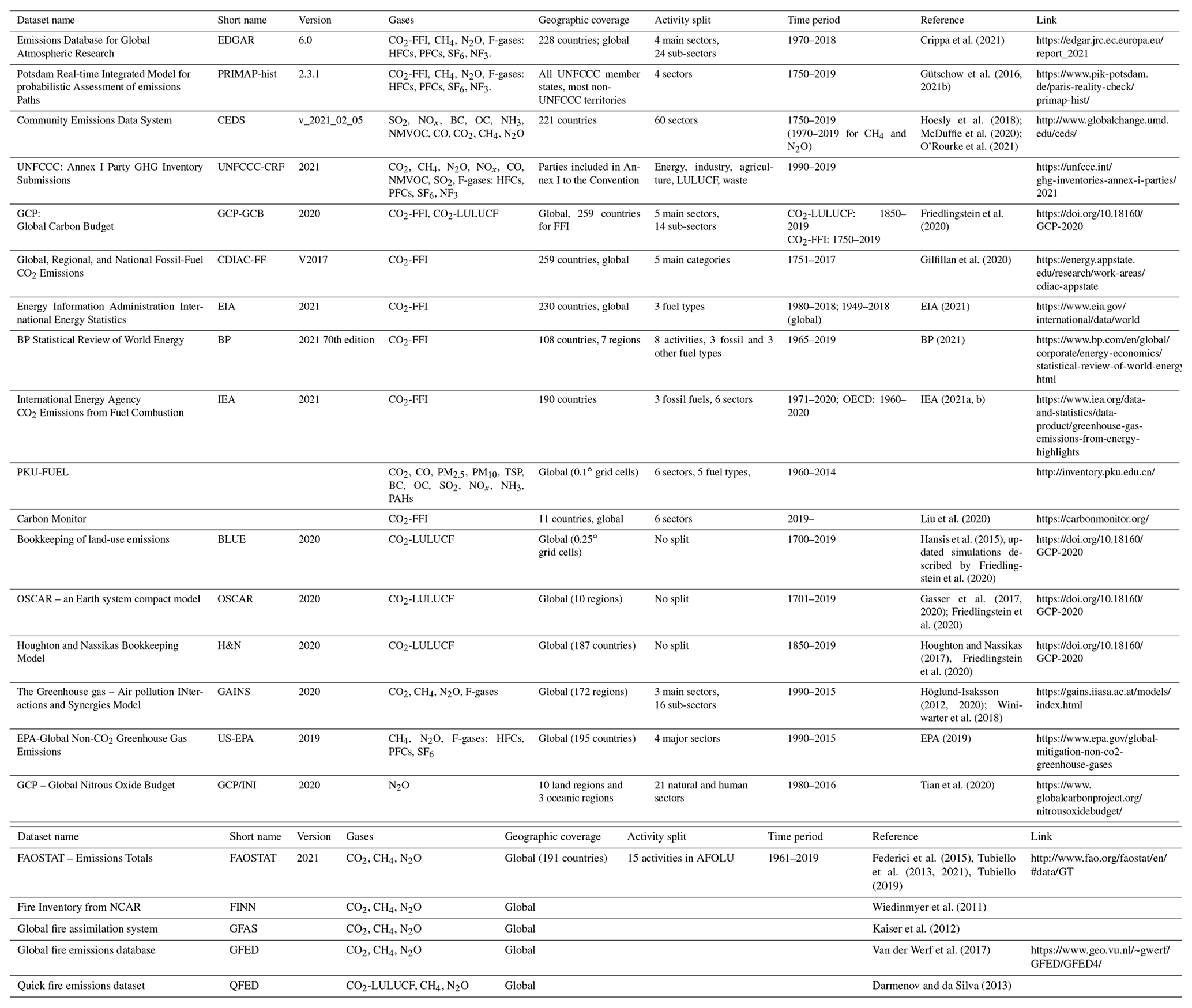
Last access for all URLs: 3 November 2021.

2 Methods and data

2.1 Overview

Our dataset provides a comprehensive, synthetic set of estimates for global GHG emissions disaggregated by 27 economic sectors and 228 countries and territories. Our focus is on anthropogenic GHG emissions: natural sources and sinks are not included. We distinguish between five groups of gases: (1) CO₂ emissions from fossil fuel combustion and industry (CO₂-FFI); (2) CO₂ emissions from land use, land-use change, and forestry (CO₂-LULUCF); (3) methane emissions (CH₄); (4) nitrous oxide emissions (N₂O); (5) fluorinated gases (F-gases) comprising hydrofluorocarbons (HFCs), perfluorocarbons (PFCs), sulfur hexafluoride (SF₆) as well as nitrogen trifluoride (NF₃). F-gases that are internationally regulated as ozone-depleting substances under the Montreal Protocol, such as chlorofluorocarbons (CFCs) and hydrochlorofluorocarbons (HCFCs), are not included. We provide and analyse the GHG emissions data both in native units as well as in CO₂ equivalents (CO₂ eq.) (see Sect. 3.7), as commonly done in wide parts of the climate change mitigation community using global warming potentials with a 100-year time horizon from the IPCC Sixth Assessment Report (AR6) (Forster et al., 2021). We briefly discuss the impact of alternative metric choices in tracking aggregated GHG emissions over the past few decades and juxtapose these estimates of anthropogenic warming.

We report the annual growth rate in emissions E for adjacent years (in percent per year) by calculating the difference between the two years and then normalizing to the emissions in the first year: $\left(\right(E_{(t\mathrm{0}+\mathrm{1})}-E_{t\mathrm{0}})/E_{t\mathrm{0}})\times \mathrm{100}$. We apply a leap-year adjustment where relevant to ensure valid interpretations of annual growth rates. This affects the growth rate by about 0.3 % yr⁻¹ ($\mathrm{1}/\mathrm{366}$) and causes calculated growth rates to go up by approximately 0.3 % if the first year is a leap year and down by 0.3 % if the second year is a leap year. We calculate the relative growth rate in percent per year for multi-year periods (e.g. a decade) by fitting a linear trend to the logarithmic transformation of E across time (see Friedlingstein et al., 2020).

We compile our dataset from four sources: (1) the full EDGARv6 release for CO₂-FFI as well as non-CO₂ GHGs covering the time period 1970–2018 (Crippa et al., 2021); (2) EDGARv6 fast-track data for CO₂-FFI providing preliminary estimates for 2019 (and 2020) (Crippa et al., 2021); (3) CO₂-LULUCF as the average of three bookkeeping models, consistent with the approach of the global carbon project (Friedlingstein et al., 2020); (4) 2019 non-CO₂ emissions based on Olivier and Peters (2020).

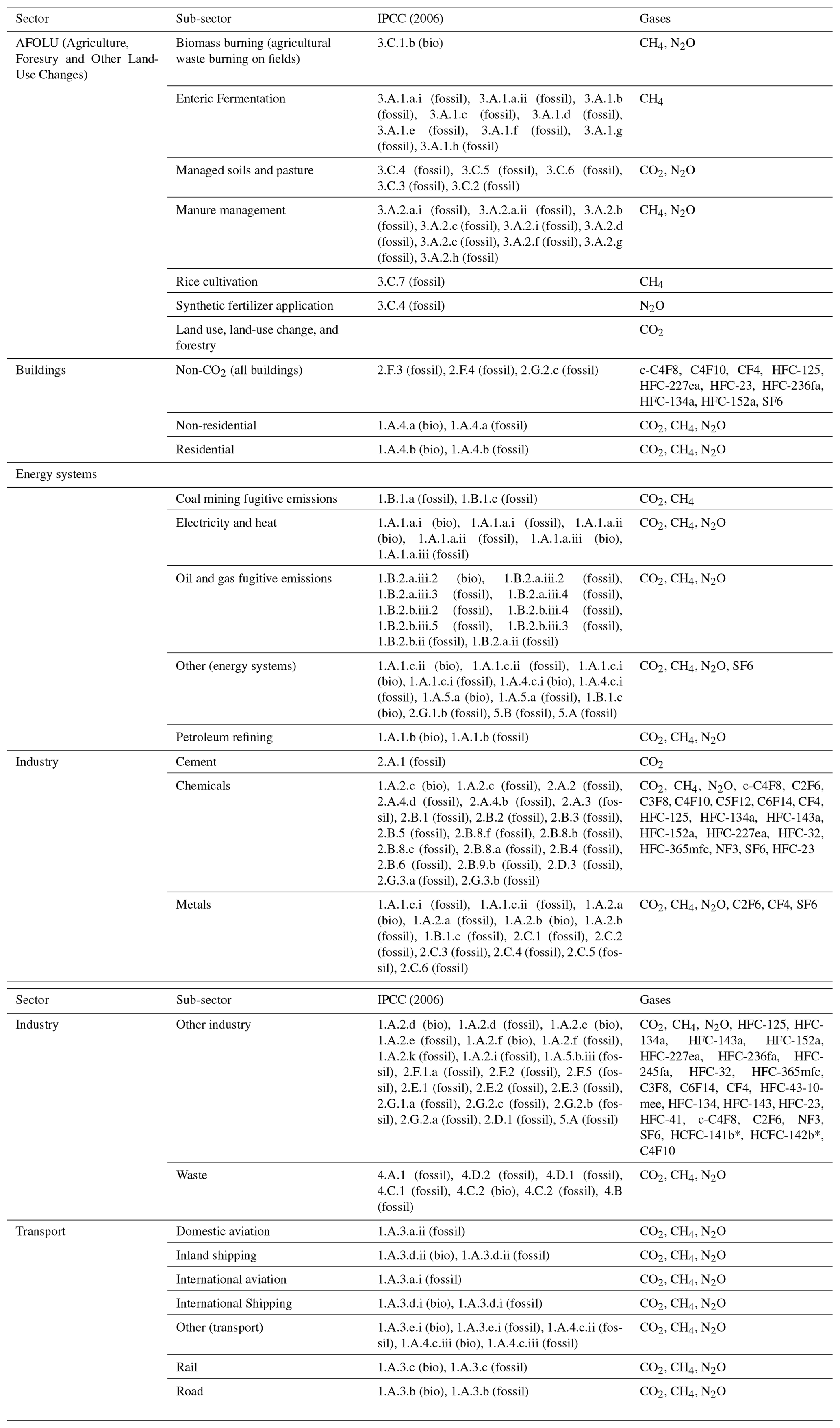
As shown in Table 2, sectoral detail is organized along five major economic sectors as commonly used in IPCC reports on climate change mitigation (IPCC, 2014): energy supply, buildings, transport, industry, as well as Agriculture, Forestry and Other Land-Use Changes (AFOLU). We devise a classification for assigning our 228 countries and territories to regions, combining the standard Annex I/non-Annex I distinction with geographical location. We provide other common regional classifications from the UN and the World Bank as part of the Supplement. The dataset including the sector and region classification can be found at https://doi.org/10.5281/zenodo.5566761 (Minx et al., 2021).

Table 2 Overview of the two-level sector aggregation with reference to assigned source/sink categories conforming to the IPCC reporting guidelines (IPCC, 2006, 2019) as well as relevant GHGs. Note that EDGAR v6 distinguishes between biogenic CO₂ and CH₄ sources with a “bio” label, with all other sectors “fossil” by default, even if that source is not related to fossil fuel activities. The fossil/bio label is hence not descriptive in nature. Two HCFC gases (denoted with ^*) are included in the dataset, despite being neither PFCs nor HFCs (and hence regulated under Montreal). This is to preserve consistency with current and previous versions of EDGAR, which include these gases. Their total warming effect is low (∼ 10 MtCO₂ eq. in 2019), and the major HCFC sources are not included.

2.2 The Emissions Database for Global Atmospheric Research (EDGAR)

EDGAR emissions estimates included in our dataset are derived from the full version 6 release which includes CO₂ and non-CO₂ GHG emissions estimates from 1970 to 2018 computed from stable international statistics and fast-track estimates of fossil CO₂ emissions up to the year 2020 (Crippa et al., 2021). This general EDGAR methodological description is largely taken from Janssens-Maenhout et al. (2019). The EDGAR bottom-up emissions inventory estimates are calculated from international activity data and emissions factors following the 2006 IPCC Guidelines for National Greenhouse Gas Inventories (IPCC, 2006) – updated according to the latest scientific knowledge. Emissions (EMs) from a given sector i in a country C accumulated during a year t for a chemical compound x are calculated with the country-specific activity data (AD), quantifying the activity in sector i, with the mix of j technologies (TECH) and with the mix of k (end-of-pipe) abatement measures (EOP) installed with the share k for each technology j, the emission rate with an uncontrolled emissions factor (EF) for each sector i and technology j and relative reduction (RED) by abatement measure k, as summarized in the following formula:

$$\begin{array}{}\text{(1)}& \begin{array}{rl}& {\mathrm{EM}}_i(C,t,x)={\sum }_{j,k}\left[{\mathrm{AD}}_i\right(C,t)\cdot {\mathrm{TECH}}_{i,j}(C,t)\\ & \cdot {\mathrm{EOP}}_{i,j,k}(C,t)\cdot {\mathrm{EF}}_{i,j}(C,t,x)\\ & \cdot \left(\mathrm{1}-{\mathrm{RED}}_{i,j,k}(C,t,x)\right)].\end{array}\end{array}$$

The activity data are sector dependent and vary from fuel combustion in energy units of a particular fuel type, to the amount of products manufactured, or to the number of animals or the area or yield of cultivated crops. The technology mixes, (uncontrolled) emissions factors and end-of-pipe measures are determined at different levels: country-specific, regional, country group (e.g. Annex I/non-Annex I), or global. Technology-specific emissions factors are used to enable an IPCC Tier-2 approach (see Box 1), taking into account the different management and/technology processes or infrastructures (e.g. different distribution networks) under specific “technologies” and modelling explicitly abatements/emissions reductions, e.g. the CH₄ recovery from coal mine gas at country level under the “end-of-pipe measures”. As with national inventories, emissions are accounted for over a period of 1 calendar year in the country or on the territory in which they took place (i.e. a territorial accounting principle) (IPCC, 2006, 2019). A more complete description of data sources and the methodology for EDGARv6 is provided in Crippa et al. (2021).

To compute emissions up to most recent years, a fast-track methodology is applied, as described in detail in Oreggioni et al. (2021). The underlying idea is to extrapolate trends based on observed activity patterns in representative sectors. For CO₂-FFI emissions, the fast-track estimates were based on the latest BP coal, oil, and natural gas consumption data (BP, 2021). Emission updates for cement, lime, ammonia, and ferroalloys production beyond 2018 are still based on stable statistics and in particular on US Geological Survey statistics, urea production, and consumption on statistics from the International Fertilizer Association, gas used from flaring on data from the Global Gas Flaring Reduction Partnership, steel production on statistics from the World Steel Association, and cement clinker production on UNFCCC data. Fast-track extensions for non-CO₂ GHG emissions are developed from Olivier and Peters (2020). For CH₄ and N₂O these are based on agricultural statistics from the Food and Agricultural Organization (FAO) (CH₄ and N₂O) of the United Nations, fuel production and transmission statistics from IEA and BP (CH₄), as well as data from national greenhouse gas inventory reports on coal production (CH₄ recovery) and the production of chemicals (N₂O abatement) submitted by Annex I countries to the UNFCCC following a common reporting format (CRF) (e.g. UNFCCC, 2021). For F-gases, the fast-track extension was based on the most recent national emissions inventories, submitted under the UNFCCC (up to 2018). For all remaining countries and years, a simple extrapolation was used given the absence of international statistics. We apply these fast-track data by Olivier and Peters (2020) to our dataset by calculating the country- and sector-specific emissions growth between 2018 and 2019 and multiplying it by the 2018 values in our data.

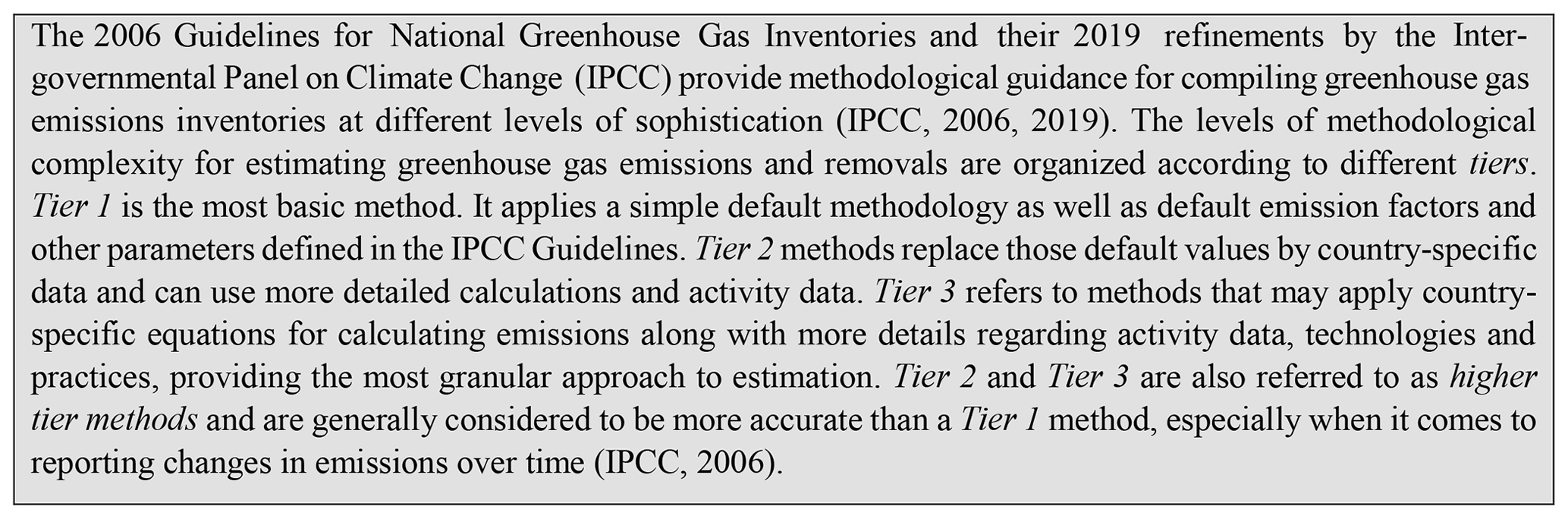
Box 1 Methodological standards for compiling greenhouse gas inventories according to IPCC Guidelines.

2.3 Accounting for CO₂ emissions land use, land-use change, and forestry (CO₂-LULUCF)

We consider all fluxes of CO₂ from land use, land-use change, and forestry. This includes CO₂ fluxes from the clearing of forests and other natural vegetation (by anthropogenic fire and/or clear-cut), afforestation, logging and forest degradation (including harvest activity), shifting cultivation (cycles of forest clearing for agriculture and then abandonment), regrowth of forests and other natural vegetation following wood harvest or abandonment of agriculture, and emissions from peat burning and drainage. Some of these activities lead to emissions of CO₂ to the atmosphere, while others lead to CO₂ sinks. CO₂-LULUCF therefore is the net sum of emissions and removals from all human-induced land-use changes and land management. Note that CO₂-LULUCF is referred to as (net) land-use change emissions, E_LUC, in the context of the Global Carbon Budget (Friedlingstein et al., 2020). Agriculture per se, apart from conversions between different agricultural types, does not lead to substantial CO₂ emissions as compared to land-use changes such as clearing or regrowth of natural vegetation. Therefore, CO₂ fluxes in the AFOLU sector refer mostly to forestry and other land use (changes), while the agricultural part of the sector is mainly characterized by CH₄ and N₂O fluxes.

Since in reality anthropogenic CO₂-LULUCF emissions co-occur with natural CO₂ fluxes in the terrestrial biosphere, models have to be used to distinguish between anthropogenic and natural fluxes (Friedlingstein et al., 2020). CO₂-LULUCF as reported here is calculated via a bookkeeping approach, as originally proposed by Houghton (2003), tracking carbon stored in vegetation and soils before and after land-use change. Response curves are derived from the literature and observations to describe the temporal evolution of the decay and regrowth of vegetation and soil carbon pools for different ecosystems and land-use transitions, including product pools of different lifetimes. These dynamics distinguish bookkeeping models from the common approach of estimating “committed emissions” (assigning all present and future emissions to the time of the land-use-change event), which is frequently derived from remotely sensed land-use area or biomass observations (Ramankutty et al., 2007). Most bookkeeping models also represent the long-term degradation of primary forest as lowered standing vegetation and soil carbon stocks in secondary forests and include forest management practices such as wood harvesting.

The definition of CO₂-LULUCF emissions by global carbon cycle models, as used here and in Canadell et al. (2021b), differs from IPCC definitions (IPCC, 2006) applied in national greenhouse gas inventories (NGHGI) for reporting under the climate convention and, similarly, from FAO estimates of carbon fluxes on forest land (Tubiello et al., 2021). Concretely, this means that NGHGI data include natural terrestrial fluxes caused by changes in environmental conditions, e.g. effects of rising atmospheric CO₂ (“CO₂ fertilization”), climate change, and nitrogen deposition – sometimes called “indirect effects” as opposed to the direct anthropogenic effects of land-use change and management (Houghton et al., 2012) – through adoption of the IPCC so-called land-use proxy approach when they occur in areas that countries declare to be managed. Since environmental changes turned the terrestrial biosphere into a massive sink, removing about one-third of annual anthropogenic emissions in the last decade (Friedlingstein et al., 2020), it is unsurprising that global emissions estimates are smaller based on NGHGI than for global models' definitions (see Fig. 1). About 3.2 GtCO₂ yr⁻¹ (for the period 2005–2014) was found to be explicable by these conceptual differences in anthropogenic forest sink estimation related to the representation of environmental change impacts and the areas considered to be managed (Grassi et al., 2018).

These two conceptually different approaches have different aims. The global models' approach separates natural from anthropogenic drivers, i.e. effects of changes in environmental conditions from effects of land-use change and land management. By contrast, the NGHGI approach separates fluxes based on areas, with all those occurring on managed land being declared anthropogenic. Given that observational data of carbon stocks or fluxes cannot distinguish between the co-occurring effects of environmental changes and land-use activities, an area-based approach that does not require this distinction can more consistently be implemented across countries. These conceptual differences between global models' and NGHGI approaches have been acknowledged (Canadell et al., 2021a; Petrescu et al., 2020a), and approaches have been developed to map the two definitions to each other (Grassi et al., 2018, 2021). For non-CO₂ GHGs, drivers and areas coincide, such that FAOSTAT data for CH₄ and N₂O are complementary to bookkeeping CO₂-LULUCF emissions.

Following the approach taken by the Global Carbon Budget (Friedlingstein et al., 2020), we take the average of estimates from three bookkeeping models: BLUE (Hansis et al., 2015), H&N (Houghton and Nassikas, 2017), and OSCAR (Gasser et al., 2020). Key differences across these estimates, including land-use forcing, are summarized in Table 4. Since bookkeeping models do not include emissions from organic soils, emissions from peat fires and peat drainage are added from external datasets: peat burning is based on the Global Fire Emission Database (GFED4s; van der Werf et al., 2017) and introduces large interannual variability to the CO₂-LULUCF emissions due to synergies of land-use and climate variability, particularly in Southeast Asia, strongly noticeable during El Niño events such as in 1997. Peat drainage is based on estimates by Hooijer et al. (2010) for Indonesia and Malaysia in H&N and added to BLUE and OSCAR from the global FAO data on organic soil emissions from croplands and grasslands (Conchedda and Tubiello, 2020).

3 Uncertainties in GHG emissions estimates

Estimates of historic GHG emissions – CO₂, CH₄, N₂O, and F-gases – are uncertain to different degrees. Assessing and reporting uncertainties is crucial in order to understand whether available estimates are sufficiently accurate to answer, for example, whether GHG emissions are still rising or whether a country has achieved an emissions reduction goal (Marland, 2008). These uncertainties can be of a scientific nature, such as when a process is not sufficiently understood. They also arise from incomplete or unknown parameter information (activity data, emissions factors, etc.) as well as estimation uncertainties from imperfect modelling techniques. There are at least three major ways to examine uncertainties in emissions estimates (Marland et al., 2009): (1) by comparing estimates made by independent methods and observations (e.g. comparing top-down vs. bottom-up estimates; modelling against remote sensing data) (Petrescu et al., 2020a, 2021a, b; Saunois et al., 2020; Tian et al., 2020), (2) by comparing estimates from multiple sources and understanding sources of variation (Andres et al., 2012; Andrew, 2020a; Ciais et al., 2021; Macknick, 2011), and (3) by evaluating multiple estimates from a single source (e.g. Hoesly and Smith, 2018), including approaches such as uncertainty ranges estimated through statistical sampling across parameter values, applied for example at the country or sectoral level (e.g. Andres et al., 2014; Monni et al., 2007; Solazzo et al., 2021) or to spatially distributed emissions (Tian et al., 2019).

Uncertainty estimates can be rather different depending on the method chosen. For example, the range of estimates from multiple sources is bounded by their interdependency; they can be lower than true structural plus parameter uncertainty estimates or than estimates made by independent methods. In particular, it is important to account for potential bias in estimates, which can result from using common methodological or parameter assumptions across estimates, or from missing sources, which can result in a systemic bias in emissions estimates (see N₂O discussion below). Independent top-down observational constraints are, therefore, particularly useful to bound total emissions estimates (Petrescu et al., 2021b, a).

Solazzo et al. (2021) evaluated the uncertainty of the EDGAR source categories and totals for the main GHGs (CO₂-FFI, CH₄, N₂O). This study is based on the propagation of the uncertainty associated with input parameters (activity data and emissions factors) as estimated by expert judgement (Tier-1) and compiled by the IPCC (IPCC, 2006, 2019). A key methodological challenge is determining how well uncertain parameters are correlated between sectors, countries, and regions. The more highly correlated parameters (e.g. emissions factors) are across scales, the higher the resulting overall uncertainty estimate. Solazzo et al. (2021) assume full covariance between the same source categories where similar assumptions are being used, and independence otherwise. For example, they assume full covariance where the same emissions factor is used between countries or sectors while assuming independence where country-specific emissions factors are used. This strikes a balance between extreme assumptions (full independence or full covariance in all cases) that are likely unrealistic but still leans towards higher uncertainty estimates. When aggregating emission sources, assuming full covariance increases the resulting uncertainty estimate. Uncertainties calculated with this methodology tend to be higher than the range of values from ensembles of dependent inventories (Saunois et al., 2016, 2020). The uncertainty of emissions estimates derived from ensembles of gridded results from bio-physical models (Tian et al., 2018) adds an additional dimension of spatial variability and is therefore not directly comparable with aggregate country or regional uncertainty estimated with the methods discussed above.

This section provides an assessment of uncertainties in greenhouse gas emissions data at the global level. The uncertainties reported here combine statistical analysis, comparisons of global emissions inventories, and expert judgement of the likelihood of results lying outside a defined confidence interval, rooted in an understanding gained from the relevant literature. At times, we also use a qualitative assessment of confidence levels to characterize the annual estimates from each term based on the type, amount, quality, and consistency of the evidence as defined by the IPCC (2014).

Such a comprehensive uncertainty assessment covering all major groups of greenhouse gases and considering multiple lines of evidence has been missing in the literature. The absence has provided a serious challenge for transparent, scientific reporting of GHG emissions in climate change assessments like those by the IPCC's Working Group III or the UN Emissions Gap Report that have only more recently started to even deal with the issue (Blanco et al., 2014; UNEP, 2020). Most of the available studies in the peer-reviewed literature using multiple lines of evidence for their assessment have focused on individual gases like in the Global Carbon Budget (Friedlingstein et al., 2020), the Global Methane Budget (Saunois et al., 2020), or the Global Nitrous Oxide Budget (Tian et al., 2020) or covered multiple gases but mainly considered individual lines of evidence (Janssens-Maenhout et al., 2019; Solazzo et al., 2021).

We adopt a 90 % confidence interval (5th–95th percentiles) to report the uncertainties in our GHG emissions estimates; i.e. there is a 90 % likelihood that the true value will be within the provided range if the errors have a Gaussian distribution, and no bias is assumed. This is in line with previous reporting in IPCC AR5 (Blanco et al., 2014; Ciais et al., 2014). We note that national emissions inventories submitted to the UNFCCC are requested to report uncertainty using a 95 % or 2σ confidence interval. The use of this broader uncertainty interval implies, however, a relatively high degree of knowledge about the uncertainty structure of the associated data, particularly regarding the distribution of uncertainty in the tails of the probability distributions. Such a high degree of knowledge is not present across all regions, emission sectors, and species considered here. Note that in some cases below we convert 1σ uncertainty results from the literature to a 90 % confidence interval by implicitly assuming a normal distribution. While we do this as a necessary assumption to obtain a consistent estimate across all GHGs, we note that this itself is an assumption that may not be valid. We have made use of the best available information in the literature but note that much more work on uncertainty quantification remains to be done. Using IPCC uncertainty language, we cannot assign high confidence to the robustness of most existing uncertainty estimates.

3.1 CO₂ emissions from fossil fuels and industrial processes

Several studies have compared estimates of annual CO₂-FFI emissions from different global inventories (Andres et al., 2012; Andrew, 2020a; Gütschow et al., 2016; Janssens-Maenhout et al., 2019; Macknick, 2011; Petrescu et al., 2020b). However, estimates are not fully independent as they all ultimately rely on many of the same data sources. For example, all global inventories use one of four global energy datasets to estimate CO₂ emissions from energy use, and these energy datasets themselves all rely on the same national energy statistics, with few exceptions (Andrew, 2020a). Some divergence between these estimates (see Fig. 1) are related to differences in the estimation methodology, conversion factors, emission coefficients, assumptions about combustion efficiency, and calculation errors (Andrew, 2020a; Marland et al., 2009). Key differences for nine global datasets are highlighted in Table 3 (see also Table 1 for further information on the inventories). Another important source of divergence between datasets is differences in their respective system boundaries (Andres et al., 2012; Andrew, 2020a; Macknick, 2011). Hence, differences across CO₂-FFI emissions estimates do not reflect full uncertainty due to source data dependencies. At the same time, the observed range across estimates from different databases exaggerates uncertainty, to the extent that they largely originate in system boundary differences (Andrew, 2020a; Macknick, 2011).

Across global inventories, mean global annual CO₂-FFI emissions track at 34 ± 2 GtCO₂ in 2014, reflecting a variability of about ±5.4 % (Fig. 1). However, this variability is almost halved when system boundaries are harmonized (Andrew, 2020a). EDGAR CO₂-FFI emissions as used in there track at the top of the range as shown in Fig. 1. This is partly due to the comprehensive system boundaries of EDGAR but also due to the assumption of 100 % oxidation of combusted fuels as per IPCC default assumptions. Once system boundaries are harmonized, EDGAR continues to track at the upper end of the range but no longer at the top. EDGAR CO₂-FFI estimates are further well-aligned with emissions inventories submitted by Annex I countries to the UNFCCC – even though some variation can occur for individual countries such as Kazakhstan, Ukraine, or Estonia, in general, or for certain years (see Fig. S4). Differences in FFI-CO₂ emissions across different versions of the EDGAR dataset are shown in the Supplement (see Fig. S1).

Uncertainties in CO₂-FFI emissions arise from the combination of uncertainty in activity data and uncertainties in emissions factors, including assumptions for combustion completeness and non-combustion uses. CO₂-FFI emissions estimates are largely derived from energy consumption activity data, where data uncertainties are comparatively small due to well-established statistical monitoring systems, although there are larger uncertainties in some countries and time periods (Andres et al., 2012; Andrew, 2020a; Ballantyne et al., 2015; Janssens-Maenhout et al., 2019; Macknick, 2011). Most of the underlying uncertainties are systematic and related to underlying biases in the energy statistics and accounting methods used (Friedlingstein et al., 2020). Uncertainties are lower for fuels with relatively uniform properties such as natural gas, oil, or gasoline and higher for fuels with more diverse properties, such as coal (IPCC, 2006; Blanco et al., 2014). Uncertainties in CO₂ emissions estimates from industrial processes, i.e. non-combustive oxidation of fossil fuels and decomposition of carbonates, are higher than for fossil fuel combustion. At the same time, products such as cement also take up carbon over their life cycle, which are often not fully considered in carbon balances (Guo et al., 2021; Sanjuán et al., 2020; Xi et al., 2016). However, recent versions of the Global Carbon Budget include specific estimates for the cement carbonation sink and estimate average annual CO₂ uptake at 0.70 GtCO₂ for 2010–2019 (Friedlingstein et al., 2020).

Table 3 System boundaries and other key features of global FFI-CO₂ emissions datasets as published. Comparison of some important general characteristics of nine emissions datasets, with bold font indicating a characteristic that might be considered a strength. Columns four to six refer to CO₂ emissions estimates for industrial processes and product use. Since all datasets are under development, these details are subject to change. Further information on the individual inventories can be found in Table 1. Based on Andrew (2020a).

Uncertainties of energy consumption data (and, therefore, CO₂-FFI emissions) are generally higher for the first year of their publication when fewer data are available to constrain estimates. In the BP energy statistics, 70 % of data points are adjusted by an average of 1.3 % of a country's total fossil fuel use in the subsequent year, with further more modest revisions later on (Hoesly and Smith, 2018). Uncertainties are also higher for developing countries, where statistical reporting systems do not have the same level of maturity as in many industrialized countries (Andres et al., 2012; Andrew, 2020b; Friedlingstein et al., 2019, 2020; Gregg et al., 2008; Guan et al., 2012; Janssens-Maenhout et al., 2019; Korsbakken et al., 2016; Marland, 2008). Example estimates of uncertainties for CO₂ emissions from fossil fuel combustion at the 95 % confidence interval are ±3 %–5 % for the US, ±15 %– ± 20 % for China, and ±50 % or more for countries with poorly developed or maintained statistical infrastructure (Andres et al., 2012; Gregg et al., 2008; Marland et al., 1999). However, these customary country groupings do not always predict the extent to which a country's energy data have undergone historical revisions (Hoesly and Smith, 2018). Uncertainties in CO₂-FFI emissions before the 1970s are higher than for more recent estimates. Over the last 2 to 3 decades uncertainties have increased again because of increased production in some developing countries with less rigorous statistics and more uncertain fuel properties (Ballantyne et al., 2015; Friedlingstein et al., 2020; Marland et al., 2009).

The global carbon project (Friedlingstein et al., 2019, 2020; Le Quéré et al., 2018) assesses uncertainties in global anthropogenic CO₂-FFI emissions estimates within 1 standard deviation (1σ) as ±5 % (±10 % at 2σ). This is broadly consistent with the ± 8.4 % uncertainty estimate for CDIAC (Andres et al., 2014) as well as the ±7 %– ± 9 % uncertainty estimate for EDGARv4.3.2 and v5 (Janssens-Maenhout et al., 2019; Solazzo et al., 2021) at 2σ. It remains at the higher end of the ±5 %–± 10 % range provided by Ballantyne et al. (2015). Consistent with the above uncertainty assessments, we present uncertainties for global anthropogenic CO₂ emissions at ±8 % for a 90 % confidence interval, in line with IPCC AR5.

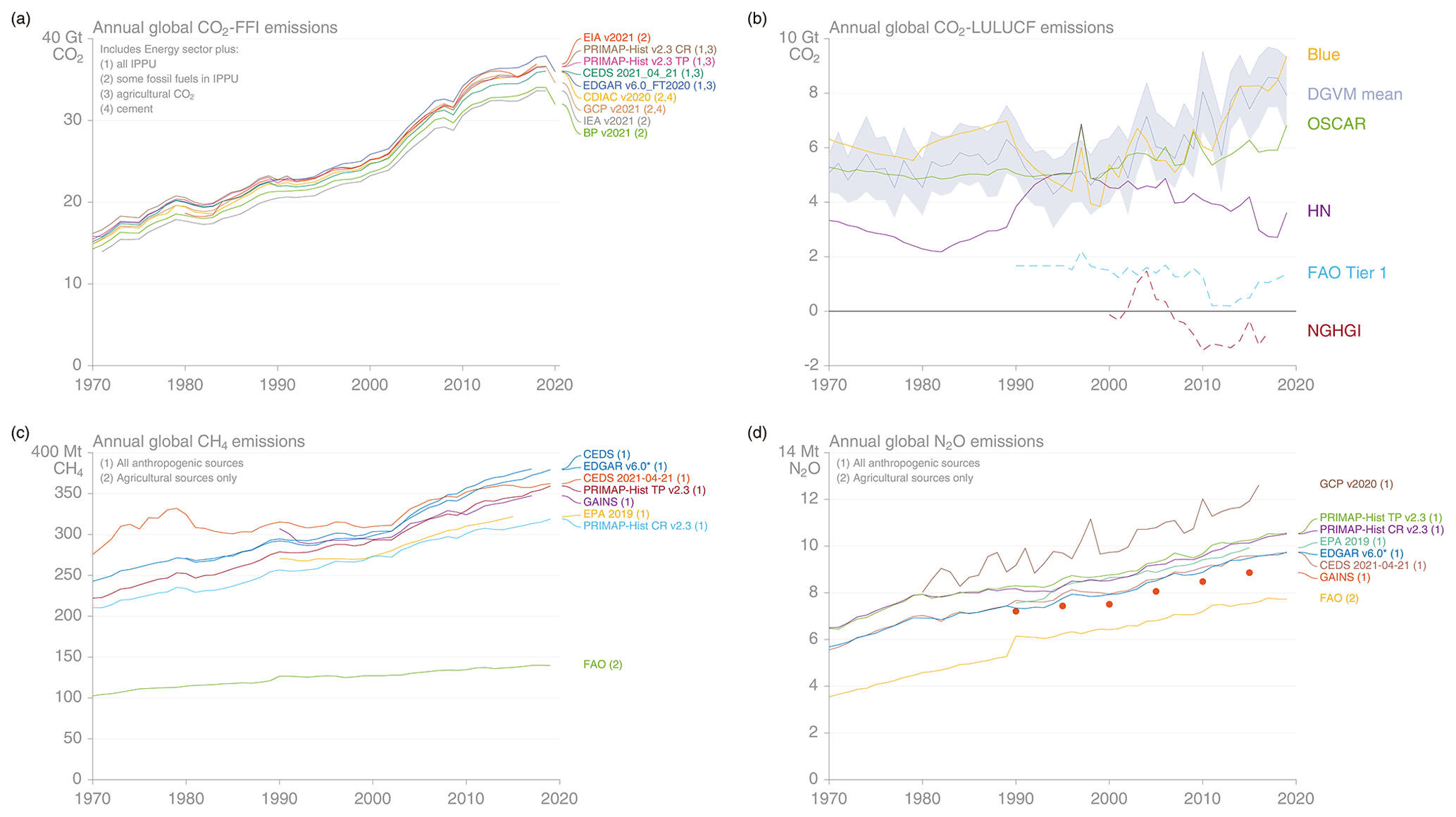
Figure 1 Estimates of global anthropogenic GHG emissions from different data sources for 1970–2019. (a) CO₂ FFI emissions from EDGAR – Emissions Database for Global Atmospheric Research (this dataset) (Crippa et al., 2021), GCP – Global Carbon Project (Andrew and Peters, 2021; Friedlingstein et al., 2020), CEDS – Community Emissions Data System (Hoesly et al., 2018; O'Rourke et al., 2021), CDIAC Global, Regional, and National Fossil-Fuel CO₂ Emissions (Gilfillan et al., 2020), PRIMAP-hist – Potsdam Real-time Integrated Model for probabilistic Assessment of emissions Paths (Gütschow et al., 2016, 2021b), EIA – Energy Information Administration International Energy Statistics (EIA, 2021), BP – BP Statistical Review of World Energy (BP, 2021), and IEA – International Energy Agency (IEA, 2021a, b); IPPU refers to emissions from industrial processes and product use. (b) Net anthropogenic CO₂-LULUCF emissions from BLUE – Bookkeeping of land-use emissions (Friedlingstein et al., 2020; Hansis et al., 2015), DGVM mean – ulti-model mean of CO₂-LULUCF emissions from dynamic global vegetation models (Friedlingstein et al., 2020), OSCAR – an earth system compact model (Friedlingstein et al., 2020; Gasser et al., 2020), and HN – the Houghton and Nassikas Bookkeeping Model (Friedlingstein et al., 2020; Houghton and Nassikas, 2017); for comparison, the net CO₂ flux from FAOSTAT (FAO Tier 1) is plotted, which comprises net emissions and removals on forest land and from net forest conversion (FAOSTAT, 2021; Tubiello et al., 2021), emissions from drained organic soils under cropland/grassland (Conchedda and Tubiello, 2020), and fires in organic soils (Prosperi et al., 2020), as well as a net CO₂ flux estimate from National Greenhouse Gas Inventories (NGHGI) based on country reports to the UNFCCC, which include land use change and fluxes in managed lands (Grassi et al., 2021). (c) Anthropogenic CH₄ emissions from EDGAR (above), CEDS (above), PRIMAP-hist (above); GAINS – the Greenhouse gas–Air pollution Interactions and Synergies Model (Höglund-Isaksson et al., 2020), EPA-2019: Greenhouse gas emissions inventory (US-EPA, 2019), FAO – FAOSTAT inventory emissions (FAOSTAT, 2021; Tubiello, 2018; Tubiello et al., 2013), (d) anthropogenic N₂O emissions from GCP – Global Nitrous Oxide Budget (Tian et al., 2020), CEDS (above), EDGAR (above), PRIMAP-hist (above); GAINS (Winiwarter et al., 2018), EPA-2019 (above), and FAO (above). Differences in emissions across different versions of the EDGAR dataset are shown in the Supplement (Fig. S1).

3.2 Anthropogenic CO₂ emissions from land use, land-use change, and forestry (CO₂-LULUCF)

CO₂-LULUCF emissions are drawn from three global bookkeeping models. For 1990–2019, average net CO₂-LULUCF emissions are estimated at 6.1, 4.3, and 5.6 GtCO₂ yr⁻¹ for BLUE, H&N, and OSCAR (Friedlingstein et al., 2020). Gross emissions 1990–2019 for BLUE, H&N, and OSCAR are 17, 9.6, and 19 GtCO₂ yr⁻¹, while gross removals are 11, 5.3, and 13 GtCO₂ yr⁻¹, respectively. For 1990–2019 maximum average differences are 9.1 and 7.8 GtCO₂ yr⁻¹ for gross emissions and removals, respectively (Friedlingstein et al., 2020). Note that 2016–2019 is extrapolated in H&N and 2019 in OSCAR based on the anomalies of the net flux for the gross fluxes. Differences in the models underlying this observed variability are reported in Table 4. In the longer term, a consistent general upward trend since 1850 across models is reversed during the second part of the 20th century. Since the 1980s, however, differing trends across models have been related to, among other things, different land-use forcings (Gasser et al., 2020). Further differences between BLUE and H&N can be traced in particular to (1) differences in carbon densities between natural and managed vegetation or between primary and secondary vegetation, (2) a higher allocation of cleared and harvested material to fast turnover pools in BLUE compared to H&N, and (3) the inclusion of sub-grid-scale transitions (Bastos et al., 2021).

Uncertainties in CO₂-LULUCF emissions can be more comprehensively assessed through comparisons across a suite of dynamic global vegetation models (DGVMs) (Friedlingstein et al., 2020). DGVMs are not included in the CO₂-LULUCF mean estimate provided here because the typical DGVM setup includes the loss of additional sink capacity, i.e. the additional sink capacity forests could have provided in response to environmental changes, in particular the rise in CO₂, due to their long-lived biomass, but that is lost because large areas of forest were historically cleared for agriculture. The loss of additional sink capacity makes up about 40 % of the DGVM estimate in recent years (Obermeier et al., 2021) and is excluded in bookkeeping estimates. Nonetheless, a CO₂-LULUCF estimate from the DGVM multi-model mean remains consistent with the average estimate from the bookkeeping models, as shown in Fig. 1. Variation across DGVMs is large, with a standard deviation at around 1.8 GtCO₂ yr⁻¹, but is still smaller than the average difference between bookkeeping models at 2.6 GtCO₂ yr⁻¹ as well as the current estimate of H&N (Houghton and Nassikas, 2017) and its previous model versions (Houghton et al., 2012). DGVMs differ in methodology, input data, and how comprehensively they represent land-use-related processes. In particular, land management, such as crop harvesting, tillage, or grazing (all implicitly included in observation-based carbon densities of bookkeeping models), can alter CO₂ flux estimates substantially but is included to varying extents in DGVMs, thus increasing model spread (Arneth et al., 2017). For all types of models, land-use forcing is a major determinant of emissions and removals, and its high uncertainty impacts CO₂-LULUCF estimates (Bastos et al., 2021). The reconstruction of land-use change of the historical past, which has to cover decades to centuries of legacy LULUCF fluxes, is based on sparse data or proxies (Hurtt et al., 2020; Klein Goldewijk et al., 2017), while satellite-based products suffer from complications in distinguishing natural from anthropogenic drivers (Hansen et al., 2013; Li et al., 2018) or accounting for small-scale disturbances and degradation (Matricardi et al., 2020). Lastly, regional carbon budgets can be substantially overestimated or underestimated when the carbon embodied in trade products is not accounted for (Ciais et al., 2021).

We choose Friedlingstein et al. (2020) as the reference point for our uncertainty assessment. The Global Carbon Budget provides a best-value judgement for the ±1σ absolute uncertainty range of CO₂-LULUCF emissions at ±2.6 GtCO₂ yr⁻¹, constant over the last few decades. This constant, absolute uncertainty estimate corresponds roughly to a relative uncertainty of about ±50 % over 1970–2019, which is much higher than for most fossil-fuel-related emissions but reflects the large model spread and large differences between the current estimate of H&N and its previous model versions (Houghton et al., 2012). This corresponds to a relative uncertainty of about ±80 % for a 90 % confidence interval (5th–95th percentiles). However, here we opt for a slightly lower relative uncertainty estimate of about ±70 % for a 90 % confidence interval given that the mean of the CO₂-LULUCF estimates has been increasing over the last few decades. This provides absolute uncertainty estimates that are consistent in magnitude with the constant value in Friedlingstein et al. (2020) over time – slightly lower for earlier years and slightly higher for the most recent years. Compared to IPCC AR5, this is larger than the ±50 % uncertainty estimate applied in the assessment but still in line with the upper end of the broader relative uncertainty range considered of ±50 %–±75 % (Blanco et al., 2014). Finally note that much larger uncertainties in CO₂-LULUCF emissions have been identified across the literature but were traced back to different definitions used in various modelling frameworks (Pongratz et al., 2014) as well as inventory data (Grassi et al., 2018).

Uncertainties can be much higher at a national level than at a global level, since regional biases tend to cancel out. Land-use forcing has been identified as a major driver of differences at regional and global level (Gasser et al., 2020; Hartung et al., 2021; Rosan et al., 2021), as have assumptions about carbon densities and the allocation of cleared or harvested material to slash or product pools of various lifetimes, for which accurate global data over long time periods are missing (Bastos et al., 2021). Although the bookkeeping models are conceptually similar, the bookkeeping estimates include country-specific information to different extents: for example, fire suppression (for the US) is included in H&N (Houghton and Nassikas, 2017) but not the other estimates, and H&N includes peat drainage emissions only for Southeast Asia, while the FAO emissions estimates for organic soil drainage added to BLUE and OSCAR cover all countries (Friedlingstein et al., 2020). The effect of smoothing the FAO cropland and pasture information, which can be very variable in some countries, with a 5-year running mean in H&N, while the annual data are used for the recent decades in HYDE underlying BLUE and OSCAR, must also be expected to contribute to the spread in estimates on a country level. Overall, great care has to be taken when comparing estimates of individual countries across models to not over-interpret differences.

Finally, note that attempts to constrain the estimates of CO₂-LULUCF emissions by observed biomass densities have been undertaken but were successful only in some non-tropical regions (Li et al., 2017). While providing valuable independent and observation-driven information, remote-sensing-derived estimates have limited applicability for model evaluation for the total CO₂-LULUCF flux, since they usually only quantify vegetation biomass changes and exclude legacy emissions from the pre-satellite era. Further, with the exception of the (pan-tropical) estimates by Baccini et al. (2012), they either track committed instead of actual emissions (e.g. Tyukavina et al., 2015), combine a static carbon density map with forest cover changes, or include the natural land sink (e.g. Baccini et al., 2017) to infer fluxes directly from the carbon stock time series – none of which fully distinguishes natural from anthropogenic disturbances.

Table 4 Key differences between global bookkeeping estimates for CO₂-LULUCF emissions. Notes: DGVM – dynamic global vegetation model; LUH2 and FAO refer to land-use forcing datasets; arrows indicate the tendency of a process to increase or decrease emissions compared to the other estimates' choice.

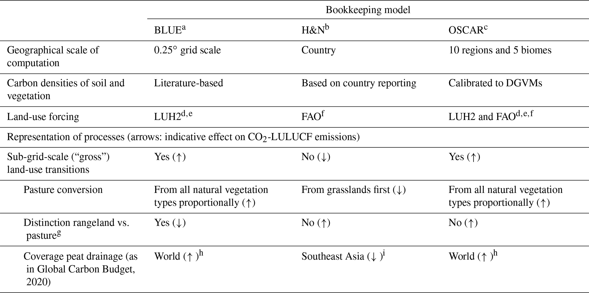
Literature: ^a Hansis et al. (2015), ^b Houghton and Nassikas (2017), ^c Gasser et al. (2020); ^d Hurtt et al. (2020); ^e Chini et al. (2021); ^f FAO (2015); ^g based on rangeland-pasture distinction of the HYDE dataset (Klein Goldewijk et al., 2017) and forest cover map of Hurtt et al. (2020); see Friedlingstein et al. (2020) for details; ^h Conchedda and Tubiello (2020); ⁱ Hooijer et al. (2010)

3.3 Anthropogenic CH₄ emissions

About 60 % of total global CH₄ emissions come from anthropogenic sources (Saunois et al., 2020). These are linked to a range of different sectors: agriculture, fossil fuel production and use, waste, as well as biomass and biofuel burning. Methane emissions can be derived either using bottom-up (BU) estimates that rely on anthropogenic inventories such as EDGAR (Janssens-Maenhout et al., 2019), land surface models that infer part of natural emissions (Wania et al., 2013), or observation-based upscaling for some specific sources such as geological sources (e.g. Etiope et al., 2019). Alternatively, top-down (TD) approaches can be used, such as atmospheric transport models that assimilate methane atmospheric observations to estimate past methane emissions (Houweling et al., 2017). Some TD systems aim to optimize certain emission sectors based on differences in their spatial and temporal distributions (e.g. Bergamaschi et al., 2013), while others only solve for net emissions at the surface. Then the partitioning of TD posterior (output) fluxes between specific source sectors (e.g. Fossil vs. BB&F) is carried out with various degrees of uncertainty depending on the methods and the degree of refinement of sectors but often rely on ratios from the prior knowledge of fluxes. Comprehensive assessments of methane sources and sinks have been provided by Saunois et al. (2016, 2020) and Kirschke et al. (2013).

EDGAR (Crippa et al., 2019, 2021; Janssens-Maenhout et al., 2019) is one of multiple global methane BU inventories available. Other inventories – namely GAINS (Höglund-Isaksson, 2012), US-EPA (EPA, 2011, 2021), CEDS (Hoesly et al., 2018; McDuffie et al., 2020; O'Rourke et al., 2021), PRIMAP-hist (Gütschow et al., 2016, 2021b), and FAOSTAT-CH₄ (Federici et al., 2015; Tubiello, 2018, 2019; Tubiello et al., 2013) – can differ in terms of their country and sector coverage as well as detail. EDGAR, CEDS, US-EPA, and GAINS cover all major source sectors (fossil fuels, agriculture and waste, biofuel) – except large-scale biomass burning – but this can be added from different databases such as FINN (Wiedinmyer et al., 2011), GFAS (Kaiser et al., 2012), GFED (van der Werf et al., 2017), or QFED (Darmenov and da Silva, 2013). Much like CO₂-FFI, these inventories of anthropogenic emissions are not completely independent as they either follow the same IPCC methodology to derive emissions, rely on similar data sources (e.g. FAOSTAT activity data for agriculture, reported fossil fuel production), or draw on reported country inventory data (Petrescu et al., 2020a, e.g. Fig. 4). However, the available estimates will also differ in many ways. For example, while the US-EPA inventory uses the reported emissions by the countries to the UNFCCC, other inventories produce their own estimates using a consistent approach for all countries and country-specific activity data, emissions factors, and technological abatement when available. FAOSTAT and EDGAR mostly apply a Tier-1 approach to estimate CH₄ emissions, while GAINS uses a Tier-2 approach (see Box 1). CEDS is based on pre-existing emissions estimates from FAOSTAT and EDGAR, which are then scaled to match country-specific inventories, largely those reported to the UNFCCC.

Global anthropogenic CH₄ emissions estimates are compared in Fig. 1. EDGARv5 has revised total global CH₄ emissions by about 10 Mt CH₄ yr⁻¹ compared to the previous version due to a higher waste sector estimate (see Fig. S1). Subsequent revisions of the estimation methodology in EDGARv6 in alignment with the IPCC guidelines refinement (IPCC, 2019) lead to very substantial differences in total CH₄ emissions that are up to 50 MtCH₄ yr⁻¹ lower before the 1990s compared to previous versions, but differences are smaller, ranging from 1 to 13 MtCH₄ yr⁻¹ since the 2000s (see Fig. S1). The cause of these differences is a new procedure to separately estimate the venting component for gas and oil in the venting and flaring sector (1B2a/b2). Differences across different versions of the EDGAR dataset are shown in the Supplement (Fig. S1). The US-EPA shows the lowest estimates, probably due to missing estimates from a significant number of countries not reporting to the UNFCCC (US-EPA2020 includes estimates from only 195 countries) and incomplete sectoral coverage. EDGARv6 estimates of anthropogenic CH₄ emissions, as used here, are in the upper range of the different inventories across most anthropogenic sources. However, none of these inventories covers CH₄ emissions from forest and grassland burning, which amount to about 10–12 Mt yr⁻¹ globally.

Saunois et al. (2020) provide estimates of CH₄ sources and sinks based on BU and TD approaches associated with an uncertainty range based on the minimum and maximum values of available studies (because for many individual source and sink estimates the number of studies is often relatively small). Thus, they do not consider the uncertainty of the individual estimates. As shown in Table 5, uncertainties in total global CH₄ emissions across all anthropogenic and natural sources are comparatively small from TD approaches at ±6 % – a range larger than errors in transport models only (Locatelli et al., 2015). However, this uncertainty in total emissions is probably underestimated as the uncertainty in the chemical sink was not fully considered in the TD estimates in Saunois et al. (2020). Uncertainty in the global burden of OH is about ±5 %, much lower than uncertainties derived from detailed analysis using EDGAR data by Janssens-Maenhout (2019) and Solazzo et al. (2021), reaching around ±45 % at 2σ. Saunois et al. (2020) reported uncertainty of 10 %–15 %, which translates to an uncertainty of about ±10 % to ±30 % depending on the category, with larger uncertainty in the fossil fuel sector than in the agriculture and waste sectors (Saunois et al., 2020). However, these uncertainties are also underestimated as they do not consider the uncertainty in each individual estimate, which includes potential uncertainties in activity data, emissions factors, and equations used to estimate emissions.

Uncertainties in EDGAR CH₄ emissions using a Tier-1 approach (see Box 1) are estimated at −33 % to +46 % at 2σ, but there is great variability across individual sectors, ranging from ±30 % (agriculture) to more than ±100 % (fuel combustion), with high uncertainties in oil and gas sector (±93 %) and coal fugitive (±65 %) emissions (Solazzo et al., 2021). National GHG emissions inventories, e.g. for the USA, also report large uncertainties depending on the sector (NASEM, 2018), though the activity data uncertainty may be lower than those for less developed countries. For example, global inventories, such as EDGAR, estimate uncertainties in national anthropogenic emissions of about ±32 % for the 24 member countries of OECD and up to ±57 % for other countries, whose activity data are more uncertain (Janssens-Maenhout et al., 2019).

Table 5 Uncertainties estimated for CH₄ sources at the global scale: based on ensembles of bottom-up (BU) and top-down (TD) estimates, national reports, and specific uncertainty assessments of EDGAR. Note that this table provides uncertainty estimates from some of the key literature based on different methodological approaches. It is not intended to be an exhaustive treatment of the literature.

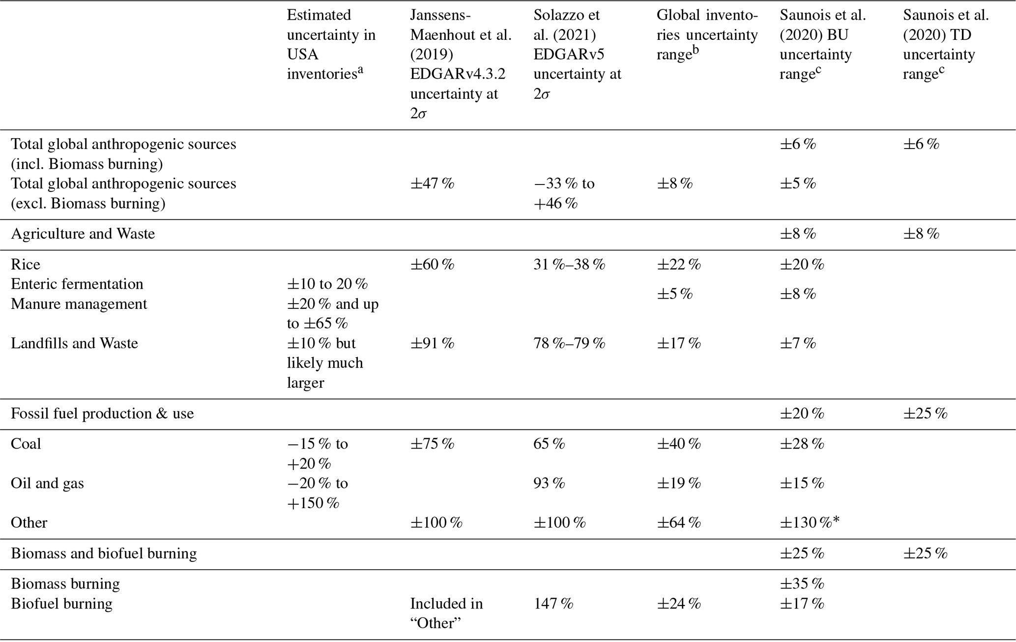
^a Based on NASEM (2018). ^b Uncertainty calculated as $\left(\right(min-max)/\mathrm{2})/\mathrm{mean}\cdot \mathrm{100}$ from the estimates of the year 2017 of the six inventories plotted in Fig. 1. This does not consider the uncertainty on each individual estimate. ^c Uncertainty calculated as $\left(\right(min-max)/\mathrm{2})/\mathrm{mean}\cdot \mathrm{100}$ from individual estimates for the 2008–2017 decade. This does not consider the uncertainty on each individual estimate, which is probably larger than the range presented here. ^∗ Mainly due to difficulties in attributing emissions to a small specific emission sector.

The 2020 UN emissions gap report (UNEP, 2020) gives an uncertainty range for global anthropogenic CH₄ emissions with 1 standard deviation of ±30 % (i.e. ±60 % for 2σ). On the other hand, IPCC AR5 provides a comparatively low estimate at ± 20 % for a 90 % confidence interval. Overall, we apply a best value judgment of ±30 % for global anthropogenic CH₄ emissions for a 90 % confidence interval. This is justified by the larger uncertainties reported in studies on the EDGAR dataset (Janssens-Maenhout et al., 2019; Solazzo et al., 2021) as well as for FAO activity statistics by Tubiello et al. (2015).

3.4 Anthropogenic N₂O emissions

Anthropogenic N₂O emissions occur in a number of sectors, namely agriculture, fossil fuel and industry, biomass burning, and waste. The emissions from the agriculture sector have four components: direct and indirect emissions from soil and water bodies (inland, coastal, and oceanic waters), manure left on pasture, manure management, and aquaculture. Besides these main sectors, a final “other” category represents the sum of the effects of climate, elevated atmospheric CO₂, and land cover change. This is a new sector that was developed as part of the Global Nitrous Oxide Budget (Tian et al., 2020) – a recent assessment to quantify all sources and sinks of N₂O emissions updating previous work (Kroeze et al., 1999; Mosier et al., 1998; Mosier and Kroeze, 2000; Syakila and Kroeze, 2011). We will refer to estimates from the Global Nitrous Oxide Budget as GCP-N₂O as the assessment facilitated by the Global Carbon Project (GCP). Overall, anthropogenic sources contributed just over 40 % to total global N₂O emissions (Tian et al., 2020).

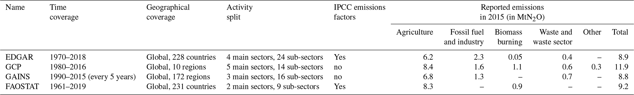
There are a variety of approaches for estimating N₂O emissions. These include inventories (Janssens-Maenhout et al., 2019; Tian et al., 2018; Tubiello et al., 2013), statistical extrapolations of flux measurements (Wang et al., 2020), and process-based land and ocean modelling (Tian et al., 2019; Yang et al., 2020). There are at least five relevant global N₂O emissions inventories available: EDGAR (Crippa et al., 2019, 2021; Janssens-Maenhout et al., 2019), GAINS (Winiwarter et al., 2018), FAOSTAT-N₂O (Tubiello, 2018; Tubiello et al., 2013), CEDS (Hoesly et al., 2018; McDuffie et al., 2020; O'Rourke et al., 2021), PRIMAP-hist (Gütschow et al., 2016, 2021b), and GFED (van der Werf et al., 2017). While EDGAR and GAINS cover all sectors except biomass burning, FAOSTAT-N₂O is focused on agriculture and biomass burning and GFED on biomass burning only. As shown in Fig. 1, EDGAR, GAINS, CEDS, and FAOSTAT emissions are consistent in magnitude and trend. Recent revisions in estimating indirect N₂O emissions in EDGARv6 lead to an average increase of 1.5 % yr⁻¹ in total N₂O emissions estimates between 1999 and 2018 compared to the two previous versions (differences before 1999 were negligible at less than 1 % yr⁻¹). Differences across different versions of the EDGAR dataset are shown in the Supplement (Fig. S1). The main discrepancies across different global inventories are in agriculture, where emissions estimates from the Global Nitrous Oxide Budget and FAOSTAT are on average 1.5 Mt N₂O yr⁻¹ higher than those from GAINS and EDGAR during 1990–2016 due to higher estimates of direct emissions from fertilized soils and manure left on pasture. GCP-N₂O provides the largest estimate (Fig. 1) – because it was synthesized from the other three inventories and further informed by additional bottom-up modelling estimates – and is as such more comprehensive in scope due to the new sector discussed above. EDGAR estimates of anthropogenic N₂O emissions as used in this dataset should therefore be considered lower-bound estimates (see also Table 6). Differences in N₂O emissions across different versions of EDGAR are shown in Fig. S1.

Anthropogenic N₂O emissions estimates are subject to considerable uncertainty – larger than those from FFI-CO₂ or CH₄ emissions. N₂O inventories suffer from high uncertainty on input data, including fertilizer use, livestock manure availability, storage, and applications (Galloway et al., 2010; Steinfeld et al., 2010), as well as nutrient, crop, and soil management (Ciais et al., 2014; Shcherbak et al., 2014). Emissions factors are also uncertain (Crutzen et al., 2008; Hu et al., 2012; IPCC, 2019; Yuan et al., 2019), and there remain several sources that are not yet well understood (e.g. peatland degradation, permafrost) (Elberling et al., 2010; Wagner-Riddle et al., 2017; Winiwarter et al., 2018). Model-based estimates face uncertainties associated with the specific model configuration as well as parametrization (Buitenhuis et al., 2018; Tian et al., 2018, 2019). Total uncertainty is also large because N₂O emissions are dominated by emissions from soils, where our level of process understanding is rapidly changing.

For EDGAR, uncertainties in N₂O emissions are estimated based on default values (IPCC, 2006) at ±42 % for 24 OECD90 countries and at ±93 % for other countries for a 95 % confidence interval (Janssens-Maenhout et al., 2019). However, Solazzo et al. (2021) arrive at substantially larger values, allowing for correlation of uncertainties between sectors, countries, and regions. At a sector level, uncertainties are larger for agriculture (263 %) than for energy (113 %), waste (181 %), industrial processes and product use (14 %), and other (112 %). In the recent Emissions Gap Report (UNEP, 2020), relative uncertainties for global anthropogenic N₂O emissions are estimated at ±50 % for a 68 % (1σ) confidence interval. This is larger than the ±60 % uncertainties reported in IPCC AR5 for a 90 % confidence interval (Blanco et al., 2014) but is comparable with the ranges for anthropogenic emissions in the Global N₂O Budget (Tian et al., 2020). Overall, we assess the relative uncertainty for global anthropogenic N₂O emissions at ±60 % for a 90 % confidence interval.

Table 6 Comparison of four global N₂O inventories: EDGAR (Crippa et al., 2021); GCP (Tian et al., 2020); GAINS (Winiwarter et al., 2018); FAOSTAT (FAOSTAT, 2021; Tubiello, 2018; Tubiello et al., 2013).

3.5 Fluorinated gases

Fluorinated gases comprise over a dozen different species that are primarily used as refrigerants, solvents, and aerosols. Here we compare global emissions of F-gases estimated in EDGAR to top-down estimates from the 2018 World Meteorological Organisation's (WMO) Scientific Assessment of Ozone Depletion (Engel and Rigby, 2018; Montzka and Velders, 2018). We provide additional comparisons with other EDGAR versions as well as estimates by the US-EPA in the Supplement (see Fig. S2). The top-down estimates were based on measurements by the Advanced Global Atmospheric Gases Experiment (AGAGE, Prinn et al., 2018) and the National Oceanic and Atmospheric Administration (NOAA, Montzka et al., 2015), assimilated into a global box model (using the method described in Engel and Rigby, 2018, and Rigby et al., 2014). Uncertainties in the top-down estimates are due to measurement and transport model uncertainty. As F-gas emissions are almost entirely anthropogenic in nature, top-down estimates of anthropogenic fluxes are much better known than CO₂, CH₄, or N₂O, where large natural fluxes contribute to the observed trends. For substances with relatively short lifetimes (∼ 50 years or less), uncertainties are typically dominated by uncertainties in the atmospheric lifetimes. Comparisons between the EDGAR and WMO 2018 estimates were available for HFCs 125, 134a, 143a, 152a, 227ea, 23, 236fa, 245fa, 32, 365mfc, and 43-10-mee, PFCs CF₄, C₂F₆, C₃F₈ and c-C₄F₈, SF₆, and NF₃ (EDGAR v6 only). For the higher molecular weight PFCs (C₄F₁₀, C₅F₁₂, C₆F₁₄, and C₇F₁₆), top-down estimates were not available in WMO (2018). Top-down estimates have previously been published for these compounds (e.g. Ivy et al., 2012); however, this comparison is not included here due to their very low emissions. For a small number of species, global top-down estimates are available for some years based on an independent atmospheric model such as that used in WMO (2018), although most of these inversions use similar measurement datasets: Fortems-Cheiney et al. (2015) for HFC-134a, Lunt et al. (2015) for HFC-134a, -125, -152a, -143a, and -32, and Rigby et al. (2010) for SF₆.

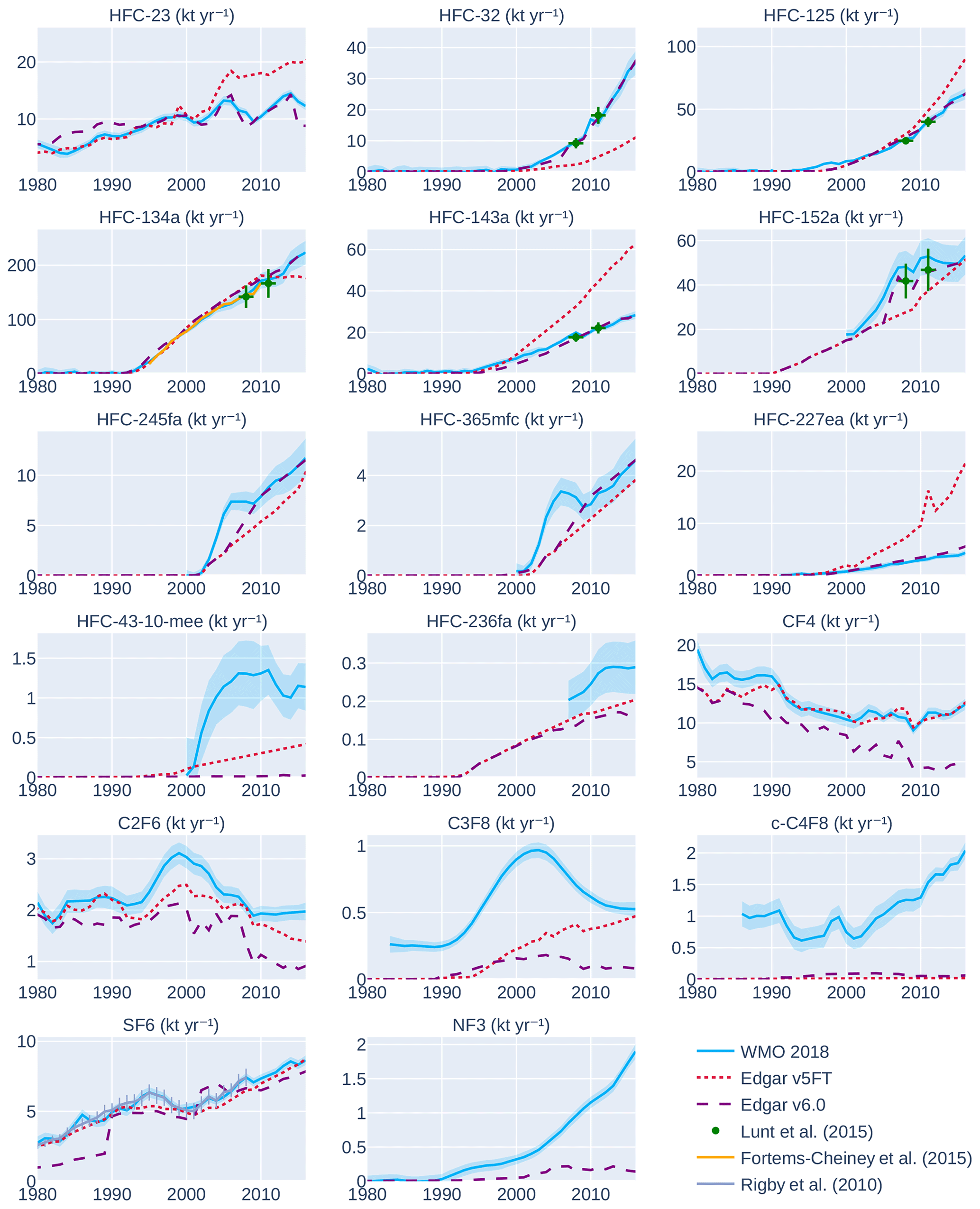
Figure 2 Comparison of top-down and bottom-up estimates for individual species of fluorinated gases in Olivier and Peters (2020) (EDGARv5FT) and EDGARv6 for 1980–2016. C₄F₁₀, C₅F₁₂, C₆F₁₄, and C₇F₁₆ are excluded. Top-down estimates from WMO 2018 (Engel and Rigby, 2018; Montzka and Velders, 2018) are shown as blue lines with blue shading, indicating 1σ uncertainties. Bottom-up estimates from EDGARv5 and EDGARv6 are shown in red dotted lines and purple dashed lines, respectively. Top-down estimates for some species are shown from Rigby et al. (2010), Lunt et al. (2015), and Fortems-Cheiney et al. (2015).

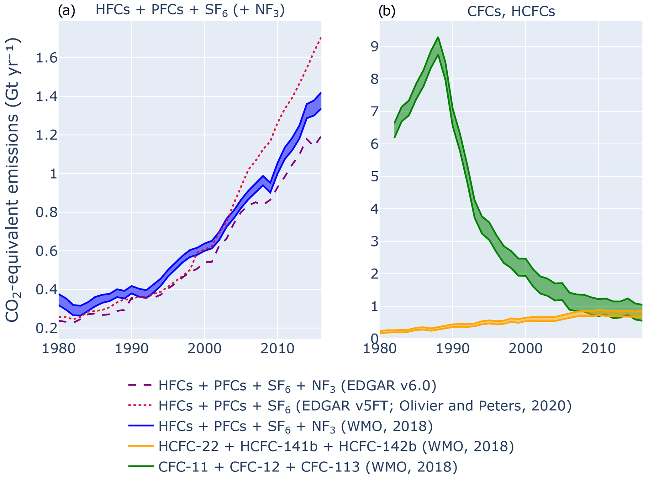
Figure 3 Comparison between top-down estimates and bottom-up EDGAR inventory data on GHG emissions for 1980–2016. (a) Total GWP-100-weighted emissions based on IPCC AR6 (Forster et al., 2021) of F-gases in Olivier and Peters (2020) (EDGARv5FT) (red dashed line, excluding C₄F₁₀, C₅F₁₂, C₆F₁₄, and C₇F₁₆) and EDGARv6 (purple dashed line) compared to top-down estimates based on AGAGE and NOAA data from WMO (2018) (blue lines; Engel and Rigby, 2018; Montzka and Velders, 2018). (b) Top-down aggregated emissions for the three most abundant CFCs (-11, -12, and -113) and HCFCs (-22, -141b, -142b) not covered in bottom-up emissions inventories are shown in green and orange. For top-down estimates the shaded areas between the two respective lines represent 1σ uncertainties.

The comparison of global top-down and bottom-up emissions for EDGARv6 and Olivier and Peters (2020) (EDGARv5FT) F-gas species (excluding heavy PFCs) is shown in Fig. 2 for the years 1980–2016 (or a subset thereof, depending on the availability of the top-down estimates). Where available, the various top-down estimates agree with each other within uncertainties. The magnitude of the difference between the WMO (2018) and EDGAR estimates varies markedly between species, years, and versions of EDGAR; for several HFCs, the top-down and bottom-up estimates often agree within uncertainties for EDGARv6 (but much less often in v5), whereas for c-C₄F₈, the top-down estimate is more than 100 times the EDGAR estimates. Some similarities and differences have been previously noted for earlier versions of EDGAR (Lunt et al., 2015; Mühle et al., 2010, 2019; Rigby et al., 2010). For SF₆, the relatively close agreement between EDGAR v4.0 and a top-down estimate has been discussed in Rigby et al. (2010). They estimated uncertainties in EDGAR v4.0 of ±10 % to ±15 %, depending on the year, and indeed, top-down values were consistent within these uncertainties. However, the agreement is now poorer during the 1980s in EDGARv6. For some PFCs (e.g. CF₄, C₂F₆), it was previously noted that some assumptions within EDGAR v4.0 had been validated against atmospheric observations, and hence EDGAR might be considered a hybrid of top-down and bottom-up methodologies for these species (Mühle et al., 2010). However, it is unclear for which other species similar validation has taken place or how these assumptions vary between versions of EDGAR.

When species are aggregated into F-gas total emissions, weighted by their current 100-year global warming potentials (GWPs) based on IPCC AR6 (Forster et al., 2021), we note that in Fig. 3a the Olivier and Peters (2020) (EDGARv5FT) estimates are around 10 % lower than the WMO 2018 values in the 1980s. Subsequently, EDGARv5FT estimates grow more rapidly than the top-down values and are almost 30 % higher than WMO 2018 by the 2010s. EDGARv6 emissions are around 10 % lower than the WMO 2018 values throughout. Given that detailed uncertainty estimates are not available for all EDGAR F-gas species, we base our uncertainty estimate solely on this comparison with the top-down values (see Fig. 3a) and therefore suggest a conservative uncertainty in aggregated F-gas emissions of ±30 % for a 90 % confidence interval. For individual species, the magnitude of this discrepancy can be orders of magnitude larger.

The F-gases in EDGAR exclude species such as CFCs and HCFCs, which are groups of substances regulated under the Montreal Protocol. Historically, total CO₂ eq. F-gas emissions have been dominated by the CFCs (Engel and Rigby, 2018). In particular, during the 1980s, peak annual emissions due to CFCs reached 9.1 ± 0.4 GtCO₂ eq. yr⁻¹ (Fig. 3), comparable to that of CH₄ and substantially larger than the 2018 emissions of the gases included in EDGARv5FT and EDGARv6 (1.3 GtCO₂ eq.) (Table 7). Subsequently, following the controls of the Montreal Protocol, emissions of CFCs declined substantially, while those of HCFCs and HFCs rose, such that CO₂ eq. emissions of the HFCs, HCFCs, and CFCs were approximately equal by 2016, with a smaller contribution from PFCs, SF₆, NF₃, and some more minor F-gases. Therefore, the GWP-weighted F-gas emissions in EDGAR, which are dominated by the HFCs, represent less than half of the overall CO₂ eq. F-gas emissions in 2016.

3.6 Aggregated GHG emissions

Based on our assessment of the relevant uncertainties above, we apply constant, relative uncertainty estimates for GHGs at a 90 % confidence interval that range from relatively low for CO₂ FFI (±8 %) to intermediate values for CH₄ and F-gases (±30 %) to higher values for N₂O (±60 %) and CO₂ from LULUCF (±70 %). To aggregate these and estimate uncertainties for total GHGs in terms of CO₂ eq. emissions, we are taking the square root of the squared sums of absolute uncertainties for individual (groups of) gases, using 100-year global warming potential (GWP-100) with values from IPCC AR6 (Forster et al., 2021, Sect. 7.6 and Supplement 7.SM.6 therein) to weight emissions of non-CO₂ gases but excluding uncertainties in the metric itself (see Sect. 3.7). Overall, this is broadly in line with IPCC AR5 (Blanco et al., 2014) but provides important adjustments in the evaluation of uncertainties of individual gases (CH₄, F-gases, CO₂-LULUCF) as well as the approach in reporting total uncertainties across GHGs.

3.7 GHG emissions metrics

GHG emissions metrics are necessary if emissions of non-CO₂ gases and CO₂ are to be aggregated into CO₂ eq. emissions. GWP-100 is the most common metric and has been adopted for emissions reporting under the transparency framework for the Paris Agreement (UNFCCC, 2019), but many alternative metrics exist in the scientific literature. The most appropriate choice of metric depends on the climate policy objective and the specific use of the metric to support that objective (i.e. why do we want to aggregate or compare emissions of different gases? What specific actions do we wish to inform?).

Different metric choices and time horizons can result in very different weightings of the emissions of short-lived climate forcers (SLCFs), such as CH₄. For example, 1 t CH₄ represents as much as 81 tCO₂ eq. if a global warming potential is used with a time horizon of 20 years or as little as 5.4 t CO₂ eq. if the global temperature change potential (GTP) is used with a time horizon of 100 years (Forster et al., 2021). More recent metric developments that compare emissions in new ways – e.g. the additional warming from sustained changes in SLCF emissions compared to pulse emissions of CO₂ – increase the range of metric values further and can even result in negative metric values for SLCFs if their emissions are falling rapidly (Allen et al., 2018; Cain et al., 2019; Collins et al., 2019; Lynch et al., 2020).

The contribution of SLCF emissions to total GHG emissions expressed in CO₂ eq. thus depends critically on the choice of GHG metric and its time horizon. However, even for a given choice, the metric value for each gas is also subject to uncertainties. For example, the GWP-100 for biogenic CH₄ has changed from 21 based on the IPCC Second Assessment Report (SAR) in 1995 to 28 or 34 based on IPCC AR5 (excluding or including climate–carbon cycle feedbacks) and to 27 based on IPCC AR6. These changes and remaining uncertainties arise from parametric uncertainties, differences in methodological choices, and changes in metric values over time due to changing background conditions.

Parametric uncertainties arise from uncertainties in climate sensitivity, radiative efficacy, and atmospheric lifetimes of CO₂ and non-CO₂ gases. IPCC AR6 assessed the parametric uncertainty of GWP for CH₄ as ±32 % and ±40 % for time horizons of 20 and 100 years, ±43 % and ±47 % for N₂O, and ±26–31 and ±33 %–38 % for various F-gases (Forster et al., 2021). The uncertainty of GTP-100 for CH₄ was estimated at ±83 %, which is larger than the uncertainty in a forcing-based metric due to uncertainties in climate responses to forcing (e.g. transient climate sensitivity).

Methodological choices introduce a different type of uncertainty, namely which indirect effects are included in the calculation of metric values and the strength of those feedbacks. For CH₄, indirect forcing caused by photochemical decay products (mainly tropospheric ozone and stratospheric water vapour) contributes almost 40 % of the total forcing from CH₄ emissions. More than half of the changes in GWP-100 values for CH₄ in successive IPCC assessments from 1995 to 2013 are due to re-evaluations of these indirect forcings. These uncertainties are incorporated into the above uncertainty estimates. In addition, warming due to the emission of non-CO₂ gases extends the lifetime of CO₂ already in the atmosphere through climate–carbon cycle feedbacks (Friedlingstein et al., 2013). Including these feedbacks results in higher metric values for all non-CO₂ gases, but the magnitude of this effect is uncertain; e.g. IPCC AR5 found the GWP-100 value for CH₄ without climate–carbon cycle feedbacks to be 28, whereas including this feedback would raise the value to between 31 and 34 (Gasser et al., 2016; Myhre et al., 2013; Sterner and Johansson, 2017). IPCC AR6 decided to include climate–carbon cycle feedbacks by default and no longer reports values without climate–carbon cycle feedbacks (Forster et al., 2021).

A third uncertainty arises from changes in metric values over time. Metric values depend on the radiative efficacy of CO₂ and non-CO₂ emissions, which in turn depend on the changing atmospheric background concentrations of those gases. Rising temperature can further affect the lifetime of some gases and hence their contribution to forcing over time for different emissions scenarios (Reisinger et al., 2011). Successive IPCC assessments take changing starting-year background conditions into account, which explains part of the changes in GWP-100 metric values in different reports. Applying a single metric value to a multi-decadal historical time series of emissions is therefore only an approximation of the correct metric value for any given emissions year, as e.g. the correct GWP-100 value for CH₄ emitted in the year 1970 will be different to the GWP-100 value for an emission in the year 2018. However, the literature does not offer a complete set of GWP-100 metric values for past concentrations and climate conditions covered in our time series.

Overall, we estimate the uncertainty in GWP-100 metric values, if applied to an extended historical emission time series, to be ±50 % for CH₄ and other SLCFs and ±40 % for non-CO₂ gases with longer atmospheric lifetimes (specifically, those with lifetimes longer than 20 years). If uncertainties in GHG metrics are considered and assumed independent for each gas (which may lead to an underestimate), the overall uncertainty of total GHG emissions in 2018 increases from ± 10 % to ±12 %. (However, in the following sections we do not include GWP uncertainties in our global, regional, or sectoral estimates.)

For the purpose of this paper, we use GWP-100 metric values from IPCC AR6 (Forster et al., 2021). As mentioned above, the most appropriate metric to aggregate GHG emissions depends on the objective. One such objective can be to understand the contribution of emissions in any given year to warming, while another can be to understand the contribution of cumulative emissions over an extended time period to additional warming relative to a given reference level. Sustained emissions of SLCFs such as CH₄ do not cause the same temperature response as sustained emissions of CO₂. Showing superimposed emissions trends of different gases over multiple decades using GWP-100 as an equivalence metric therefore does not necessarily represent the overall contribution to warming from each gas over that period. In Fig. 4 we therefore also show the modelled warming from emissions of each gas or group of gases – calculated using the simple climate model emulator FaIRv1.6.2 and calibrated to reproduce the pulse-response functions for each gas, consistent with IPCC AR6 (see Forster et al., 2021, their Supplement 7.SM.3). There are some differences compared to the contribution of each gas, based on GHG emissions expressed in CO₂ eq. using GWP-100 (see Fig. 8), in particular a greater contribution from CH₄ emissions to historical warming. This is consistent with warming from CH₄ being short-lived and hence having a more pronounced effect in the near term during a period of rising emissions. Nonetheless, Fig. 4 highlights that weighting emissions based on GWP-100 does not provide a vastly different overall story than modelled warming over the historical period when emissions of all gases have been rising, with CO₂ being the dominant and CH₄ being the second most important contributor to GHG-induced warming. Other metrics such as GWP* (Cain et al., 2019) offer an even closer resemblance between cumulative CO₂ eq. emissions and temperature change relative to a specified starting point, especially if SLCF emissions are no longer rising but potentially falling, as in mitigation scenarios.

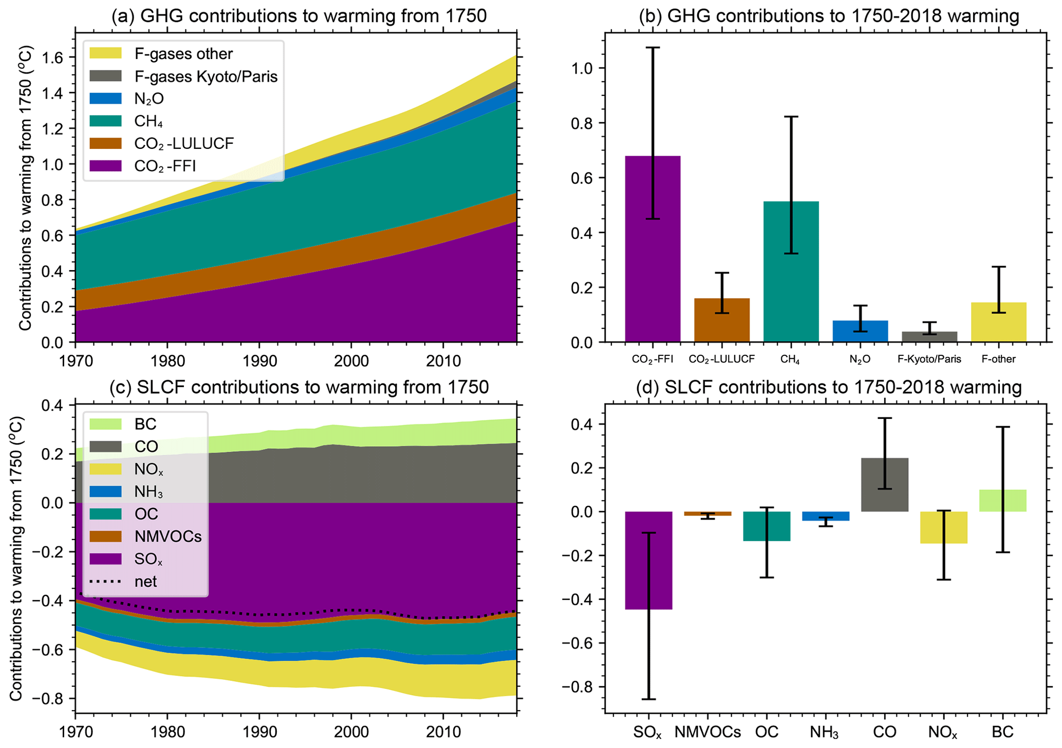
Figure 4 Contribution of different GHGs to global warming over the period 1750 to 2018. (a, b) Contributions from estimated with the FaIR reduced-complexity climate model. Major GHGs and aggregates of minor gases as a time series in (a) and as a total warming bar chart with 90 % confidence interval added in (b). (c, d) Contribution from short-lived climate forcers as a time series in (c) and as a total warming bar chart with the 90 % confidence interval added in (d). The dotted line in (c) gives the net temperature change from short-lived climate forcers. F-Kyoto/Paris includes the gases covered by the Kyoto Protocol and Paris Agreement as well as the HFCs, while F-other includes the gases covered by the Montreal Protocol but excluding the HFCs.

4 Results

Here we analyse global trends in anthropogenic GHG emissions in four time periods: (1) 1970–2018 to characterize the main trends in the data, (2) 2009–2018 to focus on the last decade, as well as (3) 2018 and (4) 2019 emissions levels.

4.1 Global anthropogenic GHG emissions for 1970–2018

There is high confidence that global GHG emissions have increased every decade from an average of 31 ± 4.3 GtCO₂ eq. yr⁻¹ for the decade of the 1970s to an average of 55 ± 5.9 GtCO₂ eq. yr⁻¹ during 2009–2018 as shown in Table 7. The decadal growth rate initially decreased from 1.8 % yr⁻¹ in the 1970s (1970–1979) to 0.9 % yr⁻¹ in the 1990s (1990–1999). After a period of accelerated growth during the 2000s (2000–2009) at 2.4 % yr⁻¹, triggered mainly by growth in CO₂-FFI emissions from rapid industrialization in China (Chang and Lahr, 2016; Minx et al., 2011), relative growth has decreased again to 1.2 % yr⁻¹ during the most recent decade (2009–2018). Uncertainties in aggregate GHG emissions have decreased over time as the share of less uncertain CO₂-FFI emissions estimates increased and the share of more uncertain emissions estimates such as CO₂-LULUCF or N₂O decreased.

Table 7 Average annual anthropogenic GHG emissions by decade and for selected individual years 1970–2018: CO₂ from fossil fuel combustion and industrial processes (FFI); CO₂ from land use, land-use change, and forestry (LULUCF); CH₄; N₂O; fluorinated gases (F-gases: HFCs, PFCs, SF₆, NF₃). Aggregate GHG emissions trends by groups of gases reported in GtCO₂ eq. converted based on global warming potentials with a 100-year time horizon (GWP-100) from IPCC AR6 (Forster et al., 2021). Uncertainties are reported for a 90 % confidence interval (see Sect. 3). Levels and growth are average values over the indicated time period. Additional Supplement tables show similar average annual GHG emissions by decade, also for major sectors (Table S2) and regions (Table S2).

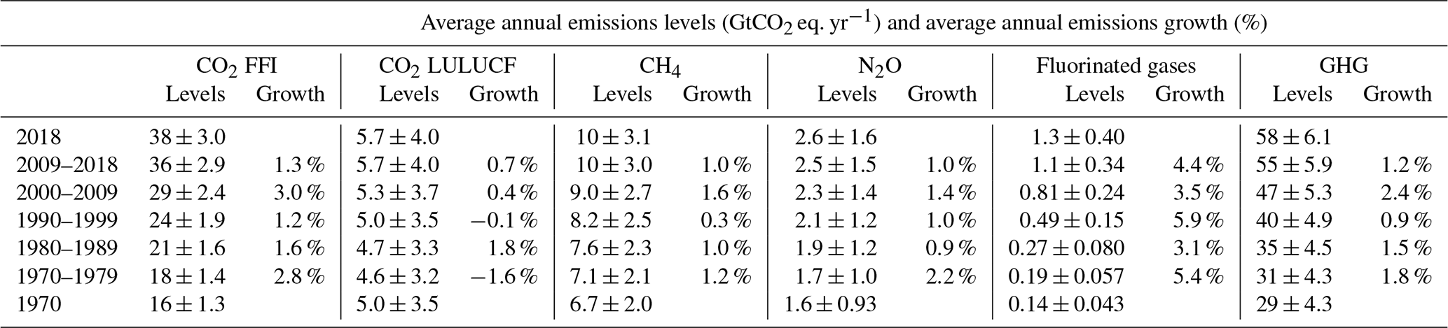
There is high confidence that emissions growth has been persistent but varied across different groups of gases. Decade-by-decade increases in global average annual emissions have been observed consistently across all (groups of) GHGs (Table 7). CO₂-LULUCF emissions have been more stable compared to other GHGs, albeit uncertain, and only recently started to show an upward trend. The pace and scale of emissions growth have varied across groups of gases. While average annual emissions of all GHGs together grew by about 75 % from 31 ± 4.3 GtCO₂ eq. yr⁻¹ during the 1970s (1970–1979) to 55 ± 5.9 GtCO₂ eq. yr⁻¹ during the most recent decade (2009–2018), CO₂-FFI emissions doubled from 18 ± 1.4 to 36 ± 2.9 GtCO₂ eq. yr⁻¹ and F-gases grew almost 5-fold from 0.19 ± 0.057 to 1.1 ± 0.34 GtCO₂ eq. yr⁻¹ across the same time period. In fact, persistent and fast growth in F-gas emissions has resulted in emissions levels that are now tracking at about 1.3 ± 0.40 GtCO₂ eq. yr⁻¹ in 2018 – 2.3 % of total GHG emissions measured as GWP-100. Relative increases in average annual emissions levels from the 1970s (1970–1979) to the most recent decade (2009–2018) were lower for CO₂-LULUCF (22 %; 1.0 GtCO₂ eq. yr⁻¹), CH₄ (41 %; 2.9 GtCO₂ eq. yr⁻¹) and N₂O (49 %; 0.83 GtCO₂ eq. yr⁻¹) (see Table 7). In absolute terms, CO₂ dominated increases in GHG emissions since the 1970s, followed by CH₄. However, there is low confidence that the reported increases in CO₂-LULUCF emissions by decade actually constitute a statistically robust trend given the large uncertainties involved. In fact, two bookkeeping models underlying the CO₂-LULUCF data show opposing positive and negative trends (BLUE and H&N, respectively), while the third model (OSCAR), averaging over simulations that use either the same land-use forcing as BLUE (LUH2) or H&N (FAO/FRA), tracks the approximate mean of these (see also Sect. 3.2). Dynamic global vegetation models, which also use the LUH2 forcing, show higher estimates recently, explained by them considering the loss in sink capacity while the bookkeeping models do not (see Fig. 1). Overall, the different lines of evidence are inconclusive with regard to an upward trend in CO₂-LULUCF emissions.

Global anthropogenic GHG emissions grew continuously slower than world gross domestic product (GDP) across all (groups of) individual gases, resulting in a sustained decline in the GHG intensity of GDP as shown in Fig. 5. The only exception is the group of F-gases, for which the GHG intensity of GDP has significantly increased since 1970, with a marked acceleration during the 1990s and the early 2000s, an intermediate drop in the late 2000s, and continued growth thereafter. Per capita GHG emissions have been fluctuating substantially, with a sustained decline in global per capita GHG emissions since the 1970s followed by an approximate 15-year period of continued growth from the 2000s. In recent years, per capita GHG emissions levels have stabilized without clear evidence for peaking. For CO₂-FFI emissions, sustained growth in per capita emissions can be observed since the mid-1990s, levelling off during the last decade. Per capita emissions for CO₂-LULUCF, CH₄, and N₂O declined consistently since the 1970s, but this trend has flattened out since the mid-1990s or early 2000s. Per-capita F-gas emissions show sustained and rapid growth over the full time period, interrupted only by a small decline in the late 2000s.

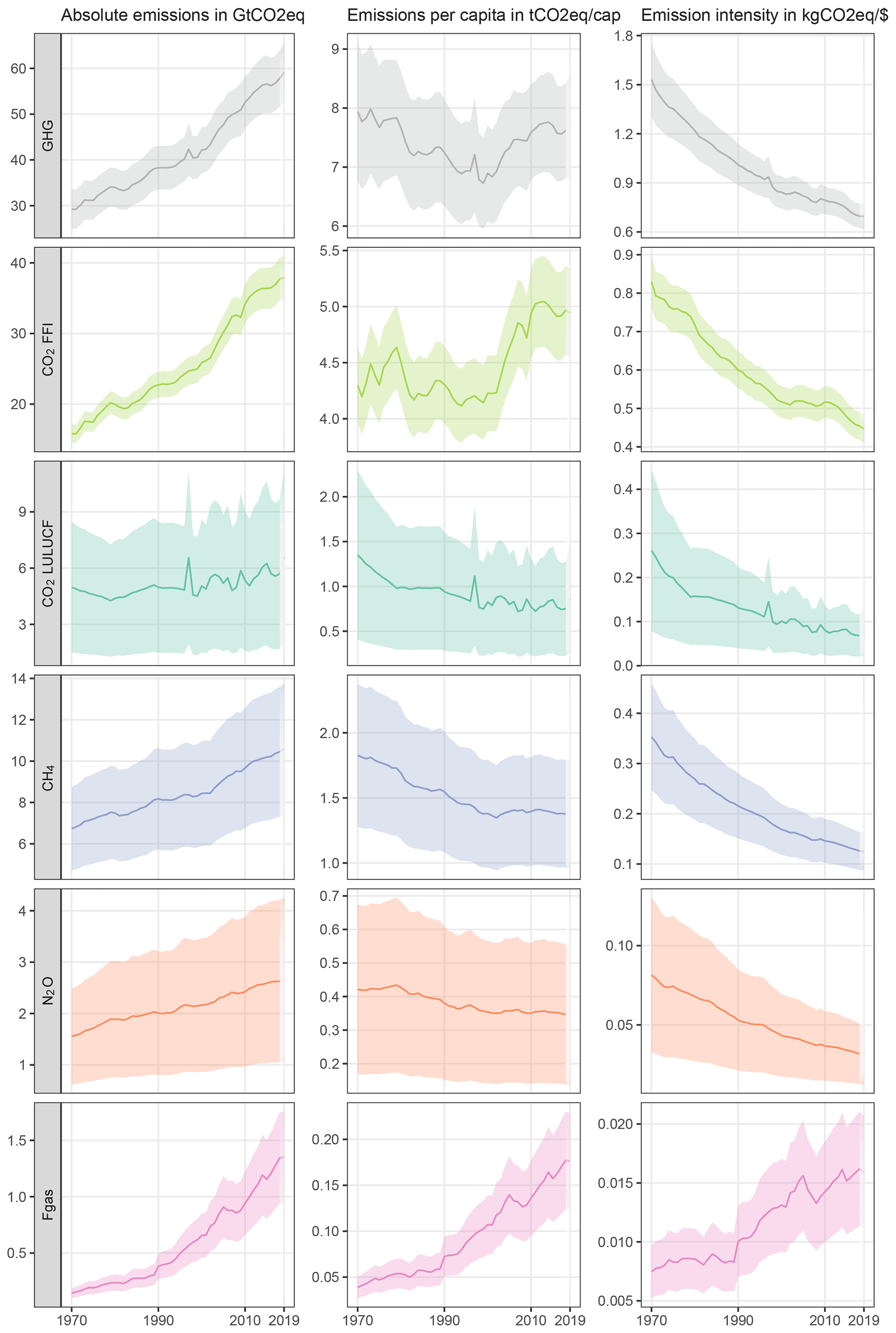
Figure 5 Global GHG emissions trends for 1970–2019 by individual (groups of) gases and in aggregate: GHGs (black); CO₂-FFI (light green); CO₂-LULUCF (dark green); CH₄ (blue); N₂O (orange); fluorinated gases (pink). Aggregate GHG emissions trends by groups of gases reported in GtCO₂ eq. converted based on global warming potentials with a 100-year time horizon (GWP-100) from IPCC AR6 (Forster et al., 2021). Coloured shadings show the associated uncertainties at a 90 % confidence interval without considering uncertainties in GDP and population data (see below). The first column shows emissions trends in absolute levels (GtCO₂ eq. yr⁻¹). The second column shows per capita emissions trends (tCO₂ eq./cap) using UN population data for normalization (World Bank, 2021). The third column shows emissions trends per unit of GDP (kgCO₂ eq./USD) using GDP data in constant USD 2010 from the World Bank for normalization (World Bank, 2021).

The continuous increase in global anthropogenic GHG emissions since the 1970s was mainly driven by activity growth in three major sectors: energy supply, industry, and transportation (see Table S2, Fig. S4). In energy supply and transportation, average annual emissions were about 2.3 and 2.2 times larger for 2009–2018 than for 1970–1979, respectively, growing from 8.4 to 19 GtCO₂ eq. yr⁻¹ and from 3.6 to 8.0 GtCO₂ eq. yr⁻¹, respectively. In industry, average annual GHG emissions were 1.8 times larger, growing from 7.3 GtCO₂ eq. yr⁻¹ in 1970–1979 to 13 GtCO₂ eq. yr⁻¹ in 2009–2018. At the sub-sector level, electricity and heat and road transport are the largest segments, growing 2.9 and 2.6 times between 1970 and 1979 and between 2009 and 2018, respectively, from an average of 4.6 to 13 GtCO₂ eq. yr⁻¹ and 2.2 to 5.7 GtCO₂ eq. yr⁻¹. The fastest-growing sub-sector has been process emissions from cement, which is 4.1 times larger in 2009–2018 compared to 1970–1979 and currently accounts for an average of 1.4 GtCO₂ eq. yr⁻¹. Other rapidly expanding sectors are international aviation (2.8 times larger on 1970–1979 levels), chemicals (1.9 times larger), metals (1.7 times larger), and waste (1.7 times larger). Growth in GHG emissions in AFOLU and buildings has been much more moderate, with average annual GHG emissions only about 26 % and 10 % higher for 2009–2018 than for 1970–1979.

Most GHG emissions growth occurred in Asia and the Developing Pacific as well as the Middle East, where emissions more than tripled from 6.3 and 0.8 GtCO₂ eq. yr⁻¹ in 1970–1979 to 23 and 2.8 GtCO₂ eq. yr⁻¹ in 2009–2018, respectively (see Table S1). Over the same time period GHG emissions grew 2.2 times in Africa and 1.7 times in Latin America and the Caribbean, while average annual anthropogenic GHG emissions levels in developed countries and eastern Europe and western–central Asia remained stable. However, Fig. 6 highlights important variability at the country level. Note that these country-level estimates exclude CO₂-LULUCF emissions, because we assign low confidence to them. First, GHG emissions growth is taking place against the background of large differences in per capita GHG emissions between and within regions. For example, GHG emissions in developed countries have stabilized at high levels of per capita emissions compared to most other regions. Similarly, some countries in the Middle East are among the largest GHG emitters in per capita terms, while other countries of the region such as Yemen have seen comparatively little economic development, showing low levels of per capita emissions. Second, the growth in GHG emissions has also been highly varied. For example, several developed countries in Europe such as the UK, Germany, or France have lower GHG emissions levels today than in the 1970s. In other countries like the USA GHG emissions levels are still considerably higher today even though they have recently started reducing GHG emissions – unlike Australia or Canada, which have until now only begun stabilizing their GHG emissions levels. A comprehensive assessment of country progress in reducing GHG emissions can be found in Lamb et al. (2021b).

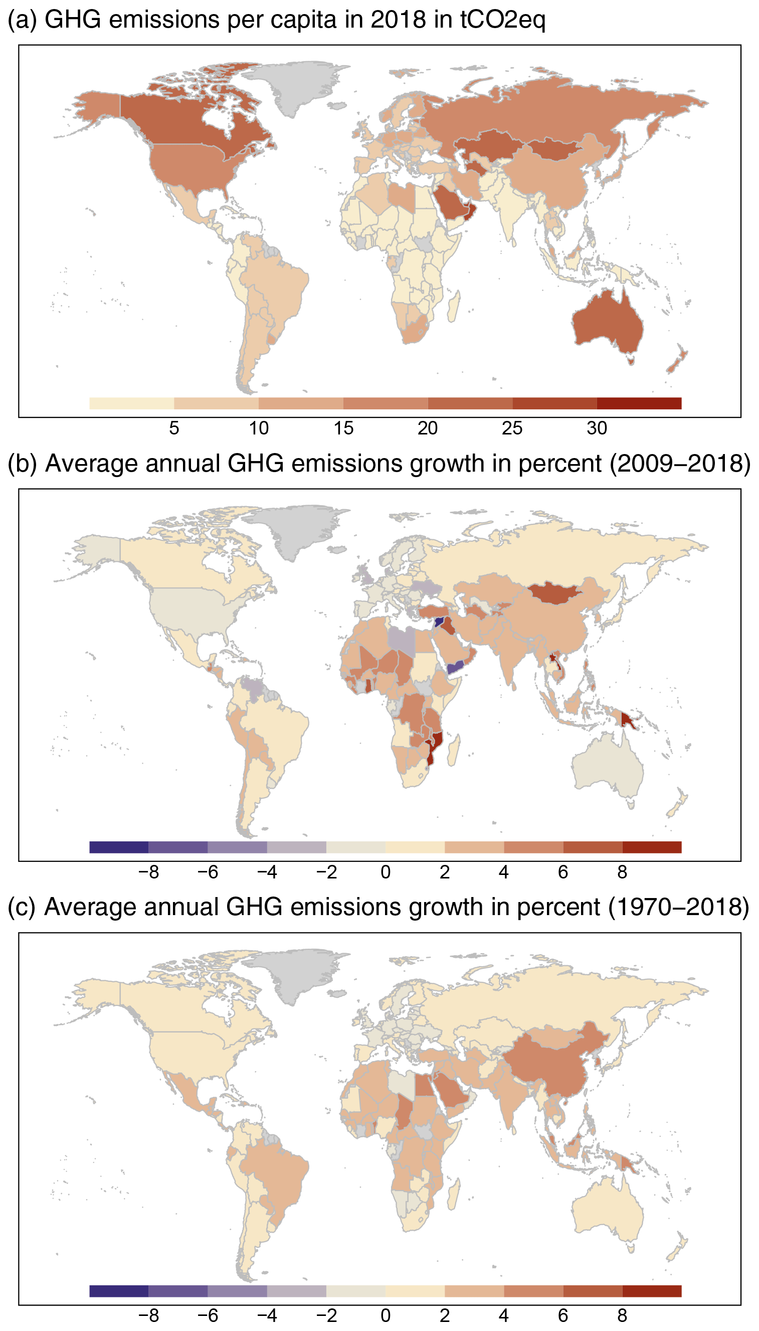
Figure 6 Levels of and changes in GHG emissions by country. Aggregate GHG emissions are reported in GtCO₂ eq. based on global warming potentials with a 100-year time horizon (GWP-100) from IPCC AR6 (Forster et al., 2021). Panel (a) shows per capita GHG emissions levels (tCO₂ eq. yr⁻¹) for the year 2018 using UN population data for normalization (World Bank, 2021). Panel (b) shows average annual changes (in %) in GHG emissions by countries for 2009–2018. Panel (c) shows average annual changes (in %) in GHG emissions by countries for 1970–2018. Note that this excludes CO₂-LULUCF, as there is currently low confidence in national-level estimates.

In Fig. 7 we compare historic GHG emissions trends with different scenarios to explore how emissions are developing relative to the range of projected future outcomes. The Integrated Assessment Modelling (IAM) community quantified five shared socioeconomic pathways (SSPs) for different levels of radiative forcing in 2100 using six different IAMs (Riahi et al., 2017; Rogelj et al., 2018). The SSPs are grouped according to their radiative forcing ranging from 1.9 to 8.5 W m⁻², aimed at spanning the full range of potential outcomes. The Coupled Model Intercomparison Project Phase 6 (CMIP6) (Eyring et al., 2016) took a subset of these quantified SSPs as the basis for future climate projections (Gidden et al., 2019; O'Neill et al., 2016). In recent years, the use of the very high forcing scenarios – particularly SSP5-8.5 – has been debated in the scientific community (e.g. Hausfather and Peters, 2020b, a; Pedersen et al., 2020; Schwalm et al., 2020).

Historical GHG emissions from our database are consistent with the levels and trends in the scenario data, despite the scenarios being calibrated on older data sources (Gidden et al., 2019) – mainly CEDS (Hoesly et al., 2018). The observed differences are larger for the GHGs with the highest uncertainty, notably CO₂-LULUCF, N₂O, and F-gas emissions (Sect. 3.2, 3.4, and 3.5). Across the different GHGs, historical emissions track on aggregate with the higher forcing scenarios such as the SSP3-7.0 and SSP5-8.5 markers, in terms of both levels and growth rates. CO₂-FFI emissions still tend towards the higher end of the scenario range shown here, but there are signs that CO₂-FFI emissions are slowing to more moderate forcing levels (e.g. SSP4-6.0 and SSP2-4.5) when considering recent trends (Hausfather and Peters, 2020a). CH₄ and N₂O emissions sit more in the middle and at the lower end of the scenario range – the latter driven by the lower levels of N₂O emissions in EDGAR – and F-gases are consistent with the scenarios. Total GHG emissions track the higher-end scenarios.

Figure 7 highlights the very different future emission trajectories envisioned by IAMs for individual gases – particularly at radiative forcing levels that are consistent with the goal of the Paris Agreement such as SSP1-2.6 and SSP1-1.9. In contrast to CO₂ emission, non-CO₂ forcers such as anthropogenic CH₄ and N₂O emissions are not reduced to zero. However, in many scenarios, F-gases reach zero emissions. N₂O emissions remain at similar levels to today in some of the scenarios, with a 1.9 W m⁻² forcing at the end of the century, while they are about halved in others. Reductions in CH₄ emissions are a bit more pronounced, ranging from about 100 to 200 MtCH₄ yr⁻¹ in 2100 compared to almost 400 MtCH₄ yr⁻¹ in 2019. CO₂-LULUCF emission trajectories overlap for different forcing levels, partly reflecting the complexities of modelling land-use change, but overall show a tendency towards a net carbon sink even in SSPs with little or even without climate policy. Given recent trends in land-use change emissions, it could be questioned whether the scenarios adequately explore the uncertainty in future land-use change emissions (Hausfather and Peters, 2020b).

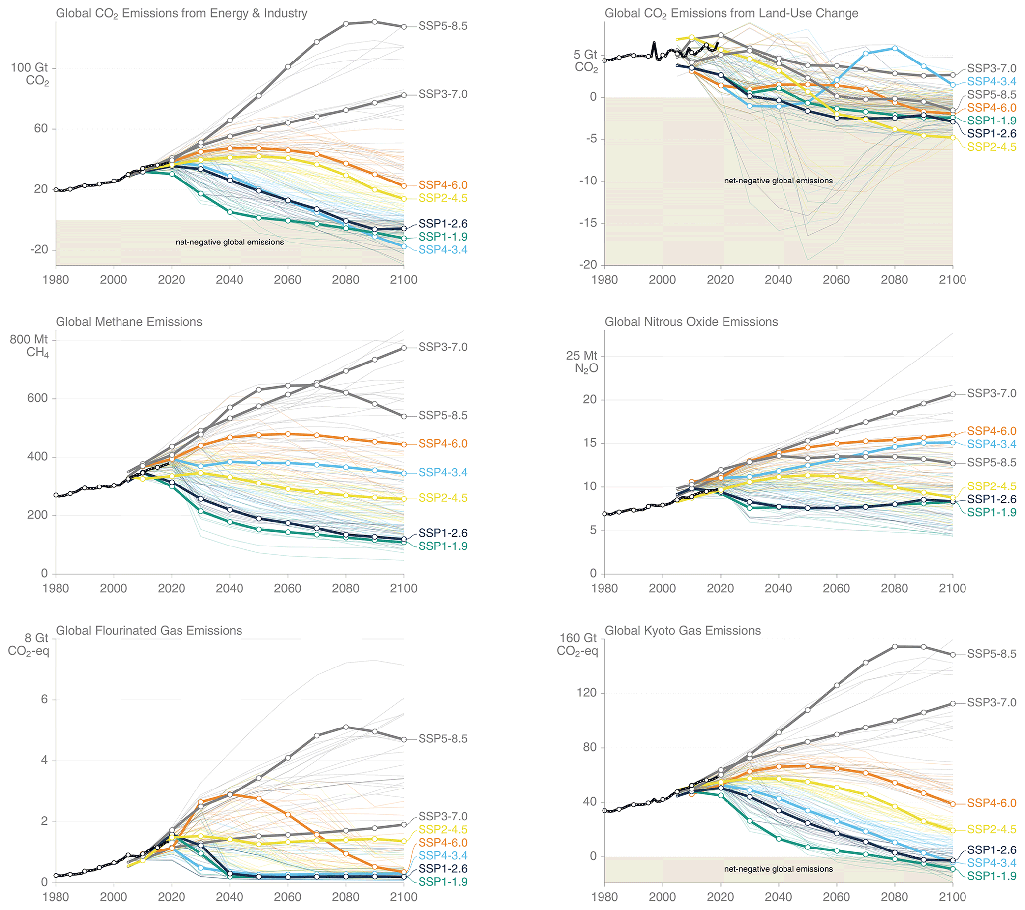
Figure 7 Historical emissions of GHGs and future projections in socio-economic scenarios. The historical emissions are from this dataset. GHG emissions are reported in GtCO₂ eq. converted based on global warming potentials with a 100-year time horizon (GWP-100) from IPCC AR6 (Forster et al., 2021). The Shared Socioeconomic Pathways (SSPs) are from the SSP database version 2 (Riahi et al., 2017; Rogelj et al., 2018). See also https://tntcat.iiasa.ac.at/SspDb/ (last access: 3 November 2021). Highlighted scenarios are the markers used in CMIP6 (O'Neill et al., 2016) after harmonization (Gidden et al., 2019).

4.2 Global GHG emissions for the last decade 2009–2018

There is high confidence that global anthropogenic GHG emissions levels were higher in 2009–2018 than in any previous decade and that GHG emissions levels have grown across the most recent decade. Average annual GHG emissions for 2009–2018 were 55 ± 5.9 GtCO₂ eq. yr⁻¹ compared to 47 ± 5.3 and 40 ± 4.9 GtCO₂ eq. yr⁻¹ for 2000–2009 and 1990–1999, respectively. This marks an increase of about 8.3 GtCO₂ eq. yr⁻¹ or 18 % between the two most recent decades, 2000–2009 and 2009–2018. While average annual GHG emissions slowed from 2.4 % in 2000–2009 to 1.2 % in 2009–2018, the absolute increase in GHG emissions from one decade to the next has never been larger since the 1970s, as covered by the data here, and within all human history, as suggested by available long-term data (e.g. Friedlingstein et al., 2020; Hoesly et al., 2018). The largest contributor to this increase was a growth in annual CO₂-FFI emissions of about 6.3 Gt yr⁻¹ decade on decade, complemented by increases of 1.1 GtCO₂ eq. yr⁻¹ in CH₄ emissions, 0.36 Gt yr⁻¹ in CO₂-LULUCF emissions, 0.25 GtCO₂ eq. yr⁻¹ in N₂O emissions, and 0.31 GtCO₂ eq. yr⁻¹ in F-gas emissions.

More than half of the recent growth in global GHG emissions between 2009 and 2018 came from China (3.1 GtCO₂ eq. yr⁻¹) and India (0.95 GtCO₂ eq. yr⁻¹) (Fig. 8). Among the major emitters, the fastest GHG emissions growth was observed for Turkey, with average annual rates of 4.2 % yr⁻¹ between 2009 and 2018, followed by Indonesia (3.8 % yr⁻¹), Saudi Arabia (3.4 % yr⁻¹), India (3.2 % yr⁻¹), Pakistan (3.1 % yr⁻¹), and China (2.2 % yr⁻¹). GHG emissions reductions achieved by countries over the last decade are comparatively small even though there is a growing number of countries on sustained emissions reductions trajectories (Lamb et al., 2021b; Le Quéré et al., 2019b). The USA showed the largest net anthropogenic GHG emissions reductions of 0.14 GtCO₂ eq. yr⁻¹ between 2009 and 2018, resulting from reductions of about the same size in CO₂ emissions – mainly from a switch from coal to gas in the context of the shale gas expansion. Other countries with decreasing GHG emissions levels were Australia (−0.01 GtCO₂ eq. yr⁻¹), Germany (−0.02 GtCO₂ eq. yr⁻¹), and the United Kingdom (−0.12 GtCO₂ eq. yr⁻¹), where the latter shows the fastest average annual reductions in relative terms at a rate of 2.9 % yr⁻¹ in the sample (Fig. 8) – in line with some GHG emissions reduction scenarios that limit global warming to well below 2 ^∘C (Lamb et al., 2021b). Further information on country contributions to GHG emissions changes since 1990s – an important reference for UN climate policy – is shown in Supplement Fig. S3.

Official statistics submitted annually by Annex I countries of the Kyoto Protocol (see Fig. 9) to the UNFCCC (UNFCCC-CRFs) indicate 0.9 % lower emissions over the period 1990–2018 (excluding CO₂-LULUCF emissions) (UNFCCC, 2021, accessed through Gütschow et al., 2021a). The vast majority of the Annex I countries, which contributed 33 % of the global GHG emissions in 2018 (according to the dataset presented in this paper), report lower total GHG emissions in 2018 as compared with the data presented here. The total emissions of the Annex I countries in 2018 stand at 17.2 GtCO₂ eq. yr⁻¹ according to the national inventories, 1.2 % lower than the data presented here for the same countries. Both datasets, however, agree in terms of the average annual growth rates over the last decade (2009–2018), which stood at −0.4 % for the total GHG emissions of the Annex I countries. For single countries there is still some divergence in growth rates observed between the national inventories and the dataset presented here (Fig. 8b and c). Additional analysis comparing our data with UNFCCC-CRF inventories for individual (groups of) gases and countries is provided in Supplement Figs. S3 and S4.

Sectoral GHG emissions were either stable or increased between 2009 and 2018. There is high confidence that no substantive GHG emissions reductions were observable for entire sectors at the global level. The most substantial growth was observed in the metal industry, with an average annual growth rate of 3.4 % yr⁻¹ between 2009 and 2018 followed by the chemical industry (2.5 % yr⁻¹), road transport (2.0 % yr⁻¹), electricity and heat (1.9 % yr⁻¹), and the cement industry (1.7 % yr⁻¹) (Fig. 8d–e). International and domestic aviation, which is small in its contribution to global GHG emissions (and is therefore not shown in Fig. 8e–f), exhibits even larger growth rates of 3.8 % yr⁻¹ (0.69 GtCO₂ eq. yr⁻¹) and 3.7 % yr⁻¹ (0.39 GtCO₂ eq. yr⁻¹), respectively.

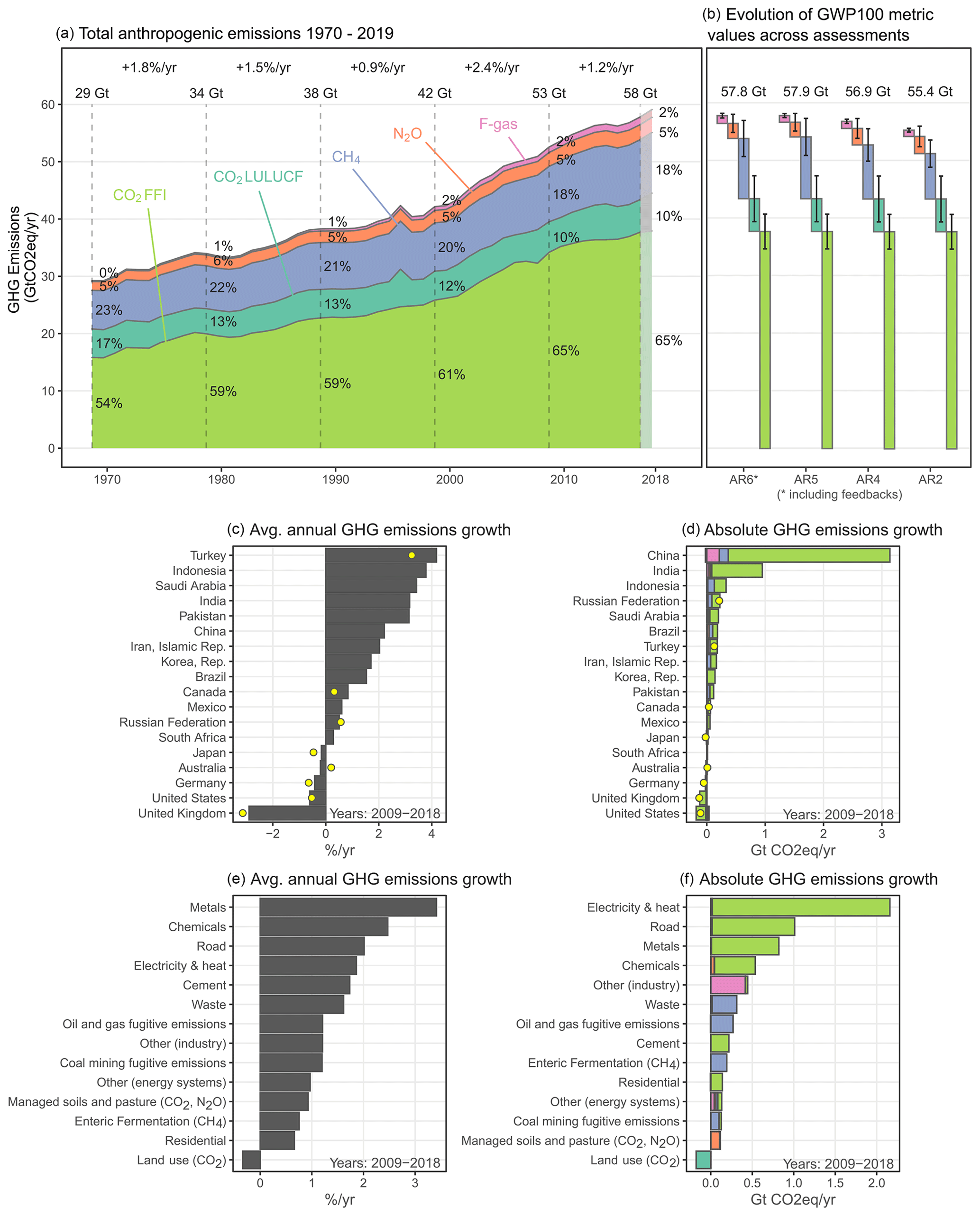
Figure 8 Total anthropogenic GHG emissions (Gt CO₂ eq. yr⁻¹) for 1970–2018 and initial estimates for 2019 as well as country and sector contributions to changes over the last decade (2009–2018): CO₂-FFI (light green); CO₂-LULUCF (dark green); CH₄ (blue); N₂O (orange); fluorinated gases (pink); all GHGs (black). Gases are reported in GtCO₂ eq. converted based on global warming potentials with a 100-year time horizon (GWP-100) from IPCC AR6 (Forster et al., 2021). (a) Aggregate GHG emissions trends for 1970–2018 with the initial 2019 estimate. Average annual growth rates by decade are reported at the top of the figure (in % yr⁻¹). Transparent colour for the 2019 estimate indicates its preliminary nature and lower confidence associated with it. (b) Waterfall diagrams juxtapose GHG emissions for 2018 in CO₂ eq. units using GWP-100 values from the IPCC's AR6, AR5, AR4, and AR2, respectively. Error bars show the associated uncertainties at a 90 % confidence interval (see Sect. 3). Panels (c) and (d) show relative (in % yr⁻¹) and absolute (in GtCO₂ eq. yr⁻¹) average annual changes in GHG emissions for a selection of the largest emitting countries (contributing 75 % of global GHG emissions in 2018), excluding CO₂-LULUCF emissions as uncertainties in our estimates are too high for country-level reporting. The yellow dots represent the emissions data from UNFCCC-CRFs  (2021) that were accessed through Gütschow et al. (2021a). Further comparisons with CRF data are provided in Figs. S3 and S4. Panels (e) and (f) show relative (in % yr⁻¹) and absolute (in GtCO₂ eq. yr⁻¹) changes in GHG emissions for a selection of the largest emitting sectors (see Table 2) (contributing 90 % of global GHG emissions in 2018).

4.3 Global GHG emissions in 2018

Global net anthropogenic GHG emissions continued to grow and reached 58 ± 6.1 GtCO₂ eq. in 2018 (Fig. 8). In 2018, CO₂ emissions from FFI were 38 ± 3.0 Gt, CO₂ from LULUCF 5.7 ± 4.0 Gt, CH₄ 10 ± 3.1 GtCO₂ eq., N₂O 2.6 ± 1.6 GtCO₂ eq. and F-gases 1.3 ± 0.40 GtCO₂ eq. Of the 58 ± 6.1 GtCO₂ eq. emissions in 2018, 35 % (20 GtCO₂ eq. yr⁻¹) were from energy supply, 24 % (14 GtCO₂ eq. yr⁻¹) from industry, 21 % (12 GtCO₂ eq. yr⁻¹) from AFOLU, 15 % (8.6 GtCO₂ eq. yr⁻¹) from transport, and 5.6 % (3.3 GtCO₂ eq. yr⁻¹) from buildings. In 2018, the largest absolute contributions in GHG emissions were from Asia and the developing Pacific (43 %), developed countries (25 %), and Latin America and the Caribbean (10 %). China (14 GtCO₂ eq. yr⁻¹), the USA (6.4 GtCO₂ eq. yr⁻¹), India (3.7 GtCO₂ eq. yr⁻¹), and the Russian Federation (2.4 GtCO₂ eq. yr⁻¹) remained the largest country contributors to global GHG emissions, excluding CO₂-LULUCF, as we do have not sufficient confidence to report these data at the country level.

In 2018, emissions were 1.0 GtCO₂ eq. or 1.8 % higher than the 57 ± 6.9 GtCO₂ eq. in 2017. Most of this growth (0.78 Gt yr⁻¹, 2.1 % yr⁻¹) was related to increases in CO₂-FFI emissions. Also, F-gas emissions (0.067 GtCO₂ eq. yr⁻¹, 5.2 % yr⁻¹) and CO₂-LULUCF emissions (0.12 Gt yr⁻¹, 2.1 % yr⁻¹) increased significantly, but we assign low confidence to the magnitude of the growth, particularly for CO₂-LULUCF due to the high uncertainties attached. Emissions in CH₄ and N₂O were rather stable between 2017 and 2018, with growth rates of 0.8 % yr⁻¹ and 0.0 % yr⁻¹, respectively. Given the prevailing uncertainties, there is low confidence that GHG emissions have never been higher than in 2018 as suggested by the data but high confidence that average annual GHG emissions have never been higher for a decade than in 2009–2018 (see Friedlingstein et al., 2020; Hoesly et al., 2018).

4.4 Fast-track estimates for GHG emissions in 2019

GHG emissions in 2019 are estimated at 59 ± 6.6 GtCO₂ eq. yr⁻¹. This is 2.2 % (1.3 GtCO₂ eq. yr⁻¹) higher than emissions in 2018 and an increase in the annual growth rate compared to 2017–2018 of 1.8 % (1.0 GtCO₂ eq.). These estimates are in large part derived from less complete information, and there is less confidence in the exact magnitude. The magnitude of the recent emissions growth is particularly uncertain, because a large portion of emissions growth between 2018 and 2019 (0.91 Gt yr⁻¹, 16.1 % yr⁻¹) is related to increases in very uncertain CO₂-LULUCF emissions estimates. All three bookkeeping models show a consistent trend of increasing emissions in 2019, culminating in an average estimate for net anthropogenic CO₂-LULUCF emissions of 6.6 ± 4.6 Gt yr⁻¹. This was due to a surge of fire emissions from peat burning, deforestation, and degradation, occurring mainly in equatorial Asia and the Amazon and substantially exceeding average rates in the previous decade (Friedlingstein 2020; GFED4.1s; van der Werf et al., 2017). Anthropogenic fire processes are not captured well by the underlying land-use datasets. Further, the 2019 estimate was extrapolated for all three bookkeeping estimates by applying additional information on emissions from equatorial Asia peat fires and tropical deforestation and degradation fires (GFED4.1s; van der Werf et al., 2017) in a similar way (Friedlingstein et al., 2020). This explains the consistent upward trend for all three bookkeeping estimates for 2019.

Non-LULUCF CO₂ sources contributed relatively little to the 2019 increase in emissions. CO₂-FFI emissions were relatively stable (0.20 GtCO₂ eq. yr⁻¹, 0.5 % yr⁻¹), as were F-gases (0.4 % yr⁻¹), while N₂O and CH₄ emissions increased with growth rates of 1.2 % and 1.1 %, respectively. In terms of regions, 89 % (1.1 GtCO₂ eq. yr⁻¹) of the emissions growth in 2019 occurred in Asia and the Developing Pacific, followed by Latin America (0.30 GtCO₂ eq. yr⁻¹, 24.1 %) and international shipping and aviation (0.078 GtCO₂ eq. yr⁻¹, 6.2 %).

5 Data availability

The emissions dataset used for this study (Minx et al., 2021) is available at https://doi.org/10.5281/zenodo.5566761.

6 Discussion

In this article we provide a comprehensive, synthetic, and detailed dataset for global, regional, national, and sectoral GHG emissions from anthropogenic activities covering the last 5 decades (1970–2019). This is based on the EDGARv6 GHG emissions inventory but additionally includes a fast-track update to 2019 for non-CO₂ emissions and data on CO₂-LULUCF emissions from three global bookkeeping models. We assess uncertainties in our estimates by combining statistical analysis of the underlying data and expert judgement based on an in-depth review of the literature by each gas. We report uncertainties at a 90 % confidence interval (5th–95th percentile range). We note that national emissions inventory submissions reported to the UNFCCC are requested to report uncertainty using a 95 % (2σ) confidence interval. The use of this broader uncertainty interval implies, however, a relatively high degree of knowledge about the uncertainty structure of the associated data, which is not present over the emission sectors and species considered here.

Our uncertainty assessment is broadly consistent with previous assessments focussing on all GHGs (Blanco et al., 2014; UNEP, 2020), but we provide some important updates. Our evidence-informed uncertainty judgements are higher for CO₂-LULUCF (±70 % rather than ± 50 %) and CH₄ (±30 % rather than ±20 %), drawing from the Global Carbon Budget (Friedlingstein et al., 2020), the Global Methane Budget (Saunois et al., 2020), and the available literature (e.g. Janssens-Maenhout et al., 2019; Solazzo et al., 2021). We note the limited literature on the uncertainties in F-gas emissions in global emissions inventories and recognize the divergence between bottom-up inventory estimates and top-down atmospheric measurements for individual F-gases. Our revised uncertainty estimate for aggregate F-gas emissions of ±30 % (rather than ±20 %) reflects the smaller aggregate deviation observed for aggregate F-gas emissions across species. We further acknowledge that we apply the same uncertainty estimates to our fast-track extension to 2019 even though the 2019 estimates themselves will be more uncertain. However, our analysis almost exclusively focusses on the data up to 2018 that are based on full data releases, where our global uncertainty estimates are applied.

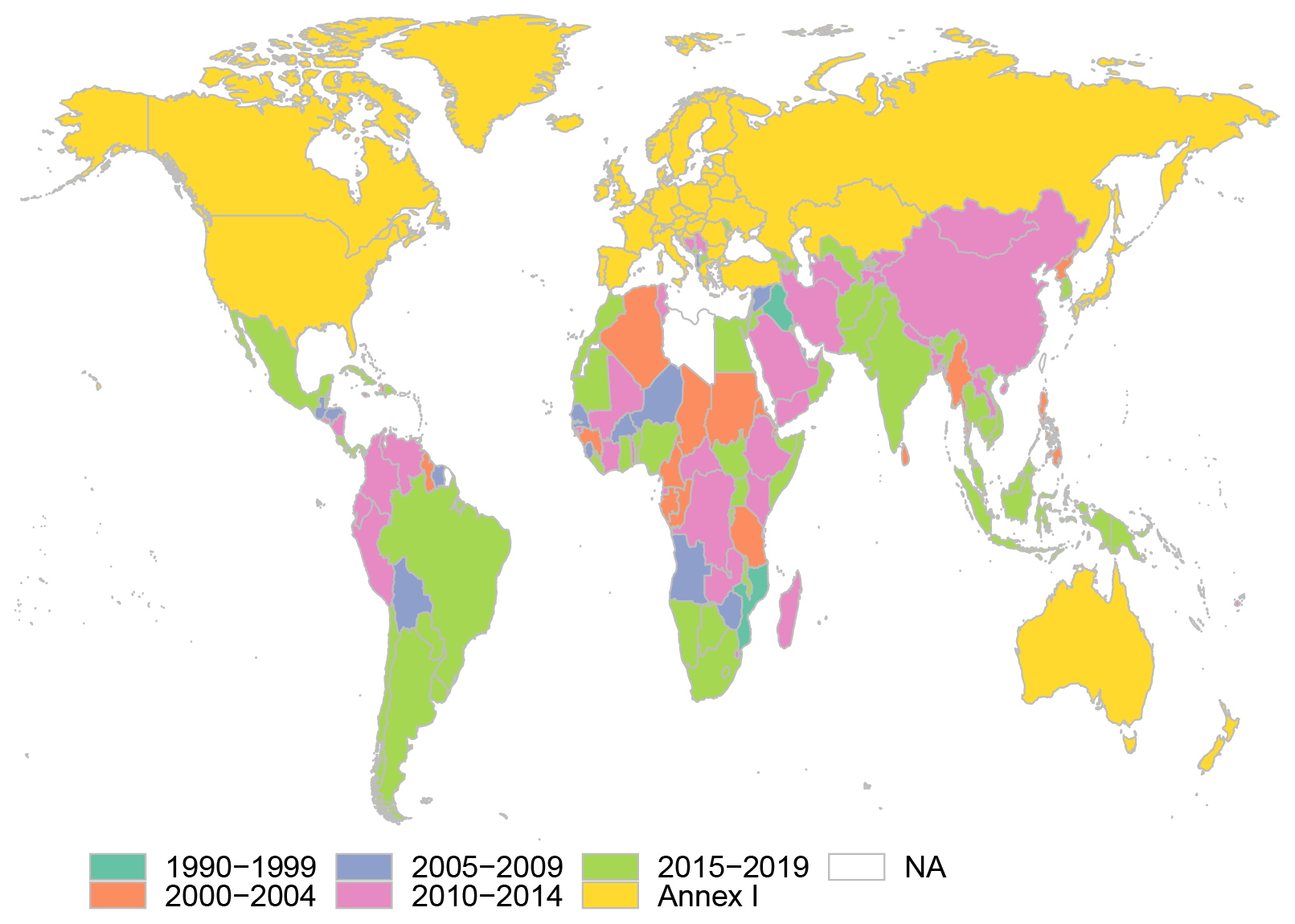
Figure 9 Overview of the most recent GHG emissions inventories submitted to the UNFCCC: the map captures the last year for which emission inventories were conducted and published by the UNFCCC on their website (as of 28 September 2021), including CRFs, BURs, and NCs. Annex I countries, according to the UNFCCC definition, have reported their last inventories for 2019 (UNFCCC, 2021). Updated from Janssens-Maenhout et al. (2019).

Our analysis involves aggregating GHG emissions into a single unit using GWP-100 values from IPCC AR6. By doing so we follow the practice taken in UNFCCC inventory reporting and large parts of the literature on climate change mitigation. However, we recognize intense scientific and academic debates about the aggregation of GHGs into a single unit and alternative choices of metrics (Forster et al., 2021) (see Sect. 3.7). We therefore also use a simple climate model to assess the warming contribution by the individual groups of gases and find that for the historical period when emissions are growing, the GWP-100 gives a reasonable approximation to the warming contributions, but this is not expected to hold when emissions change trajectory under mitigation. In the absence of a comprehensive uncertainty analysis that covers CO₂-LULUCF as well as F-gas emissions, we estimate the overall uncertainty of aggregated GHG emissions by simply adding the individual uncertainties judgements by (groups of) gases in quadrature under the assumption of their independence. Over time, uncertainties fluctuate between 10 % and 14 % depending on the composition of gases within the aggregate. Comprehensive uncertainty analysis of EDGAR data covering all GHGs should be performed in the future, building on Solazzo et al. (2021). We also provide an initial estimate of metric uncertainty arising from the aggregation of individual GHGs into a single unit (see Sect. 3.7).

We have used a definition for CO₂-LULUCF emissions that splits natural from anthropogenic drivers, in line with our intention to identify GHG fluxes attributable to human activities. This is consistent with the approach used in the Global Carbon Budget (Friedlingstein et al., 2020) and the most recent IPCC assessment by Working Group I (Canadell et al., 2021a). We acknowledge that this differs from NGHGI (Grassi et al., 2018) or inventory data provided by FAO (Tubiello et al., 2021), which should be used if consistency with UNFCCC reporting and their underlying definitions is required. Net CO₂-LULUCF emissions estimates are substantially smaller based on inventory data over managed land, because the environmental drivers (e.g. CO₂ fertilization) of terrestrial sinks on managed land are attributed to anthropogenic emissions in NGHGIs. This highlights the potential of land in emissions reduction efforts: on the one hand, net emissions from land-use activities should be minimized by reducing gross emissions (e.g. by stopping deforestation and degradation) and increasing gross removals (e.g. by reforestation) (Roe et al., 2019); on the other hand, vegetation acting as a natural sink to anthropogenic CO₂ emissions should be retained, be it via managed land, as in the inventories, or via pristine vegetated lands.

While the distinction between the driver-based approach used by global bookkeeping models and the NGHGI approach (areas) is clear and methods to map between approaches have been suggested (Grassi et al., 2018, 2021), the attribution of environmental and anthropogenic changes differs between methods. Further, it should also be mentioned that system boundaries partly differ across datasets, and FAOSTAT data (Conchedda and Tubiello, 2020) are currently limited to CO₂ fluxes related to forests and emissions from drainage of organic soils under cropland/grassland, excluding other managed land or agricultural conversions. In principle, bookkeeping and DGVMs include all fluxes but are often coarse in their description of management, which observation-based approaches capture (Arneth et al., 2017). Several authors (Grassi et al., 2018; Obermeier et al., 2021; Pongratz et al., 2014) have shown the strong dependence of CO₂-LULUCF emissions estimates on the time a certain land-use change event happened to occur if environmental changes are represented transiently over time, as is the case for typical simulations with dynamic global vegetation models. This dependence is eliminated by using bookkeeping estimates, as done here.

Comparisons with other global emissions inventories highlight the comprehensive nature of our dataset covering anthropogenic sources of GHG emissions. However, there are still some important data issues. In particular, F-gas emissions estimates for some individual species in EDGAR do not align well with atmospheric measurements, and the F-gas aggregate emissions over the last decade either overestimate top-down estimates by around 30 % (EDGAR v5) or underestimate them by around 10 % (EDGAR v6). Furthermore, EDGAR and official national emissions reports under the UNFCCC do not comprehensively cover all relevant F-gas species. In particular, CFCs and HCFCs, which are regulated under the Montreal Protocol, have historically contributed more to CO₂ eq. emissions as well as observed warming than the F-gases included in our study. There is an urgent need to dedicate more resources and attention to the improvement of independent F-gas emissions statistics, recognizing these current shortcomings and their important role as a driver of future warming. We also find a need for more transparent methodological documentation of some of the available inventories – particularly for F-gas emissions. Moreover, recent work on the Global Methane Budget (Saunois et al., 2020) and the Global Nitrous Oxide Budget (Tian et al., 2020) further suggests discussions on whether global inventories should be further expanded in terms of their reporting scope.

Our analysis of global, anthropogenic GHG emissions trends over the past 5 decades (1970–2019) highlights a pattern of sustained emissions growth but varied in pace across gases. There is high confidence that global anthropogenic GHG emissions have increased every decade. While CO₂ has accounted for almost 75 % of the emissions growth since 1970 in terms of CO₂ eq. as reported here, the combined F-gases have grown much more quickly than other GHGs, albeit starting from very low levels. Today, they make a non-negligible contribution to global warming (see Fig. 4), but CO₂ remains the dominant driver of emissions growth followed by CH₄. However, our results are focussed on F-gases (HFCs, PFCs, SF₆, NF₃) that are regulated under the Paris Agreement. Other species such as CFCs and HCFCs that are regulated under the Montreal Protocol had much larger cumulative warming impacts over time (see Fig. 4) but are not considered here, as is common in GHG emissions inventory discussions. A fuller consideration of all F-gas emissions together, independent of the regulatory framework, would change both their magnitude and their development over time. Overall, aggregate CO₂ eq. emissions from F-gases would more than double in 2018, but emissions would be largely decreasing over time due to large and steady cumulative emissions reductions in species regulated under the Montreal Protocol.

There is high confidence that global anthropogenic GHG emissions levels were higher in the most recent decade (2009–2018) than in any previous decade (e.g. Friedlingstein et al., 2020; Gütschow et al., 2016, 2021b; Hoesly et al., 2018) and that GHG emissions levels have grown further across the most recent decade. However, average annual GHG emissions growth slowed considerably between 2009 and 2018 compared to between 2000 and 2009. While there is a growing number of countries today on a sustained GHG emissions reduction trajectory (Lamb et al., 2021b; Le Quéré et al., 2019a), GHG emissions are growing over time for all global sectors and sub-sectors in our dataset, mirroring global GHG emissions trends that are characterized by distinct patterns of development and industrialization. It is therefore important to study the drivers of these reductions as well as patterns of emissions growth in more detail at the regional level (Lamb et al., 2021a) and systematically evaluate the impact of climate-relevant policies on regional drivers and trends.

There is a growing availability of global datasets on anthropogenic emission sources over the last 10–20 years (see Table 1). However, such global emissions inventories often heavily rely on relatively simple Tier-1 estimation methods, and few use more complex Tier-2 or Tier-3 methods (see Box 1). Comparison of our estimates with UNFCCC-CRFs by Annex I countries shows considerable discrepancies for some gases and countries (see Figs. 8, S3, and S4). On aggregate, there is a clear trend towards smaller values for GHG emissions reductions and larger values for GHG emissions increases in our dataset. Further work needs to be done to fully appreciate underlying differences, as has been done, for example, for CO₂ emissions (Andrew, 2020a) and for Europe across all GHGs (Petrescu et al., 2020b, 2021b, a). Figure 9 further highlights the lack of recent official national emissions inventories for many non-Annex I countries. The BURs are also associated with less stringent reporting requirements in terms of sector, gas, and time coverage (Deng et al., 2021; Gütschow et al., 2016). This highlights the important role of global inventories such as EDGAR, CEDS, PRIMAP-hist, FAOSTAT, or those from IEA or BP among others that are equally as comprehensive in scope as those from Annex I countries. Despite the importance of high-quality emissions statistics for climate change research and tracking progress in climate policy, our analysis here emphasizes considerable prevailing uncertainties and the need for improvement in emissions reporting. Additionally, there are significantly fewer independent estimates for full GHG accounting, in contrast to fossil CO₂ emissions. In sectors where production efficiencies are changing rapidly, as is often the case in developing countries, using emissions estimates based on Tier-1 methodologies (see Box 1) may mis-characterize trends as both activity data and emissions factors change over time (Wilkes et al., 2017).

Moving confidently towards net-zero emissions requires high-quality emissions statistics for tracking countries' progress based at least on Tier-2 if not on complex Tier-3 (see Box 1) estimation models using comprehensive, country-specific activity data and emissions factors or atmospheric inversions (IPCC, 2006, 2019). This would also support the formulation of more nuanced climate policy goals that reflect changes in emissions intensities as entry points for more comprehensive and ambitious targets to reduce absolute emissions. However, underpinning such approaches with robust evidence requires the collection of a range of country-specific activity data and development of adequate statistical infrastructure for all countries of the world (FAO and GRA, 2020). In parallel, it might be a pragmatic way forward to continue and intensify work on comprehensive, up-to-date global emissions inventories such as EDGAR or CEDS as well as synthetic datasets as presented here or in PRIMAP-hist. Future extensions of this work could update country- and sector-specific data from UNFCCC inventories wherever possible and available. It could also make sense to add missing emissions components – particularly, in non-CO₂ emissions from AFOLU – and develop fast-track methods to extend the inventories from the last available inventory year to the most recent year. Keeping global warming well below 2 ^∘C and pursuing efforts towards 1.5 ^∘C requires dedication and cooperation between countries: working together on a robust evidence base in GHG emissions reporting provides one important and often underappreciated step.