Towards a regional high-resolution bathymetry of the North West Shelf of Australia based on Sentinel-2 satellite images, 3D seismic surveys, and historical datasets

High-resolution bathymetry forms critical datasets for marine geoscientists. It can be used to characterize the seafloor and its marine habitats, to understand past sedimentary records, and even to support the development of offshore engineering projects. Most methods to acquire bathymetry data are costly and can only be practically deployed in relatively small areas. It is therefore critical to develop cost-effective and advanced techniques to produce regional-scale bathymetry datasets.

This paper presents an integrated workflow that builds on satellites images and 3D seismic surveys, integrated with historical depth soundings, to generate regional high-resolution digital elevation models (DEMs). The method was applied to the southern half of Australia's North West Shelf and led to the creation of new high-resolution bathymetry grids, with a resolution of 10 × 10 m in nearshore areas and 30 × 30 m elsewhere.

The vertical and spatial accuracy of the datasets have been assessed using open-source Laser Airborne Depth Sounder (LADS) and multibeam echosounder (MBES) surveys as a reference. The comparison of the datasets indicates that the seismic-derived bathymetry has a vertical accuracy better than 1 m + 2 % of the absolute water depth, while the satellite-derived bathymetry has a depth accuracy better than 1 m + 5 % of the absolute water depth. This 30 × 30 m dataset constitutes a significant improvement of the pre-existing regional 250 × 250 m grid and will support the onset of research projects on coastal morphologies, marine habitats, archaeology, and sedimentology.

All source datasets are publicly available, and the methods are fully integrated into Python scripts, making them readily applicable elsewhere in Australia and around the world. The regional digital elevation model and the underlying datasets can be accessed at https://doi.org/10.26186/144600 (Lebrec et al., 2021).

1 Introduction

The North West Shelf (NWS) is a ∼ 2400 km long carbonate platform along the northern margin of Australia, stretching between 10 and 25^∘ S (James et al., 2004). The shelf is composed of two parts located on either side of longitude 123^∘ E (Fig. 1). The Rowley Shelf extends westward to Exmouth, while the Sahul Shelf extends eastward to Melville Island (Fairbridge, 1953). The NWS region, which commonly includes the adjacent plateaus and terraces, is a hotspot of biodiversity and hosts several marine conservation parks (Wilson, 2013; Director of National Parks, 2018). The NWS is also a site of key archaeological significance as it may have been one of the entry points for humans into Australia (Veth, 2017). The region is Australia's main hydrocarbon province (Purcell and Purcell, 1988) and concentrates significant fishing activities (Nowara, 2001). Nevertheless, most of the shelf seafloor, marine habitats, and biodiversity remain poorly understood (James et al., 2004; Wilson, 2013; Poore et al., 2015).

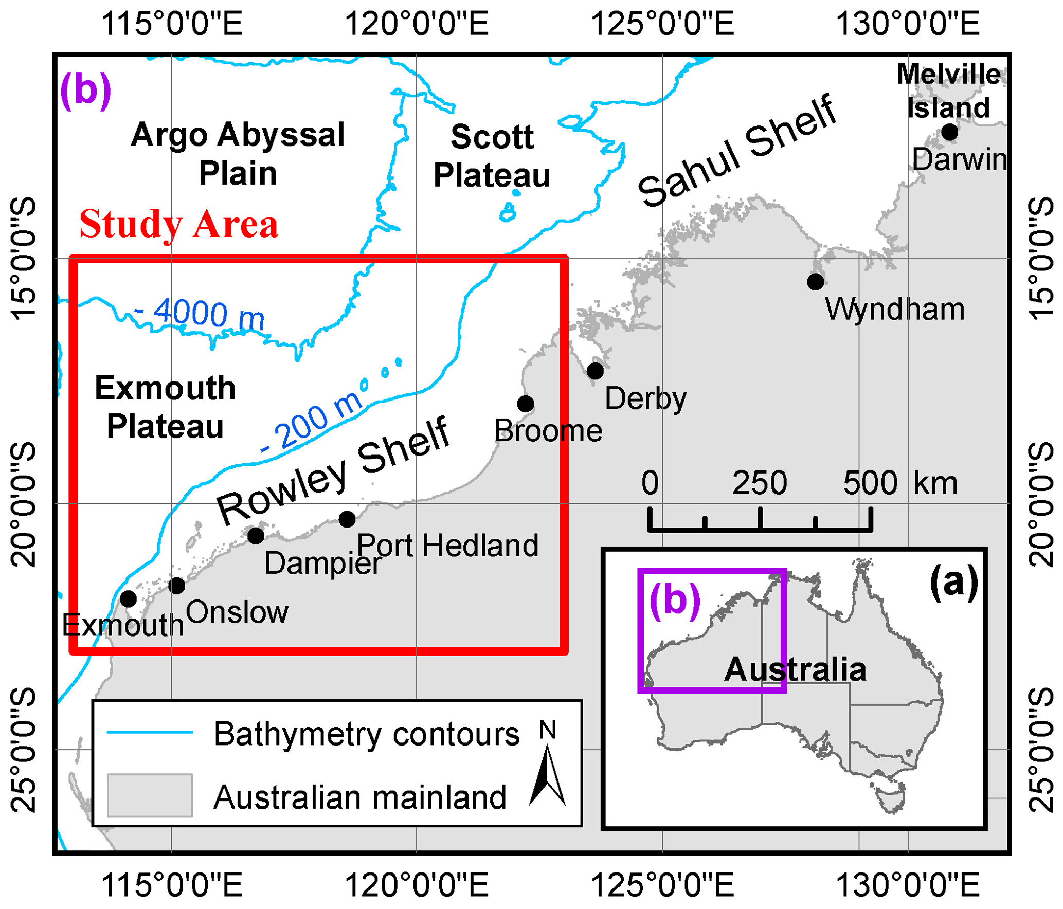
Figure 1 Location of the North West Shelf (NWS) of Australia. The area of interest covers the Rowley Shelf (southern half of the NWS) and the adjacent plateaus.

Investigations into the modern depositional environments of the NWS typically cover relatively small areas. Some regional studies exist, but they almost solely build on sparse seabed samples (Carrigy and Fairbridge, 1954; Jones and Australian Government Publishing Services, 1973; Dix, 1989; James et al., 2004; Baker et al., 2008). This observation can be explained by the limited coverage of open-source high-resolution geophysical datasets (Fig. 2), which in turn can be explained by the prohibitive cost of acquiring such datasets.

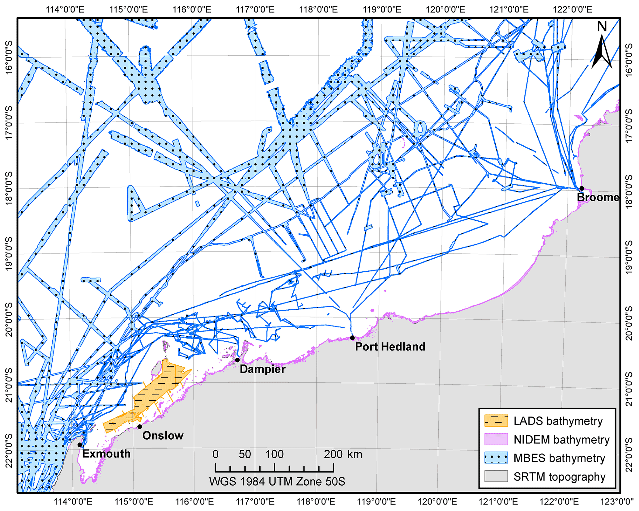
Figure 2 Public data available within the study area including Laser Airborne Depth Sounder (LADS) lidar bathymetry, the National Intertidal Digital Elevation Model (NIDEM; Bishop-Taylor et al., 2019), multibeam echosounder (MBES) bathymetry (Spinoccia, 2018), and Shuttle Radar Topography Mission (SRTM) data (Gallant et al., 2011). ENC navigation charts and the Australian Topography and Bathymetry Grid from Whiteway (2009) cover the entire area.

Geoscience Australia and the AusSeabed community are leading the effort to map the seabed around Australia via the acquisition and distribution of multibeam echosounder (MBES) bathymetry (Spinoccia, 2018). Currently, less than 25 % of Australian waters have been mapped using high-resolution techniques (Picard et al., 2018). Along the NWS, mapping coverage drops below 15 %. The integration of low-resolution and multi-source datasets can however allow the interpolation of high-resolution grids and therefore help improve the extent of mapped areas. Based on this approach, high-resolution bathymetry compilations were created over the Sahul Shelf, the Northern Territory, and the Great Barrier Reef using MBES data, airborne lidar bathymetry (ALB) surveys, satellite-derived bathymetry (SDB) data, and singlebeam echosounder surveys (Beaman, 2017, 2018).

The intent of this research was to follow a similar approach to create the first high-resolution bathymetry compilation across the Rowley Shelf and in doing so complete the existing work conducted over the Sahul Shelf by Beaman (2018) to provide full bathymetric coverage over the NWS. The main challenge to generating such a compilation is that the underlying high-resolution bathymetry surveys have a limited coverage and most of the areas consist of resampled or interpolated low-resolution datasets. To work around this limitation, we developed an innovative workflow to derive high-resolution bathymetry from satellite images and 3D seismic surveys at a regional scale. The workflow was successfully applied to the area of interest, and the resulting product was integrated with pre-existing open-source datasets to create a regional 30 × 30 m digital elevation model (DEM) and a 10 × 10 m bathymetry grid over areas of 935 000 km² and 45 000 km², respectively.

The scientific objective of this paper is to introduce the compilation produced over the Rowley Shelf and the associated workflows used to produce this outcome. The dataset includes the derived DEM as well as the underlying datasets in their original resolution. In the following sections, we present the data selection and the workflows used to produce the satellite-derived bathymetry and the seismic-derived bathymetry, as well as the processes adopted to compile a seamless high-resolution DEM. Quality check processes and discussions on the vertical and positional accuracy are presented for each dataset included in the compilation.

2 Processing tools

Source datasets presented in this paper were processed using the Python programming language. Python scripts were developed using three key libraries: (1) raster and shapefile calculations build on ArcGIS™ geo-processing tools, accessed via the ArcPy library; (2) the scikit-learn library, an open-source machine learning Python library, was used to perform statistical analysis of the data; and (3) the required computations were dynamically split between the logical cores of the workstation using the Python “multiprocessing” module. While the workflows were fully integrated into scripts, each of the processing steps presented in this paper can be completed manually via ArcGIS™ and presumably using any other GIS (geographic information system) software. Software used for specific processing steps is presented in the relevant sub-sections.

3 Pre-existing datasets

3.1 Australian Bathymetry and Topography Grid

The Australian Bathymetry and Topography Grid (AusBathyTopo Grid) was released through Geoscience Australia in 2009 by Whiteway (2009) and covers the totality of the Australian waters and mainland with a pixel size of 9 arcsec (1 arcsec ≈ 30 m near the Equator). This bathymetry grid was developed using all available depth soundings acquired or collated by Geoscience Australia with 1 arcmin ETOPO and 2 arcmin ETOPO bathymetry (Whiteway, 2009). Within the area of interest (Fig. 2), the topography is based on the Australian GEODATA 9 arcsec DEM (Whiteway, 2009). The pixel size does not always reflect the resolution of the data as extended areas, especially in deep-water domains, were interpolated from sparse data points.

3.2 SRTM-derived digital elevation model

Geoscience Australia produced the land surface topography using Shuttle Radar Topographic Mission (SRTM) data acquired by NASA in February 2000 (Farr et al., 2007; Gallant et al., 2011). The data were produced by Gallant et al. (2011) using an automated process to remove the vegetation from the original SRTM data and were released in 2011 as a 1 arcsec grid.

3.3 Multibeam echosounder bathymetry

MBES bathymetry acquired around Australia by numerous institutions has been collated and merged by Geoscience Australia (Spinoccia, 2018). This MBES dataset, which covers limited areas (Fig. 2), is regularly updated and is available as a 50 × 50 m grid. The distance between the recorded points of a beam increases with the depth and vice versa (Lurton, 2002); hence the average pixel size of 50 m used by Geoscience Australia does not always correspond to the actual resolution of the data (i.e. the points can be spaced by only a few centimetres in the shallowest waters). To overcome this issue, the native xyz data were obtained from Geoscience Australia and re-gridded using the root square of the average point density of each survey line as the pixel size. In some instances, where xyz files were not available, the re-gridded datasets were complemented with the 50 m grid.

3.4 National Intertidal Digital Elevation Model

The National Intertidal Digital Elevation Model (NIDEM) was compiled by Bishop-Taylor et al. (2019) using the Inter-Tidal Extent Model (ITEM) developed by Sagar et al. (2017, 2018) and integrates 30 years of Landsat images. The grid has a pixel size of 25 × 25 m and covers intertidal areas (Fig. 2) typically varying between +5 and −5 m mean sea level (MSL).

3.5 ENC navigation chart

Electronic nautical charts (ENCs) cover virtually the whole area of interest and were sourced from the Australian Hydrographic Office (AHO). Depth soundings extracted from the charts constitute a unique source of verified water depth (hereafter “depth”) measurements and can be used to calibrate other surveys. ENC depth point density varies significantly depending on the distance from the coast and proximity to highly navigable and/or populated coastal areas. On average, the distance between two measurements varies between 500 and 5000 m. Unlike other datasets that are reduced to MSL, navigation charts are referenced with respect to the lowest astronomical tide (LAT). To ensure the proper use of this dataset, all depth soundings were converted from LAT to MSL using the Australian Coastal Vertical Datum Transformation (AusCoastVDT) software, provided by the Intergovernmental Committee on Surveying and Mapping (ICSM). The software allows the conversion between vertical datums down to a depth of approximately 500 m (CRCSI and FrontierSI, 2019). Beyond that depth, the vertical uncertainty related to the datum is considered below the vertical accuracy of the depth sensors and hence of negligible impact.

3.6 Open-source LADS airborne lidar bathymetry

Laser Airborne Depth Sounder (LADS) data were collected from the Western Australian Government Department of Transport. The data were acquired by Fugro LADS Corporation in the vicinity of Onslow and Barrow Island. Surveys were conducted between 1998 and 2002 and cover an area of ∼ 4200 km². The spatial resolution of the data varies but is typically < 5 m.

4 Seismic-derived bathymetry

4.1 Overview

Australia's North West Shelf has been extensively surveyed using 3D seismic techniques, with the shelf between Exmouth and Broome now covered by ∼ 325 000 km² of 3D seismic survey (Paumard et al., 2019b). Under Australian legislation, most of this extensive dataset is publicly available through Geoscience Australia. The bathymetry data can be derived in two ways, either by extracting the first seismic reflection from the data themselves (which typically represents the seafloor) or by compiling the depth measurements from the vessel echosounder. The resulting datasets are referred to as reflection-derived bathymetry and navigation-derived bathymetry, respectively.

4.2 Reflection-derived bathymetry

4.2.1 Data source

Open-file seismic data were provided by Geoscience Australia. In total, 26 publicly available 3D seismic surveys were processed (Fig. 3). Additional surveys are integrated as they become available.

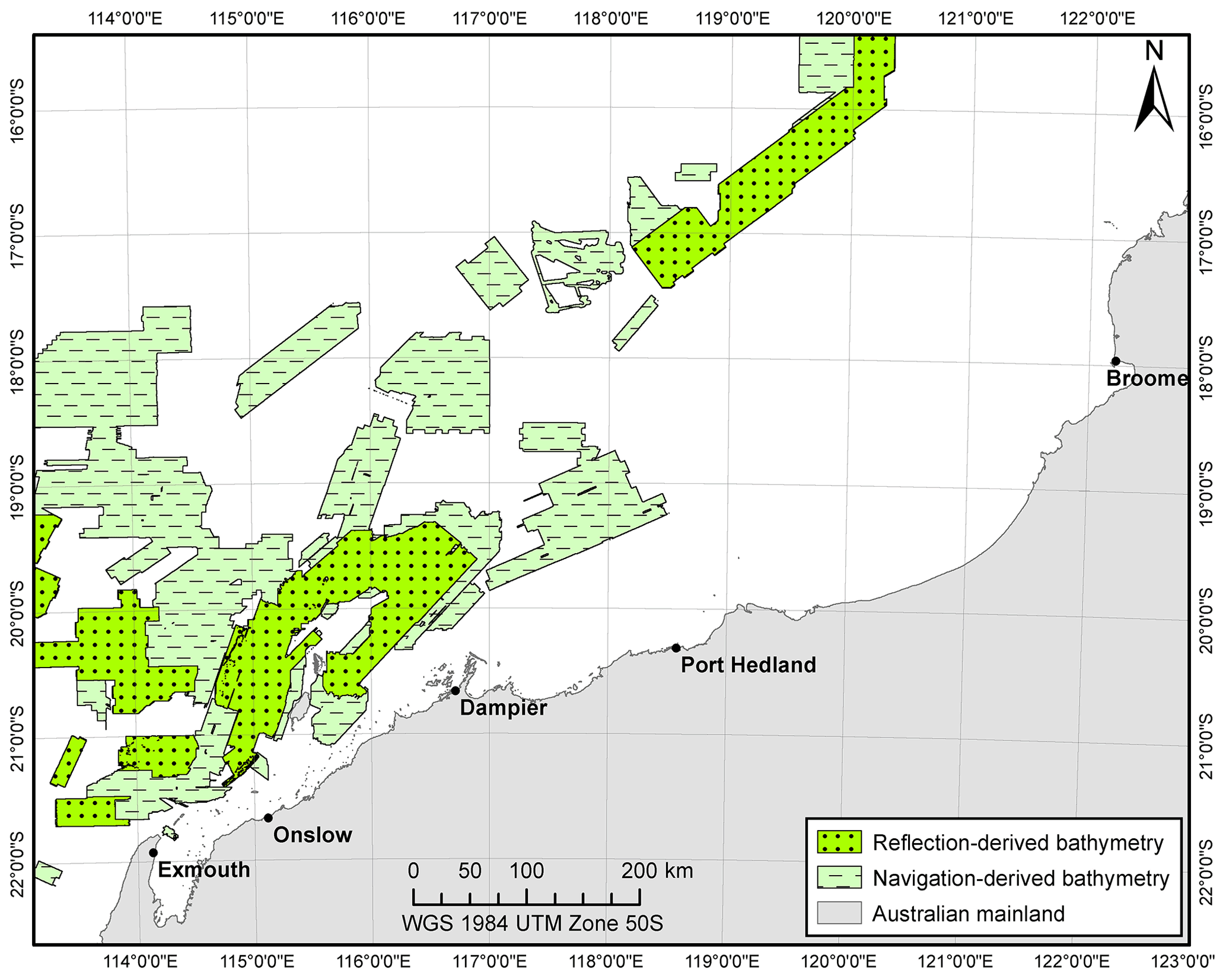
Figure 3 Extent of the reflection-derived and navigation-derived bathymetry. All areas covered by reflection datasets are also covered by navigation datasets. For data sources, see Sect. 4.2.1 and 4.3.1.

4.2.2 Data processing

The reflection-derived bathymetry extraction was performed using PaleoScan™, a full-volume seismic interpretation software. The interpretation is performed semi-automatically using similarities between adjacent seismic traces to generate an unlimited number of horizons within a chronostratigraphic framework (Paumard et al., 2019a). In this case, the workflow focused on the upper 500 ms (TWT, two-way time) of each seismic survey to optimize the resolution of the seafloor horizon.

Seismic horizons were subsequently converted from the time domain to depth domain. Due to the lack of regional water-column velocity profiles, an average velocity of 1500 m/s was obtained by averaging the nominal velocities specified in the navigation files of the surveys. The resulting velocity, while averaged from indirect sources, is comparable with values used in the literature to perform similar conversions (Mosher et al., 2006; Jibrin et al., 2013; Power and Clarke, 2019). The pixel size of the reflection-derived bathymetry grids corresponds to the spacing of the seismic traces and is generally comprised between 12.5 and 37.5 m.

4.2.3 Data limitation

The geometry of multichannel seismic survey acquisition systems appears to result in a reduction of the vertical accuracy in depth of less than 150 m. As depth reduces, the bathymetry becomes increasingly noisy and morphologies start to be vertically distorted, to the point where the relative height of seabed features can be multiplied by a factor of 5 compared to MBES data (Fig. 4b). Similar patterns were identified by the US Bureau of Ocean Energy Management in the seismic-derived bathymetry they generated over the Gulf of Mexico (Kramer and Shedd, 2017). In addition, sound velocity varies in the water column depending on the salinity, temperature, and pressure of the seawater (Leroy, 1969). Therefore, the use of a constant velocity to perform the time–depth conversion cannot capture local variations in the velocity profile and may result in a local underestimation or overestimation of the depths.

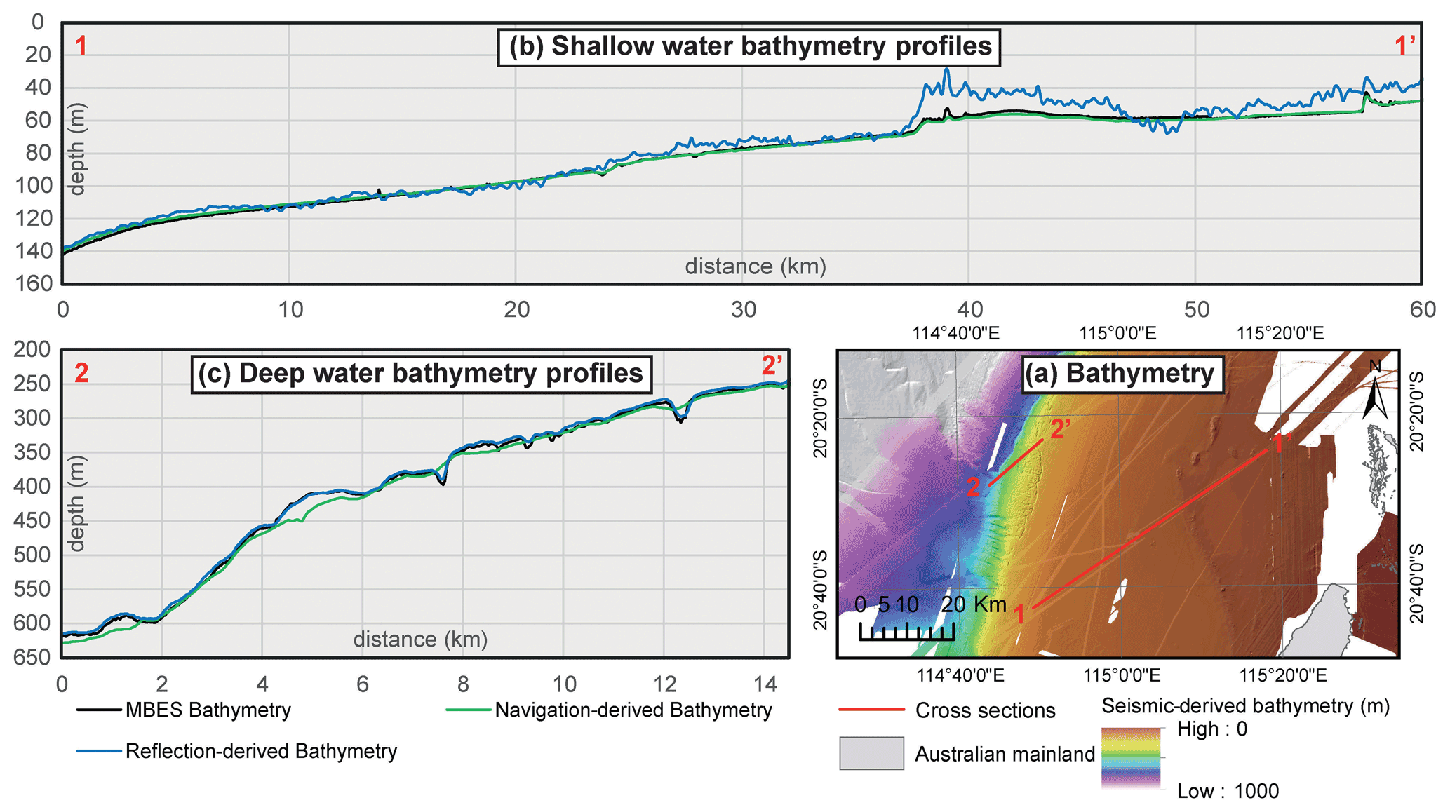
Figure 4 Comparison of the navigation-derived and reflection-derived bathymetry with MBES surveys in the vicinity of Barrow Island (a). Reflection data are heavily distorted in shallow waters (cross section b, from km 37), whereas navigation data are over-smoothed in deep waters (cross section c, km 0–9). For data sources, see Sects. 3.3, 4.2.1, and 4.3.1.

4.3 Navigation-derived bathymetry

4.3.1 Data source

P1/90 files are generated during the seismic acquisition and contain navigation-related information which include, for example, the coordinates of the vessel, source, receivers, and subsequent common mid-points. Each entry is associated with a depth measurement from the on-board echosounder (The Surveying and Positioning Committee, 1990). These files are, in most cases, publicly available, making them a powerful input for the generation of bathymetry at a regional scale.

Geoscience Australia (GA) has previously undertaken the compilation of the depth measurements from both 3D seismic and 2D seismic navigation files into a database. This product was made available to the project but did not include navigation data from the latest 3D seismic surveys. The navigation files from the missing surveys were subsequently sourced from the National Offshore Petroleum Information Management System (NOPIMS) data portal (http://www.ga.gov.au/nopims, last access: 21 March 2020). In total, 232 navigation files were collected from 3D seismic surveys within the area of interest (Fig. 3).

4.3.2 Data processing

During seismic acquisition, whenever a shot point is acquired, the coordinates of the different part of the acquisition system are recorded in the navigation files and are associated with the depth value recorded by the echosounder (The Surveying and Positioning Committee, 1990). Some parts of the acquisition system can be hundreds of metres from the actual echosounder location, leading to the creation of a significant mismatch between the actual location of the depth measurements and their coordinates (Fig. 5a). In several instances, this information was not properly recorded in the file (e.g. either the field is empty or the coordinates from the echosounder are not recorded or are at the wrong location). The P1/90 files were resultantly filtered in an iterative process to check if the depth values were properly recorded at the echosounder location and, if not, to use the values from the closest recorded point on the vessel. Doing so significantly reduced the spatial offset between the acquisition lines (Fig. 5b).

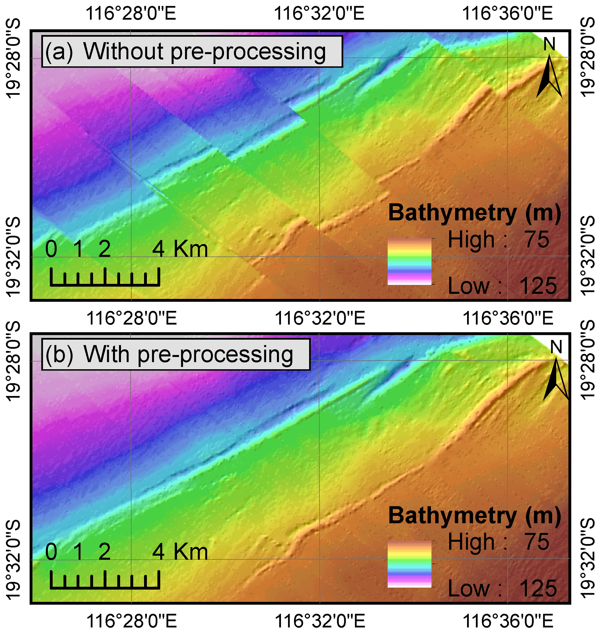
Figure 5 Comparison of the navigation-derived bathymetry generated using raw navigation files (a) or filtered (i.e. pre-processed) navigation files (b) from Demeter 3D survey. With raw navigation files, depth measurements are sometimes associated with the coordinates of the seismic receivers which can be located hundreds of metres behind the vessel, hence creating a “banded” pattern. During the filtering process, depth measurements were re-aligned with the vessel position. For data sources, see Sect. 4.2.1.

Depth measurements from the navigation files were then interpolated and gridded using the ArcGIS™ inverse distance weighted algorithm. Hengl (2006) suggests that the ideal pixel size to interpolate a scattered cloud of points is the average minimum distance between two points divided by 2. However, this formula often provided inaccurate results due to the geometry of the modern marine seismic surveys: data points are typically recorded every 6.25 to 25 m along acquisition lines that are spaced by multiple times this value (Vermeer, 2012). The minimum distance between two points is consequently not representative of the overall point density. The formula was modified to instead use the root square of the average area occupied by a point divided by 2. Navigation-derived bathymetry grids typically have a pixel size ranging between 30 and 50 m.

4.3.3 Data limitation

The geometry of modern marine seismic surveys was taken into account in the definition of the ideal pixel size, but the gap between adjacent acquisition lines was sometimes too important compared to the point spacing along these lines to result in an accurate bathymetry grid. In such instances, interpolation artefacts marking the acquisition lines can be seen on the grids. Overall, the navigation-derived bathymetry tends to become smoother as the depth increases (Fig. 4c).

It is also often unclear from the navigation files what level of correction was applied to the depth measurements. In some cases, it was stipulated whether the recordings were corrected for the roll, tides, and waves. However, in most cases, this information was not available, making it impossible to have a homogeneous correction process for all surveys. Finally, the headers of some of the files suggest that some measurements may have been converted from the time to depth domain using a constant value instead of site-specific velocity profiles, resulting in a possible overestimation or underestimation of the depths.

4.4 Data calibration

Given that seismic data are archived in time (ms), the reflection-derived bathymetry lacks a consistent vertical reference system, and a vertical offset of several metres can often be observed between the produced bathymetry grids. Likewise, even though navigation files are supposedly reduced to the MSL vertical datum, it is common to observe similar vertical offsets between surveys. The initial intent was to reduce all datasets to MSL using the depth soundings from the navigation charts as calibration points. However, in most cases, this method presented two limits: (1) the point density is often very low in deep waters, meaning that fewer than 10 points generally intersect a given 3D seismic survey, and (2) the validity of the ENC depth soundings is sometimes questionable as vertical offsets of tens to hundreds of metres were locally observed with MBES bathymetry grids. Depth soundings from ENC tiles were subsequently complemented with depth values from MBES bathymetry surveys. MBES surveys having a limited coverage; many seismic survey areas were intersected by neither ENC data points nor MBES surveys. The reflection-derived and navigation-derived bathymetry were therefore vertically shifted in an iterative process to obtain the best fit between the ENC depth soundings, the MBES bathymetry grids, and the surrounding seismic surveys.

4.5 Seismic-derived bathymetry compilation

Reflection-derived and navigation-derived bathymetry grids were merged in order to generate a consistent, seamless, seismic-derived bathymetry grid (Fig. 6a). In several areas, multiple surveys overlap. In such instances, due to the variability in resolution between surveys, only the values from the most reliable surveys were selected for inclusion in the final merged grid. Where appropriate, bathymetry grids were cropped to only include parts of them. The selection was performed considering two criteria. Firstly, the accuracy of the reflection-derived bathymetry varies depending on the depth. Thus, where depths are of less than 150 m, the navigation-derived bathymetry is preferred, whereas the reflection-derived bathymetry is preferred where the depths are deeper than 150 m. Secondly, surveys with the smallest line spacing and pixel size (i.e. high-resolution surveys) were prioritized. Prior to their inclusion, individual grids were resampled using a bilinear interpolation and a pixel size of 30 × 30 m.

Figure 6 The seismic-derived bathymetry (a) is mainly composed of navigation-derived bathymetry (b') in depth of less than 150 m and of reflection-derived bathymetry (c') in deeper waters. A total of 12 676 data points were extracted along a mesh from both MBES and seismic-derived bathymetry to assess the accuracy of the dataset using the coefficient of correlation (r²), the mean average error (MAE) and the root mean square error (RMSE) (d). The produced bathymetry marks a significant improvement compared to the Australian Bathymetry and Topography Grid from Whiteway (2009) (b vs. b' and c vs. c'). For data sources, see Sects. 3.1, 4.2.1, and 4.3.1.

4.6 Data accuracy

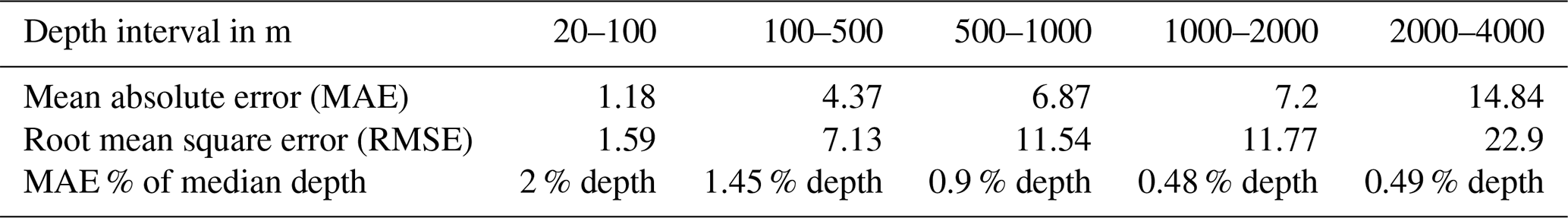
The 30 × 30 m bathymetry grid resulting from the compilation of the reflection-derived bathymetry and navigation-derived bathymetry was compared with the MBES bathymetry grids available on the NWS to assess its vertical accuracy (Fig. 6b, c, d). Values from both datasets were extracted along a 1000 × 1000 m mesh, representing a total of 12 676 points, and were plotted against each other. The result shows a very tight correlation between both datasets with a coefficient of correlation of 1.0, hence confirming the quality of the final product. The mean absolute error (MAE) gradually increases with the depth, but its relative percentage of the absolute depth decreases, meaning that the vertical accuracy of the data increases with depth (Table 1).

Table 1 Statistical metrics of the seismic-derived bathymetry.

5 Satellite-derived bathymetry

5.1 Overview

The utilization of satellite images to derive bathymetry has been the focus of numerous papers since the late 1970s and relies on the idea that since the light's wavelengths are not absorbed homogeneously by the water, it should be possible to derive the depths from the spectral content of the light reflected by the seabed. Out of the various methods developed, two main approaches have emerged: (1) the physics approach, which attempts to model the penetration of the light in the water and the resulting spectral content to estimate the bathymetry (Lee et al., 1994; Stephane et al., 1994; Brando et al., 2009), and (2) the empirical approach, which tries to correlate calibration points (i.e. true depth measurements) with the seabed reflectance (Lyzenga, 1978; Stumpf et al., 2003). Due to the extent of the area of interest and the high density of potential calibration points available (e.g. navigation chart depth soundings), the empirical method has been preferred over the physical approach for this study.

The IHO-IOC GEBCO Cook Book (International Hydrographic Organization and Intergovernmental Oceanographic Commission, 2019) presents a workflow to implement an empirical method using ArcGIS™ software. The method, which uses Landsat satellite images and calibration points from public navigation charts, builds on the log-ratio equation (Eq. 1) developed by Stumpf et al. (2003). The model is, according to the publication, less susceptible to the sea bottom effect than the Lyzenga model.

$$\begin{array}{}\text{(1)}& z=m_{\mathrm{1}}\left({\displaystyle \frac{\mathrm{Ln}\left(\text{Blue band}\right)}{\mathrm{Ln}\left(\text{Green band}\right)}}\right)-m_{\mathrm{0}},\end{array}$$

where m₁ and m₀ correspond to empirically determined gain and offset and Blue band and Green band to satellite image spectral bands.

The steps are as follows:

1. manual identification of the water–land separation and removal of the land using the infra-red (IR) spectral band,

2. generation of the band ratio using the green and blue spectral bands,

3. extraction of the band ratio values at calibration point locations,

4. calculation of the average band ratio value per true depth measurement,

5. visual definition of the depth of extinction (i.e. maximum depth of validity of the data),

6. generation of a linear regression line between the average band ratio values and true depth measurements,

7. application of the gain and offset of the regression line to the band ratio.

Following the guidelines from the IHO (International Hydrographic Organization and Intergovernmental Oceanographic Commission, 2019), the workflow of The IHO-IOC GEBCO Cook Book was used as a starting point in the development of the satellite-derived bathymetry. The main limitation of this workflow is that the gain and the offset are calculated at the scale of satellites image tiles (tens to hundreds of kilometres wide, depending on the satellite images used as input). These parameters therefore fail to capture spatial variation in seabed reflectance related to local environmental factors such as the type of substrate, the presence or absence of benthic communities, and the presence or absence of marine plants.

Furthermore, existing studies following a GEBCO-like workflow typically performed the processing steps manually and only applied the workflow to unique satellite images for unique locations (e.g. Pe'eri et al., 2014; Hamylton et al., 2015; Kabiri, 2017; Casal et al., 2018; Caballero and Stumpf, 2020). The result is strongly impacted by temporal events affecting either the sea surface or the water column and is therefore difficult to reproduce.

Other authors have attempted to circumvent such temporal artefacts by using multiple images acquired through a given period of time over a specific area. While heading in the right direction, these studies usually include a limited number of images (e.g. Chu et al., 2019; Evagorou et al., 2019; Poursanidis et al., 2019).

The number of manual steps required in the GEBCO workflow, as well the spatial and temporal uncertainties inherent to the empirical method, makes the processing of satellite-derived bathymetry over large areas challenging and of extremely variable accuracy.

In order to allow the production of reproducible seamless satellite-derived bathymetry at a regional scale, the workflow has been fully automated in Python scripts and was complemented by four processing steps, which aim to

1. improve and automate the water–land delineation using the normalized difference water index (NDWI) from McFeeters (1996) (Eq. 2),

2. improve and automate the calculation of the depth of extinction,

3. correct the data for spatial variation in the seabed reflectance using regional residual error models, and

4. remove the effect of temporal events by the generation of statistics model using multi-temporal images for each pixel.

$$\begin{array}{}\text{(2)}& \text{NDWI}={\displaystyle \frac{\text{Green band}-\text{NIR band}}{\text{Green band}+\text{NIR band}}},\end{array}$$

where Green band and NIR band correspond to specific spectral bands of satellite images.

5.2 Data selection

5.2.1 Satellite data

The Sentinel-2 constellation is composed of two satellites launched by the European Space Agency (ESA) through the Copernicus Programme in 2015 and 2017 to acquire high-resolution (10 × 10 to 60 × 60 m) multi-spectral images of the Earth surface (European Space Agency, 2020). The data acquired by the constellation, which have a position accuracy of 20 m on the ground, correspond to the highest-resolution product publicly available and were therefore selected for this study.

Sentinel-2 satellite images are available as tiles, each covering an area of approximately 100 × 100 km. In total, the area of interest is covered by 26 tiles. Images are composed of 13 spectral bands that are initially available as top-of-atmosphere reflectance products (Level-1c products). These images are not directly usable to derive the bathymetry as 90 % of the reflectance actually corresponds to the atmosphere (Gordon, 1983; International Ocean-Colour Coordinating Group, 2010). In December 2018 Copernicus started to release bottom-of-atmosphere products (Level-2a products) which are corrected for atmospheric effects using the Sens2Cor tool (Gatti and Galoppo, 2018). In April 2020, Sentinel Hub, a third-party company specialized in Earth observation, used the same tool to process from Level 1c to Level 2a all Sentinel-2 images acquired prior to December 2018 and decided to make them freely available (Milcinski, 2020). Thus, the complete catalogue of Sentinel-2 images is now fully and freely available as Level-2a products and can be used for further processing.

The penetration of the light in the water and hence the accuracy and the penetration of the produced bathymetry are highly dependent on seasonal environmental factors such as cloud cover, turbidity of the water, or roughness of the sea (Caballero and Stumpf, 2020; Zheng and DiGiacomo, 2017). It is therefore necessary to select an optimum time window to minimize the influence of such environmental factors on the depth model.

Climate data available from the Australian Bureau of Meteorology (Bureau of Meteorology, 2020) suggest that the optimum environmental conditions (i.e. low precipitation and wind speed) may occur between August and November each year. This timeframe was further reduced to the period ranging from August to October following a visual inspection of the data. A total of 1170 Level-2a modified Copernicus Sentinel-2 images acquired in August, September, and October 2017, 2018, and 2019, with a cloud cover of less than 1 %, were collected in April 2020 from Sentinel Hub, Sinergise Ltd, to be included in the bathymetry model. Out of the 13 available spectral bands, Sentinel-2 Band 02 (blue, central wavelength of 492.4 nm), Band 03 (green, central wavelength of 559.8 nm), and Band 08 (near infra-red, central wavelength of 832.8 nm) were used through the processing steps.

5.2.2 Calibration points

The determination of the parameters m₀ and m₁ from the Stumpf et al. (2003) equation requires true depth measurements to use as calibration points. The depth soundings extracted from the navigation charts represent the main source of widely spread depth measurements on the NWS. In total, more than 125 000 points are referenced within the area of interest. Locally, tidal areas are not fully covered by the navigation chart depth soundings. To overcome this, the dataset was complemented with data points extracted along a 500 × 500 m mesh from the NIDEM produced by Bishop-Taylor et al. (2019).

5.3 Data processing

5.3.1 Pre-processing

The pre-processing aims to attenuate the noise, masking the land and making sure that all meaningful information is used. It was performed in three steps, applied to the three bands (B02, B03, and B08) of all images used in subsequent steps. First, image types were converted from integer to float to make sure that cells can record decimal values. A low-pass filter, corresponding to a moving average of 3 × 3 pixels, was then applied to minimize the effect of speckle (pixel-based glint), following the recommendation from The IHO-IOC GEBCO Cook Book. Lastly, the NDWI was calculated using the equation from McFeeters (1996) (Eq. 2). Output values range from −1 to 1; positive values indicate the presence of open water, while negative values correspond to the land. The NDWI was used to clip out areas corresponding to the land by changing negative values to null.

5.3.2 Derivation of the initial bathymetry

A band ratio was then calculated using the first part of Stumpf et al. (2003) as presented in equation Eq. (3). The band ratio values must be tied with true depth measurements to determine the gain m₁ and the offset m₀ of equation Eq. (1). This is the key step of the data processing as it directly impacts the validity of the generated bathymetry.

$$\begin{array}{}\text{(3)}& \text{Band ratio}={\displaystyle \frac{\mathrm{Ln}\left(\text{Blue}\right)}{\mathrm{Ln}\left(\text{Green}\right)}},\end{array}$$

where Blue corresponds to Sentinel-2 Band 02 and Green to Sentinel-2 Band 03.

Figure 7 Illustration of the iterative process used to determine the depth of extinction of each satellite image and the resulting regression line. The gain and the offset of this line correspond to the parameters m₀ and m₁. For data sources, see Sect. 5.2.

Band ratio values were extracted at the calibration point locations and grouped by identified depth, rounded to the first decimal. For each unique depth, the band ratio values were filtered using the interquartile range score to remove outliers and averaged. The resulting averaged values were then plotted against the depth measurements from the calibration points. This revealed a linear correlation between the band ratio values and the calibration depths, up to a certain depth which is referred to as the depth of extinction. The depth of extinction (sensu International Hydrographic Organization and Intergovernmental Oceanographic Commission, 2019) corresponds to the depth beyond which changes in the satellite image reflectance can no longer reflect changes in depths and effectively indicates the maximum depth of validity of the method. The depth of extinction is different for each satellite image and varies depending on environmental factors such as the met-ocean conditions and the turbidity of the water. To allow batch processing of satellites images, the determination of the depth of extinction was automated via Python scripts and the use of a threshold coefficient of correlation (Fig. 7): a linear regression was calculated using all data points; if its coefficient of correlation was higher than 0.95, the regression was validated; otherwise it was recalculated using all depths minus 1 m. This maximum depth boundary corresponds to the theoretical depth of extinction being tested (Fig. 7). The process was repeated until the target coefficient of correlation was achieved or a minimum depth of extinction of 15 m was reached. In such an instance, the target coefficient of correlation was iteratively lowered by 0.05 and the process presented in Fig. 7 (i.e. the iterative lowering of the theoretical depth of extinction being tested) was repeated all over again and so forth until a target coefficient of correlation was validated. Ultimately each satellite image was associated with a depth of extinction and a coefficient of correlation.

The gain and the offset of the validated linear regression, which correspond to the parameters m₀ and m₁ of the Stumpf et al. (2003) equation, were applied to the band ratio to derive the bathymetry. These steps were performed for each satellite image.

5.3.3 Correction of the initial bathymetry

The generation of bathymetry grids is based on values of gain and offset averaged at the scale of satellite image tiles (100 × 100 km) that therefore do not capture semi-regional (kilometric to multi-kilometric) changes in the band ratio values (Fig. 8a) related to water-column turbidity, seafloor properties, atmospheric artefacts, etc. Such variations however follow trends; hence it is possible to correct some of their effects via the generation of an error model.

Figure 8 Illustration of the correction process applied to all Sentinel-2 images. The initial SDB grid (a) contains errors due to semi-regional spatial variation in the band ratio values that are unrelated to depth fluctuations. An error model between the original SDB grid and the calibration points was calculated to capture such errors (b). The model (b) was subsequently added to the original SDB grid (a) to generate the corrected SDB grid (c). For data sources, see Sect. 5.2.

Predicted depth values from the initial SDB data were extracted at the calibration point locations in order to calculate the absolute error between the predicted depths and the actual depths. A regional grid of the absolute error was then generated using the ArcGIS™ inverse distance weighted interpolation algorithm, where the weights are proportional to the inverse distance raised to the power p (Fig. 8b). The intent being to capture semi-regional trends and not local variations, low values of p (0.5) were used in the interpolation, meaning that the weight of distant points is maintained. Pixel sizes were calculated for each error grid using the root square of the average point density and are typically between 500 and 5000 m. The resulting grid, which highlights vertical offsets related to semi-regional errors, was then resampled to the satellite image resolution (10 × 10 m) using bi-cubic convolution and added to the generated bathymetry to obtain a corrected bathymetry grid (Fig. 8c).

Finally, values deeper than the extinction depth were removed from the grids. In order to take into account the vertical uncertainty in the data, the mean absolute error in the regression line was added to the depth of extinction, meaning that if an image had a depth of extinction of 29 m and a mean absolute error of 1 m, all values deeper than 30 m were removed.

5.3.4 Generation of the bathymetry stack

Processing steps to derive the corrected bathymetry data from the satellite images described in previous sections led to the generation of 1170 individual corrected bathymetry grids, each corresponding to the snapshot of a specific geographic area (tile) at a specific date (date and time of acquisition). Each grid is potentially affected by multiple temporal events and/or objects such as sediment plumes, waves, or ships which result in abnormal depth values (Fig. 9a, c, d, e). A statistical analysis was performed on the pixel values from the overlapping bathymetry grids to determine the most likely depth value of a given pixel, hence limiting the effect of such temporal events.

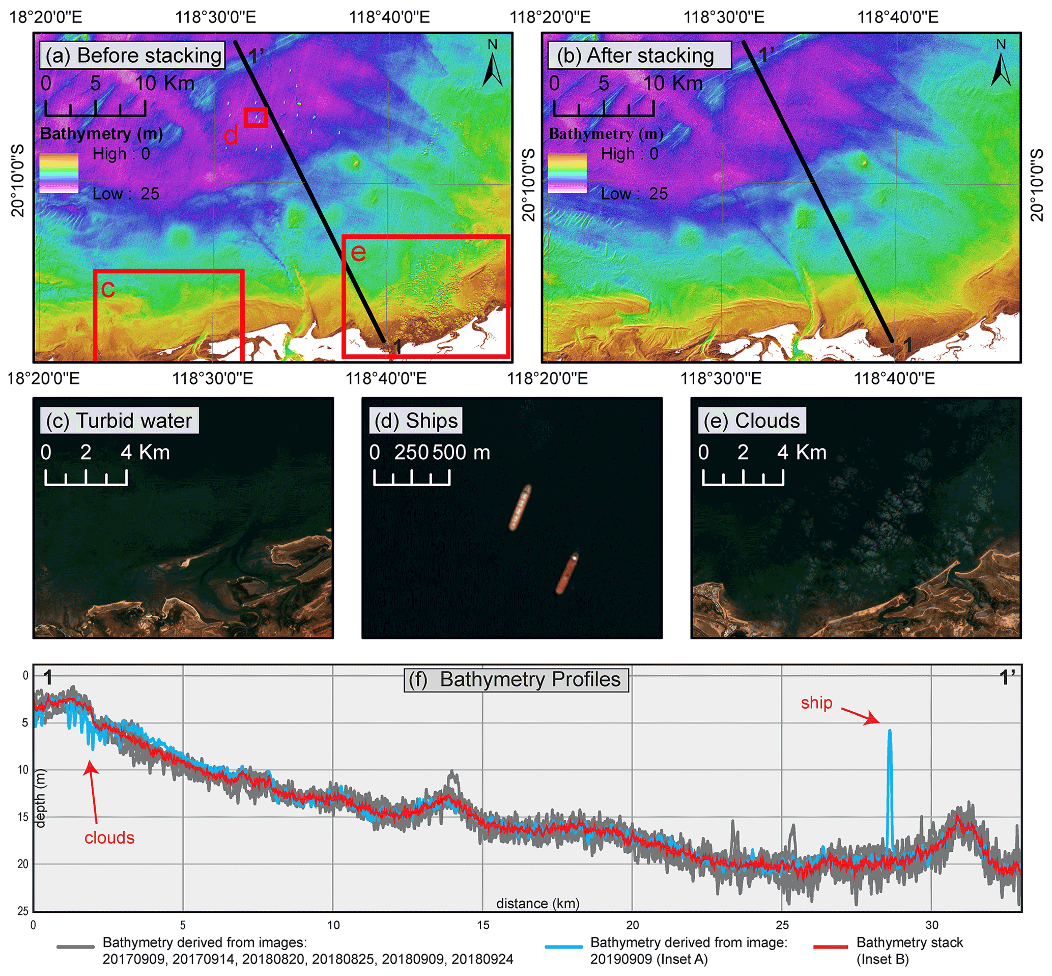
Figure 9 Illustration of the stacking process near Port Hedland (tile “KPC”). In the area, seven images met the specified coefficient-of-correlation threshold and were kept for the stacking. Each satellite image is affected by temporal effects that can be seen from red–blue–green (RGB) displays (see example c, d, e; Sentinel-2 L2a RGB image 20190909 was accessed through Sentinel Playground, the visualization portal of Sinergise Ltd) and on the resulting derived bathymetry (see panel a and cross section f, blue profile, derived from Sentinel-2 L2a image 20190909). The median value of all images was then calculated resulting in the removal of temporal artefacts (b, cross section f, red profile). For data sources, see Sect. 5.2.1.

For each tile, a minimum coefficient of correlation between the predicted depths and the calibration points was determined, and images with a coefficient below that threshold were discarded. Coefficients of correlation values used here to determine if an image should or should not be included in the stack were the values calculated during the derivation of the initial bathymetry, before the application of any types of correction, to avoid circular correlations. The threshold varied from one tile to another to reflect their respective specificities: tiles located in front of a delta, where the seabed is rapidly changing, have overall lower coefficient-of-correlation values than areas with no sediment supply. In that regard it was not possible to establish a firm rule, and the threshold was subsequently determined by the authors for each tile to obtain the best ratio between the number of images integrated in the stack and their respective coefficient of correlation. On average, the threshold was set at 85 %. Images with a coefficient below that threshold were discarded. In total, 222 images from 26 tiles met their respective selection criteria.

The median value of all selected grids was then calculated for each pixel. The compilation of these values corresponds to the final SDB grid after stacking (Fig. 9b and f).

5.3.5 Post-processing data cleaning

The water-land separation is based on the NDWI, meaning that any open water area was processed, including lakes and rivers. These water bodies, which are often not connected to the ocean, show very variable reflectance patterns and lack calibration points. This combination of factors often results in abnormal depth values. To minimize the occurrence of such artefacts, water bodies disconnected from the main ocean were removed from the final data (Fig. 10). Such filtering was performed as follows: (1) a raster domain shapefile (i.e. polygon coverage shapefile) was generated using the final SDB grid as input where each output polygon corresponds to an aggregate of pixels (i.e. a water body); (2) the largest polygon, which corresponds to the ocean, was extracted; and (3) it was used to crop the final bathymetry grid.

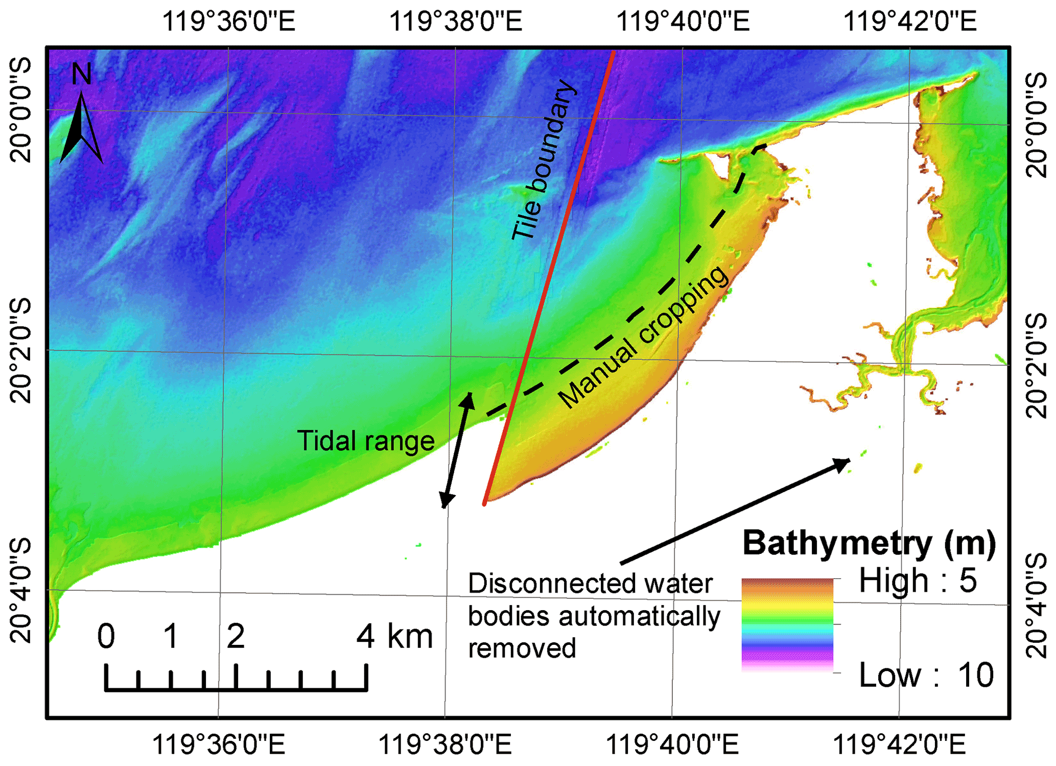
Figure 10 Illustration of the post-processing filtering. Given that each image is captured at a different tide, spatial mismatches can be observed near tile boundaries. Such artefacts only occur where images included in the stack do not capture the full tidal range. Upon review, they were removed manually. All disconnected water bodies were automatically removed. For data sources, see Sect. 5.2.1.

Given that band ratio values were calibrated using MSL reduced depth points, it was not necessary to correct the data for the tide vertical effect. However, since satellite images were acquired at different tides, sharp spatial contacts can appear along the coast at the interface between two images acquired at different tide ranges; the spatial area covered by the ocean is different on every image (Fig. 10). These contacts were manually smoothed (only a few were identified in the dataset).

5.4 Data accuracy

The final SDB grid was compared with ∼ 4200 km² of Fugro LADS data (acquired from the Western Australian Government Department of Transport) to independently evaluate its vertical accuracy (Fig. 11a). The comparison is based on a 500 × 500 m mesh that was used to extract depth values from both the LADS and the SDB grids. Depth values were then plotted against each other on a density chart. Overall, there is a good correlation between the SDB data and the LADS data with metrics indicating a coefficient of correlation of 91 % and a mean absolute error of 1.26 m (Fig. 11b).

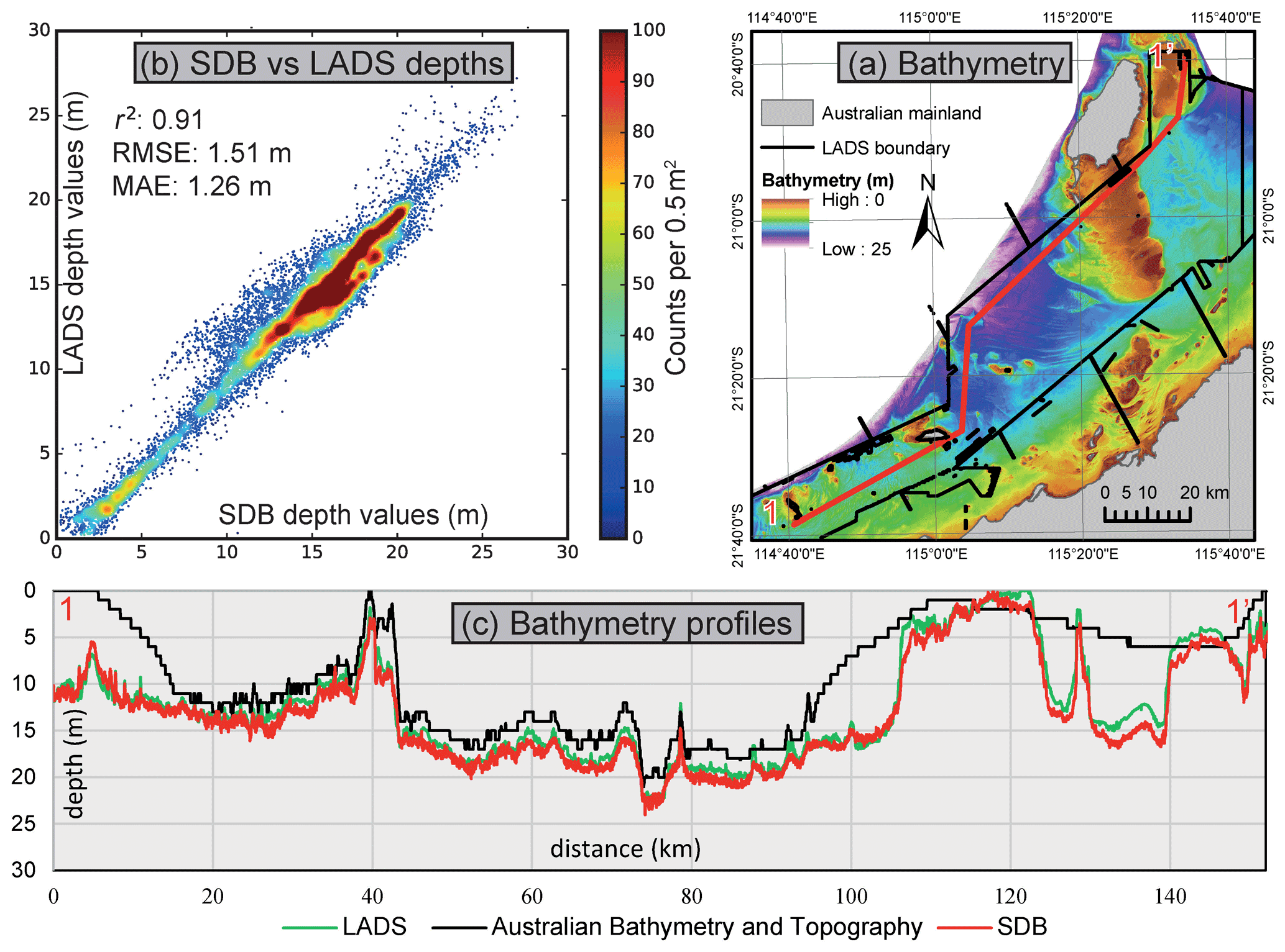
Figure 11 Assessment of the accuracy of the SDB using LADS data. In the vicinity of Barrow Island and Onslow, 4200 km² of LADS data overlaps the SDB data (a). Over 16 000 points were extracted along a mesh of 1000 × 1000 m from both datasets and plotted against each other to assess the accuracy of the SDB data (b). There is a strong correlation between both datasets as highlighted by the cross section (c). Some points seem to diverge from the main trend and reflect areas with a constant shift between the SDB data and LADS bathymetry (cross section (c), km 125 to 140). For data sources, see Sects. 3.1, 3.6, and 5.2.1.

It is nevertheless possible to observe that some points deviate from the general trend (Fig. 11c, cross section from 120 to 140 km). Upon review of the data, it appears that these points correspond to areas where there is a constant vertical shift between the calibration points and the LADS data and therefore between the SDB and LADS data. These areas were subsequently cropped out from the comparison area, resulting in an improved correlation between the SDB and LADS data, marked by a coefficient of correlation of 95 % and a mean absolute error of 1.01 m. This highlights the importance of the calibration points used in the process and indicates that the vertical accuracy of the SDB data is constrained by the vertical accuracy of the calibration points.

The LADS data coverage only represents a fraction of the 45 000 km² of processed satellite-derived bathymetry. To estimate the accuracy of the SDB data elsewhere, the standard deviation was calculated for each pixel using all bathymetry grids included in the final stack. The resulting mean standard deviation is 1.13 m, which is consistent with the accuracy calculated by comparing the SDB and the LADS data. The standard deviation appears to increase not only with depth (Fig. 12, Table 2) but also in areas with strong currents, water turbidity, a large tidal range, or potentially where major change in seabed type occurs (e.g. seagrass meadows), effectively highlighting areas that have changed significantly through the time interval included in the final stack. This suggests that the standard deviation layer could be used to better understand seabed conditions and could potentially, for example, help identify mobile bedforms.

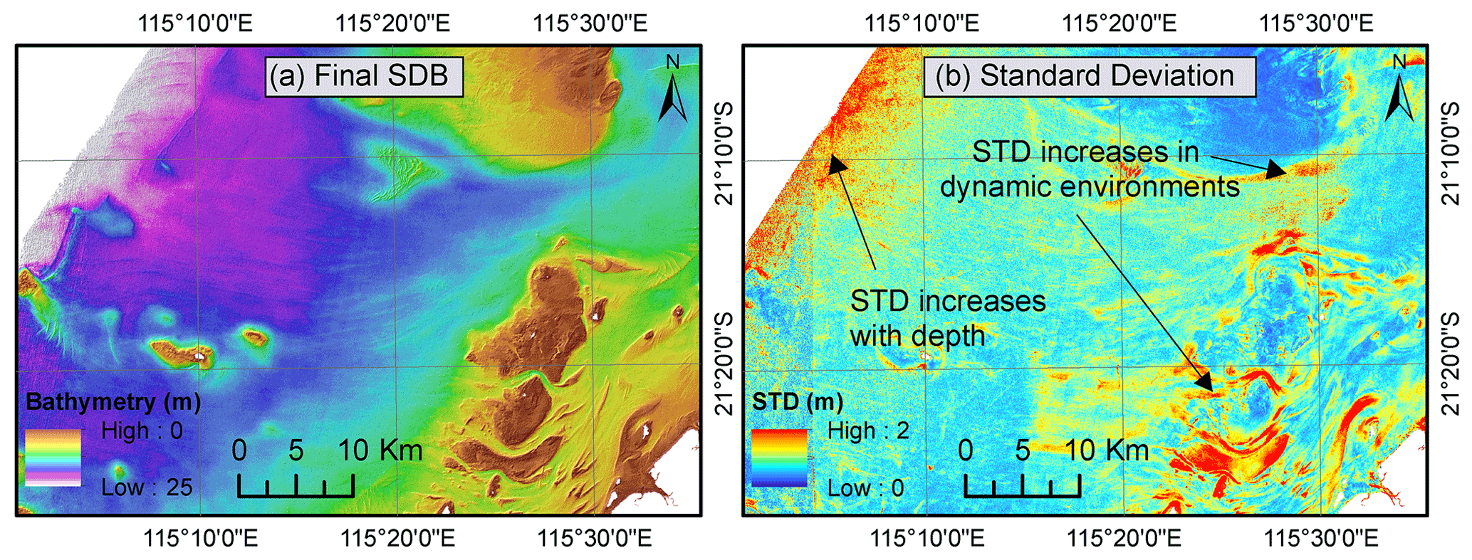
Figure 12 Illustration of the standard deviation grid (b) generated with the final SDB bathymetry (a). The grid illustrates the spatial variability in the final SDB grid accuracy. The standard deviation increases (and hence the accuracy of the bathymetry decreases) with depth as well as in dynamic environments where the seabed changed through the sensing period such as by tidal passes (b). For data sources, see Sect. 5.2.1.

Table 2 Mean standard deviation per depth range.

The worst-case scenario of an average vertical error of 1.26 m indicates that the vertical accuracy lies between 1 m + 2 % of the depth and 1 m + 5 % of the depth, depending on the depth range considered. This, combined with the positioning accuracy of the SDB of 20 m (positioning accuracy of the Sentinel-2 images (European Space Agency, 2020)), indicates that the dataset could potentially meet the criteria of Order 2 navigation surveys as defined by the International Hydrographic Office S-44 Standard (International Hydrographic Organization, 2020).

5.5 Data limitation

The relative depth changes are linked to the resolution and quality of the satellite images, but the absolute depth values are related to the calibration points, meaning that the absolute vertical accuracy of the SDB data is tied by the vertical accuracy of the calibration points. Furthermore, the generation of a meaningful error model requires a minimum number of calibration points depending on the regional depth changes: if the vertical offset between two adjacent calibration points is too high, the error model may generate more artefacts than it removes. This was observed, for example, west of Exmouth. The error model was consequently reviewed for each tile and removed when deemed inaccurate. Overall, the error model was kept for 25 out of the 26 satellite tiles included in the area of interest.

Finally, the stacking process aims to remove the noise and temporal artefacts by combining multiples images that were acquired on different dates. This process is overall very efficient, but if the seabed has changed drastically over the sensing period, the mobile bedforms will be perceived by the algorithm as artefacts and will be smoothed out. Such behaviour has been observed at the mouth of the De Grey River delta, east of Port Hedland, where distributary mouth bars seem relatively active. Nevertheless, even at this location, the advantages of the stacking process surpass its limitations as it filtered out most of the water turbidity. The stacking process allows generating a standard deviation grid which illustrates the accuracy of the data. Standard deviation values are however very sensitive to the number of images included in the bathymetry stack. As such an area where only a few images were included in the stack may be associated with low standard deviation values that do not necessarily indicate that the data are of high accuracy.

The computing power and the storage capacity available to the research project limited the number of satellite images that could be efficiently processed. In that regard, images were carefully selected using climate data and cloud coverage thresholds to ensure the best images were considered. Nevertheless, including the complete Sentinel-2 catalogue and using cloud masks, hence allowing the inclusion of partly cloudy images, would presumably enhance the robustness of the model. Similarly, the current workflow builds solely on one band ratio. Recent work from Caballero and Stumpf (2019) suggests that the inclusion of multiple band ratios could improve the results.

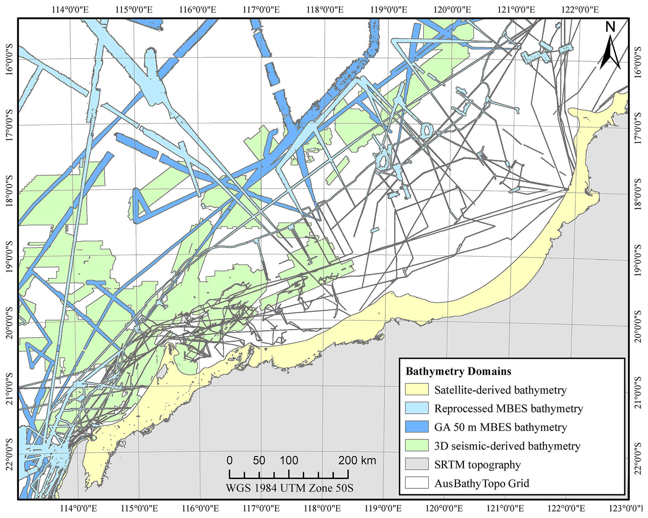
Figure 13 Lineage of the datasets included in the regional bathymetry compilation. For data sources, see Sects. 3, 4.2.1, 4.3.1, and 5.2.1.

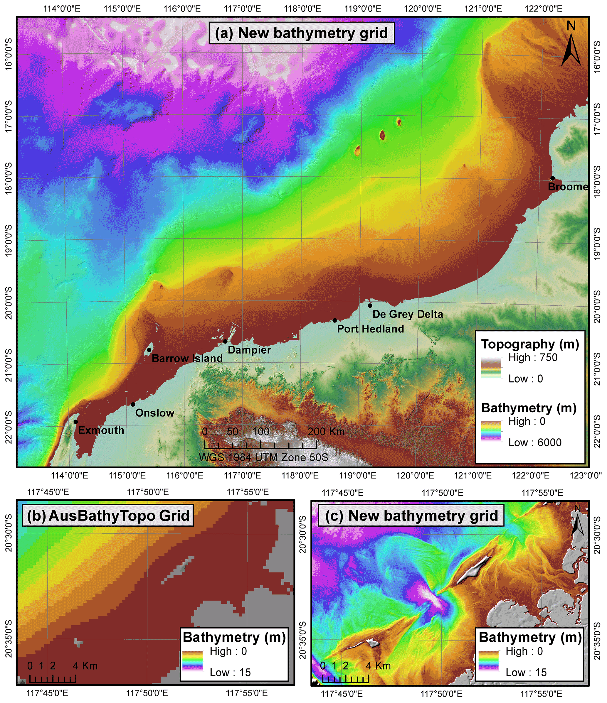
Figure 14 Overview of the produced DEM. Panel (a) displays the new bathymetry grid produced from the integration of the seismic-derived bathymetry, satellite-derived bathymetry, MBES bathymetry (from GA and reprocessed), and SRTM topography. Gaps are filled with the 9 arcsec Australian Bathymetry and Topography Grid. The compilation is a major upgrade of the pre-existing regional data (e.g. panel b vs. panel c). For data sources, see Sects. 3, 4.2.1, 4.3.1, and 5.2.1.

Table 3 Accuracy of the datasets included in the regional DEM.

6 Merging strategy

The creation of the regional DEM was based on the integration of the newly produced satellite-derived and seismic-derived bathymetry with the previously existing datasets. All datasets were reduced to MSL and resampled to a 30 × 30 m grid building on the UTM 50S WGS 84 horizontal datum and using bilinear interpolation. Selected datasets were included and ordered as specified in the following list (Figs. 13, 14a):

1. satellite-derived bathymetry

2. MBES bathymetry, reprocessed from xyz provided by GA

3. MBES bathymetry, downloaded from the AusSeabed website

4. seismic-derived bathymetry

5. the SRTM DEM

6. the Australian Bathymetry and Topography Grid.

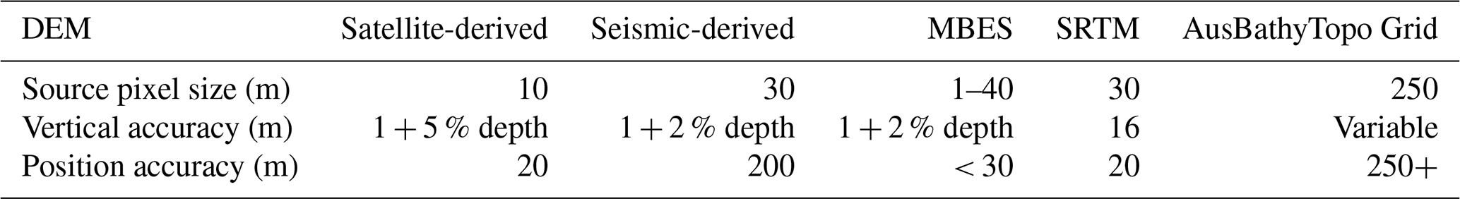
The NIDEM and Fugro LADS data and the depth soundings from ENC tiles were not included in the final merging as they were actively used in the calibration and validation process of the other datasets. The vertical and position accuracies of the dataset used to generate the regional DEM are specified in Table 3. Accuracy values were obtained using the source data metadata and specifications (International Hydrographic Organization, 2014; European Space Agency, 2020; Rodriguez et al., 2005; Whiteway, 2009) or were conservatively estimated using intersecting high-resolution datasets (i.e. LADS, MBES).

7 Data availability

All datasets can be downloaded at https://doi.org/10.26186/144600 (Lebrec et al., 2021). The repository includes the bathymetry compilation and the seismic-derived bathymetry with a resolution of 30 × 30 m as well as the satellite-derived bathymetry with a resolution of 10×10 m. The repository also contains grids presenting the standard deviation and the image count of the satellite-derived bathymetry. All grids are supported by lineage and metadata files. Other datasets presented in this paper can be accessed through their respective references and the Geoscience Australia AusSeabed data portal.

8 Summary

This research project led to the creation of a regional 30 × 30 m DEM over the Rowley Shelf and the adjacent plateaus. The dataset is based on the compilation of publicly available elevation measurements with seismic-derived and satellite-derived bathymetry produced using an innovative workflow and corresponds to a major upgrade of the pre-existing regional Australia Bathymetry and Topography Grid (Fig. 14b and c) published by Whiteway (2009). The vertical and positioning accuracy of the underlying datasets have been extensively assessed using high-resolution MBES datasets.

The produced datasets reveal submerged morphologies at a scale and resolution never achieved before on the NWS, allowing for a wide range of local and regional studies. Marine habitat mapping and oceanographic research rely heavily on high-resolution bathymetry data. So far, such studies have been limited to small areas, extrapolated afterwards to the rest of the shelf (Lyne et al., 2017; Brooke et al., 2017). Similarly, several attempts have been made to reconstruct the palaeo-geographic evolution of the shelf using low-resolution bathymetry (Larcombe et al., 2018; Ward et al., 2013; Whitley, 2017). In both cases, the inclusion of regional high-resolution bathymetry datasets will support the elaboration of regional-scale data integration and interpretation. In addition, recent studies have investigated the presence of submerged archaeological sites along the shelf (Benjamin et al., 2020; O'Leary et al., 2020; Dortch et al., 2019). The understanding of past coastal environments stemming from the study of this dataset could steer the identification of such sites of interest (e.g. O'Leary et al., 2020).

The DEM provides the full picture of modern sedimentary systems, from the source of the sediments (e.g. fluvial and carbonate systems) to their accumulation grounds along the shelf and in the basin. Parts of these modern systems can be used to better understand past sedimentary records (e.g. Paumard et al., 2020; Nyberg and Howell, 2016; Ainsworth et al., 2019), the geotechnical properties of marine sediments (e.g. Beemer et al., 2019, 2018; Senders et al., 2013), or geohazards affecting the area (e.g. Lane and Tyler, 2015; Hogan et al., 2017; Scarselli et al., 2019; Hengesh et al., 2013). Therefore, the integration of multi-source bathymetry data can constitute a step change and allow researchers to ponder their results with regard to the regional context and hence support the development of more reliable interpretations and models.

Workflows presented in this paper to generate the bathymetry compilation build on exclusively publicly available data, meaning that the method can be readily applied elsewhere in Australia and around the world. Additional datasets will be included in the compilation as they become publicly available.