the Creative Commons Attribution 4.0 License.
the Creative Commons Attribution 4.0 License.
 | 29 Oct 2021
High-resolution seasonal and decadal inventory of anthropogenic gas-phase and particle emissions for Argentina
S. Enrique Puliafito
Tomás R. Bolaño-Ortiz
Rafael P. Fernandez
Lucas L. Berná
Romina M. Pascual-Flores
Josefina Urquiza
Ana I. López-Noreña
María F. Tames
This work presents the integration of a gas-phase and particulate atmospheric emission inventory (AEI) for Argentina in high spatial resolution (; approx. 2.5 km×2.5 km) considering monthly variability from 1995 to 2020. The new inventory, called GEAA-AEIv3.0M, includes the following activities: energy production, fugitive emissions from oil and gas production, industrial fuel consumption and production, transport (road, maritime, and air), agriculture, livestock production, manufacturing, residential, commercial, and biomass and agricultural waste burning. The following species, grouped by atmospheric reactivity, are considered: (i) greenhouse gases (GHGs) – CO2, CH4, and N2O; (ii) ozone precursors – CO, NOx (NO+NO2), and non-methane volatile organic compounds (NMVOCs); (iii) acidifying gases – NH3 and SO2; and (iv) particulate matter (PM) – PM10, PM2.5, total suspended particles (TSPs), and black carbon (BC). The main objective of the GEAA-AEIv3.0M high-resolution emission inventory is to provide temporally resolved emission maps to support air quality and climate modeling oriented to evaluate pollutant mitigation strategies by local governments. This is of major concern, especially in countries where air quality monitoring networks are scarce, and the development of regional and seasonal emissions inventories would result in remarkable improvements in the time and space chemical prediction achieved by air quality models.
Despite distinguishing among different sectoral and activity databases as well as introducing a novel spatial distribution approach based on census radii, our high-resolution GEAA-AEIv3.0M shows equivalent national-wide total emissions compared to the Third National Communication of Argentina (TNCA), which compiles annual GHG emissions from 1990 through 2014 (agreement within ±7.5 %). However, the GEAA-AEIv3.0M includes acidifying gases and PM species not considered in TNCA. Temporal comparisons were also performed against two international databases: Community Emissions Data System (CEDS) and EDGAR HTAPv5.0 for several pollutants; for EDGAR it also includes a spatial comparison.
The agreement was acceptable within less than 30 % for most of the pollutants and activities, although a >90 % discrepancy was obtained for methane from fuel production and fugitive emissions and >120 % for biomass burning. Finally, the updated seasonal series clearly showed the pollution reduction due to the COVID-19 lockdown during the first quarter of year 2020 with respect to same months in previous years.
Through an open-access data repository, we present the GEAA-AEIv3.0M inventory as the largest and more detailed spatial resolution dataset for the Argentine Republic, which includes monthly gridded emissions for 12 species and 15 stors between 1995 and 2020. The datasets are available at https://doi.org/10.17632/d6xrhpmzdp.2 (Puliafito et al., 2021), under a CC-BY 4 license.
- Article
(12785 KB) - Full-text XML
-
Supplement
(4215 KB) - BibTeX
- EndNote


Many political, scientific, and professional efforts are devoted to understanding health and environmental problems. Air quality and global change are certainly two big concerns for the present (Al-Kindi et al., 2020; Haines et al., 2017). Sophisticated numerical models, chemical transport models (CTMs), and general circulation climate models (GCM) are used to identify and proof the underlying physics and chemistry of these environmental and social problems: by predicting the evolution and impact of atmospheric pollutants, as well as their geochemical cycles over space and time. From there on, these models are tools for evaluating and proposing mitigation and reduction strategies (Hallett, 2002; IPCC, 2014; Nakicenovic et al., 2000; Ravishankara et al., 2009; Solomon et al., 2009, 2020; Thompson et al., 2019).
Air quality models (AQMs) require the association of three types of basic information: meteorological data, static topography and land use data, and spatially gridded emission inventories. Meteorological boundary conditions are usually obtained from local measurements and/or global models such as ERA-Interim (European Reanalysis) and NCEP GFS (National Center for Environmental Prediction – Global Forecast System) reanalysis data. Surface terrain information can be obtained from satellite data such as those from the Shuttle Radar Topography Mission (SRTM3) (Rodriguez et al., 2005), whereas land use and surface cover data are available from the European Space Agency (ESA) map GLOBCOVER 2009 (Arino et al., 2010; Bontemps et al., 2011) and/or from regional reports (e.g., Voante et al., 2009). Emission data are generally obtained from national or international atmospheric emissions inventories (AEIs), which are arranged with different spatial and temporal resolutions, such as Emissions Database for Global Atmospheric Research (EDGAR) (Crippa et al., 2016; EDGAR, 2019), Evaluating the Climate and Air Quality Impacts of Short-Lived Pollutants (ECLIPSE) (Stohl et al., 2015), Community Emissions Data System (CEDS) (Hoesly et al., 2018), or the integrated assessment model Greenhouse gas–Air pollution Interactions and Synergies (GAINS) (Amann et al., 2011; Klimont et al., 2017). A comparison among GAINS, CEDS, and EDGAR is presented in McDuffie et al. (2020). A review for several national inventories in China is compiled in Li et al. (2017).
Global and regional AEIs require a permanent update in the spatial and temporal resolution of their data to keep track of the local socio-economic developments to improve the results of air quality models and/or global climate applications. Most inventories only present an annual account for a particular year; for example, Huneeus et al. (2020) compare time frame and available resolution of different emissions inventories for countries and cities in South America. National inventories usually include a compilation of greenhouse gases (GHGs) to comply with international agency requirements (i.e., UN-International Panel for Climate Change, IPCC). Nevertheless, as these technical reports focus on total nation-wide emissions for political and governmental protocols, these standard national inventories have low spatial resolution, normally reduced to a large subnational jurisdiction (i.e, provinces, or districts), and provide low to medium information on activity details. However, good practice in air quality determination and modeling requires the use of the finest possible spatial resolution grid, fine temporal resolution, and, whenever possible, technological details of the emissions sectors and activities as well. Gilliland et al. (2003) and De Meij et al. (2006) reported improved modeling results when using high spatial and temporal resolution. The finer the spatiotemporal resolution and the larger the number of species and sectors considered for the emissions, the better the air quality model performance achieved.
Local air quality models use an annual averaged static emissions inventory, whose initial constant primary sources are chemically transported with hourly dynamic meteorological data, resulting in pollution plumes that evolve following the weather conditions. Therefore, implementing a seasonally variable monthly regional emissions inventory will result in a remarkable improvement in the chemical prediction achieved by air quality models, such as the Weather Research and Forecasting (WRF) model coupled with Chemistry (WRF-Chem) (González et al., 2018; Grell et al., 2005; Ying et al., 2009), CALPUFF (Scire et al., 2000), WRF-CALPUFF (Lee et al., 2014; Tartakovsky et al., 2013), WRF-Chimere (Ferreyra et al., 2016), or AERMOD (Cimorelli et al., 2004; Kumar et al., 2006; Rood, 2014). This consideration is important, especially in cities and countries where air quality monitoring networks are scarce, as is the case for most South American nations, including Argentina.
Atmospheric emissions of short-lived climate pollutants (SLCPs), such as CH4, black carbon (BC), CO, non-methane volatile organic compounds (NMVOCs), NOx (NO2+NO), SO2, and NH3 affect air quality, ecosystems, and agricultural production and participate in global warming with important radiative effects. In addition, knowledge of the direct emissions of CO2 and N2O (and the abovementioned CH4) is important due to their dominant role as GHGs within future climate predictions. BC or soot comes from the incomplete combustion of biomass and fossil fuel being a significant constituent of fine particulate matter, an air pollutant associated with premature death and morbidity. BC has radiative effects by changing the surface albedo when it is deposited or by changing the optical properties of clouds (Myhre et al., 2009; Ramanathan et al., 2001). Methane is an important GHG with high radiative efficiency; it has natural and anthropic sources in particular as a component of natural gas, an increasing energy source (Shindell et al., 2004; West et al., 2006). CH4, CO, and NOx are precursors of tropospheric ozone, also one of the SLCPs, but since O3 is secondarily produced it is usually not included within primary gas inventories (Etminan et al., 2016; UNEP-WMO, 2011). Sulfate aerosols (formed from SO2 and NH3) and nitrate aerosols formed from NOx, NH3, and NMVOC emissions have cooling radiative effects (Isaksen et al., 2009). Therefore, reducing SLCPs (except CH4) would produce an improvement in air quality but would lead to postponing climate change mitigation, requiring some trade-off between air quality and climate change (Arneth et al., 2009). As is discussed in Stohl et al. (2015), SLCP emissions, in contrast to long-lived CO2, have different impacts on climate according to their geographic location and time of the year, changing their long-term climatic effect on both GHG and SLCP through multiple interactions (Jacob and Winner, 2009; Shindell, 2015). Thus, detailed spatial and temporal AEIs will help to improve the understanding of this regional and global interdependence.
At the local and regional scales, the detail of temporal and spatial knowledge of the activity included in an AEI will determine the quality of AQM result. For example, the particulate material emitted by a thermal power plant generating electricity will depend not only on the fuel (natural gas, gas oil, or coal) but also on the given generation technology (combined cycle, turbo steam, etc.). Similarly, the increasing use of nitrogen fertilizers in agriculture in Argentina in the last 20 years has allowed the expansion of the agricultural frontier, increasing yields and cereal production, but at the same time increasing the emissions of nitrous oxide and ammonia, leading to higher SLCP emissions. As a consequence, more accurate AEIs will contribute to evaluating the most efficient measures to reduce pollutants and to assess the economic and health impact of each activity.
This article presents a gridded emissions inventory for a dozen SLCPs and GHG species in Argentina with high spatial resolution (; approx. 2.5 km×2.5 km) and, for the first time, a monthly temporal resolution from 1995 to 2020, including many sectorial activity details compiled in several appendices. It is also a revised extended update and compendium of previously published emission inventories by Puliafito et al., (2015, 2017, 2020a, b) for the years 2014 and 2016, but incorporating additional detailed activities of the manufacturing sector and the monthly temporal evolution for most of the activities and sectors considered (Table A1). We will refer to this inventory as “GEAA-AEIv3.0M”: GEAA Argentine High-Resolution Inventory version 3.0 with monthly resolution”.
We compare our results with the Argentine GHG inventory for the Third National Communication of Argentina to the IPCC (TCNA, 2015), which includes annual GHG emissions from 1990 through 2014, which was updated in 2019 (TCNA, 2019), spanning from 1990 to 2016. Annual total emissions of GHG and air quality pollutants are also compared to the estimations presented in the EDGAR HTAPv5.0 inventory (Crippa et al., 2016, 2020; EDGAR, 2019) and the Community Emissions Data System (CEDS) (Hoesly, et al., 2018; McDuffie et al., et al., 2020).
This section describes the process of preparing the GEAA-AEIv3.0M inventory: how the data from the different activities were collected, their sources and references, the methodological procedure used to estimate the emissions to the atmosphere, and how the geographical allocation of each activity was performed. Details of each sector are presented in the Appendices and Supplement, providing only representative tables and figures in the main text. Table 1a shows all sectors and activities included in the GEAA-AEIv3.0M inventory, its corresponding IPCC2006 code, the subsections where it is described, and its geographical and temporal extension. Table 1b indicates all species included for each activity with their spatial and temporal resolution. Table 2 summarizes the names of national agencies and institutions whose activity data were considered here, as well as a compendium of the main acronyms used throughout the text.
Table 1(a) Sectors, activities, classification codes, and resolution considered in the GEAA-AEIv3.0M inventory. (b) Sectors, activities, and pollutants considered in the GEAA-AEIv3.0M inventory.
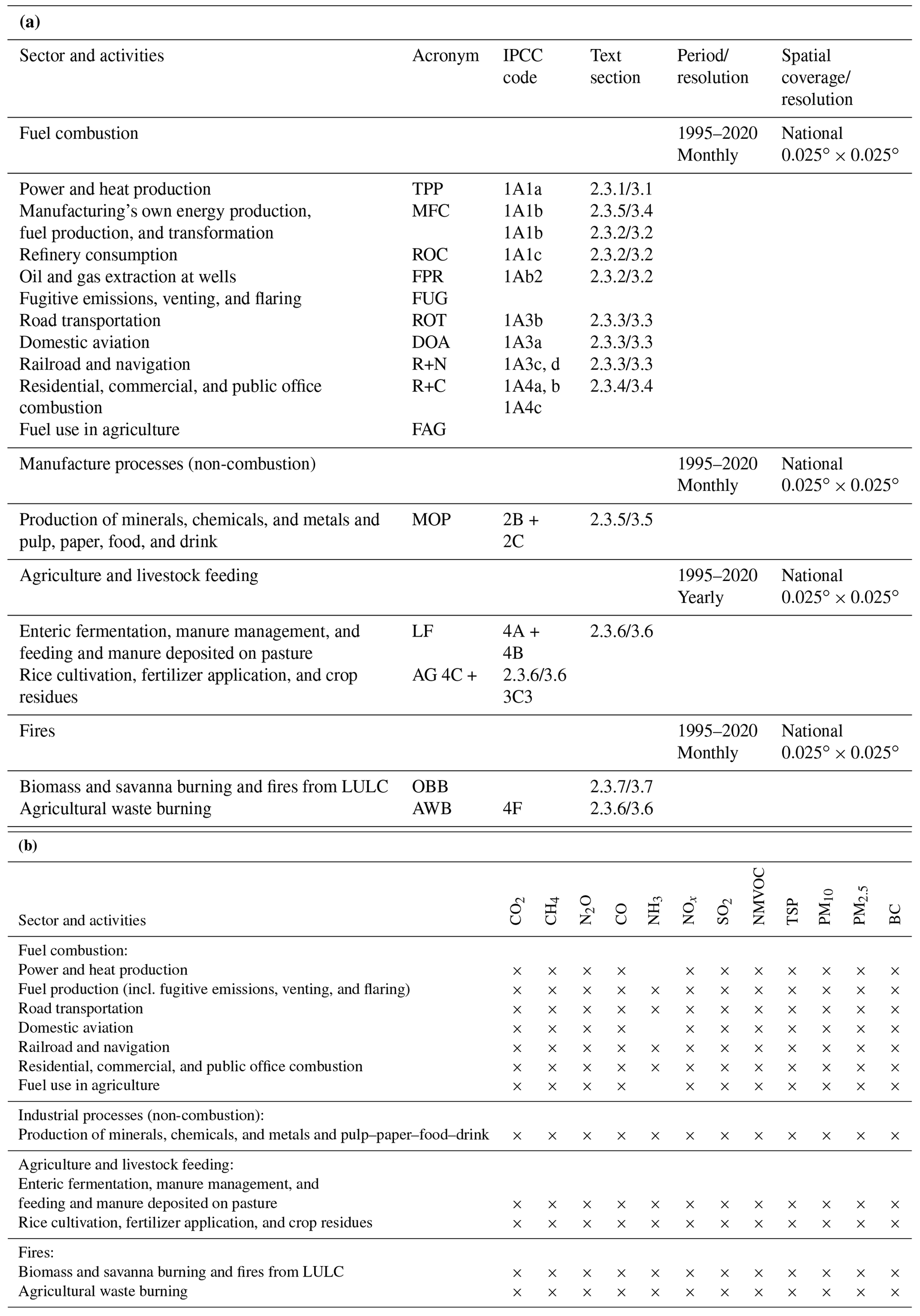
Table 2Abbreviations used in this text.

* Additional abbreviations are compiled in Table A2.
2.1 Study area and reshaping of databases
The inventory is focused on the activities performed on the continental territory and close coastal maritime area of the Argentine Republic (Fig. 1a). Argentina is located in the extreme south of South America covering 2 778 000 km2 (IGN, 2020). Its political organization includes 24 provinces and 524 departments or districts, split between rural and urban areas. Population information such as localities and census fractions is available in high resolution. All pieces of data were organized as a gridded map whose cells have a resolution of between 53 and 73∘ west longitude and between 21 and 55∘ south latitude. An EPGS4326, WGS84 mapping is used (Fig. 1a). Thus, the study area is made up of a regular grid of 1441×912 cells corresponding to the continental and coastal maritime sector of Argentina. Figure 1 also shows the different scales associated with the mapping process of the available information.
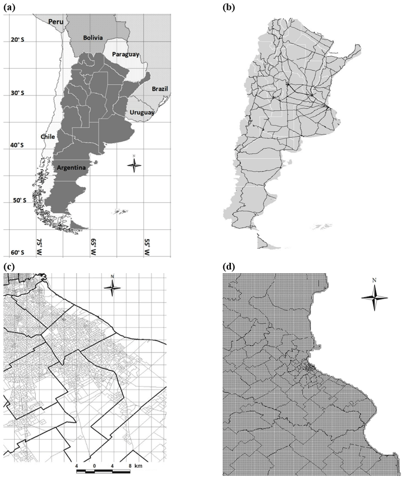
Figure 1Spatial coverage and scales used in this inventory: (a) geographical location of Argentina in South America (provinces in white outline), (b) main roads, (c) districts (black outline) and census fractions (grey outline), and (d) spatial grid with districts in background.
Depending on the spatial extent, power plants, industrial sources, or refueling gas stations can easily be associated with a geographical point and residential consumption and agricultural production with an area source, whereas transport emissions (roads and railways) are associated with a line with a length that can be on the order of hundreds of meters to thousands of kilometers. For air quality modeling purposes, these different source types were reshaped into a single database in the form of grid map. The resolution of the base information determines the size of the grid cell (in this case approx. 2.5 km×2.5 km). Area or line sources can either be included or not in a single cell. When sources sizes were greater than one cell (i.e., consumption or production is known at the district level), proxy known data were selected to spatially disaggregate that variable (i.e., land use, population). If the variable was smaller than one cell (e.g., small census radii data in urban areas), all the sources contained in that cell were added together (Figs. 1 and 2).
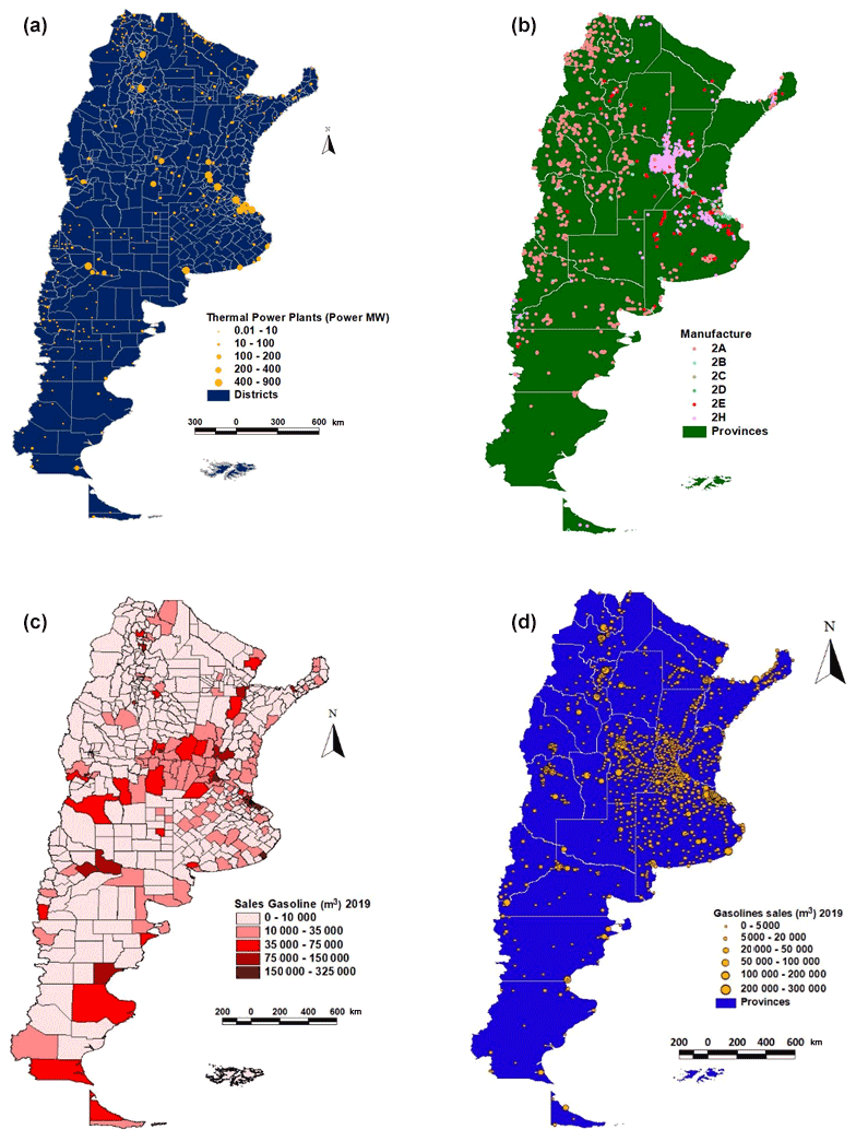
Figure 2Location of point sources. (a) Thermal power plants (districts in white outline). (b) Manufacturing industries (provinces in white outline). Manuf. code. 2A: cement, calcium, glass, mining; 2B: chemical; 2C: steel, iron, aluminum; 2D: car-painting; 2E: other non-specified, 2H: paper, food, beverages (see Table A3). (c) District distribution of annual gasoline sales for 2019. (d) Location of refueling gas stations and their individual yearly gasoline sales.
The activity data for each sector were obtained consulting official national organizations and reports (Table 2). These included the Statistics and Census Bureau (INDEC), the Ministry of Energy (MINEN), the Ministry of Agriculture and Livestock (MAyGN), the Animal Health Control Agency (SENASA), and the Ministry of the Environment (MINENV) through the Third National Communication of Argentina (TCNA, 2015) to the UNFCC, with the subsequent Biennial Updates (for 2014 and 2016).
Fuel production, processing, sales, and consumption for various sectors are available monthly from 1994 to present from public databases at MINEN. Electricity generation and fuel consumption at power plants are available monthly from 1994 to present at the energy distribution agency (CAMMESA) and the Energy Regulation Agency (ENRE). Industrial production is available mostly monthly since 1990 from the respective industrial chambers (see subsections). Transport data are available from several national transport regulation agencies (CNRT: public transport, navigation, and railroad; ANAC: domestic and international aviation).
2.2 Calculation approach
Depending on the specified detail, emission maps are constructed, in a bottom-up process, gathering activity data (i.e., fuel consumption, number of vehicles, energy generation), or top-down approach using national aggregated activities (i.e., population, total energy consumption, gross domestic product) and then applying specific emission factors (EMEP, 2019).
The activity data are organized by sectors with monthly resolution from January 1995 up to December 2019, and for some sectors they include several months in 2020, according to the available information. The general methodology applied is based on European regulations that are compiled in the European Monitoring and Evaluation Program (EMEP) (EMEP, 2013, 2019) and has been described elsewhere (Puliafito et al., 2015, 2017, 2020a). Briefly, emissions are calculated following the general Eq. (1).
where E is the total emission (i.e., Mg yr−1) for a pollutant p; A is the activity of sector i, for technology j; and is the emission factor for that sector, technology, and pollutant. For example, the emissions (Mg yr−1) of CO (p), corresponding to the annual consumption of gasoline (j), of the private automotive sector (i).
The inventory was calculated by each individual sector based on the following steps: first, identifying the source of the emission in its geographical coordinates (latitude and longitude); second, assigning the specific activity that contributes to this emission to each coordinate; third, developing a consistent monthly activity evolution; fourth, applying specific emissions factors for each species, source, and activity; fifth, organizing the information into a three-dimensional map (latitude, longitude, time); and sixth, developing indices, tables, figures, and statistics.
As mentioned above, air quality models (i.e., WRF-Chem) require fine spatial and temporal resolution (i.e., hourly information); however, the available original activity data are organized monthly in most cases. To obtain weekly and hourly profiles, whenever possible, we evaluated the temporality of each sectorial activity independently. For example, hourly and daily electricity consumption is available from energy distribution agencies. The evolution of road transport in large cities is also well known. This information allows us to produce an averaged interpolated hourly emission profile, which can later be used as a proxy for other sectors (i.e., use of natural gas for heating and cooking). Conversely, other sectors such as agriculture and livestock breeding are only available on an annual basis, and only lineal interpolation may be done to obtain monthly values. Similarly, sectorial information is spatially organized into districts. So, special care must be taken to discriminate the information into the merged gridded map. In the next methodological subsections, details are given for the spatial and temporal re-assignation.
2.3 Anthropic emission by activity sector
The calculation methodology for each subsector and activity is briefly described below. The data supporting the activity for each subsector, (i.e., monthly fuel consumption, household, technology, number of livestock), and other relevant information, were compiled and made available in an external repository as described in the Data availability section.
2.3.1 Electricity production sector
The activity and consumption of the electric thermal power plants (TPPs) are registered monthly in the Ministry of Energy (Minem, 2020) and in the electric distribution agency (Cammesa, 2020). The location of each power plant is well known; thus in a GIS format, these sources are represented as point sources (Fig. 2a). Power plant information included the available machines and technologies (CC: combined cycle; TV: turbo steam; TG: turbo gas; DI: diesel engine) and the respective fuel consumption for each machine (NG: natural gas; FO: fuel–oil; GO: gas oil; CM: mineral coal; BD: biodiesel) (Fig. 3a). The emission of each machine and plant is calculated according to Eq. (1), using the proper emission factors.
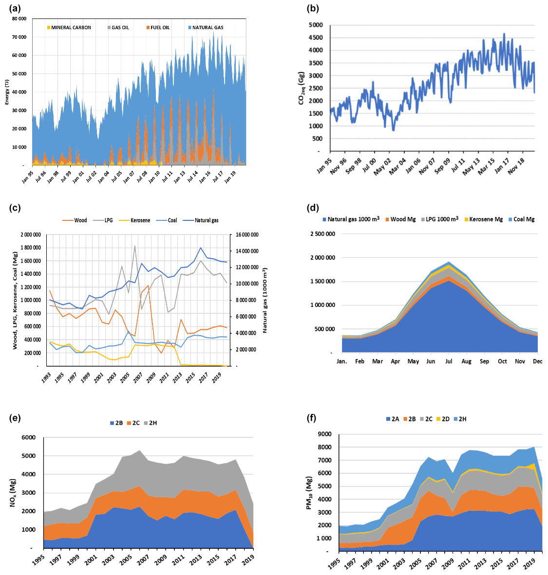
Figure 3(a) Evolution of monthly energy consumption by thermal power plants. (b) GHG emissions evolution (in terms of CO2eq Gg) from energy consumption at thermal power plants. (c) Monthly fuel consumption for residential and commercial sectors. (d) Seasonal average fuel consumption for residential and commercial sectors for the period 1995–2019. (e) Annual NOx emissions (in metric tons) from manufacturing activities. (f) Annual PM10 emissions (in metric tons) for manufacturing activities. Ref. manuf. codes: 2A: cement, calcium, glass, mining; 2B: chemical; 2C: steel, iron, aluminum; 2D: car-painting; 2H: paper, food, beverages (see Table A3).
2.3.2 Fuel production sector
Emissions from the production and transformation of fuels were calculated from consumption, venting, and flaring in refineries and the production from oil and gas in wells. Within the solid fuel production sector (1B1), we estimated the gross production of coal using the Argentine national energy balance (NEB). We applied two emission factors for mining and post-mining operation (18 and 2.5 m3 CH4 t−1 gross production of coal, respectively, according to IPCC Chap. 4), which are based on mining activity in Río Turbio, Santa Cruz (51.57∘ S, 72.31∘ E). The Ministry of Energy (Minem, 2020) maintains a monthly record of upstream production and extraction of gas and oil in the wells and downstream fuel production, refineries' consumption, and sales in the refineries. Emissions were calculated from refineries' consumption (in wells and refineries) according to the type of fuel consumed, using Eq. (1). Note that each well or refinery is represented as a point source, so the emissions are in their respective coordinate within our GIS format.
2.3.3 Transport sector
Emissions can be calculated by applying general emission factors by type of fuel and type of commercialization (Eq. 1) (EMEP, 2019) for a top-down national total account. However, an inventory dedicated to AQM requires the spatial (and temporal) allocation of consumption activity and emissions. We used a bottom-up approach using GIS software: where roads and railroads are represented by segments, airports, and navigation ports by points. Activity and emissions are first allocated in the respective segments and then integrated in the respective grids, as described below.
Road transport fuel consumption for each district (Fig. 2c) is available monthly for each type of fuel (gasoline, gas oil, natural gas, kerosene, and liquefied petroleum gas) and by type of commercialization (sale to the public, public transport, cargo transportation, and agricultural machinery) (data available in the MINEM database, Table 2). Additionally, monthly fuel sales are also available for each refueling gas station (RGS). Thus, we use the location and fuel sales of each commercial RGS (Fig. 2d) to estimate the spatial and temporal road transport activity. Road transport fuel consumption is directly proportional to vehicle kilometers traveled (VKTs) on each route. The routes are represented as segments on a GIS-type map (Fig. A1). These segments intersect the reference grid map (with resolution cells of ). Thus, in each cell there will be small segments that represent the route sections with their respective lengths and hierarchies. The spatial distribution of fuel consumption was carried out following Puliafito et al. (2015), who synthetically distributed the consumption of each RGS (FuelRGS) using a Gaussian function of variable width (Eq. 2), according to the type of fuel and location of the RGS (rural or urban). Then, apply a convolution (Eq. 3) to calculate the contribution of each RGS in each cell of the gridded map.
The estimated fuel consumption of each cell (FuelCONV) is distributed proportionally to the hierarchy of the routes (highways, main routes, residential and rural roads, etc.). Once the fuel consumption per cell has been obtained, the allocation of the VKTs will depend on the fuel efficiency by vehicle type and fuel R(c,k) and the length of each segment in the cell (Eqs. 4 and 5).
Fuel efficiency is calculated at the national and provincial levels, according to the balance of fuel consumption and quantity and type of vehicles. Since hierarchy and length are known for each segment, it is possible to calculate from Eq. (5) the number of vehicles per segment. Finally, the emission can be calculated using VKTs and proper emission factors (Eq. 6).
where is the emission factor for fuel burning (g m−3 of fuel consumed), and is the emission factor of each type of vehicle per kilometer traveled (g km−1) according to EMEP (2019). Figure 2c shows the fuel sales at the district level, and Fig. 2d shows the distribution of the fuel sales for each refueling gas station (RGS). Figure A1 shows the calculated VKTs for gasoline vehicles and the CO emissions, which are proportional to the VKTs. This procedure (Eqs. 2 to 5) is then iterated comparing the estimated vehicle flows with those counted by road maintenance agencies. Changes in the hierarchy weights (h in Eq. 5) or Gaussian function width (d in Eq. 2) were used to produce the convergence (Puliafito et al., 2015).
Emissions from the domestic aviation sector are estimated based on the landing and take-off (LTO) activity (up to 390 m or 1000 ft height) and the fuel consumption for cruise phase. Figure A2e shows the fuel consumption at Argentine airports.
LTO emissions (ELTO) and cruise-phase emissions (EFLT) were calculated following EMEP (2019).
Emissions during the cruise phase were calculated as the difference of total fuel consumption (EFUEL) minus LTO emissions.
k is the type of aircraft, and p is the pollutant. N is the number of LTOs by type of aircraft, and a is the airport in GIS format. The LTO emissions were allocated over several cells over each airport according to the orientation of the runways. Cruise emissions were spatially allocated linking airports and frequencies; however for AQM these emissions are not considered since they are emitted at 9000–10 000 m.
The activity data for the railway park were taken from the National Transportation Commission (CNRT) (CNRT, 2020). Fuel consumption was distributed proportionally to the length of the active railways by applying a hierarchy system distinguishing between fully operating and intermittent rail corridors. Figure A4 shows the railroad (RR) network and the monthly freight and passenger activity. The railroad passenger activity in Argentina is based on a train system based in the city of Buenos Aires that comprises a long-distance service and commuter trains. Many suburban railway lines use electric traction; therefore, their respective emissions are considered in the electricity generation sector. The suburban diesel passenger railways were calculated using the transported passenger kilometers (PKTs), the length of the tracks (LRR) commonly used, and the appropriate emission factor for that type of machine.
The railroad freight network is organized to export the production of grains and minerals through the fluvial ports along the main rivers, mainly at Rosario, Santa Fe, Buenos Aires, and the deep-water port in Bahía Blanca. In this case, the monthly cargo movement (metric tons per kilometer transported – TKTs) and the fuel consumption of this subsector are known. Emissions were calculated from fuel consumption data and typical emission factors.
Using GIS software, the consumption and emission of each railway subsector and company (freight, passenger, suburban rails) were allocated to segments and then integrated in their respective grid map.
The navigation subsector includes the exhaust emissions from propulsion and auxiliary engines during berthing and maneuvering in harbor and during cruises from ocean-going, in port, and inland waterway vessels. Domestic navigation in Argentina is centralized in the De La Plata, Paraná, Paraguay, and Uruguay rivers. The main active ports are Buenos Aires, La Plata, Rosario, Santa Fe, Campana, San Nicolás, Goya, Reconquista, Barranqueras, Formosa, Gualeguaychú, and Concepción del Uruguay (Fig. A4). A general top-down approach was employed to estimate navigation emissions, using available statistics on fuel consumption for national and international navigation, according to the general Eq. (1). Port berths and routes to and from those berths were spatially identified using existing geographic definitions of the port boundaries. GIS tools were used to describe the transit routes using navigational charts. The national port authority (SSPYVN, 2020) provided the activity data on every port. Cruise emissions were spatially allocated proportionally across the major shipping lines also using ship movements.
2.3.4 Residential, commercial, and governmental sector
The main residential fuel used for heating and cooking in urban centers is natural gas, the consumption of which is known monthly for each province. To spatially distribute this consumption, we used information of household census and a map of census fractions from the National Statistic Office of Argentina (INDEC, 2020). This map indicates the number of households and population composition in very fine resolution for cities and broader resolution for rural areas (Fig. 1c and d). We complemented these data with information on unsatisfied basic needs (UBNs) to include differences in consumption by households (Puliafito et al., 2017).
Rg is the residential consumption of fuel k considered in cell (x,y), Hg is the number of households in the same cell which consume fuel k, Hd is the total number of households in district d, and Rd is the consumption of fuel k in district d. This disaggregation was performed for each type of fuel used for cooking and heating.
In a smaller proportion, especially in rural areas, other heating and cooking fuels are used like wood, coal, and biomass. We assumed a consumption rate for cooking and heating per household of 2.7 Mg (dry basis) for those households which only use biomass and of 0.25 Mg for the rest of the households (i.e., FAO/WISDOM project in Trossero et al., 2009). The emissions from domestic use of fuel in each cell are calculated as follows:
where is the emissions of pollutant p at cell grid (x,y) resulting from the use of fuel consumption k; and FFUEL(k,p) is proper emission factors for pollutant p and fuel type k. The emission factors from burning considered are those established by EMEP/EEA (EMEP, 2016) for natural gas stoves and heaters.
Emissions from the commercial sector (small workshops, markets, shopping centers) and government/public office sector (public buildings such as schools and hospitals) were associated with residential emissions. These specific consumptions are obtained from the classification of users of natural gas, the main fuel used that produces local emissions. Note that emissions from electricity consumption in the residential, commercial, and government sectors are included in the electricity production sector.
2.3.5 Industrial sector
Emissions from the industrial sector were divided into two groups, emissions from in situ fuel combustion and emissions from the production process itself. The consumption of electrical energy from the electrical network is considered in the electricity production sector. Emissions from small manufacturing activities, which do not have significant point emissions to the atmosphere, were included as area sources in the commercial sector.
A total of 42 sectors with production-specific emissions were included, identifying more than 450 companies with their spatial location (Fig. 2b). Production activity was obtained from the professional chambers of each subsector. These included the following subsectors: chemical, petrochemical, refineries, food (sugar, beverages, poultry), non-metallic mining (lime, cement, glass), metallic minerals (iron, steel, aluminum), paper, and cellulose (Table A3). Regarding fuel consumption, natural gas consumption is known by type of industry and province; for other fuels (bagasse, coal, or diesel) it was estimated from the national energy balance (Minem, 2020). Based on this information, the consumption was set proportional to the production and number of companies in each subsector and province. Electricity and natural gas consumption and production are known for each subsector; this information was used as a proxy to distribute monthly consumption at each company. For the calculation of emissions from fuel consumption, the general Eq. (1) was applied. For the emissions of each subsector, we used the emission factors proposed by EMEP (2019) or EPA AP-42 (EPA, 2016).
2.3.6 Livestock and agriculture sector
The inventory of agricultural and livestock activities in Argentina was presented in Puliafito et al. (2020a, b), who considered only data from 2016. An ammonia inventory of Argentina for this sector was presented by Castesana et al. (2018). In this work we extended the year 2016 inventory, considering the production of livestock and agricultural activity from 1995 to 2019. To prepare this inventory, we considered the location of livestock raising, the cereal production, and the use of fertilizers (Fig. 4a and c). Animal production is known annually, by type, age of the animal, and production district. The geographical distribution was made proportional to the number of productive establishments (ranches or dairy farms) by department. The emission factors depend on the type and age of the animal and the productive zone.
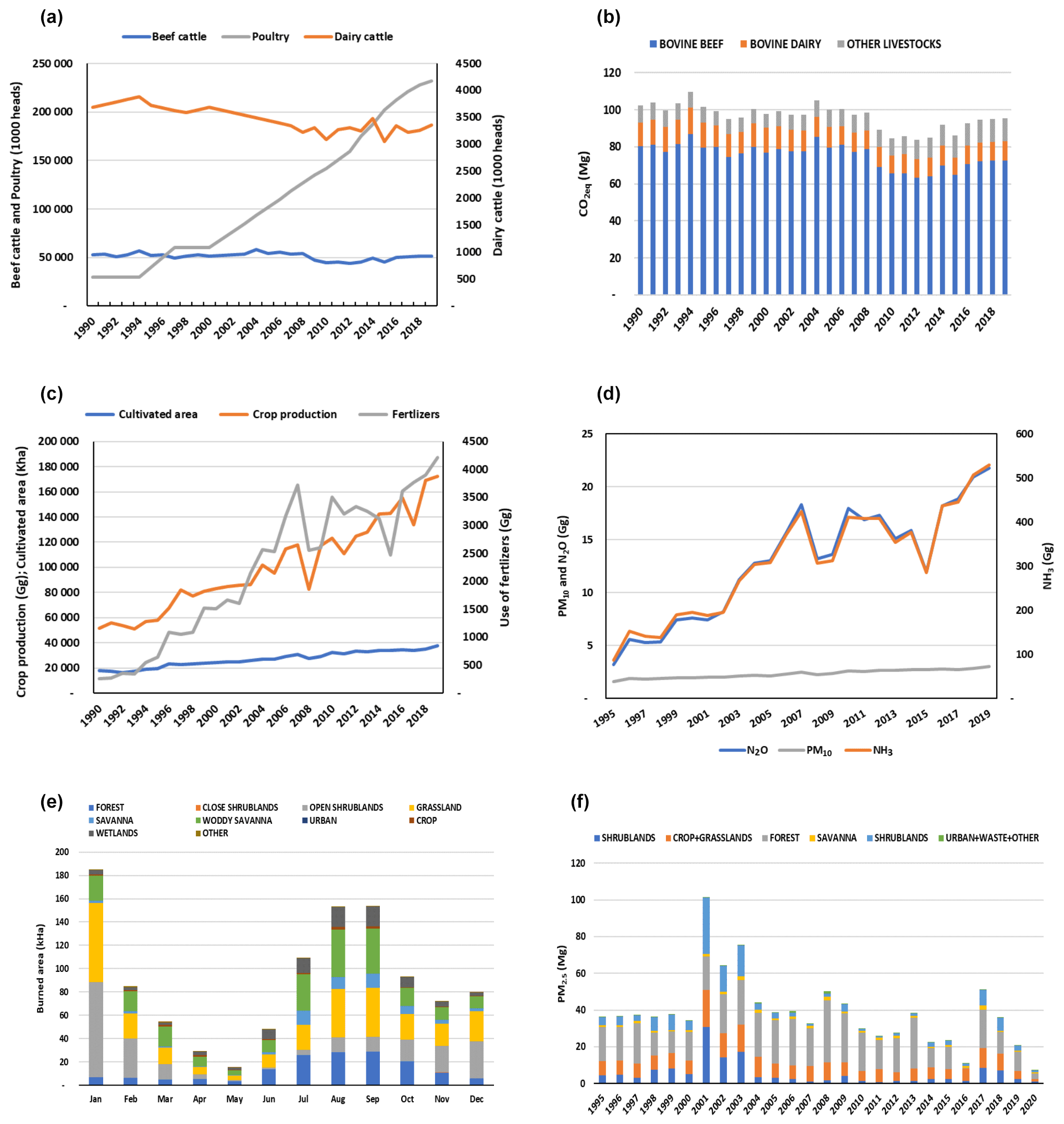
Figure 4(a) Annual animal production for three types of livestock: beef cattle, dairy cattle, and poultry; (b) Annual evolution of GHG (in gigagrams) from for three types: bovine (beef production), bovine (dairy production), other livestock breeds. (c) Annual evolution of main agriculture indices: crop production (Gg), cultivated area (kHa), and use of fertilizers (Gg). (d) Annual emissions of N2O, NH3, and PM10 from fertilizer use and arable lands. (e) Average station burned area in kilohectares for the period 1995–2020, according to land type. (f) Annual emissions evolution of PM2.5 (kt) for the period 1995–2020, according to land type.
The production of cereals and other crops is also known annually, by type of crop within each department. The annual quantity of used fertilizers is also known by type of crop. The spatial distribution of the cultivated hectares by type of crop was made using a land use map, distributing in each department the cultivated area and type of crop in agriculturally available land. The monthly emissions were simply estimated as proportional to 1/12 of the annual value since the monthly distribution was not available.
2.3.7 Burning of agricultural residues and open fires
For the location of biomass burning, crop residue burning, and other biomass fires (natural and/or man-made), we used the MCD64 collection C6 of the MODerate resolution Imaging Spectroradiometer (MODIS) sensor, aboard the (MOD14) Terra and (MYD14) Aqua satellites (Giglio et al., 2009, 2013), between 2001 and 2020. From years 1995 to 2000 we used information from national fire statistics (Environmental Ministry, https://www.argentina.gob.ar/ambiente/fuego/alertatemprana/reportediario, last access: 8 October 2021; CONAE, https://www.argentina.gob.ar/ciencia/conae/aplicaciones-de-la-informacion-satelital/incendios, last access: 8 October 2021). The MODIS collection provides two types of products: fire points (fire events at a daily basis) and burned area (monthly averages, with percentages corresponding to different land uses). The emissions were estimated using the appropriate emission factor corresponding to the specific land use class of each burned area (Puliafito et al., 2020a).
The present inventory is a multi-dimensional database that embraces spatial coordinates, latitude, and longitude, with a spatial resolution of (1441×921 cells) for the whole continental and maritime Argentine domain, a temporal resolution of 300 months from January 1995 to April 2020, 15 activity sectors, and 12 pollutants. It is, then, possible to think of multiple ways to organize and show the results. Therefore, in this section we will only present some representative figures and tables oriented to compare the absolute and relative contribution of each subsector to the total emission of each species, as well as to highlight the spatial and temporal variability for the whole country and within different regions. Note that the whole database has been published for its use in air quality/climate model applications in a standardized format within a free-access repository as indicated in the Data availability statement. Figures 3 to 6 show selected sectors and species distribution. Figures 7 to 9 cover the results of comparing GEAA with other commonly used inventories.
The appendices and Supplement provide the monthly and annual emission time series, as well as basic representative figures.
3.1 Electricity production sector
As of December 2019, Argentina had a total installed capacity of 39 704 MW, where 64.3 % (25 547 MW) corresponded to sources of thermal origin, 28.5 % (11 310 MW) to hydro, 5.3 % to renewable (2092 MW: 1609 MW wind, 439 MW solar, and 42 MW biogas: 2 MW), and 4.4 % (1755 MW) to nuclear. In 2019 annual thermal generation reached 80 137 GWh, hydraulic reached 35 370 GWh, nuclear reached 7927 GWh, and renewables reached 7812 GWh. Figure 2a shows the spatial location of thermal power plants in Argentina. Annual thermal generation for 2019 was produced using mostly natural gas (17 209 200 cubic meters), diesel (403 800 cubic meters), fuel oil (185.6 Gg), and mineral coal (221.8 Gg), with an average efficiency of 1858 kcal kWh−1. Figure 3a shows the total energy consumed at TPP according to the type of generation. The GHG emissions variation, in terms of CO2 eq. (GWP100: CO2=1; CH4=25; N2O=298) (Myhre et al., 2013), is shown in Fig. 3b and Table 3. The monthly evolution for several pollutants is shown in Fig. A2a. The large variations in these emissions were associated with three important variables. (a) There was a low-frequency variation (with a maximum between May 2015 and May 2017 and minimum in December 2002), corresponding to the economic activity that impacts generation and fuel consumption. (b) There was a variation of medium frequency, corresponding to the seasonal summer–winter variation, which depends on the ambient temperature, with heavy consumption in the summer months, for example, due to the use of air conditioning. (c) There was a third variation of greater frequency associated with the type of fuel. An increasing proportion of natural gas use and a decrease in gas oil and coal are shown in Fig. S3 in the Supplement. These have been reinforced in recent years due to increased natural gas production from the Vaca-Muerta basin (approx. 38.64∘ S, 69.86∘ W) from non-conventional wells (Minem, 2020; Rystad, 2018). Figure A2b also shows that during austral winter months TSP emissions (and SO2) increased and those of NOx decreased. This is due to the reduction in the use of natural gas (the main residential heating fuel) and an increase in coal and fuel oil in power plants to compensate for the natural gas reduction. In summertime the opposite occurs, larger use of natural gas and a reduction of fuel oil and coal result in higher NOx and lower TSPs. Note that during diurnal high electricity demand (peak hours) the thermal plants may also be covered by fuel oil and gas oil. In terms of GHGs, emissions from electricity production have steadily climbed around 2 % per decade, from 7.1 % in 1995 (with respect to total annual – all sectors) to 11.7 % in 2019. NOx values have increased from 10.2 % to 14.5 % (with respect to total annual – all sectors) during the same period.
Table 3Summary of annual emissions for 2019 and 1995 for Argentina.
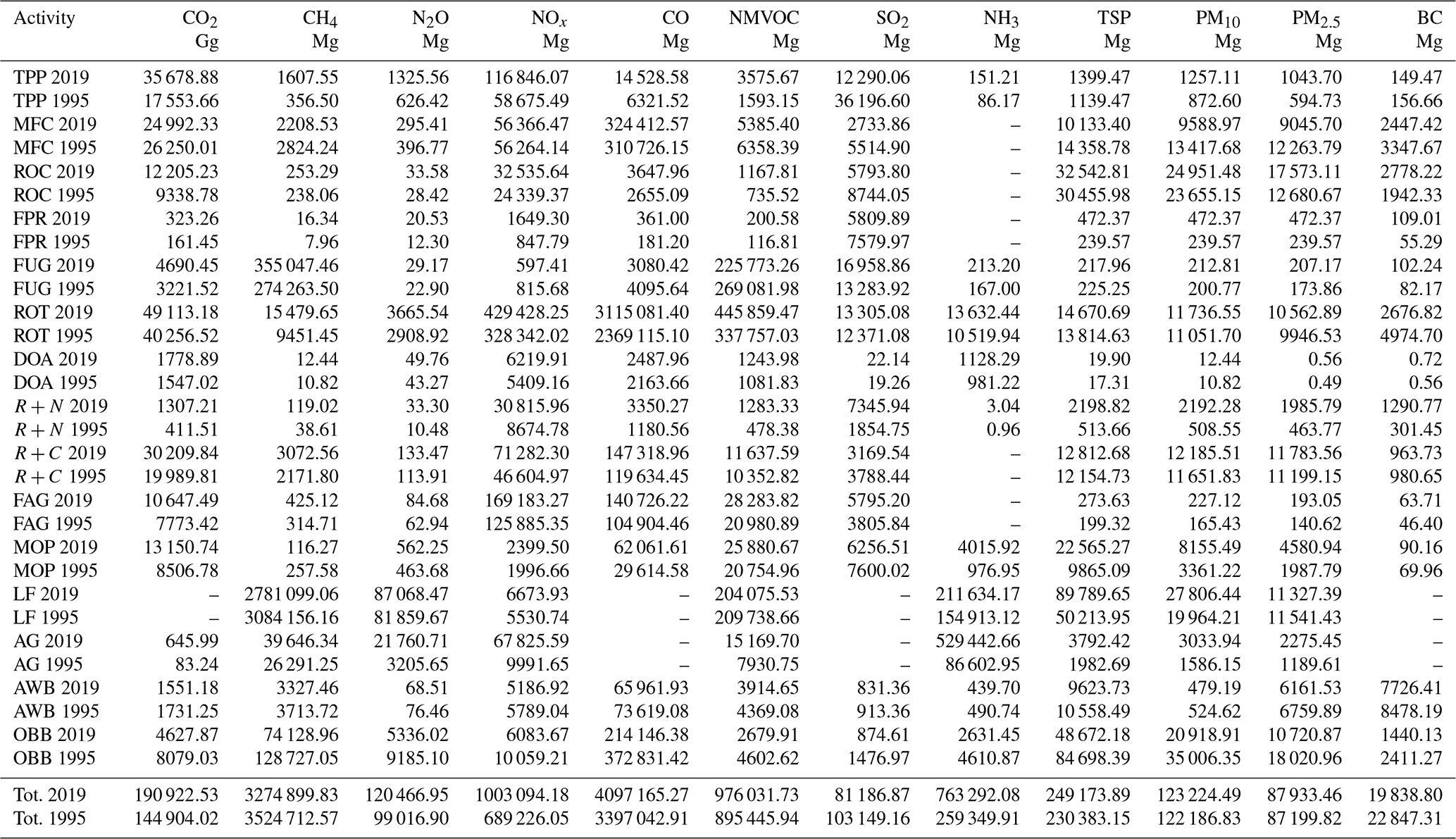
Ref: (see Table 1a): TPP: power plants; MFC: manufacturing's own fuel consumption; ROC: refinery consumption; FPR: fuel production; FUG: fugitive, venting, and flaring; ROT: road transport; DOA: domestic aviation; R+N: railroad and navigation; R+C: residential and commercial; FAG: fuel use in agriculture; MOP: manufacturing's own process; LF: livestock feeding; AG: agriculture; AWB: agriculture waste burning; OBB: open biomass burning.
3.2 Fuel production sector
Emissions from fuel production correspond to refineries' own consumption (ROC), and extraction wells, for their own operation of the activity and transformation (FPR). Fugitive emissions from venting or flaring of surplus gas are also included in the refineries and wells sector (FUG). Figure A2d shows the monthly variation between the years 1995 and 2020 of methane emissions, reaching a monthly average of 28 117±3382 Mg per month for the three activities. However, the total CH4 emission is dominated by the refinery venting and flare activity. The increase after November 2018 is mainly due to a growth in the production of unconventional natural gas in the Vaca-Muerta basin in the last 2 years (Fig. A2c). Figures S6 and S7 also shows the activity and emissions of the extractive activity of gas and oil (up-stream) at wells from their own consumption. Monthly GHG emissions () have increased from 2315.62 Gg CO2eq in December 1995 until reaching 3344.28 Gg in December 2019. Table 3 show the total annual emissions for oil and gas production for all pollutants considered. Fuel production and transformation () represented 11 % in 1995 % and 13 % in 2019 of total annual GHGs considered. Pollutants such as CO and NOx have an annual contribution share of 0.2 % and 3.8 %, respectively, for the year 1995 and 0.2 % and 3.5 % for the year 2019, respectively (Table 3 and Fig. 5).
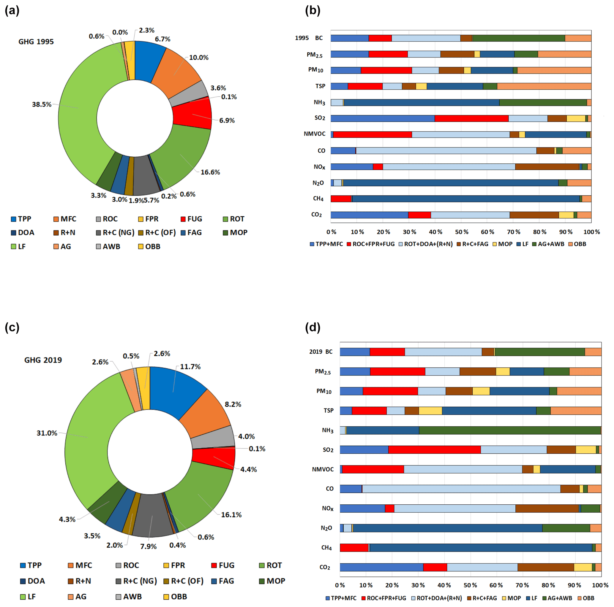
Figure 5GHG participation by activity for Argentina for the years 1995 (a) and 2019 (c) (see Table 3) and sectoral SLCP pollutant contribution share of emissions for Argentina: (b) 1995 and (d) year 2019. Reference codes are provided in Table 1a.
3.3 Transport sector
Figure A1c shows the monthly country fuel sales variation for the main fuels used in the road-transport sector (ROT) from January 1995 to December 2019. Figure A1d presents the total monthly emissions of CO, NOx, and PM10 from the same activity. Table A4 shows a growth of 13 % in the period from December 1995 to December 2019 for CO2 and CO2eq, 54 % for methane, 21 % for NOx, and 20 % for CO and NMVOC for the same period. The main growth is due to the higher consumption of gasoline while diesel oil has only grown slightly and compressed natural gas (CNG) has remained stable. However, similarly to the energy production sector, fuel consumption is strongly linked to economic activity (i.e., represented by the gross domestic product (GDP) as we will discuss later in Sect. 3.7), showing decreasing consumption from 1995 to 2002, and then climbing again. From August 2016 and on, a stagnation in gasoline consumption appears, in accordance with a retraction in national economic activity. Figures A1c and d also show a 52 % and 63 % reduction in NOx and CO ROT emissions, respectively (comparing April 2020 with respect to April 2019), due to the COVID-19 quarantine effect (which began on 20 March 2020, Table A5; Bolaño-Ortiz et al., 2020). Additionally, Fig. S8 includes monthly and annual GHG emissions (CO2, CH4, and N2O) and SLCP (BC, CO, NMVOC, NOx, SO2, NH3) from road transport. Regarding domestic aviation (DOA), Fig. A2e shows monthly fuel consumption (m3) from LTO, while Fig. A2f shows the respective monthly emissions (CO2, CH4, N2O, NOx, CO, NMVOC, SO2 NH3, TSPs, and PM). The aviation activity has been relatively stable with an increasing trend since the year 2005. The year 2020 had a complete stop due to COVID-19 restrictions, only partially re-establishing after November 2020.
Figure A3 shows the active railroad network (Fig. A3a); the average seasonal variability in RR activity (Fig. A3b), in terms of tkm for freight and passenger kilometers for transported passengers; and the monthly fuel consumption and number of transported passengers (Fig. A3c). The passenger activity is mainly Buenos Aires commuting activity (>95 %). With respect to fuel consumption (gas oil), RR freight activity represents on average 45 %, and it is expected to increase as crop production and export increases. Note that following the agriculture exportation, freight RR shows a marked seasonality, where the maximum austral winter activity (June–July) is up to 40 % higher than during the summer (January–February). The inter-annual increase is also seen in inland navigation since ports like Rosario, Santa Fe, and Bahía Blanca are hubs for the soybean, wheat, and maize export. Both railroad and inland navigation activity have shown an increase of 122 % in pollutant emissions since December 1995 with respect to December 2019.
3.4 Residential, commercial, and governmental sector
Residential, commercial, and government (R+C) energy consumption includes electricity (for lighting, air conditioning, and partially heating) and natural gas for cooking and heating in a large part of the country (except for northeast Argentina; see Fig. A3). For urban areas not connected to the natural gas (NG) network, the heating energy consumption is replaced by electricity, LPG, and kerosene; in rural areas with abundant biomass available (northeast of the country), charcoal and wood are used. According to data from radio maps and census fractions, there are 12 171 560 homes in Argentina (INDEC, 2020), of which 56 % are connected to the NG network, 41 % use LPG, and the remaining 3 % use wood, charcoal, or kerosene. The 2019 annual consumption reached 10 680 070 (1000 m3) of NG, 855 184 (1000 m3) of LPG, 285 113 Mg of wood, 341 473 Mg of kerosene, and 484 408 Mg of coal. The annual average per capita consumption is 268 m3 of NG, 21.38 m3 of LPG, 12.11 kg of charcoal, 7.1 kg of firewood, and 8.5 kg of kerosene. Figure 3c shows that the annual fuel consumption of wood and LPG has decreased since 2001 and 2007, respectively, compensated for by a gradual increase in the consumption of NG since 1995. Note that the residential fuel consumption shows a very strong seasonal and regional cycle (Figs. 3d and A3) due to the large north–south extension of Argentine territory. For the year 2019, NG use represents 80 % of the total R+C annual emissions for CO2, 14 % for CH4, 91 % for NOx, 15 % for CO, and 7 % for TSPs; also, the use of other fuels contributes 93 % of PM10 and 85 % of CO (Tables 3, A4, and A5). Emissions from R+C electricity using fossil fuels are considered in the thermal power plant sector.
3.5 Industrial sector
This subsection includes the monthly emissions from industrial manufacturing's own fuel consumption (MFC) and emission from the production process (MOP) from January 1995 to April 2020. Note that manufacturing electricity consumption is considered in the thermal power plant sector. Table A3 shows a list of the manufacturing activities considered, whereas Fig. 2b shows the location of the manufacturer sector. The monthly fuel consumption averages are 846 380 (1000 m3) of natural gas, blast-furnace gas, and coke-oven gas together; 13 493 Mg of LPG; 36 234 Mg of gas oil, diesel oil, and fuel oil; and 668 374 Mg of coal wood and biomass. Natural gas is used as industry's own main fuel consumption followed by wood and crop residues, with the latter especially used in the food elaboration subsector, like sugar, paper, and wood production, due to local availability of biomass. Seasonal fluctuations, in both consumption and emissions, are due to variations in production, but they are also conditioned by less availability of natural gas during the winter months, which is due to residential consumption. Monthly average GHGs from industry's own fuel consumption reached 2405.23 Gg per month of CO2eq, while for NOx consumption reached 5 053.27 Mg, 28 861.79 Mg for CO, and 1250.46 Mg for TSPs.
The MOP included the emissions from the manufacturing's own production process and included the following subsectors: 2A glass production; 2B chemistry; 2C aluminum steel; 2D asphalt, painting; and 2H paper, food, beverage. Figure 3e and f show the annual evolution of MOP NOx and PM10 emissions. The chemical industry contributes to 37.1 % of NOx emissions, followed by the food industry with 36.5 % and the steel industry with 26.4 % with respect to total MOP emissions. For PM10 emissions, the cement industry contributes 35.0 %, the chemical industry contributes 22.2 %, the steel industry contributes 20.6 %, the food industry contributes 20.4 %, and automotive painting contributes 1.8 %.
3.6 Agricultural and livestock sector
Emissions from the agricultural livestock sector were calculated annually from 1990 to 2019. Emissions from livestock included enteric fermentation (CH4) and manure management (CH4, NO2, NH3, NOx, NMVOC, and PM). These emissions depend on the type of animal, age, type of production, and productive areas. In terms of methane emissions (i.e., CO2eq), the bovine sector dominates Argentina's GHG emissions (31 %), reaching 95 473 Gg CO2eq in 2019 (2781.09 Gg CH4; 87.09 Gg N2O). The historical series shows an average of 96 301 Gg CO2eq between 1995 and 2019 for all livestock production (Fig. 4b), with a slight decrease in 2009 caused by a reduction in bovine animal production. Total animal production has grown from 177 million head in 1990 to 317 million head in 2019. While bovine livestock has oscillated between 54.7±3.4 million head, the largest increase was in the poultry sector, from 30 million birds in 1990 to 232.3 million in 2019, producing a significant increase in ammonia emissions (from 6.6 Gg NH3 in 1990 to 51.1 Gg in 2019; see Fig. 4a). Total ammonia emissions in 2019 reached 211.63 Gg for all livestock.
Emissions from the agricultural sector are characterized by a strong increase in cultivated area, increased production, and increased use of fertilizers (Fig. 4c). Considering the period from 1990 to 2019, these numbers more than doubled from 17 700 to 37 873 kHa in cultivated areas; approximately tripled from 51 457 to 172 089 Gg for cereal production; and increased at least by a factor of 15 (from 260 to 4217 Gg) for fertilizer use. As a consequence of this increase in fertilizers, the largest emissions increases were for ammonia and nitrous oxide, which changed from 38.09 Mg in 1990 to 529.44 Mg in 2019 for NH3 and from 1.58 Mg in 1990 to 21.76 Mg in 2019 for N2O (Fig. 4d).
3.7 Burning of agricultural residues and fires
For this sector, accidental and/or provoked fires from biomass burning were considered, from both agricultural residues and other types of fires between 1995 and 2020. Figure 4e shows an average seasonal burned area according to main land types, and Fig. 4f shows the evolution of PM2.5 (Gg) emissions for the period 1995–2020, according to land type. Figure A5b shows the monthly average precipitation (1981–2018), calculated using the Climate Hazards Group Infrared Precipitations with Stations (CHIRP) database (Funk et al., 2015; Rivera et al., 2018). It clearly shows the correspondence with the land use map (Fig. A5a) and directly with the availability of ground fuel from biomass. Figure A5c shows the average monthly burned area (2001–2020), which shows two distinct areas: northeast (rain>50 mm per month) and the semi-arid (rain>20–50 mm per month) central-west zone of Argentina. In the northeastern area of Argentina fires predominate between August and November, associated with burning of crop residues and land changes (clearing forest for agriculture), while in the central west of the country fire events increase during the summer months (December and January) on dry grasslands and pastures. These fires are associated with typical dry conditions in the previous winter and spring months before the rainy season begins in late summer (February and March). Figure A5c shows the emission of PM2.5 associated with burning of biomass.
According to land type use considering the 1995–2020 period, annual burned area averages 1 064 423 Ha, with 14.7 % forest, 27.1 % grassland, 25.6 % savanna, 22.0 % shrublands, 7.7 % cultivated areas, and the remaining 2.9 % corresponding to other types of land use.
3.8 Summary and discussions of GEAA-AEIv3.0M results
Table 3 summarizes the total annual emissions for the years 1995 and 2019, while Table A4 presents a single timeframe with the monthly emissions for December 1995 and December 2019. From the point of view of the GHG emissions, the main emission sector is livestock (38.5 % and 31 % for 1995 and 2019, respectively), showing a 7.7 % reduction trend due to decreasing bovine production (see Fig. 5). Adding together thermal power plants' and manufacturing's own fuel production represents 16.8 % and 19.9 % of the total GHG emissions (for 1995 and 2019, respectively), followed by 16.6 % and 16.1 % for road transport (1995 and 2019, respectively). The residential plus commercial sectors have increased from 7.6 % to 9.8 % for the above-referenced years. This is consistent with population increase, as analyzed below. In absolute values GHGs have increased from 263 391 Gg CO2eq in 1995 to 307 707 Gg CO2eq in 2019 (17.5 % increase with respect to 1995). Note that the GEAA-AEIv3.0M GHG inventory does not include land use changes nor sewage waste, since its focused on air quality, and therefore these are not the total GHG numbers for Argentina; in fact, TCNA (2015) reports total CO2eq of 368.295 Gg for the year 2014. Most notably, the main increases are observed for NH3 and N2O emissions due to the use of fertilizers in agriculture (Fig. 4d). Indeed, Argentina has increased its annual crop production from 51 735 to 172 089 Gg and annual use of fertilizers from 641 to 4217 Gg (1995 and 2019, respectively), while bovine production has decayed slightly from 55 921 in 1995 to 54 698 head in 2019 (Fig. 4a). From a climate change perspective, reducing N2O emissions through reducing crop production is a critical economic option, since together with livestock feeding, both activities represent the main export income for Argentina. Thus, it is not expected that the percentage contribution of N2O to Argentine GHGs will be reduced until new nitrogen-use efficiency of crops could be incorporated worldwide to reduce emissions (Solomon et al., 2020; UNEP, 2013).
Air quality SLCP sectorial shares are shown in Fig. 5b and d for 1995 and 2019, respectively (see also Table 3). Comparing those two years for a particular pollutant, e.g., CO, shows that the dominant sectors contributing to the total emissions remain unaltered and present only minor percentage changes: road transport is the most important sector, representing 69.7 % and 76.0 % for the years 1995 and 2019, respectively, followed by open fires (11.0 % and 5.2 %) and burning of agricultural residues (2.2 % and 1.6 %, for the years 1995 and 2019, respectively). Similarly, NOx emissions are concentrated in road transport activity, 47.6 % and 42.8 %; thermal power plants' and manufacturing's own fuel production contribute 16.7 % and 17.3 %; and residential and commercial contributed 6.8 % and 7.1 % (1995–2019, respectively). Fire and biomass burning represent the largest source of particulate matter (TSP) (41.3 % and 23.4 % for the years 1995–2019, respectively) coming from agricultural waste, clearing forest for agriculture and livestock feeding, and natural burning of grassland. Nevertheless, it should be noted that the TSP contribution from different sectors is highly variable from year to year (Fig. 4f).
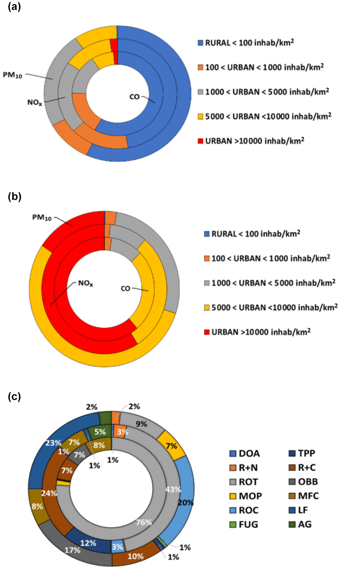
Figure 6Annual PM10 (outer ring), NOx (middle ring), and CO (inner ring) emissions distribution according to different classifications: (a) total emissions with respect to population density, (b) emissions density () with respect to urban density, (c) total sectoral contribution (see Table 4). Reference codes are provided in Table 1a.
Table 4Emission distribution of CO and NOx according to population density for the year 2019.
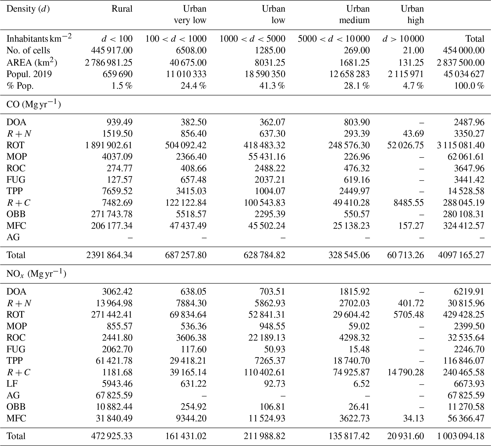
The total Argentine population, surface extension, total emission, and emission density are classified according to the mean urban density within each cell. Ref: (see Table 1a): PP: power plants; MFC: manufacturing's own fuel consumption; ROC: refinery consumption; FPR: fuel production; FUG: fugitive, venting, and flaring; ROT: road transport; DOA: domestic aviation; R+N: railroad and navigation; R+C (NG): residential and commercial (natural gas); R+C (OF): residential and commercial (other fuels); FAG: fuel use in agriculture; MOP: manufacturing's own process; LF: livestock feeding; AG: agriculture; AWB: agriculture waste burning; OBB: open biomass burning.
The three concentric rings presented in Fig. 6 summarize the sectorial contribution to the main primary air quality pollutants (see also Table 4): the outer ring is for PM10, the middle ring for NOx, and the inner ring for CO. Figure 6a shows the proportion of total annual emissions with respect to urban population density. A total of 57.0 % of PM10 emissions (70 189 Mg), 47.1 % of total NOx emissions (472 925 Mg), and 58.4 % of total CO (2 391 864 Mg) are emitted in areas with low urban density (<100 inhabitants km−2), since many roads and thermal power plants are in these locations, and Argentina has a vast non-urbanized area (see Table 4). Note that 25.9 % of Argentina's population lives in towns with fewer than 1000 inhabitants km−2, 69.4 % in urban centers with between 1000 and 10 000 inhabitants km−2, and 4.7 % in dense urban centers with greater than 10 000 inhabitants km−2. Air quality in urban areas is dominated by road transport, residential and commercial emissions, and depending on the cities also power plants and industrial energy consumption and production. For example, for NOx, the population is exposed to average daily emissions of 0.5, 10.9, 72.3, 221.3, and 436.9 for ≤100, >100 and ≤1000, >1000 and ≤5000, >5000 and ≤10 000, and >10 000 inhabitants km−2, respectively. However SLCP high emissions density per squared kilometer is emitted in the denser urban area (>10 000 inhabitants km−2): 1998 for PM10, 159 479 for NOx, and 462 577 for CO (Fig. 6b), resulting in those urban regions possessing lower air quality standards than rural areas. Figure 6c shows the proportion of the same SLCP (PM10, NOx, and CO) but as a function of the sectors. These figures show that although CO and NOx have the highest emissions density in urban centers and are dominated by road transport and power plants, maximum PM10 is located in medium-density areas (6990 at urban density of ) and are dominated by residential and road emissions. Nevertheless, in absolute numbers PM is dominated by fire produced in agriculture and forest areas, livestock feeding, and refineries.
The evolution of GHG and SLCP air pollutant emissions clearly shows a strong dependence on population increase and gross domestic product (GDP) changes. Figures A6 shows a normalized quarterly series of GDP, de-trended population and GHG. While population follows a linear trend (0.04 % quarterly increase), GDP has a 6–8-year oscillation over the population increases, presenting local minima for October 2002 and April 2020, and local maxima for April 1998 and April 2013. GHG variation follows the GDP changes with an extra annual seasonal variation. Note that the medium-term 6–8-year oscillation and the annual seasonality are appreciable in the use of fossil fuels for electricity production, as described in Sect. 3.2. Finally, Fig. A6c shows the GHG/cap and GHG/GDP variations, whose trends are followed by the emission of many other pollutants (not shown). Several conclusions may be extracted from the above results. First, GHG and air quality pollutants mainly follow population increase modulated by economic activity, where Argentina's recurrent economic crises are very visible in these time series. Second, GDP has fallen below population increases since 2019, aggravated by the COVID-19 lockdown crisis in 2020 (Bolaño-Ortiz et al. (2020); see Table A5 for monthly values for April 2019 and April 2020). Third, quarterly GHG/cap has been stable at 639±65 kg per capita during the whole period, which means there has there been no major enhancements in personal consumptions, but neither have been any improvement in the emissions efficiency. Fourth, GHG and GDP show a quarterly variability of 51±21 g per US dollar, showing a slight decreasing trend from 2004 to present, since less carbon is emitted per expended US dollar, most probably due to technological changes (note that the sudden increase in 2002 is produced by the reduction of GDP during the 2001–2002 economic crisis). Fifth, approximately one-third of GHG emissions come from agriculture and livestock emissions, main export activities of Argentina. Another third arises from energy production (TPP) and transport (), and the remaining third comes from the other sectors. Sixth, GHGs are still coupled to GDP (and population), which means that reducing GHG emissions in Argentina can only be done, at present, at the expense of reducing activity intensity (i.e., reducing economy), as is clearly seen in 2020 reduction due to lockdown because of COVID-19. Seventh, air pollution in urban cities is mainly produced by road transport (i.e., CO, NOx, and PM2.5) and power plants (SO2 and NOx), and even though the largest emission densities are in large urban areas, due to the vast majority of rural areas in Argentine territory, the total national emissions originate in the less populated regions.
Since the present GEAA-AEIv3.0M inventory includes spatial and temporal variation, its calibration requires a double control and validation. For the temporal comparison we use the Argentina national greenhouse gas inventory (TCNA, 2015) that compiled the total annual values for Argentina between 1990 and 2014 and an updated version in 2019 (TCNA, 2019) spanning from 1990 to 2016 as well as the international inventories EDGAR HTAPv5.0 and CEDS. It should be noted that CEDS uses TCNA 2015 as a basis for the Argentine information (Hoesly et al., 2018), but for some species and sectors they differ slightly. There are also some differences between TCNA 2015 and TCNA 2019. Therefore, we will compare GEAA with four temporal series: TCNA2019, TCNA2015, CEDS, and EDGAR.
Although the activity data for both studies for GEAA and TCNA (and CEDS) were basically taken from the same national sources (mostly from the National Energy Balance), the focus and methodology of each inventory vary. In TCNA, activities and emissions are accumulated using a top-down approach to obtain a nationwide annual total by sector. In our case (GEAA-AEIv3.0M) the activities and emissions are first located in each point, line, or area with a bottom-up approach, and then the totals are calculated as the sum of all cells in the spatial grid. Therefore, the sum of the activities by sector and year may vary. With respect to EDGAR, the sum differs in particular in the use of proxy variables used for its spatial disaggregation, which has already been discussed elsewhere (Puliafito et al., 2015, 2017). A spatial comparison can also be made with the EDGAR inventory presented in Sect. 4.2.
When comparing with other inventories, emphasis has been placed on greenhouse gases (GHGs), since GHGs relate to the level of agreement (or discrepancy) with the activities of each sector, since their emission factors (EF-GHG) are well established and are especially associated with energy consumption (Sato et al., 2019). On the other hand, air quality emission factors (EF-AQ, those used for NOx, CO, PM, and others) are highly variable, mainly due to uncertainties in the environmental and technological conditions considered for each activity. For example, for an on-road vehicle, the emission factors will depend on the outside temperature, engine temperature, type, and quality of fuel, idle or regime status, slope, load, and age, among other factors (EMEP, 2019). Thus, the used average EF-AQ will include a mixed weighted operational condition. In the same line, although electric vehicles have EF-AQ=0, EF-GHG will still depend on how the consumed electrical energy is generated.
4.1 Comparison with total annual values from TCNA, EDGAR, and CEDS
Tables 5 and A7 summarize the total annual values for GHG emissions (CO2eq Mg) for GEAA-AEIv3.0M and TCNA 2015 inventories, respectively. Note that the original TCNA report included contributions from other sectors (land use changes) not related to air quality that are not considered here.
Table 5GEAA-AEIv3.0M inventory: annual GHG emissions values (CO2eq Gg) for Argentina.
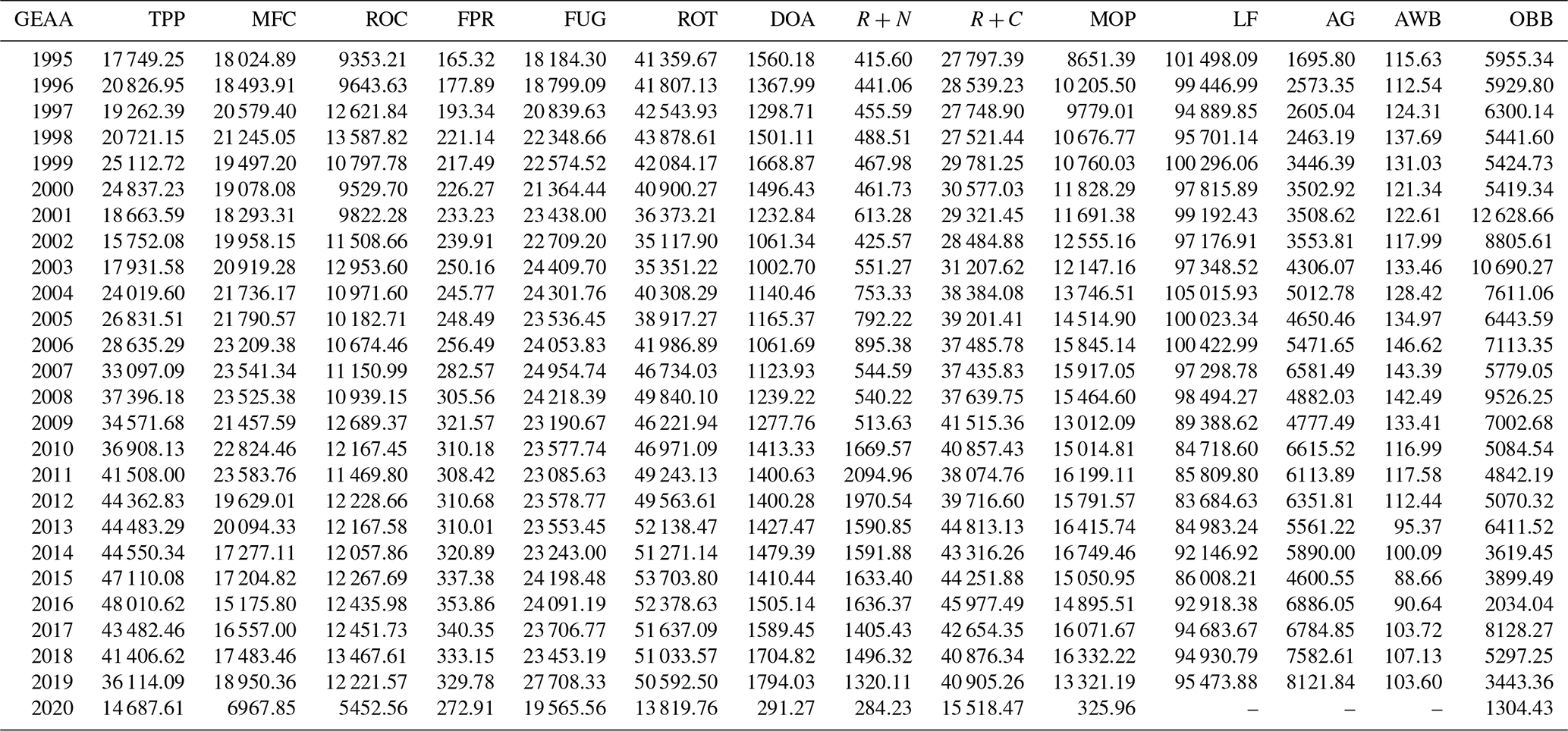
Ref: (Table 1a) TPP: power plants; MFC: manufacturing's own fuel consumption; ROC: refinery consumption; FPR: fuel production; FUG: fugitive, venting, and flaring; ROT: road transport; DOA: domestic aviation; R+N: railroad and navigation; R+C: residential and commercial and others; MOP: manufacturing's own process; LF: livestock feeding; AG: agriculture; AWB: agriculture waste burning; OBB: open biomass burning.
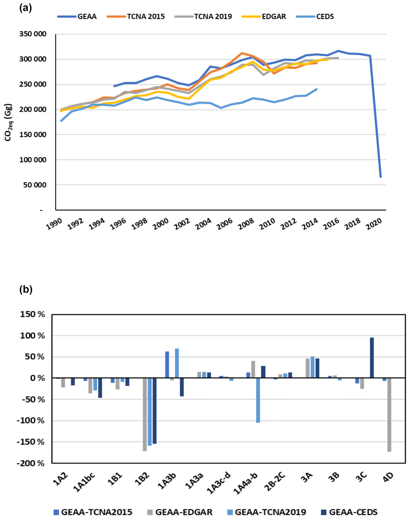
Figure 7(a) Evolution of total annual CO2eq Gg emissions for the GEAA (red), TCNA2015 (blue), TCNA2019 (light-blue), EDGAR (green), and CEDS (brown) inventories for Argentina in 1990–2019 (Tables 5 and A5). (b) Percentage difference in GHG emissions () for 1995 through 2016, for the considered activities (see also Tables A7 and A8). Note that CEDS does not provides N2O profiles. GHGs are calculated as .
Figure 7a shows the annual values for the TCNA2019, TCNA2015, CEDS, and EDGAR inventories, and Fig. 7b shows the average annual differences by activity. In the Supplement (file comp_geaa_ceds_edgar_tcna.xlsx; see the Supplement for description) we present a sectorial comparison for CO2, CH4, N2O, CO, NOx, SO2, and NMVOC among the TCNA2019, TCNA2015, CEDS, and EDGAR inventories. Table A7 summarizes the main results for the inventory intercomparisons. Most of the activities (1A1, 1A2, 1A1bc, 1A3a, 1A3b, 1A4abc, 2B, 2C, 3A, 3B; see Table 1a) agree within ±27.0 % for all inventories and the considered pollutants.
CO2eq in GEAA and TCNA2015 agree for the sum of all sectors within 7.1 % (Table A9). Higher discrepancies between GEAA and TCNA are found in N2O profiles, and sectors 1B2 (FUG>60 %), 1A3c-d (R+N: 13.3 %), and 3C (AG: −12.5 % and AWB: −6.5 %). For fuel production, the discrepancy arises from the way the activity is computed. In the public energy 1A1a sector, GEAA and TCNA agree within 1.5 %, while EDGAR and CEDS have 16 % larger CO2 emissions and 95 % higher values for CH4. For NOx, CO, SO2, and NMVOC all profiles (GEAA-AVERAGE) agree within 10 %, 32 %, 10 %, and 23 %, respectively. For refinery consumption (1A1bc), manufacturing's own fuel consumption (1A2), all inventories and pollutants' profiles agree within 15 %, but CH4 for 1A1bc has larger dispersion (GEAA-AVERAGE: 45 %). EDGAR also shows high discrepancies for CH4, CO, and SO2 for these sectors (>60 %). Transport (1A3: ROT, DOA, R+N) and residential, commercial, and other (1A4) sectors also have good agreement within 20 % for all inventories and most pollutants. CO profiles from EDGAR show the highest differences (59 %) for 1A4 stor while CEDS presents 21 % disagreement with the mean of all five profiles. Fugitive emissions (sector 1B1 and 1B2) present the highest disagreement, in the solid fuel transformation (coal) and oil–gas production and transformation. GEAA, TCNA2015, and TCNA209 agree within 20 %; CEDS and EDGAR are more than 100 % higher for CH4 and CO than GEAA. EDGAR has 2.5 times more CH4 emissions for the fuel production sectors (1A1bc,1B1,1B2) than GEAA and TCNA (see additional discussion below)
The methane emissions from fuel production and fugitive emissions from oil and gas wells need a deeper study since a bottom-up calculation from each possible source requires in situ/airborne measurements to detect possible leakages from local facilities (Allen et al., 2013; Roscioli et al., 2015; Zavala-Araiza et al., 2014). New high-resolution satellites promise new detection capabilities (i.e., GHGSat. https://www.ghgsat.com/our-platforms/iris/, last access: 8 October 2021).
4.2 Comparison with the EDGAR database
Spatial and total annual emissions were compared to the EDGAR emissions inventory (EDGAR HTAP v5.0) for Argentina. In particular, the EDGAR monthly inventory is available only for 2015 (Crippa et al., 2020), which was used to compare the GEAA-AEIv3.0M monthly values. Table A8 shows a summary of the statistics obtained from this comparison. For this purpose, the GEAA-AEIv3.0M inventory was adapted from a 0.025 to 0.1∘ spatial resolution compatible with EDGAR.
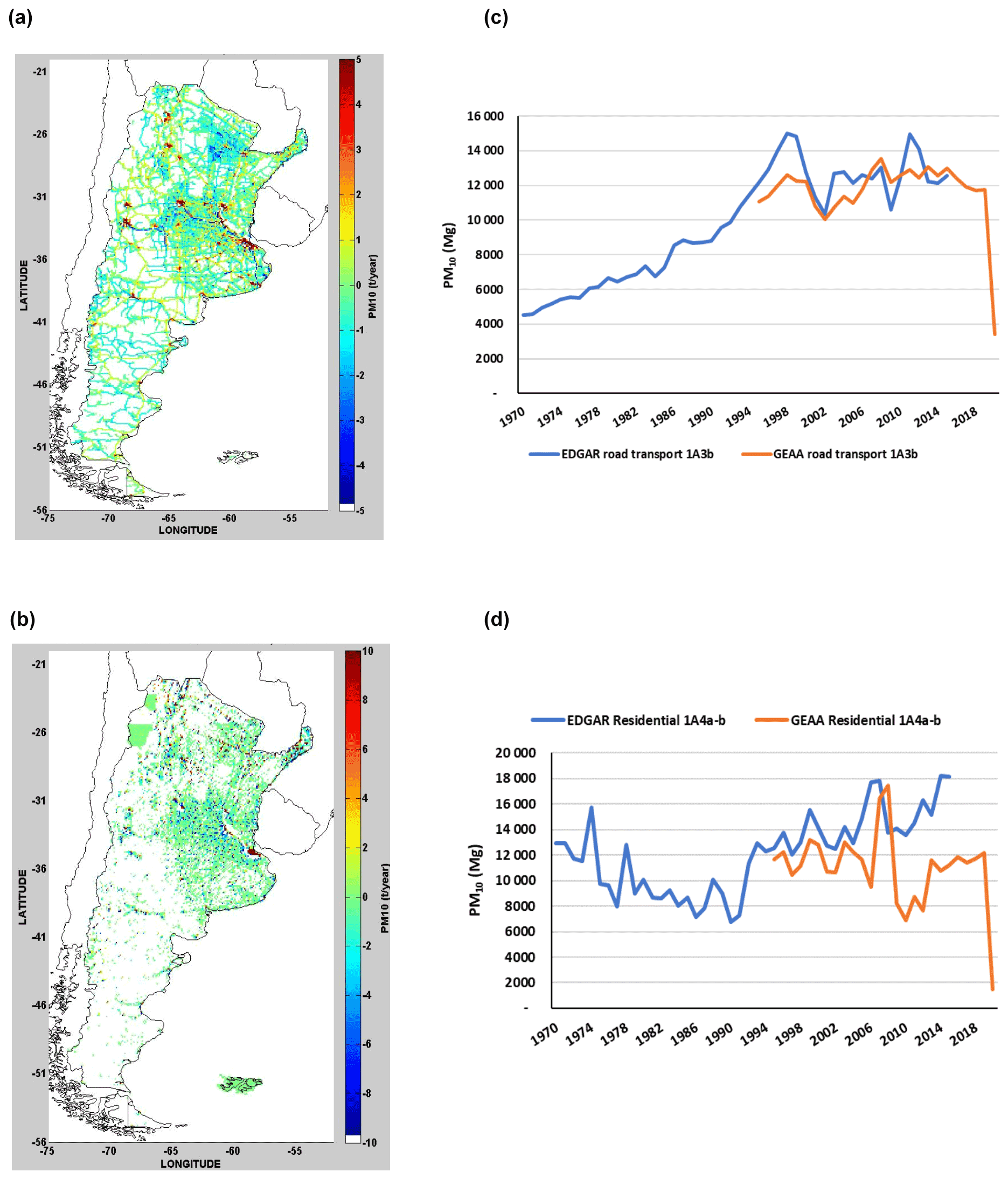
Figure 8GEAA and EDGAR annual PM10 emissions from the road transport sector: (a) differences (t yr−1 per cell) and (c) annual series. GEAA and EDGAR annual PM10 emissions from residential and commercial activities: (b) differences (t yr−1 per cell) and (d) annual series. Maps are represented at 0.1×0.1 resolution for 2015.
Figure 8 shows the annual spatial differences between both inventories for PM10 for the transport sector (Fig. 8a), for the residential and commercial sector (Fig. 8b), and for the annual total evolution for both sectors (Fig. 8c and d, respectively; see also Table A10). Figure 9 shows the same information as Fig. 8 but for NOx.
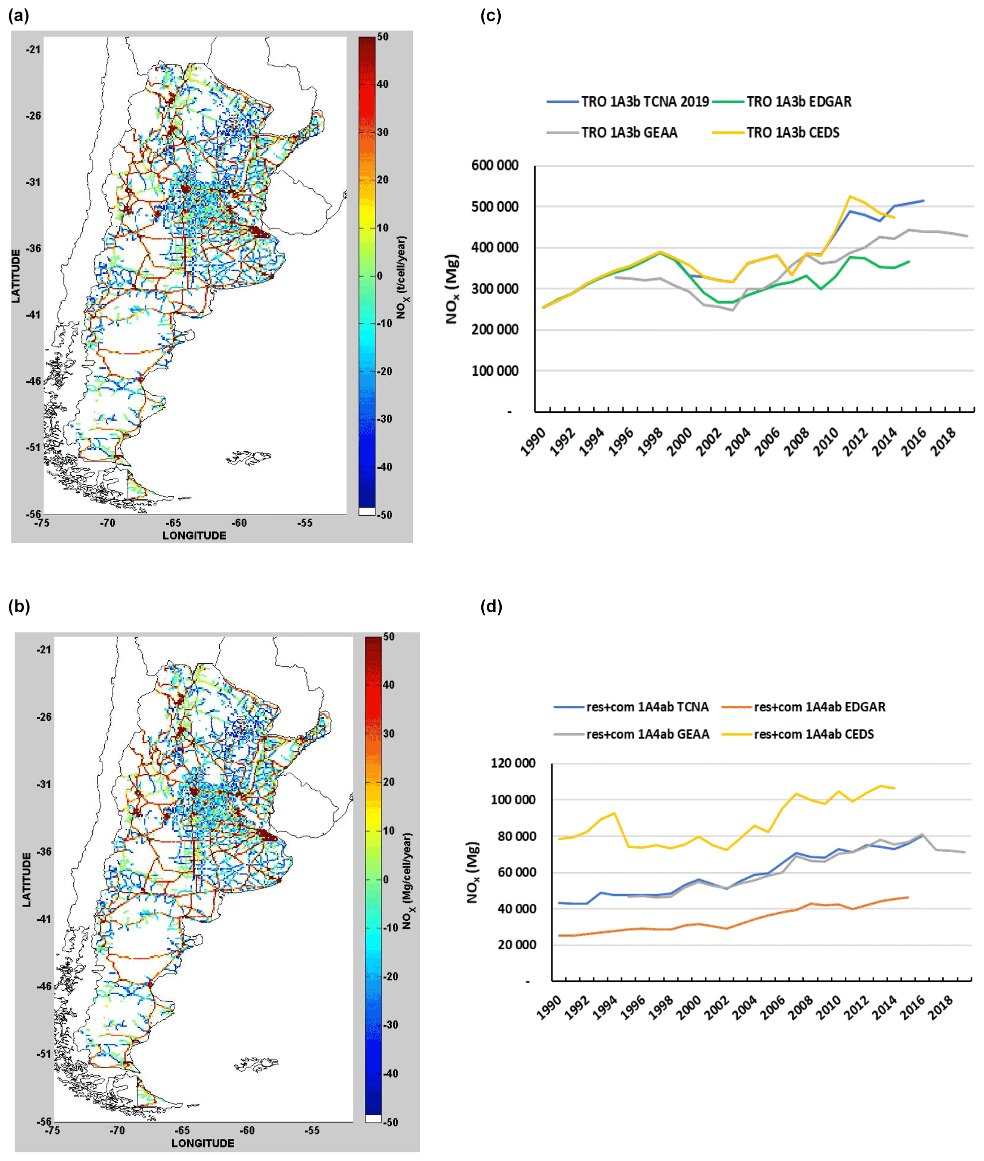
Figure 9GEAA and EDGAR annual NOx emissions from the road transport sector: (a) differences (GEAA-EDGAR; in Mg yr−1 per cell) and (c) annual series. GEAA and EDGAR annual NOx emissions from residential and commercial activities: (b) differences (Mg yr−1 per cell) and (d) annual series. Maps are represented at 0.1×0.1 resolution for 2015. CEDS (light blue) and TCNA (green) profiles are also included for comparison.
The GEAA-AEIv3.0M vs. EDGAR HTAP v5.0 comparison shows several interesting aspects. From the spatial point of view, the residential emissions shown by EDGAR have a distribution based on the districts with surface emissions larger than the properly urbanized area; see for example, green-blue areas in northwest Argentina (Fig. 8b for PM10) which correspond to a mountainous and arid area, with practically no population and only minor industry based on agricultural waste burning. According to Janssens-Maenhout et al. (2019), EDGAR uses national and subnational administrative units as proxy population data using Gridded Population of the World, version 3 (GPWv3) provided by the Center for International Earth Science Information Network (CIESIN, 2005). This approach produces an overestimation compared to the high-resolution population density map in GEAA.
When appreciating the annual values, the differences of PM10 (and other pollutants) show similar values between the years 1995–2008, but thereafter they diverge. Firewood, charcoal, and other primary energy sources used for heating and cooking in homes have been very variable but with a decreasing trend since 2003, being replaced by increasing use of natural gas and LPG (Fig. 3c). While natural gas (NG) represents (on average) 56 % of residential energy, kerosene, charcoal, wood, and other primaries represent only 4 % of energy consumption at households. However, the PM10 emission factor ratio wood NG is 600 to 700, and for NOx wood NG is only 1.2 to 2. Then, any overestimation of wood (and other primaries) will be more visible in PM10 emissions (Fig. 8d) than for NOx (Fig. 9d). As energy consumption inputs, EDGAR uses the International Energy Agency (IEA) World Energy Balances 2016 (Janssens-Maenhout et al., 2019); however wood and other primary energy inputs may have been overestimated, given the high variability, or they might have used a constant per capita consumption. The 40 % higher values of annual residential NOx emissions in GEAA and TCNA (Fig. 9d) with respect to EDGAR are produced by a higher emissions factor adopted in Argentina (TCNA) for NG emissions (150 g GJ−1) compared to 51 g GJ−1 proposed by EMEP (EMEP2019, Sect. 1.A.4b.i., Table 3.3). Had we adopted 51 g GJ−1 as from EMEP, then we would have obtained a lower total of annual NOx emissions, consistent with less primary energy use (firewood, others).
Regarding transport emissions, the spatial distribution differs in the amount of traffic and emissions per route. On the EDGAR map, equivalent emissions have been attributed to primary and secondary routes (see light blue lines in Fig. 8b), whereas the GEAA-AEIv3.0M distinguished among route hierarchy (see red lines in Fig. 8b). Although the annual total emissions are similar, this oversizing produces less emissions on main routes for EDGAR. It should be considered that national freight transportation by trucks in Argentina (95 % of land freights) is more important than freight transportation by trains or ships.
Table A8 show the following aspects: on the one hand, emissions from fixed sources, thermal power plants, and industries have a very similar representation between inventories (<25 % relative difference) and little variance, which indicates that the activity is similar but with a slight difference in the used emission factors.
On the other hand, for the fuel production and fugitive emissions subsectors (1A1cb, 1B1, and 1B2), GEAA-AEIv3.0M has an important difference with respect to EDGAR, especially with methane emissions in EDGAR being more than 90 % larger than GEAA (for the sum of subsectors). These differences totalize 598 Gg of CH4 (or 14 970 Gg CO2eq) per year (Fig. 7 and Table A7). Note that for the 1B1 sector (fugitive emissions from coal mining), the activity data for the GEAA inventory have been estimated from the national primary energy balance, which possesses large uncertainties (TCNA, 2015). Although EDGAR uses the energy balances from IEA, which is based on national energy balances, the amount of coal computed from CH4 emissions seems to be proportional to the total coal uses (net production plus import of coal) (see Fig. S18).
Agriculture also shows important differences (>150 %) for nitrous oxide. These differences arise from direct and indirect emissions of N2O in manure management and managed soil, but as GEAA does not include land changes, our emissions might have been underestimated in comparison to EDGAR. Estimation of biomass burning activity (AWB, OBB) also has large uncertainties in determining burned crop residues and land fires, resulting in relative emissions differences >120 % between GEAA and EDGAR. In contrast, average CH4 emissions have a relative difference of less than 70 % for most the sectors. Similarly, for most of SLCPs, differences range between 5 % and 65 %, with a general lower estimation of pollutant emissions for GEAA-AEIv3.0M with respect to EDGAR.
The GEAA-AEIv3.0M inventory contains spatially distributed monthly emissions for CO2eq, CO2, CH4, N2O, CO, NOx, NMVOC, NH3, SO2, PM10, PM2.5, TSPs, and BC between 1995 and 2020 and includes the following subsectors: energy production, fugitive emissions from oil and gas production, industrial fuel consumption and production, transport (road, maritime, and air), agriculture, livestock production, residential, commercial, and biomass burning. The inventory is available as NetCDF files with a spatial resolution of 2.5 km×2.5 km resolution, between 53 and 73∘ west longitude and between 21 and 55∘ south latitude. The files can be openly accessed through the Mendeley Datasets repository at https://doi.org/10.17632/d6xrhpmzdp.2 (Puliafito et al., 2021) under a CC-BY 4 license. The main page of the repository has detailed information on the files hosted, as well as a readme.txt file with specific information to access and interpret the whole dataset. All data requests should be addressed to the first and corresponding author.
A multidimensional inventory of emissions of air pollutants to the atmosphere of Argentina for 15 activities and 12 species has been compiled. This new inventory has a monthly temporal resolution (300 months between 1995 and 2020) and a high spatial resolution of . The activities included are energy production, fugitive emissions from oil and gas production, industry's own energy and production, transport (road, maritime, and air), agriculture, livestock production, residential, commercial, and biomass burning. Twelve species were considered: GHGs – CO2, CH4, and N2O; ozone precursors – CO, NOx, and NMVOCs; acidifying gases – NH3 and SO2; and particulate matter – PM10, PM2.5, TSPs, and BC.
The main objective of the emission maps is to support air quality and climate modeling, as well as to evaluate pollutant mitigation strategies in time and space. In fact, the calculated pollutant temporal series clearly showed the pollution reduction due to the COVID-19 lockdown during the first quarter of 2020 with respect to the same months in previous years. This situation also gave us the opportunity to link the pollutant emissions to economic activity, showing how Argentina's emissions are still very much coupled to population and GDP; therefore an (expected and needed) economic recovery will surely increase emissions, impoverishing the air quality. In fact, 31 % of GHG emissions come from livestock feeding (in rural areas), and around 60 % of total SLCP emissions are emitted in rural areas (mainly from both agriculture and transport), altogether representing the main export activity of Argentina. Note that in general, emissions density is very low in most of Argentina, but SLCP emissions density in middle-sized urban areas (pop. density >5000 inhabitants km−2) are very high due to transport and power plants. Investments in technology and the promotion of de-carbonized activities for reducing and decoupling GHG and air pollutants from GDP will require big investments and further fostering cultural changes (i.e., like bicycling in cities changes in public transportation), which will still take many years. As has been noted in the electricity generation, thermal power plants operate mainly with natural gas but needs= to use gas oil or coal during peak hours and in winter months; therefore, air quality improvement has less room in this sector than could be achieved in the urban road transport sector (i.e, electric motorization).
Finally, we compared the GEAA-AEIv3.0M results against the Argentine GHG inventory of the Third National Communication of Argentina to the UNFCC, TCNA2015, and its update TCNA2019, which compiles total annual country-wide GHG emissions from 1990 through 2016, agreeing within ±7.5 %. Total annual emissions were also compared to international databases such as CEDS and EDGAR for several sectoral and pollutants; spatial comparison was also done with the EDGAR HTAPv5.0 inventory. The agreement with CEDS and EDGAR was acceptable within less than 30 % for most of the pollutants and activities, although a discrepancy bigger than 90 % was obtained for CH4 arising from fuel production and >120 % for biomass burning.
Note that CH4 emissions from fuel production are a permanent concern due to its big greenhouse potential effect; therefore more detailed studies will be required to unravel the differences, since top-down inventories require a great effort to assess the actual emission chain.
Seasonal variable monthly regional emissions inventories, like GEAA-AEIv3.0M, are expected to result in a remarkable improvement in the chemical prediction achieved by air quality models, such as WRF-Chem. This consideration is important, especially in countries where air quality monitoring networks are scarce and long-term governmental environmental programs are discontinued due to the recurrent economic crisis.
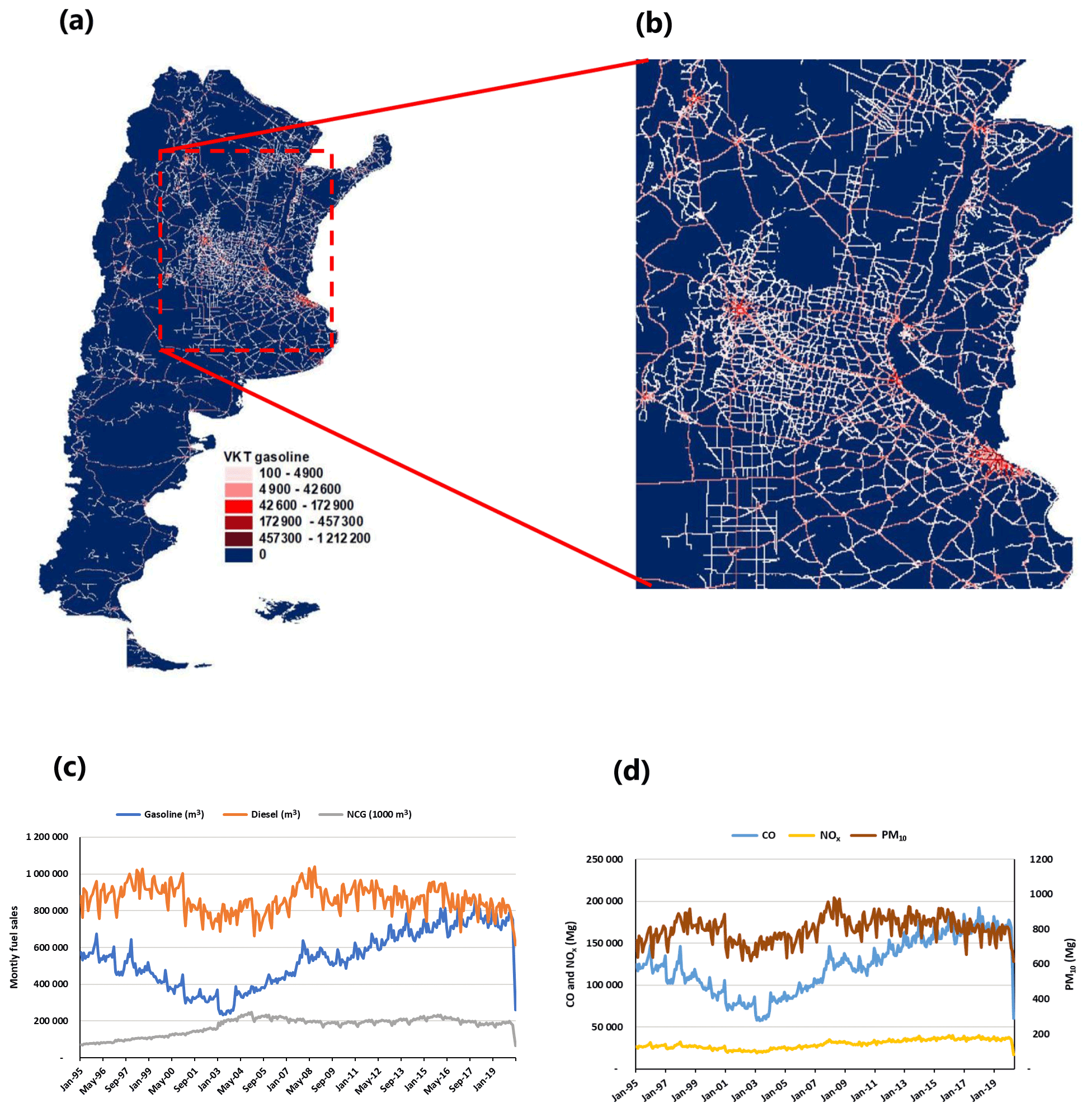
Figure A1Calculated VKT for gasoline vehicles. (b) Calculated VKT for gasoline vehicles in the central area of Argentina. (c) Monthly fuel sales: gasoline (blue line), gas oil (red line), and compressed natural gas (CNG) (black line). (d) Monthly emissions (in megagrams) from road transport between January 1995 and April 2020: CO (blue line) and NOx (black line) on the left axis and PM10 (red line) on the right axis.
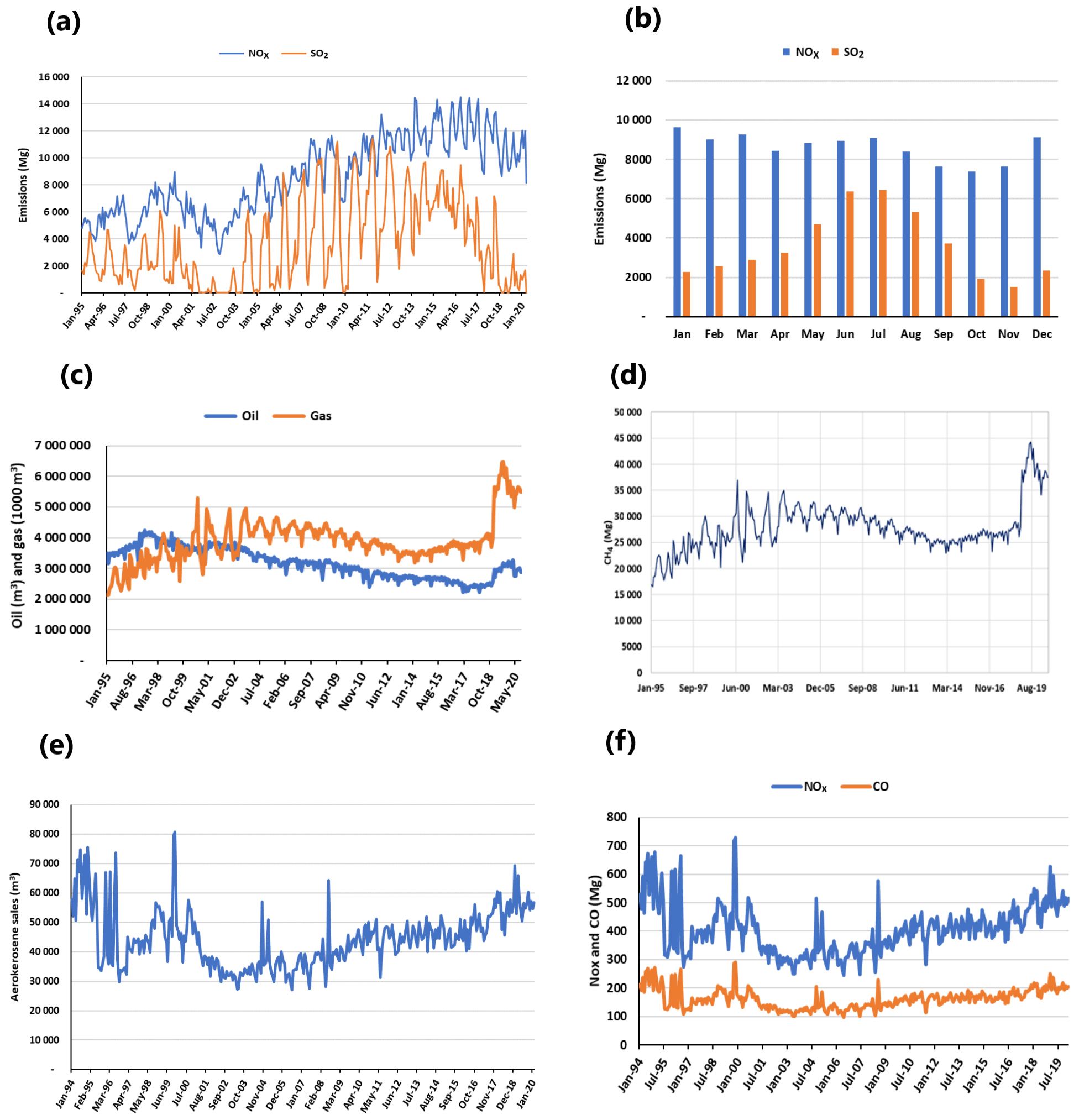
Figure A2(a) Monthly NOx and SO2 emissions (Mg) from thermal power plants. (b) Average seasonal NOx and SO2 emissions 1995–2019 (Mg) from thermal power plants. (c) Monthly oil (m3) and gas production (1000 m3). (d) Monthly methane emissions (Mg) from fuel production. (e) Monthly aerokerosene sales at airports (m3) for domestic and international flights. (f) Monthly CO and NOx emissions from aviation.
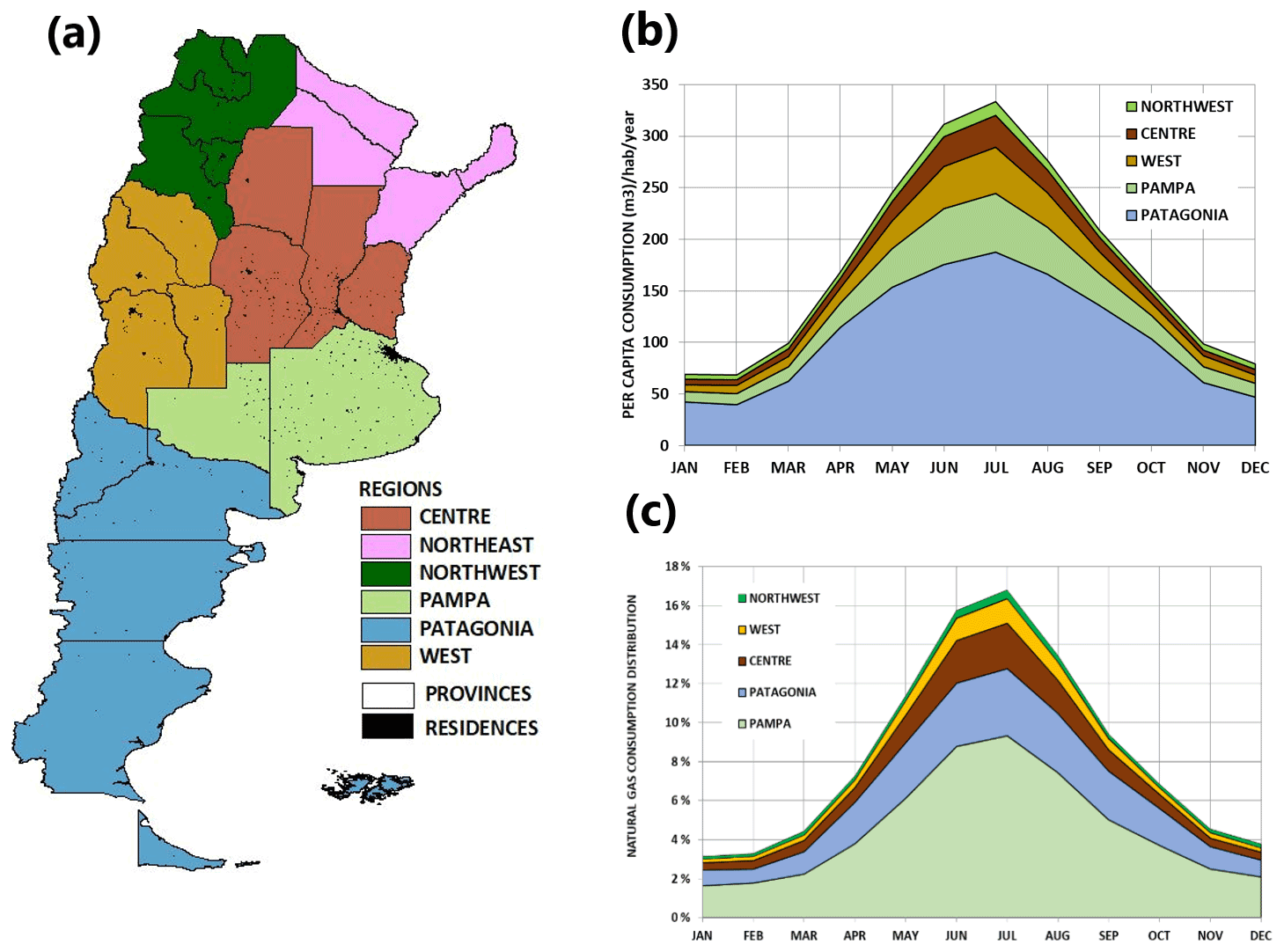
Figure A3(a) Regions and provinces with natural gas consumption at homes. (b) Per capita annual natural gas consumptions. (c) Regional and seasonal distribution of natural gas consumption per region (percent of total annual consumption).

Figure A4(a) Railroad network and navigation ports, (b) seasonal railroad freight (million metric tons per kilometer), and passenger activity (million passengers per kilometer). (c) Monthly railroad activity and fuel consumption (m3) and passenger activity (million passengers per kilometer).
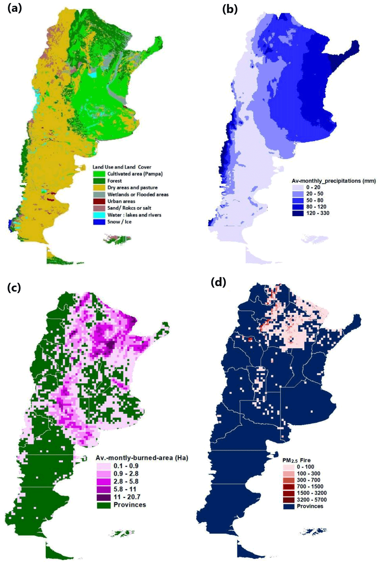
Figure A5(a) Land types for Argentina. (b) Monthly average precipitation (millimeters per cell). (c) Monthly average burned area (hectares per cell). (d) PM2.5 emissions in (kilograms per cell) for September 2017.
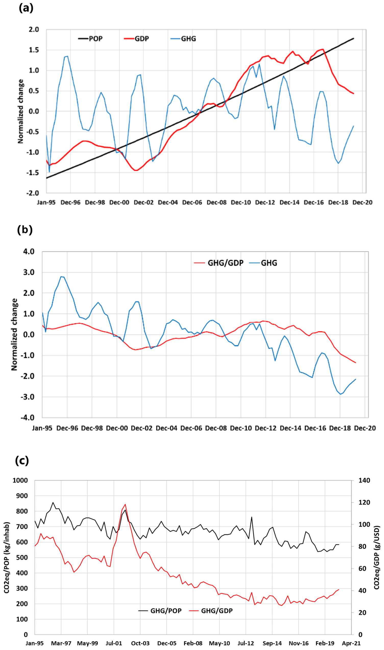
Figure A6Normalized change in (a) population, gross domestic product, and GHGs in terms of CO2eq between 1995 and 2020. (b) Population de-trended GDP and GHG. (c) De-trended GHG cap (GHG emissions per capita (or inhabitants), units: kg/inhabitant) and GHG GDP (GHG emissions per US dollar of gross domestic product, units: g/USD). The normalized function is obtained by subtracting the function mean value and divided by its standard deviation.
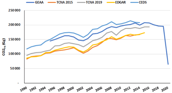
Figure A7Comparison of annual GHG emissions for the energy sector between the different inventories considered in this work (see Table A7.).
Comparison of total annual values for five inventories: GEAA, TCNA2015, TCNA2019, CEDS, and EDGAR
In this section we compare the total annual values for Argentina for the period 1995 through 2015 for several national and international databases. We include the present work GEAA-AEIv3.0M with the Third National Communication of Argentina to the IPCC (TCNA, 2015), which includes annual GHG emissions from 1990 through 2014 and the recent update TCNA 2019 (which spans from 1990 to 2016). Annual total emissions of GHG and air quality pollutants are also compared to the estimations presented in the EDGAR HTAPv5.0 inventory (Crippa et al., 2016, 2020; EDGAR, 2019) and the Community Emissions Data System (CEDS) (Hoesly et al., 2018; McDuffie et al., 2020). We selected those sectors and pollutants that are present in at least three inventories. PM10 and PM25 are only present in EDGAR (Table A10). These contaminants were discussed in the main text.
The file “comp_geaa_ceds_edgar_tcna.xlxs” in the Supplement contains detailed information for each inventory and their comparison. It includes tables and figures, according to Table A6. Tables A7 through Table A10 retrieve some of the main results of the comparisons.
Table A1Argentine inventories developed at the Group for Atmospheric and Environmental Studies (GEAA).
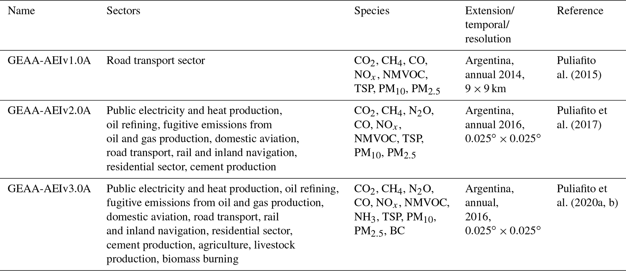
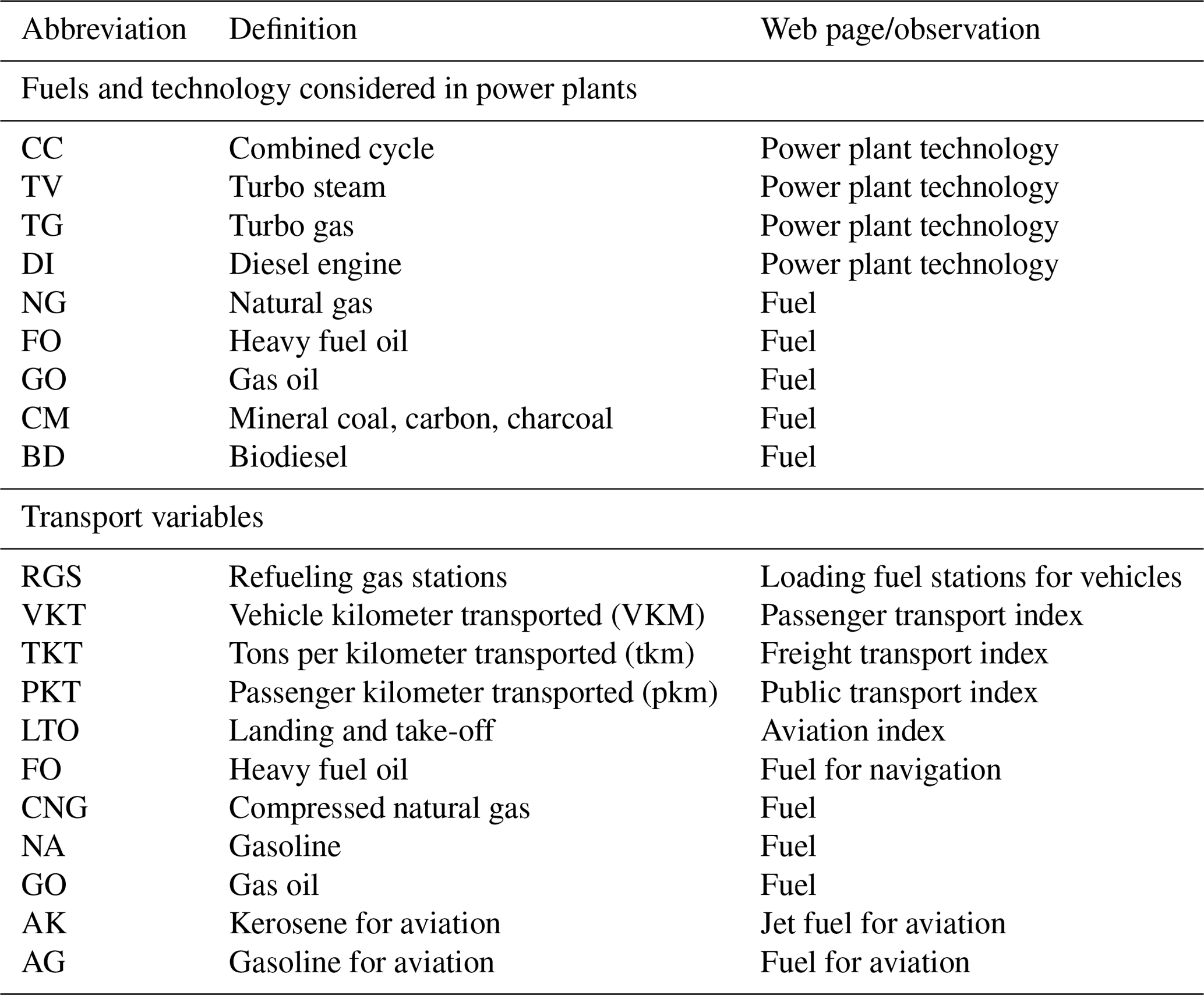
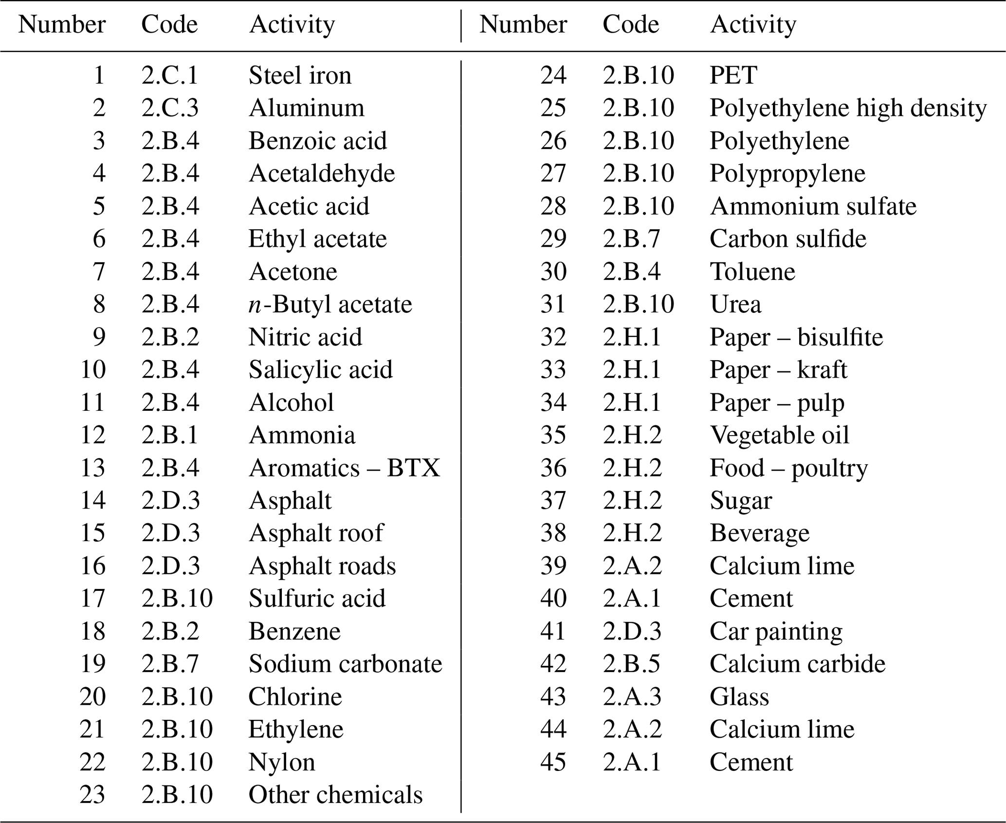
Table A4Summary of pollutants emissions for Argentina during December 2019 and December 1995.
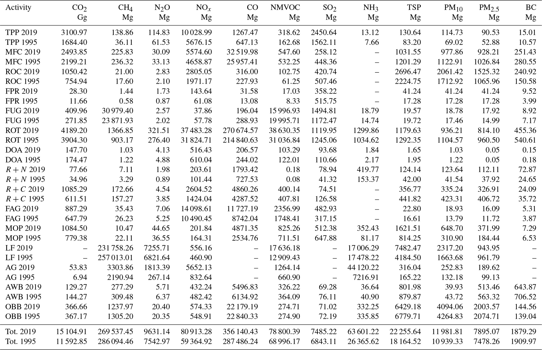
Ref: TPP: power plants; MFC: manufacturing's own fuel consumption; ROC: refinery consumption; FPR: fuel production; FUG: fugitive, venting, and flaring; ROT: road transport; DOA: domestic aviation; R+N: railroad and navigation; R+C: residential and commercial; FAG: fuel use in agriculture; MOP: manufacturing's own process; LF: livestock feeding; AG: agriculture; AWB: agriculture waste burning; OBB: open biomass burning.
Table A5Impact of COVID-19 lockdown on Argentine emissions: summary of monthly emissions for April 2020 and April 2019.
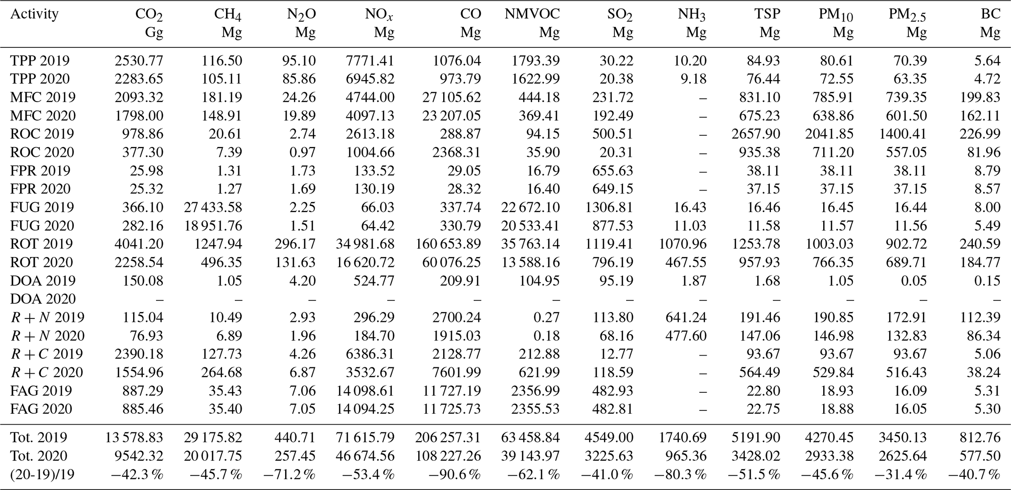
Ref: TPP: power plants; MFC: manufacturing's own fuel consumption; ROC: refinery consumption; FPR: fuel production; FUG: fugitive, venting, and flaring; ROT: road transport; DOA: domestic aviation; R+N: railroad and navigation; R+C: residential and commercial; FAG: fuel use in agriculture.
Table A6Index of comp_geaa_ceds_edgar_tcna.xlxs in the Supplement.
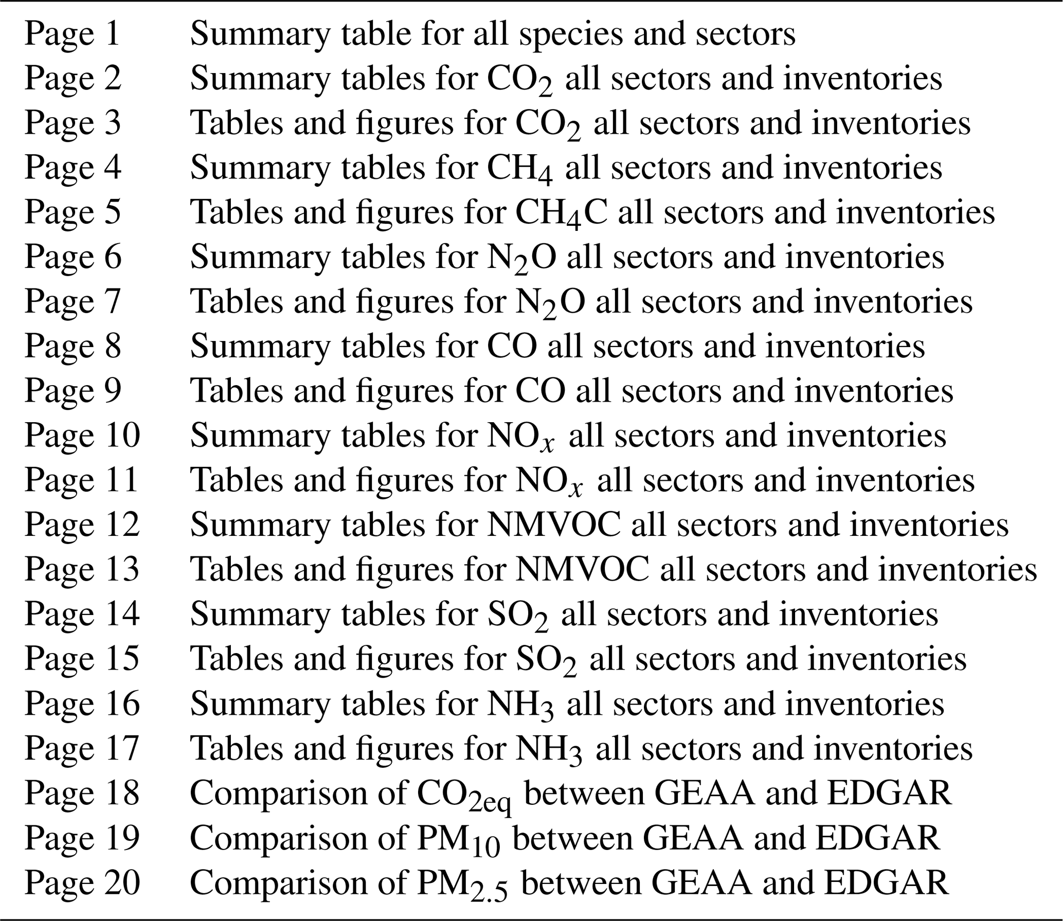
Table A7Comparison of total annual values for five inventories: GEAA, TCNA2015, TCNA2019, CEDS, and EDGAR, 1995–2015.
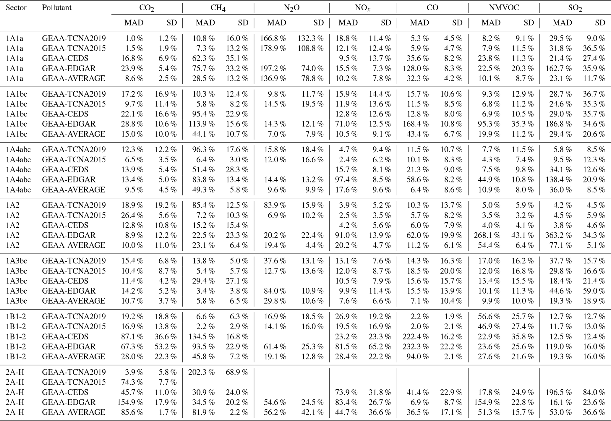
Ref.: MAD: mean absolute differences from two inventories for 1995–2015. SD: standard deviation of two inventories for 1995–2015. GEAA-AVERAGE: differences between GEAA profile and the average of all inventories profile. TCNA2015 (1995–2014); CEDS (1995–2014).
Table A8TCNA 2015 inventory: annual GHG emissions (CO2eq) for Argentina.
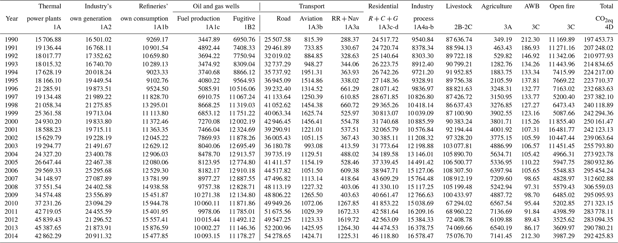
All values are expressed in gigagrams (Gg).
Table A9Comparison of total annual values for GEAA and TCNA 2015 from 1995 through 2014.
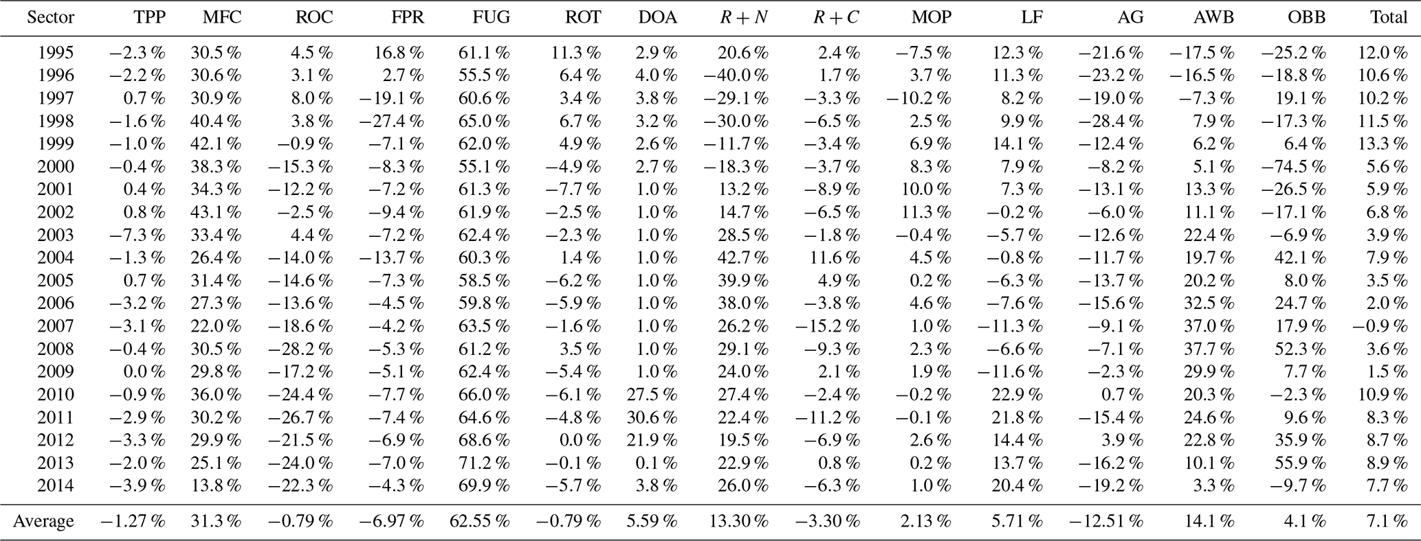
The percentage difference has been computed as . Ref: TPP (1A1): power plants; MFC (1A2): manufacturing's own fuel consumption; ROC (1A1b): refinery consumption; FPR (1A1c): fuel production; FUG (1B2): fugitive, venting, and flaring; ROT (1A3b): road transport; DOA (1A3a): domestic aviation; R+N (1A3c–d): railroad and navigation; R+C (NG) (1A4a–b): residential and commercial; MOP (2B–2C): manufacturing's own process; LF (3A): livestock feeding; AG (3C): agriculture; AWB: agriculture waste burning; OBB (4D): open biomass burning.
Table A10Comparison of total annual values for GEAA and EDGAR from 1995 through 2015 for PM.
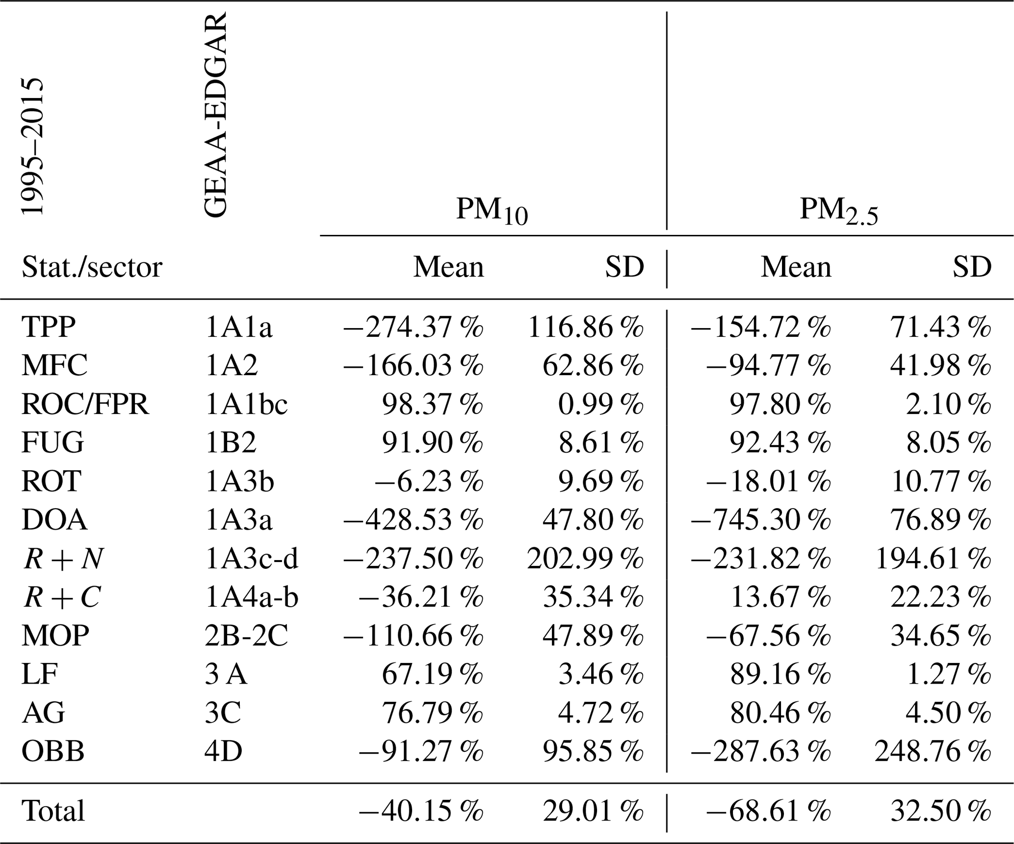
The percentage difference has been computed as . Ref: PP: power plants; MFC: manufacturing's own fuel consumption; ROC: refinery consumption; FPR: fuel production; FUG: fugitive, venting and flaring; ROT: road transport; DOA: domestic aviation; R+N: railroad and navigation; R+C (NG): residential and commercial (natural gas); R+C (OF): residential and commercial (other fuels); FAG: fuel use in agriculture; MOP: manufacturing's own process; LF: livestock feeding; AG: agriculture; AWB: agriculture waste burning; OBB: open biomass burning.
The Supplement related to this article compiles two files: a pdf file with Figs. S1 to S18, which show the monthly and annual variations for the different subsectors analyzed, and a spreadsheet file with the comparison of total annual values for five inventories: GEAA, TCNA2015, TCNA2019, CEDS, and EDGAR. Both are available online. The supplement related to this article is available online at: https://doi.org/10.5194/essd-13-5027-2021-supplement.
SEP and TRBO conceived the conceptualization, methodology, and original writing. SEP and RPF helped perform the formal analysis, supervision and writing. SEP, TRBO, RPF, LLB, RMPF, JU, and AILN contributed to the data organization and investigation. SEP, TRBO, and MFT coordinated the editing. SEP prepared the manuscript with contributions from all co-authors.
The authors declare that they have no conflict of interest.
Publisher's note: Copernicus Publications remains neutral with regard to jurisdictional claims in published maps and institutional affiliations.
This article is part of the special issue “Surface emissions for atmospheric chemistry and air quality modelling”. It is not associated with a conference.
The authors would like to thank Universidad Tecnológica Nacional (UTN) (National Technological University) and Consejo Nacional de Investigaciones Científicas y Técnicas (CONICET) (National Council for Scientific and Technical Investigations) for supporting research activities.
This research has been supported by the Agencia Nacional de Promoción Científica y Tecnológica, Fondo para la Investigación Científica y Tecnológica (FONCYT PICT, grant nos. 2016-1115 and 2016-0714; CONICET PIP, grant no. 112 201101 00673; and UTN PID, grant nos. 1799, 1487, 4920.
This paper was edited by Mauricio Osses and reviewed by two anonymous referees.
Al-Kindi, S. G., Brook, R. D., Biswal, S., and Rajagopalan, S.: Environmental determinants of cardiovascular disease: lessons learned from air pollution, Nat. Rev. Cardiol., 17, 656–672, https://doi.org/10.1038/s41569-020-0371-2, 2020.
Allen, D. T., Torres, V. M., Thomas, J., Sullivan, D. W., Harrison, M., Hendler, A., Herndon, S. C., Kolb, C. E., Fraser, M. P., Hill, A. D., Lamb, B. K., Miskimins, J., Sawyer, R. F., and Seinfeldi, J. H.: Measurements of methane emissions at natural gas production sites in the United States, P. Natl. Acad. Sci. USA, 110, 17768–17773, https://doi.org/10.1073/pnas.1304880110, 2013.
Amann, M., Bertok, I., Borken-Kleefeld, J., Cofala, J., Heyes, C., Höglund-Isaksson, L., Klimont, Z., Nguyen, B., Posch, M., Rafaj, P., Sandler, R., Schöpp, W., Wagner, F., and Winiwarter, W.: Cost-effective control of air quality and greenhouse gases in Europe: Modeling and policy applications, Environ. Modell. Softw., 26, 1489–1501, https://doi.org/10.1016/j.envsoft.2011.07.012, 2011.
Arino, O., Perez, J. R., Kalogirou, V., Defourny, P., and Achard, F.: Global Land Cover Map for 2009 (GlobCover 2009), ESA Living Planet Symp., 27 June–2 July 2010, Bergen, Norway, 31046, 2010.
Arneth, A., Unger, N., Kulmala, M., and Andreae, M. O.: Clean the Air, Heat the Planet?, Science, 326, 672–673, https://doi.org/10.1126/science.1181568, 2009.
Bolaño-Ortiz, T. R., Puliafito, S. E., Berná-Peña, L. L., Pascual-Flores, R. M., Urquiza, J., and Camargo-Caicedo, Y.: Atmospheric Emission Changes and Their Economic Impacts during the COVID-19 Pandemic Lockdown in Argentina, Sustainability, 12, 8661, https://doi.org/10.3390/su12208661, 2020.
Bontemps, S., Defourny, P., Van Bogaert, E., Kalogirou, V., and Perez, J. R.: GLOBCOVER 2009 Products Description and Validation Report, ESA Bull.-Eur. Space, 136, 1–53, 2011.
Cammesa: Electric distribution agency of Argentina – Cammesa, Cammesa database, online, available from: https://portalweb.cammesa.com/pages/Descargas/descargas.aspx, last access: 29 December 2020.
Castesana, P. S., Dawidowski, L. E., Finster, L., Gómez, D. R., and Taboada, M. A.: Ammonia emissions from the agriculture sector in Argentina; 2000–2012, Atmos. Environ., 178, 293–304, https://doi.org/10.1016/j.atmosenv.2018.02.003, 2018.
CIESIN: Socioeconomic Data and Application Center, available at: https://sedac.ciesin.columbia.edu/data/collection/gpw-v3 (last access: 8 October 2021), 2005.
Cimorelli, A. J., Perry, S. G., and Venkatram, A.: AERMOD: Description of model formulation, Report, 44, July 2015, EPA-454/R-03-004, available at: https://nepis.epa.gov/Exe/ZyPURL.cgi?Dockey=P1009OXW.txt (last access: 26 October 2021), 2004.
CNRT: National Transportation Commission (CNRT) – Argentina, Rail Transp. Stat., online, available from: https://www.argentina.gob.ar/transporte/cnrt/estadisticas, last access: 21 December 2020.
Crippa, M., Janssens-Maenhout, G., Dentener, F., Guizzardi, D., Sindelarova, K., Muntean, M., Van Dingenen, R., and Granier, C.: Forty years of improvements in European air quality: regional policy-industry interactions with global impacts, Atmos. Chem. Phys., 16, 3825–3841, https://doi.org/10.5194/acp-16-3825-2016, 2016.
Crippa, M., Solazzo, E., Huang, G., Guizzardi, D., Koffi, E., Muntean, M., Schieberle, C., Friedrich, R., and Janssens-Maenhout, G.: High resolution temporal profiles in the Emissions Database for Global Atmospheric Research, Sci. Data, 7, 121, https://doi.org/10.1038/s41597-020-0462-2, 2020.
de Meij, A., Krol, M., Dentener, F., Vignati, E., Cuvelier, C., and Thunis, P.: The sensitivity of aerosol in Europe to two different emission inventories and temporal distribution of emissions, Atmos. Chem. Phys., 6, 4287–4309, https://doi.org/10.5194/acp-6-4287-2006, 2006.
EDGAR: EDGAR datasets, EDGAR – Arch. datasets, online, available from: https://edgar.jrc.ec.europa.eu/ (last access: 20 January 2021), 2019.
EMEP: EMEP/EEA Air Pollutant Emission Inventory Guidebook – 2013, European Environment Agency, Copenhagen K, Denmark, https://doi.org/10.2800/92722, 2013.
EMEP: EMEP/EEA air pollutant emission inventory guidebook – 2016 – European Environment Agency, EEA Reports, 21, Copenhagen K, Denmark, https://doi.org/10.2800/247535, 2016.
EMEP: EEA Report no. 13/2019, European Environment Agency, Copenhagen K, Denmark, 2019.
EPA: AP-42, Compilation of Air Pollutant Emission Factors, in Pollution Control Handbook for Oil and Gas Engineering, edited by: Cheremisinoff, N. P., U.S. Environmental Protection Agency, Raleigh, NC, USA, 2016.
Etminan, M., Myhre, G., Highwood, E. J., and Shine, K. P.: Radiative forcing of carbon dioxide, methane, and nitrous oxide: A significant revision of the methane radiative forcing, Geophys. Res. Lett., 43, 12614–12623, https://doi.org/10.1002/2016GL071930, 2016.
Ferreyra, M. F. G., Curci, G., and Lanfri, M.: First Implementation of the WRF-CHIMERE-EDGAR Modeling System Over Argentina, IEEE J. Sel. Top. Appl., 9, 5304–5314, https://doi.org/10.1109/JSTARS.2016.2588502, 2016.
Funk, C., Peterson, P., Landsfeld, M., Pedreros, D., Verdin, J., Shukla, S., Husak, G., Rowland, J., Harrison, L., Hoell, A., and Michaelsen, J.: The climate hazards infrared precipitation with stations – a new environmental record for monitoring extremes, Sci. Data, 2, 150066, https://doi.org/10.1038/sdata.2015.66, 2015.
Giglio, L., Loboda, T., Roy, D. P., Quayle, B., and Justice, C. O.: An active-fire based burned area mapping algorithm for the MODIS sensor, Remote Sens. Environ., 113, 408–420, https://doi.org/10.1016/j.rse.2008.10.006, 2009.
Giglio, L., Randerson, J. T., and van der Werf, G. R.: Analysis of daily, monthly, and annual burned area using the fourth-generation global fire emissions database (GFED4), J. Geophys. Res.-Biogeo., 118, 317–328, https://doi.org/10.1002/jgrg.20042, 2013.
Gilliland, A. B., Dennis, R. L., Roselle, S. J., and Pierce, T. E.: Seasonal NH3 emission estimates for the eastern United States based on ammonium wet concentrations and an inverse modeling method, J. Geophys. Res.-Atmos., 108, ACH 20-1–ACH 20-12, https://doi.org/10.1029/2002jd003063, 2003.
González, C. M., Ynoue, R. Y., Vara-Vela, A., Rojas, N. Y., and Aristizábal, B. H.: High-resolution air quality modeling in a medium-sized city in the tropical Andes: Assessment of local and global emissions in understanding ozone and PM10 dynamics, Atmos. Pollut. Res., 9, 934–948, https://doi.org/10.1016/j.apr.2018.03.003, 2018.
Grell, G. A., Peckham, S. E., Schmitz, R., McKeen, S. A., Frost, G., Skamarock, W. C., and Eder, B.: Fully coupled “online” chemistry within the WRF model, Atmos. Environ., 39, 6957–6975, https://doi.org/10.1016/J.ATMOSENV.2005.04.027, 2005.
Haines, A., Amann, M., Borgford-Parnell, N., Leonard, S., Kuylenstierna, J., and Shindell, D.: Short-lived climate pollutant mitigation and the Sustainable Development Goals, Nat. Clim. Change, 7, 863–869, https://doi.org/10.1038/s41558-017-0012-x, 2017.
Hallett, J.: Climate change 2001: The scientific basis, edited by: Houghton, J. T., Ding, Y., Griggs, D. J., Noguer, N., van der Linden, P. J., Xiaosu, D., Maskell, K., and Johnson, C. A., Contribution of Working Group I to the Third Assessment Report of the Intergovernmental Panel on Climate Change, Cambridge University Press, Cambridge, 2001, 881 pp., Q. J. Roy. Meteor. Soc., 128, 1038–1039, https://doi.org/10.1002/qj.200212858119, 2002.
Hoesly, R. M., Smith, S. J., Feng, L., Klimont, Z., Janssens-Maenhout, G., Pitkanen, T., Seibert, J. J., Vu, L., Andres, R. J., Bolt, R. M., Bond, T. C., Dawidowski, L., Kholod, N., Kurokawa, J.-I., Li, M., Liu, L., Lu, Z., Moura, M. C. P., O'Rourke, P. R., and Zhang, Q.: Historical (1750–2014) anthropogenic emissions of reactive gases and aerosols from the Community Emissions Data System (CEDS), Geosci. Model Dev., 11, 369–408, https://doi.org/10.5194/gmd-11-369-2018, 2018.
Huneeus, N., Denier van der Gon, H., Castesana, P., Menares, C., Granier, C., Granier, L., Alonso, M., de Fatima Andrade, M., Dawidowski, L., Gallardo, L., Gomez, D., Klimont, Z., Janssens-Maenhout, G., Osses, M., Puliafito, S. E., Rojas, N., Sánchez-Ccoyllo, O., Tolvett, S., and Ynoue, R. Y.: Evaluation of anthropogenic air pollutant emission inventories for South America at national and city scale, Atmos. Environ., 235, 117606, https://doi.org/10.1016/j.atmosenv.2020.117606, 2020.
IGN: National Geographic Institute of the Argentine Republic, Polit. Div. Surf. Popul. ARGENTINA, online, available from: https://www.ign.gob.ar/NuestrasActividades/Geografia/DatosArgentina/DivisionPolitica, last access: 26 December 2020.
INDEC: Population projections by province in Argentina, Popul. Proj. by Prov. Argentina, online, available from: https://www.indec.gob.ar/indec/web/Nivel4-Tema-2-24-85, last access: 15 December 2020.
IPCC: Climate Change 2014: Synthesis Report, Contribution of Working Groups I, II and III to the Fifth Assessment Report of the Intergovernmental Panel on Climate Change, edited by: Core Writing Team, Pachauri, R. K., and Meyer, L. A., Geneva, Switzerland, 2014.
Isaksen, I. S. A., Granier, C., Myhre, G., Berntsen, T. K., Dalsøren, S. B., Gauss, M., Klimont, Z., Benestad, R., Bousquet, P., Collins, W., Cox, T., Eyring, V., Fowler, D., Fuzzi, S., Jöckel, P., Laj, P., Lohmann, U., Maione, M., Monks, P., Prevot, A. S. H., Raes, F., Richter, A., Rognerud, B., Schulz, M., Shindell, D., Stevenson, D. S., Storelvmo, T., Wang, W.-C., van Weele, M., Wild, M., and Wuebbles, D.: Atmospheric composition change: Climate–Chemistry interactions, Atmos. Environ., 43, 5138–5192, https://doi.org/10.1016/j.atmosenv.2009.08.003, 2009.
Jacob, D. J. and Winner, D. A.: Effect of climate change on air quality, Atmos. Environ., 43, 51–63, https://doi.org/10.1016/j.atmosenv.2008.09.051, 2009.
Janssens-Maenhout, G., Crippa, M., Guizzardi, D., Muntean, M., Schaaf, E., Dentener, F., Bergamaschi, P., Pagliari, V., Olivier, J. G. J., Peters, J. A. H. W., van Aardenne, J. A., Monni, S., Doering, U., Petrescu, A. M. R., Solazzo, E., and Oreggioni, G. D.: EDGAR v4.3.2 Global Atlas of the three major greenhouse gas emissions for the period 1970–2012, Earth Syst. Sci. Data, 11, 959–1002, https://doi.org/10.5194/essd-11-959-2019, 2019.
Klimont, Z., Kupiainen, K., Heyes, C., Purohit, P., Cofala, J., Rafaj, P., Borken-Kleefeld, J., and Schöpp, W.: Global anthropogenic emissions of particulate matter including black carbon, Atmos. Chem. Phys., 17, 8681–8723, https://doi.org/10.5194/acp-17-8681-2017, 2017.
Kumar, A., Dixit, S., Varadarajan, C., Vijayan, A., and Masuraha, A.: Evaluation of the AERMOD dispersion model as a function of atmospheric stability for an urban area, Environ. Prog., 25, 141–151, https://doi.org/10.1002/ep.10129, 2006.
Lee, H. D., Yoo, J. W., Kang, M. K., Kang, J. S., Jung, J. H., and Oh, K. J.: Evaluation of concentrations and source contribution of PM10 and SO2 emitted from industrial complexes in Ulsan, Korea: Interfacing of the WRF-CALPUFF modeling tools, Atmos. Pollut. Res., 5, 664–676, https://doi.org/10.5094/APR.2014.076, 2014.
Li, M., Liu, H., Geng, G., Hong, C., Liu, F., Song, Y., Tong, D., Zheng, B., Cui, H., Man, H., Zhang, Q., and He, K.: Anthropogenic emission inventories in China: A review, Natl. Sci. Rev., 4, 834–866, https://doi.org/10.1093/nsr/nwx150, 2017.
McDuffie, E. E., Smith, S. J., O'Rourke, P., Tibrewal, K., Venkataraman, C., Marais, E. A., Zheng, B., Crippa, M., Brauer, M., and Martin, R. V.: A global anthropogenic emission inventory of atmospheric pollutants from sector- and fuel-specific sources (1970–2017): an application of the Community Emissions Data System (CEDS), Earth Syst. Sci. Data, 12, 3413–3442, https://doi.org/10.5194/essd-12-3413-2020, 2020.
Minem: Ministry of Energy – Argentina, Open database from Argentine Minist. Energy, online, available from: http://datos.minem.gob.ar/dataset?groups=comercializacion-de-los-hidrocarburos, last access: 27 December 2020.
Myhre, G., Berglen, T. F., Johnsrud, M., Hoyle, C. R., Berntsen, T. K., Christopher, S. A., Fahey, D. W., Isaksen, I. S. A., Jones, T. A., Kahn, R. A., Loeb, N., Quinn, P., Remer, L., Schwarz, J. P., and Yttri, K. E.: Modelled radiative forcing of the direct aerosol effect with multi-observation evaluation, Atmos. Chem. Phys., 9, 1365–1392, https://doi.org/10.5194/acp-9-1365-2009, 2009.
Myhre, G., Shindell, D., Bréon, F.-M., Collins, W., Fuglestvedt, J., Huang, J., Koch, D., Lamarque, J.-F., Lee, D., Mendoza, B., Nakajima, T., Robock, A., Stephens, G., Takemura, T., Zhan, H., and Zhang, H.: Anthropogenic and Natural Radiative Forcing: Supplementary Material, Clim. Chang. 2013 Phys. Sci. Basis. Contrib. Work. Gr. I to Fifth Assess. Rep. Intergov. Panel, Cambridge University Press, Cambridge, UK, 659–740, https://doi.org/10.1017/CBO9781107415324.018, 2013.
Nakicenovic, N., Alcamo, J., Davis, G., de Vries, B., Fenhann, J., Gaffin, S., Gregory, K., Grübler, A., Jung, T. Y., Kram, T., La Rovere, E. L., Michaelis, L., Mori, S., Morita, T., Pepper, W., Pitcher, H., Price, L., Raihi, K., Roehrl, A., Rogner, H.-H., Sankovski, A., Schlesinger, M., Shukla, P., Smith, S., Swart, R., van Rooijen, S., and Victor, D. Z.: IPCC Special Report on Emissions Scenarios, Cambridge University Press, Cambridge, UK, 2000.
Puliafito, S. E., Allende, D., Pinto, S., and Castesana, P.: High resolution inventory of GHG emissions of the road transport sector in Argentina, Atmos. Environ., 101, 303–311, https://doi.org/10.1016/j.atmosenv.2014.11.040, 2015.
Puliafito, S. E., Allende, D. G., Castesana, P. S., and Ruggeri, M. F.: High-resolution atmospheric emission inventory of the argentine energy sector. Comparison with edgar global emission database, Heliyon, 3, e00489, https://doi.org/10.1016/j.heliyon.2017.e00489, 2017.
Puliafito, S. E., Bolaño-Ortiz, T., Berná, L., and Pascual Flores, R.: High resolution inventory of atmospheric emissions from livestock production, agriculture, and biomass burning sectors of Argentina, Atmos. Environ., 223, 117248, https://doi.org/10.1016/j.atmosenv.2019.117248, 2020a.
Puliafito, S. E., Bolaño-Ortiz, T. R., Berná Peña, L. L., and Pascual-Flores, R. M.: Dataset supporting the estimation and analysis of high spatial resolution inventories of atmospheric emissions from several sectors in Argentina, Data in Brief, 29, 105281, https://doi.org/10.1016/j.dib.2020.105281, 2020b.
Puliafito, S. E., Bolaño-Ortiz, T. R., Fernandez, R. P., Berná, L. L., Pascual-Flores, R. M., Urquiza, J., López-Noreña, A. I., and Tames, M. F.: Data for: High resolution seasonal and decadal inventory of anthropic gas-phase and particle emissions for Argentina, Mendeley Data [data set], https://doi.org/10.17632/d6xrhpmzdp.2, 2021.
Ramanathan, V., Crutzen, P. J., Kiehl, J. T., and Rosenfeld, D.: Atmosphere: Aerosols, climate, and the hydrological cycle, Science, 294, 2119–2124, https://doi.org/10.1126/science.1064034, 2001.
Ravishankara, A. R., Daniel, J. S., and Portmann, R. W.: Nitrous Oxide (N2O): The Dominant Ozone-Depleting Substance Emitted in the 21st Century, Science, 326, 123–125, https://doi.org/10.1126/science.1176985, 2009.
Rivera, J. A., Marianetti, G., and Hinrichs, S.: Validation of CHIRPS precipitation dataset along the Central Andes of Argentina, Atmos. Res., 213, 437–449, https://doi.org/10.1016/J.ATMOSRES.2018.06.023, 2018.
Rodriguez, E., Morris, C. S., Belz, J. E., Chapin, E. C., Martin, J. M., Daffer, W., and Hensley, S.: An assessment of the SRTM topographic products, NASA Jet Propulsion Laboratory, Pasadema, CA, USA, 2005.
Rood, A. S.: Performance evaluation of AERMOD, CALPUFF, and legacy air dispersion models using the Winter Validation Tracer Study dataset, Atmos. Environ., 89, 707–720, https://doi.org/10.1016/j.atmosenv.2014.02.054, 2014.
Roscioli, J. R., Yacovitch, T. I., Floerchinger, C., Mitchell, A. L., Tkacik, D. S., Subramanian, R., Martinez, D. M., Vaughn, T. L., Williams, L., Zimmerle, D., Robinson, A. L., Herndon, S. C., and Marchese, A. J.: Measurements of methane emissions from natural gas gathering facilities and processing plants: measurement methods, Atmos. Meas. Tech., 8, 2017–2035, https://doi.org/10.5194/amt-8-2017-2015, 2015.
Rystad: Rystad energy, Will vast potential Argentina's Vaca Muerta shale Play ever be unlocked?, online, available from: https://www.rystadenergy.com/newsevents/events/rystad-energy-webinars/webinar/915-shale-webinar-will-the-vast-potential-of-argentina-s-vaca-muerta-shale-play-ever-be-unlocked- (last access: 24 November 2020), 2018.
Sato, A., Vitullo, M., and Gschwantner, T.: Chapyer 8 Settlements – 2019 Refinement to the 2006 IPCC Guidelines for National Greenhouse Gas Inventories, Cambridge University Press, Cambridge, United Kingdom and New York, NY, USA, 2019.
Scire, J. S., Strimaitis, D. G., and Yamartino, R. J.: A User's Guide for the CALPUFF Dispersion Model, Earth Tech. Inc, Concord, MA, USA, 2000.
Shindell, D. T.: The social cost of atmospheric release, Clim. Change, 130, 313–326, https://doi.org/10.1007/s10584-015-1343-0, 2015.
Shindell, D. T., Walter, B. P., and Faluvegi, G.: Impacts of climate change on methane emissions from wetlands, Geophys. Res. Lett., 31, L21202, https://doi.org/10.1029/2004GL021009, 2004.
Solomon, S., Plattner, G.-K., Knutti, R., and Friedlingstein, P.: Irreversible climate change due to carbon dioxide emissions, P. Natl. Acad. Sci. USA, 106, 1704 LP – 1709, https://doi.org/10.1073/pnas.0812721106, 2009.
Solomon, S., Alcamo, J., and Ravishankara, A. R.: Unfinished business after five decades of ozone-layer science and policy, Nat. Commun., 11, 4272, https://doi.org/10.1038/s41467-020-18052-0, 2020.
SSPYVN: National Port Authority (SSPYVN) – Argentina, Load. Stat. data, online, available from: https://www.argentina.gob.ar/puertos-vias-navegables-y-marina-mercante/estadisticas-de-carga, last access: 29 December 2020.
Stohl, A., Aamaas, B., Amann, M., Baker, L. H., Bellouin, N., Berntsen, T. K., Boucher, O., Cherian, R., Collins, W., Daskalakis, N., Dusinska, M., Eckhardt, S., Fuglestvedt, J. S., Harju, M., Heyes, C., Hodnebrog, Ø., Hao, J., Im, U., Kanakidou, M., Klimont, Z., Kupiainen, K., Law, K. S., Lund, M. T., Maas, R., MacIntosh, C. R., Myhre, G., Myriokefalitakis, S., Olivié, D., Quaas, J., Quennehen, B., Raut, J.-C., Rumbold, S. T., Samset, B. H., Schulz, M., Seland, Ø., Shine, K. P., Skeie, R. B., Wang, S., Yttri, K. E., and Zhu, T.: Evaluating the climate and air quality impacts of short-lived pollutants, Atmos. Chem. Phys., 15, 10529–10566, https://doi.org/10.5194/acp-15-10529-2015, 2015.
Tartakovsky, D., Broday, D. M., and Stern, E.: Evaluation of AERMOD and CALPUFF for predicting ambient concentrations of total suspended particulate matter (TSP) emissions from a quarry in complex terrain, Environ. Pollut., 179, 138–145, https://doi.org/10.1016/j.envpol.2013.04.023, 2013.
TCNA: Third National Communication of Argentina to the IPCC, City of Buenos Aires., online, available from: https://unfccc.int/documents/67499 (last access: 20 February 2021), 2015.
TCNA: Third Bienal Upadate of National Communication of Argentina to the IPCC, City of Buenos Aires., online, available from: https://inventariogei.ambiente.gob.ar/resultados (last access: 20 February 2021), 2019.
Thompson, R. L., Lassaletta, L., Patra, P. K., Wilson, C., Wells, K. C., Gressent, A., Koffi, E. N., Chipperfield, M. P., Winiwarter, W., Davidson, E. A., Tian, H., and Canadell, J. G.: Acceleration of global N2O emissions seen from two decades of atmospheric inversion, Nat. Clim. Change, 9, 993–998, https://doi.org/10.1038/s41558-019-0613-7, 2019.
Trossero, M., Drigo, R., Anschau, A., Carballo, S., and Flores Marco, N.: Análisis del balance de energía derivada de biomasa en Argentina, WISDOM, ARGENTINA, Wood fuel Integrated Supply/Demand Overview Mapping, Instituto de Tecnología Agropecuaria, available at: https://www.fao.org/3/i0900s/i0900s00.pdf (last access: 26 December 2020), 2009.
UNEP: United Nations Environment Programme, Nairobi, Kenia, 2013.
UNEP-WMO: Integrated Assessment of Black Carbon and Tropospheric Ozone, United Nations Environ. Program (UNEP), Nairobi, Kenya., UNEP/GC.26/INF/20, 2011.
Volante, J. N., Collado, A., Ferreyra, E. B., López, C., Navarro, M., Pezzola, A., and Puentes, M. I.: Informe Técnico Unificado PNECO 1643, Monitoreo de la Cobertura y el Uso del Suelo a partir de sensores remotos. Programa Nacional de Ecorregiones, INTA, Buenos Aires, Argentina. Land use Map of Argentina, available at: http://www.geointa.inta.gob.ar/2013/05/19/cobertura-del-suelo-de-la-republica-argentina/ (last access: 27 October 2021), 2009.
West, J. J., Fiore, A. M., Horowitz, L. W., and Mauzerall, D. L.: Global health benefits of mitigating ozone pollution with methane emission controls, P. Natl. Acad. Sci. USA, 103, 3988–3993, https://doi.org/10.1073/pnas.0600201103, 2006.
Ying, Z., Tie, X., and Li, G.: Sensitivity of ozone concentrations to diurnal variations of surface emissions in Mexico City: A WRF/Chem modeling study, Atmos. Environ., 43, 851–859, https://doi.org/10.1016/j.atmosenv.2008.10.044, 2009.
Zavala-Araiza, D., Sullivan, D. W., and Allen, D. T.: Atmospheric hydrocarbon emissions and concentrations in the barnett shale natural gas production region, Environ. Sci. Technol., 48, 5314–5321, https://doi.org/10.1021/es405770h, 2014.
- Abstract
- Introduction
- Material and methods
- Results
- Inter-comparison of GEAA-AEIv3.0M with other emissions inventories for Argentina
- Data availability
- Conclusions
- Appendix A
- Author contributions
- Competing interests
- Disclaimer
- Special issue statement
- Acknowledgements
- Financial support
- Review statement
- References
- Supplement