the Creative Commons Attribution 4.0 License.
the Creative Commons Attribution 4.0 License.
 | 28 Oct 2021
Laboratory data on wave propagation through vegetation with following and opposing currents
Simei Lian
Huaiyu Wei
Yulong Li
Marcel Stive
Tomohiro Suzuki
Coastal vegetation has been increasingly recognized as an effective buffer against wind waves. Recent laboratory studies have considered realistic vegetation traits and hydrodynamic conditions, which advanced our understanding of the wave dissipation process in vegetation (WDV) in field conditions. In intertidal environments, waves commonly propagate into vegetation fields with underlying tidal currents, which may alter the WDV process. A number of experiments addressed WDV with following currents, but relatively few experiments have been conducted to assess WDV with opposing currents. Additionally, while the vegetation drag coefficient is a key factor influencing WDV, it is rarely reported for combined wave–current flows. Relevant WDV and drag coefficient data are not openly available for theory or model development. This paper reports a unique dataset of two flume experiments. Both experiments use stiff rods to mimic mangrove canopies. The first experiment assessed WDV and drag coefficients with and without following currents, whereas the second experiment included complementary tests with opposing currents. These two experiments included 668 tests covering various settings of water depth, wave height, wave period, current velocity and vegetation density. A variety of data, including wave height, drag coefficient, in-canopy velocity and acting force on mimic vegetation stem, are recorded. This dataset is expected to assist future theoretical advancement on WDV, which may ultimately lead to a more accurate prediction of wave dissipation capacity of natural coastal wetlands. The dataset is available from figshare with clear instructions for reuse (https://doi.org/10.6084/m9.figshare.13026530.v2, Hu et al., 2020). The current dataset will expand with additional WDV data from ongoing and planned observation in natural mangrove wetlands.
- Article
(6593 KB) - Full-text XML
- BibTeX
- EndNote


Coastal wetlands, such as mangroves, salt marshes and seagrasses, are increasingly recognized as effective buffers against wind waves. They can efficiently reduce incident wave height, even in storm conditions (Möller et al., 2014; van Loon-Steensma et al., 2014, 2016; Vuik et al., 2016). Therefore, ecosystem-based coastal defense systems have been proposed as a cost-effective and ecologically sound alternative to conventional coastal engineering (Temmerman et al., 2013; Arkema et al., 2017; Leonardi et al., 2018). These new coastal defense systems have been brought into practice in the Netherlands and the US as “living shorelines” (Borsje et al., 2017; Currin, 2019), which may be adapted in many other areas around the globe.
Since the first theoretical work by Dalrymple et al. (1984), wave dissipation by vegetation (WDV) has been extensively studied through field surveys (e.g., Jadhav et al., 2013; Vuik et al., 2016; Garzon et al., 2019), laboratory experiments (e.g., Lara et al., 2016; Yao et al., 2018; He et al., 2019; Tinoco et al., 2020), and theoretical and numerical models (e.g., Méndez and Losada, 2004; Losada et al., 2016; Hu et al., 2019; Suzuki et al., 2019). Among others, flume and wave basin experiments examining WDV in controlled and repeatable conditions have revealed that WDV is affected by both vegetation canopy traits and hydrodynamic conditions, e.g., water depth, wave period and wave height. The obtained datasets show that increases with vegetation density, stem stiffness and incident wave height (Augustin et al., 2009; Anderson and Smith, 2014), while it decreases with the submergence ratio (the ratio between water depth h and canopy height hv, Stratigaki et al., 2011; Maza et al., 2015). Recent experiments introduced more realistic vegetation morphology (He et al., 2019; Maza et al., 2019) and even real vegetation (Ozeren et al., 2014; Lara et al., 2016) to fully reveal the WDV process in natural coastal wetlands.
In intertidal environments, tidal currents generally flow into the vegetation wetlands in the same direction as incident waves during flooding tide and revise during ebb tide. Using waves as a reference, the underlying currents that flow in the same direction as waves are defined as following currents, whereas the underlying currents that flow in the oppose direction to waves are defined as opposing currents. A number of experiments have tested the impact of coexisting following currents on WDV (Li and Yan, 2007; Paul et al., 2012; Hu et al., 2014). They have shown that following currents can both promote and suppress WDV depending on the ratio between imposed current velocity and amplitude of horizontal orbital velocity (). As contrast, there are fewer experiments that include opposing currents (Ota et al., 2005; Maza et al., 2015). Maza et al. (2015) conducted a unique experiment in a wave basin to investigate the effect of both following and opposing currents on the WDV of submerged canopies. However, emergent conditions were not included in Maza et al. (2015), which is very like to occur in, e.g., tall mangrove forests. Additionally, although recent experiments have improved our understanding of WDV in combined wave–current flows (Losada et al., 2016; Lei and Nepf, 2019), to our knowledge, these experimental datasets are not openly accessible to the research community to foster further advances.
To understand and assess WDV, the knowledge of vegetation drag coefficient (CD) and its variation in different flow conditions is critical. CD is an empirical parameter that links known velocity (u, either from measurements or modeling) to the drag force exerted by vegetation stems (Fd ∼ CD⋅u2, Morison et al., 1950), which is directly related to WDV. Thus, the determination of CD is important to accurate WDV assessment. Its variation with characteristic hydrodynamic parameters, i.e., Reynolds number Re) and Keulegan–Carpenter number KC), has been extensively investigated (Nepf, 2011). CD is commonly derived by calibration method, i.e., calibrating the CD value to ensure the modeled WDV fits with the observation (e.g., Méndez and Losada, 2004; Li and Yan, 2007; Koftis et al., 2013). A more recent direct measurement method has been proposed to derive CD via analyzing synchronized Fd and u on the vegetation stems (Hu et al., 2014; Chen et al., 2018). Such a method does not rely on WDV models but is based on the original Morison equation, Morison et al., 1950). Thus, it can avoid potential errors introduced by WDV models and be readily applied in combined current–wave conditions. However, CD and Fd in combined current–wave flow conditions have been much less reported, especially when waves coexist with opposing currents. To our knowledge, there is no such dataset available that enables further analysis.
This paper presents a combined dataset composed of two flume experiments on WDV with underlying currents in both emergent and submerged conditions (Hu et al., 2020). These two experiments were conducted in 2014 and 2019, respectively (hereafter referred to as E14 and E19). Both experiments applied stiff wooden cylinders to mimic wooden mangrove canopies. In total, E14 conducted 314 tests, and E19 conducted 354 cases with different scenarios of incident waves, imposed current, vegetation density and submergence ratio (Table B1). E14 has systematically compared the variations of WDV and CD with or without coexisting following currents (Hu et al., 2014). As complementary to the E14, E19 further conducted tests with opposing currents. To our knowledge, it is the first freely assessable dataset that includes a wide range of current–wave combinations. Besides wave height variations, this new dataset contains detailed time series data of FD and u in all the tests and velocity profiles in a few selected tests. These data are essential in assessing CD and WDV. It is expected to serve future laboratory, theoretical and numerical studies on WDV, which may eventually lead to a more accurate prediction of wave dissipation efficiency of natural coastal wetlands. The potential usage of this dataset and future avenues to advance our understanding are discussed.
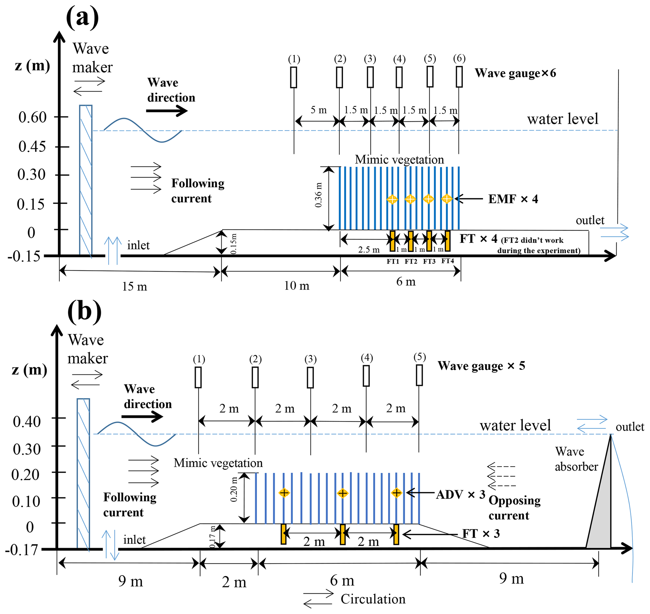
Figure 1Diagrams of the flume experiments. (a) Flume setup of E14, in which waves were imposed either without current or with following currents. EMF refers to electromagnetic flow meters for velocity measurements. FT is the force transducer that can measure the total force on a mimic stem. (b) Flume setup of E19, in which additional tests of waves with opposing currents were included.
2.1 Flume setup of E14
E14 was conducted in the Fluid Mechanics Laboratory at the Delft University of Technology in 2014 (Hu et al., 2014). The used wave flume was 40 m long and 0.8 m wide (Fig. 1a). Currents were imposed in the same direction of the wave propagation, i.e., following currents. We used stiff wooden rods that were fixed vertically on a false bottom as vegetation mimics. The length of the mimic mangrove canopy was 6 m, which was made of wooden rods. The height (hv) and diameter (bv) of the rods was 0.36 and 0.01 m, respectively. Tested water depth (h = 0.25 and 0.5 m) is chosen to mimic emergent and submerged conditions (Table B1). To avoid complex forcing on vegetation stems, in emergent conditions, the wave crests were always lower than the top of the canopy, whereas in submerged conditions, the wave troughs were always higher than the top of the canopy. In the emergent and submerged conditions, the submergence ratios () were 1 and 1.39, respectively. The tested stem densities were Nv = 62, 139 and 556 stems m−2, denoted as VD1, VD2 and VD3, respectively (Table B1). The mimics were placed following a regular stagger pattern (Fig. B1). To measure the wave height attenuation caused by the friction of flume bed and sidewalls, control tests with no mimic stems (VD0) were also tested.
In E14, wave height variation was measured by six capacitance-type wave gauges (WG1–WG6) installed in the flume (Fig. 1a). The capacitance-type wave gauges were made by Deltares, and their accuracy was ± 0.5 % (Delft Hydraulics, year unknown). Force transducers (FT1–4) were installed to measure the acting force F on four individual vegetation mimics along with the canopy (Figs. 1a and A1). To minimize disturbance to the flow, all the FTs were installed underneath the false bottom. FT1 and FT3 were developed by Deltares, the Netherlands, whereas FT2 and FT4 were force transducers made by UTILCELL (model 300). The output of FTs is in voltage, and it can be converted to acting force in both positive and negative directions by linear regressions. The calibration was done similarly to Stewart (2004). The output value does not change with the positions of the forcing on the attached vegetation mimics; i.e., the same force gives the same value no matter where the force is acting on the mimics. Force data were sampled at 1000 Hz to capture force variation within a wave period. The accuracy of the FTs was estimated to be ± 1 %, and more details on the FTs can be found in Bouma et al. (2005). FT2 (the second one in the wave direction) failed during the experiment, and the resulting data were excluded for analysis.
Velocity (u) was measured at half water depth by EMFs (electromagnetic flow meters) made by Deltares (accuracy ± 1 %, Delft Hydraulics, 1990). Four EMFs were installed at the same cross sections as the force transducers to obtain in-phase horizontal velocity (Fig. 1a) and subsequently used to derive vegetation drag coefficient (CD). The deriving method is detailed in Appendix C. The velocity measurement was to obtain representative in-canopy velocities. Thus, in submerged canopies, it was perhaps more suitable to measure velocity at half of the canopy height than at half water depth. However, given the relatively shallow water depths tested in both E14 and E19, velocities obtained at both positions were similar, as shown in the vertical velocity profiles (see Fig. 4). These vertical velocity profiles were measured in a few selected cases (see Appendix B). It was done by moving the measuring probes vertically in repeat experiment runs. The velocity profiles were measured in the vegetation canopies far away from both ends of the flumes to avoid the potential local influence of the inlets and outlets.
2.2 Flume setup of E19
E19 was conducted in the Coastal Dynamics Laboratory at Sun Yat-sen University. As a complement to E14, E19 included cases of pure wave, wave with following currents and additional cases of wave with opposing currents. It was conducted in a 26 m long, 0.6 m wide, 0.6 m high wave flume (Fig. 1b). Currents were imposed in the same direction as and opposite direction to the wave propagation. We adapted the same vegetation canopy width and diameter as the E14. The main differences of the mimic mangrove canopy were (1) the mimic canopy was 0.25 m tall; (2) the low-density case (VD1) of E14 was excluded, whereas VD0, VD2 and VD3 cases of E14 were retained in the E19; (3) additional tests with randomly arranged mimics (VD2R, VD3R) were included (Fig. B1); (4) two water depths (h = 0.2/0.33 m) were chosen to mimic emergent and submerged canopies (submergence ratio = 1 and 1.32, Table B1).
Three FTs were installed to measure F acting on vegetation mimics (Fig. 1b). These FTs were model M140 made by UTILCELL with an accuracy of ± 1.3 % (https://www.utilcell.com/en/load-cells/load-cell-m140, last access: 7 October 2021; Hu et al., 2020). These FTs were mounted in the false bottom to avoid disturbance of the flow. Their output was in mass, and it can be converted to force by multiplying the acceleration of gravity. The measuring rods on FTs were made of stainless steel, so that they can be fixed tightly to the FTs (Fig. A1). F was sampled at 50 Hz. Velocity (u) was measured by three ADVs (acoustic Doppler velocimeters) at the same cross sections of FTs in the canopy (Fig. 1b). They were made by Nortek with an accuracy of ± 0.5 % (https://www.nortekgroup.com/products/vectrino, last access: 8 september 2021; Hu et al., 2020). Similar to E14, u was measured at half of the water depth at 50 Hz. In a few selected tests, velocity profiles were obtained by moving the ADV probe vertically (see Appendix B).
2.3 Wave conditions in E14 and E19
In both experiments, the tested waves were regular waves. The tested wave height was 0.04–0.2 m, and the wave period was 0.6–2.5 s (see Table B1). We defined the direction of wave propagation as the positive direction and the opposing direction as the negative direction. Due to Doppler effect, the wave height could be reduced or increased when waves propagate with following and opposing currents (Demirbilek et al., 1996). For tests with the same wave conditions but different coexisting currents, we adjusted the wave input to ensure the wave height that arrived at the vegetation front is similar in each test with different coexisting current velocity (within 5 %). This treatment is to (1) avoid possible influence caused by different incident wave height and (2) reflect field conditions with similar incident wave heights but with various underlying tidal currents (Garzon et al., 2019). In each test, the water depth and discharge were set to the targeted values to create steady currents. Waves were imposed after the steady currents and water levels were achieved. To avoid the complex wave reflection conditions, we only analyzed the first three to five waves after the spinning-up waves. We turned off the wave makers after about 20 waves in each test.
It is noted that the imposed waves in both experiments were not strictly linear but contained small nonlinear components. This nonlinearity leads to weak recirculation in the flume, which can be observed from the negative in-canopy velocity in pure wave cases (Fig. 4). This recirculation in the flumes is common in wave flumes and attributed to Stokes drift (Hudspeth and Sulisz, 1991). The effect of this nonlinearity and recirculation on WDV has been discussed in Hu et al. (2014). Additionally, this recirculation can also occur in field conditions as wetlands are often bounded by landward dikes. These dikes are closed boundaries similar to the baffle plates in confined flumes, which can also induce Stokes drifts. Lastly, the impact of bottom and sidewall friction can be observed in control tests without vegetation (VD0) and documented in the dataset.
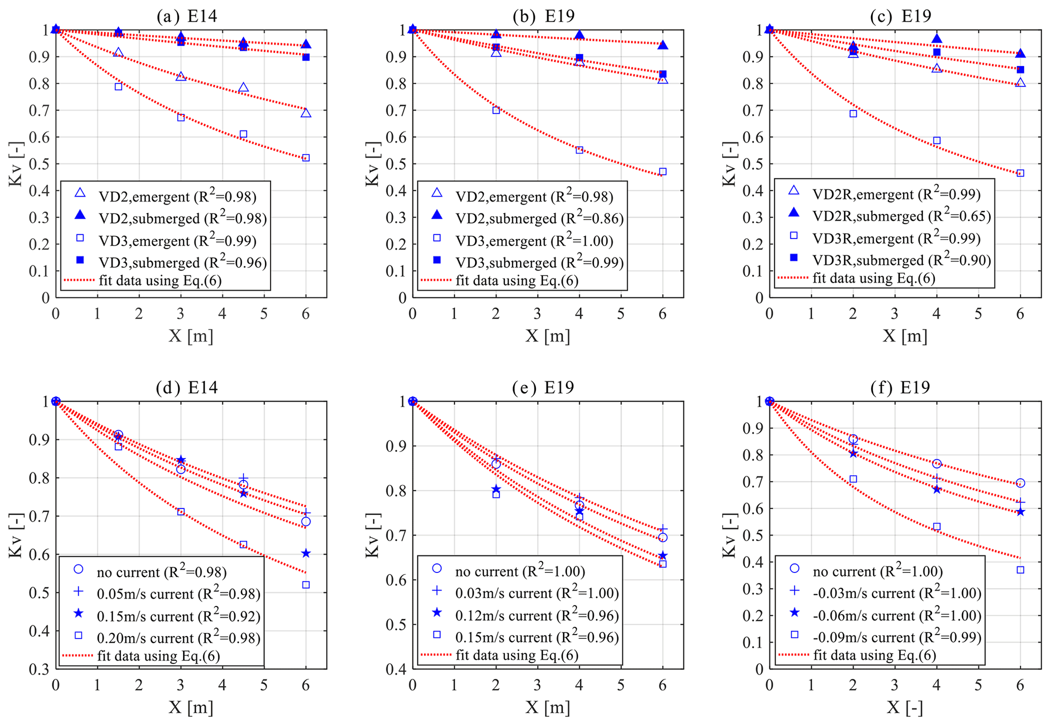
Figure 2Relative wave height (Kv) variation through vegetation canopies (X = 0–6 m). (a) Kv reduction by regular vegetation mimics in pure wave conditions in E14. The tested wave height is 4 cm and the wave period is 1.0 s (i.e., wave0410); (b) Kv reduction by regular vegetation mimics in pure wave conditions in E19. The tested wave condition is wave0308; (c) Kv reduction by randomly disputed vegetation mimics in pure wave conditions in E19. The tested wave condition is wave0308; (d) Kv reduction with following currents in E14. The tested wave condition is wave0410; (e) Kv reduction with following currents in E19. The tested wave condition is wave0510; (f) Kv reduction with opposing currents in E19. The tested wave condition is wave0510. Note the different scale of the Y axis in panels (d)–(f).
2.4 Data analysis
In both experiments, we measured the spatial wave height change, time series of acting force on vegetation mimic (F)T and velocity at the middle water depth (u) as an approximation of the depth-averaged velocity (see Fig. 4). Following the Morison equation (Morison, 1950), F on a vegetation mimic can be specified as
FD and FM are drag force and inertia force, respectively. CM is the inertia coefficient, which value is equal to 2 for cylinders (Dean and Dalrymple, 1991). ρ is the density of water. u is the depth-averaged horizontal flow velocity, and it is assumed to be equal to the flow velocity at half water depth (Hu et al., 2014). Using known u and CD, F can be reproduced by Eq. (1). u can be decomposed as
where ω is the wave angular frequency, and U′ represents turbulent velocity fluctuations, which is neglected in the analysis for simplicity. Umean is the averaged velocity over a wave period (T), defined as (e.g., Pujol et al., 2013)
Please note that Umean is not equal to Uc, which is the imposed current velocity without the influence of waves. Uw is the amplitude of the horizontal wave orbital velocity and can be defined as
where umax and umin are the measured peak flow velocities in the positive and negative directions in a wave period (T). Both umax and umin change with coexisting mean currents. To accommodate empirical KC–CD relations, the KC number is defined as follows (Keulegan and Carpenter, 1958; Chen et al., 2018):
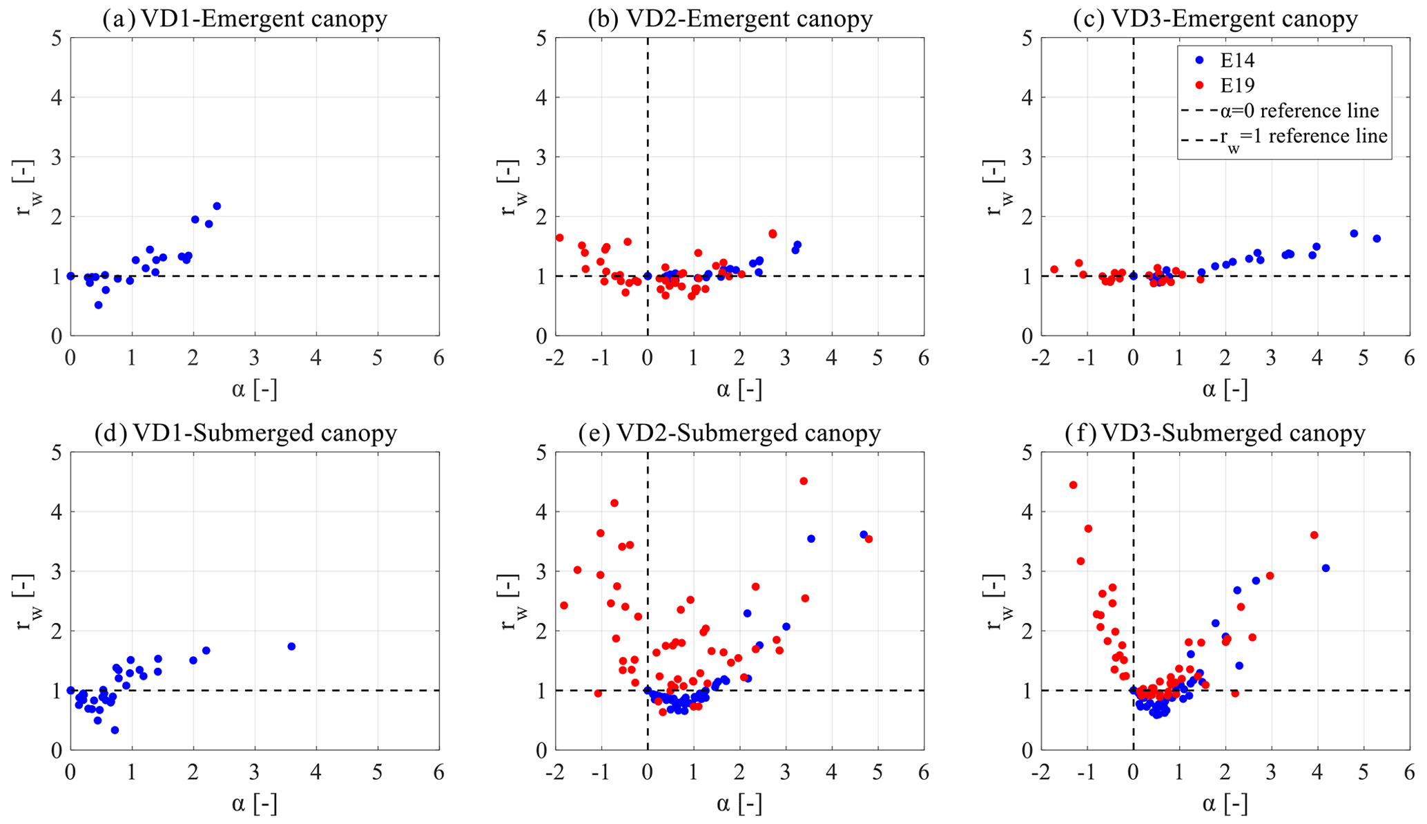
Figure 3Relation between velocity ratios α and the relative decay rw. Panels (a)–(c) show the variation of rw with α in emergent canopies with stem densities of VD1, VD2 and VD3, respectively. Panels (d)–(f) show the variation of rw with α in submerged canopies with stem densities of VD1, VD2 and VD3, respectively. The E14 data points are redrawn from Hu et al. (2014) with permission of Elsevier.
Wave height (H) along the mimic vegetation canopy can be described as
H0 is the wave height at the canopy front. x is the distance into the canopy, and β is a damping coefficient, which can be obtained by fitting Eq. (6). To reveal the effect of coexisting currents, the relative wave height decay in the current–wave and wave-only case rw is defined as
where the Hpw and Hcw are the wave height reduction in pure wave and current–wave cases.
3.1 Wave dissipation in vegetation canopy with following and opposing currents
For pure wave cases, WDV in both experiments has similar variation. Emergent and denser canopies result in greater WDV than submerged and sparser canopies (Figs. 2a and 1b). Additionally, such variation can also be found in the randomly distributed vegetation canopy. No apparent difference can be found between regular and random canopies (Fig. 2c). In waves plus following current cases, the two experiments also show similar results in WDV (Fig. 2d and e). When the following current is small (0.05 m s−1 for E14 and 0.03 m s−1 for E19), the accompany current slightly reduces WDV comparing to the pure wave cases. However, as the following current velocity increases (0.15 m s−1 for E14 and 0.12 m s−1 for E19), WDV is increased compared to the pure wave cases. WDV may be further enhanced by a stronger following current (0.20 m s−1 for E14 and 0.15 m s−1 for E19). As a contrast, opposing currents immediately increase WDV even when the velocity magnitude is small (Fig. 2f). As the opposing current velocity increases, the WDV is promoted to a higher level compared to the cases with the following currents.
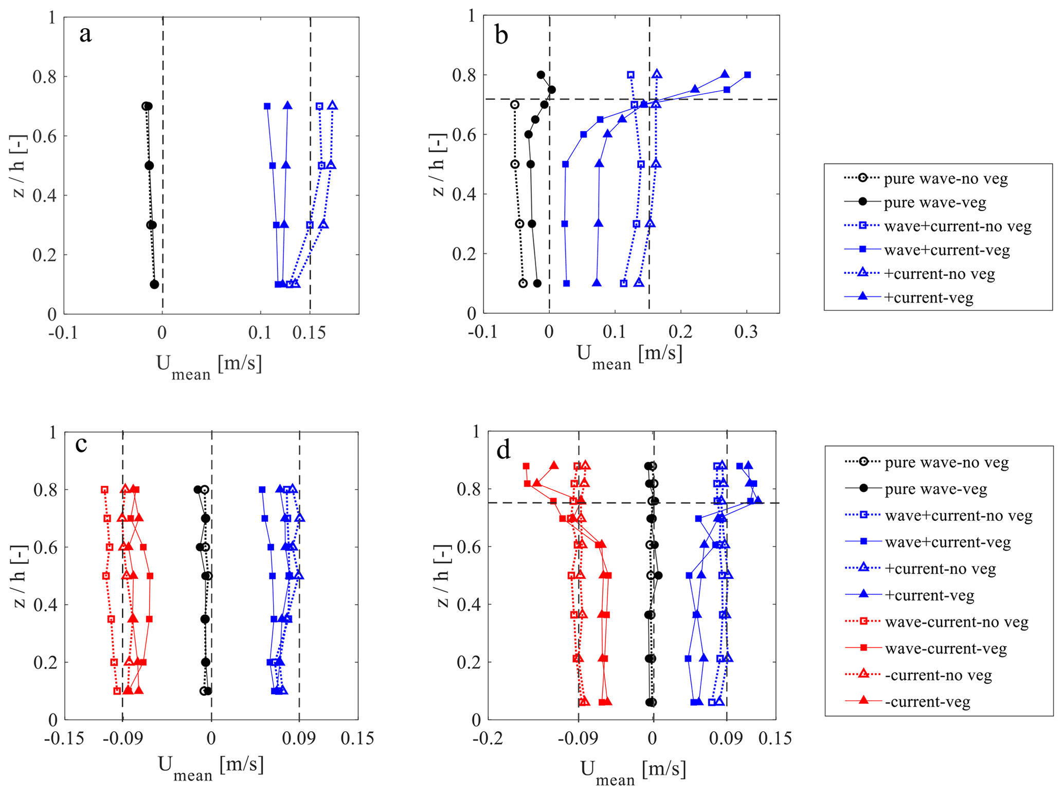
Figure 4Vertical profile of time-mean velocity (Umean). (a) Emergent canopy with incident wave height of 6 cm and wave period of 1.2 s (i.e., wave0612) in E14. The vertical dash lines indicate the imposed current velocities; (b) submerged canopy with case wave1518 in E14. The horizontal line indicates the top of the vegetation canopy; (c) emergent canopy with case wave0508 in E19; (d) submerged canopy with case wave0508 in E19. The E14 data points are redrawn from Hu et al. (2014) with permission from Elsevier.
The results of the two experiments present a synthesis of WDV variation with underlying currents (Fig. 3). In cases with the following currents, the relative wave height decay (rw, ratio of wave height decay between current–wave and wave-only case) has a similar variation in E14 and E19. When α is in the range of [0 1], rw is generally lower than 1; i.e., WDV is suppressed compared to the pure wave cases. As contrast, when α is larger than 1, rw is generally larger than 1, i.e., WDV is enhanced instead. Notably, negative α leads to higher rw compared to positive αwith the same magnitude.Thus, opposing currents can more easily increase WDV compared to the following currents. Notably, rw value can reach 4–5 with both following and opposing currents, highlighting the impact of underlying currents on WDV.
3.2 Velocity and force data
Since the variation of WDV in different flow conditions is closely related to the spatial velocity structures, we measured the vertical velocity profiles in a few tests with the same wave condition but different accompany currents (Fig. 4). Velocity profiles reveal a significant difference in flow structures between cases with various submergence and coexisting current conditions. A few similar patterns can be observed from both experiments: (1) the direction of Umean is determined by the imposed current velocity; (2) in submerged canopies with coexisting currents, a distinctive velocity shear layer can be observed near the top of the vegetation canopy, whereas in emergent canopies velocity profiles are generally uniform; (3) the existence of vegetation reduces Umean magnitude compared to the control VD0 case; (4) when comparing wave-only and wave–current cases, the presence of wave leads to lower Umean magnitude, regardless of the direction of the currents; (5) negative Umean can be found in pure wave conditions, which plays an important role in WDV variation as pointed out in the theoretical model in Hu et al. (2014). The presented velocity profiles are similar to previous experiments (e.g., Li and Yan, 2007; Pujol et al., 2013).
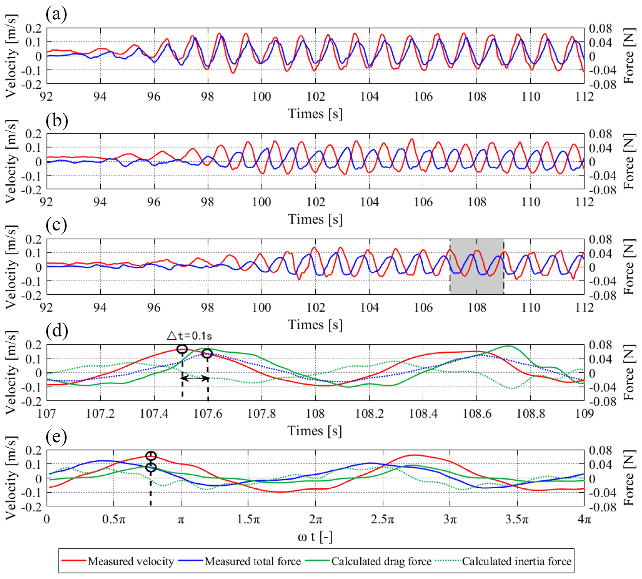
Figure 5Synchronized velocity and force time series. (a–c) Measured raw velocity and total force data at three locations in E19 in the direction of wave propagation; (d) Enlarged data of the shaded area of panel (c), which shows the time shift (t) between u and FD is about 0.1 s. (e) Synchronized u and FD data, which are processed following the method of Yao et al. (2018). The shown test case is with 5 cm wave height, 1.0 s wave period and 0.03 m s−1 following current.
Apart from the vertical velocity structures, we also include the raw data of the temporal variations of velocity (u) and the acting force (F) on vegetation mimics at multiple locations along vegetation canopies to derive CD for all the tested cases (Fig. 5). In each test, velocity and force measurements were taken at the same cross sections. However, time lags still exist between the velocity and force data, which can be perceived via the phase difference between u peak and drag force peak (Fig. 5d). These time lags may be induced by small misalignments between the ADV probes and the force transducers, as well as the intrinsic delays of these instruments. To reduce the time lags and facilitate deriving CD, an automatic algorithm is applied to synchronize u and F data, i.e., reducing the time lags between the peaks of u and FD (Fig. 5e). As a validation of the synchronization, the computed FD (using derived CD) and FM signals are used to compose a reproduced F, which is subsequently compared with the measured total force. A comprehensive comparison shows that the calculated F is consistent with the measured total force (see Fig. C1).
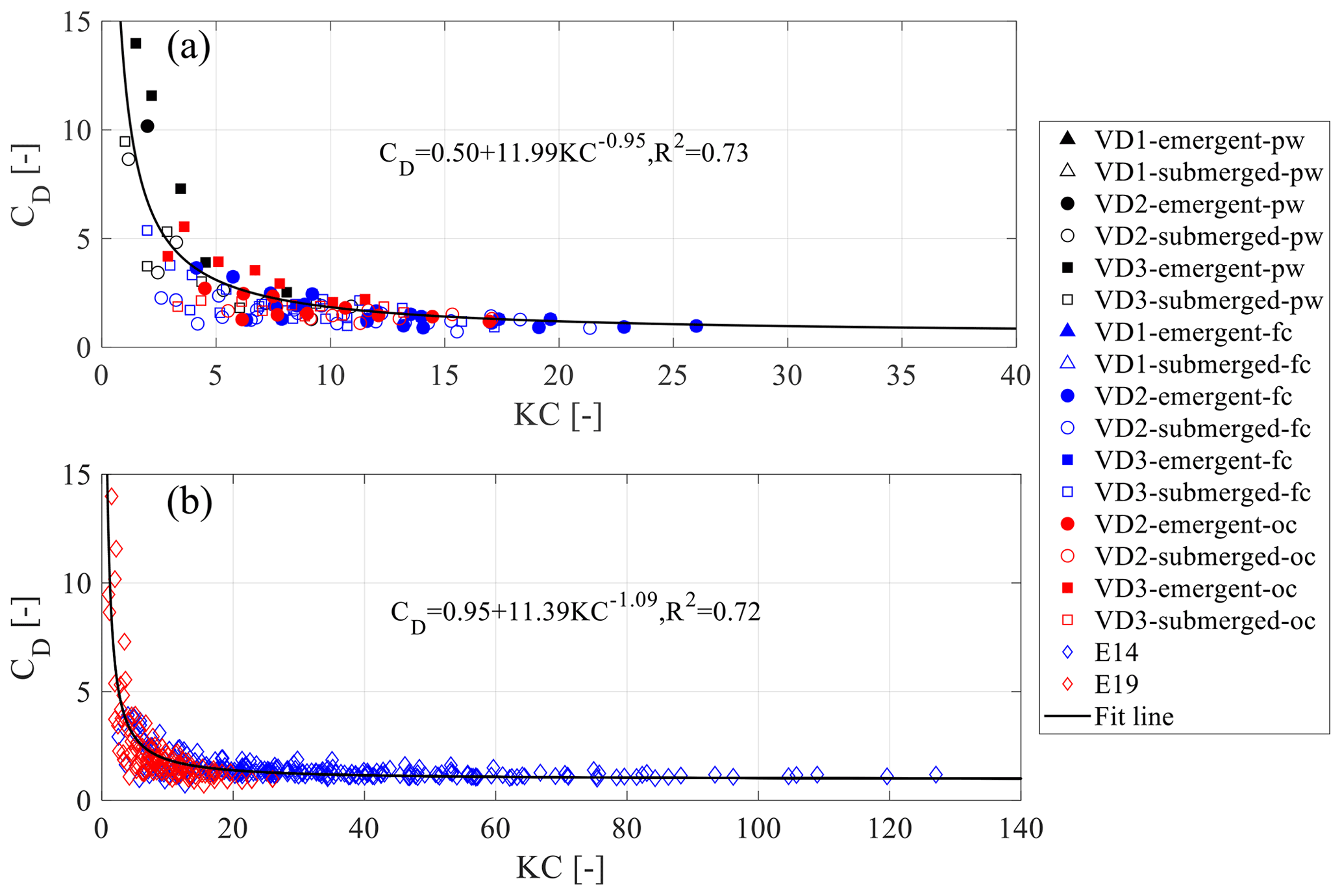
Figure 6Relation between KC and CD. (a) CD in E19 with cases of pure wave (“pw”), wave with following current (“fc”) and wave with opposing current (“oc”); (b) combined CD in both E14 and E19. CD values were derived using the direct measurement approach (Appendix C).
3.3 Drag coefficients
Our combined dataset shows an overall reduction trend of CD with the KC number across all the conditions of vegetation density, submergence ratio and coexisting currents (Fig. 6). In E19, CD reduces fast when KC increases from close to 0 to 10. When the KC number approaches 20, CD is reduced quickly to about 2. As the KC number rises above 20, CD further reduces and finally reaches a nearly constant value of 1.30. It is noted that the variation of CD in opposing currents is similar to that of the following currents. There is no apparent difference between the two experiments, except that E14 contains a wider KC range than E19 (Fig. 6b). A CD–KC relation for combined E14 and E19 data is listed below:
All data presented in this paper are available from figshare (https://doi.org/10.6084/m9.figshare.13026530.v2; Hu et al., 2020). The repository includes data as well as instructions in readme files. Additionally, we expect that the current repository will expand with additional WDV data from ongoing and planned future observation in real mangrove wetlands, e.g., from the ANCODE project (https://www.noc.ac.uk/projects/ancode, last access: 7 October 2021; NOC, 2021).
5.1 Towards a uniform drag coefficient relation
Our dataset includes a wide range of CD in pure wave and wave–current flows. Based on such a dataset, we derived a uniform CD–KC empirical relation covering various combined wave–current conditions with both following and opposing currents. We reveal that CD in opposing currents is also negatively correlated to KC, similar to other flow conditions. The CD data with opposing currents are new supplementary data to the existing studies. The resulting empirical relation can be valuable to the modeling of WDV studies, especially those considering underlying currents. (Henry et al., 2015; Hu et al., 2019; Suzuki et al., 2019; van Veelen et al., 2021). When velocities are unknown to define KC numbers, the velocities may be estimated by linear wave theory or by numerical iterations. For the latter case, an initial CD value can be set as 1 to start the iteration. The current dataset also includes in-canopy velocity, acting force and temporally varying CD. These data can be useful in assessing the force on vegetation stems and estimating, e.g., survival of a mangrove canopy in storm events. Lastly, as our experiments have tested numerous cases with varying canopy density, water depth and current–wave conditions, the generated dataset is thus suitable for machine-learning quests, as such an approach can be capable of deriving more sophisticated relations from multidimensional and nonlinear data (Tinoco et al., 2015; Goldstein et al., 2019).
5.2 A unique dataset for further research in WDV
Our experiments provide a unique dataset of wave height variation through vegetation with coexisting following and opposing currents. It shows that coexisting currents have a substantial impact on WDV. They can reduce WDV by nearly 50 % or increase WDV by 4 times depending on the current velocity ratio (α). Thus, the effect of currents should account for inaccurate WDV assessment. Our data reveal two general patterns of the wave dissipation trend with coexisting currents. First, WDV is suppressed or not sufficiently enhanced when the coexisting current velocity is small, but it is promoted when the current velocity is high, regardless of the imposed velocity direction. Second, in submerged canopies, opposing currents are more likely to promote WDV compared to the following currents. Notably, cases with weak following currents have the lowest WDV in both experiments. Therefore, to ensure safety, these cases should be regarded as the critical condition in designing nature-based coastal defense projects.
For simplicity, the presented dataset does not include tests of flexible vegetation (e.g., salt marshes and seagrass, e.g., Luhar and Nepf, 2011; Maza et al., 2015; van Veelen et al., 2020, 2021) or vegetation with roots or leaves (He et al., 2019; Maza et al., 2019). We expect that the present dataset will expand with additional WDV data in natural mangrove wetlands from ongoing and future observation. While future experiments can certainly benefit from more realistic vegetation characteristics, the current dataset is still valuable in supporting the development of theoretical and numerical models (Losada et al., 2016; Suzuki et al., 2019), as the simplified setting of vegetation canopy facilitates in-depth investigation of complex wave–current–stem interactions. In fact, the CD relation derived in E14 has already been successfully applied in modeling wave dissipation by real flexible marsh plants, i.e., S. anglica, P. maritima and E. athericus (van Veelen et al., 2021). This indicates that the application range of the present dataset is not limited to rigid artificial vegetation but can also be extended to flexible real vegetation. Thus, the present dataset may aid the assessment of the wave dampening capacity and coastal vegetation wetlands as a measure for coastal defense.
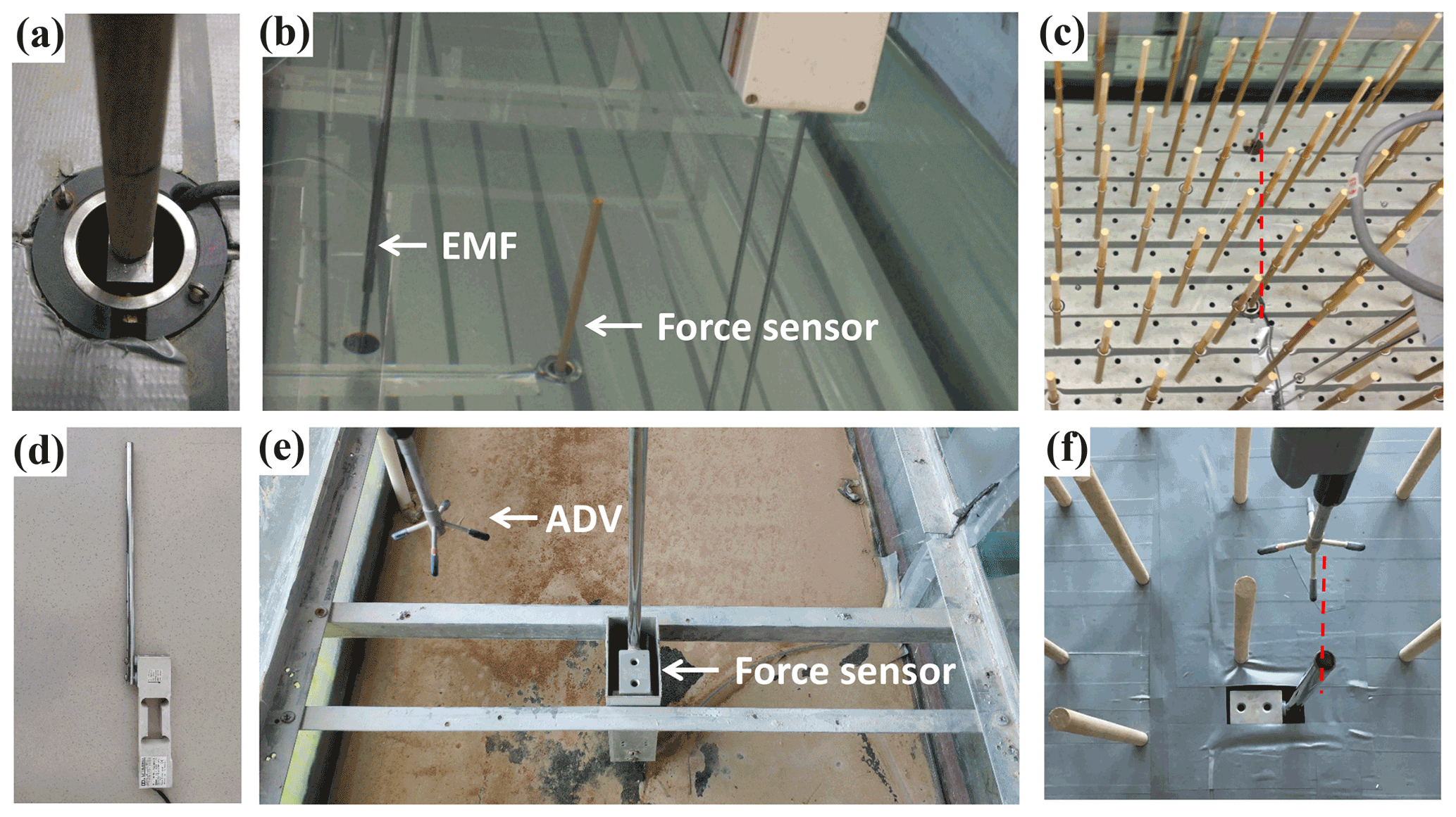
Figure A1Photos of the applied instruments and canopy arrangement in E14 (a–c) and E19 (d–f). In E14, (a) force transducer and (b) EMFs (electromagnetic flow meters) for velocity measurement were developed by Deltares (formerly Delft Hydraulics, the Netherlands). (d) Force transducer (model M104) developed by UTILCELL and (e) ADVs (acoustic Doppler velocimeter) for velocity measurement were from Nortek. Panels (c) and (f) show that the force and velocity measurements were taken at the same transect of the flume to obtain synchronized data.
Table B1 shows the tested cases in both E14 and E19. A large number of tests were included in both experiments: 314 in E14 and 366 in E19. In all the tests, the wave height spatial variation, in-canopy force and velocity were measured. Each test was conducted at least twice to ensure reproducibility. For a few selected cases, the velocity profiles were measured by moving the EMF or ADV measuring probe vertically in the water column.
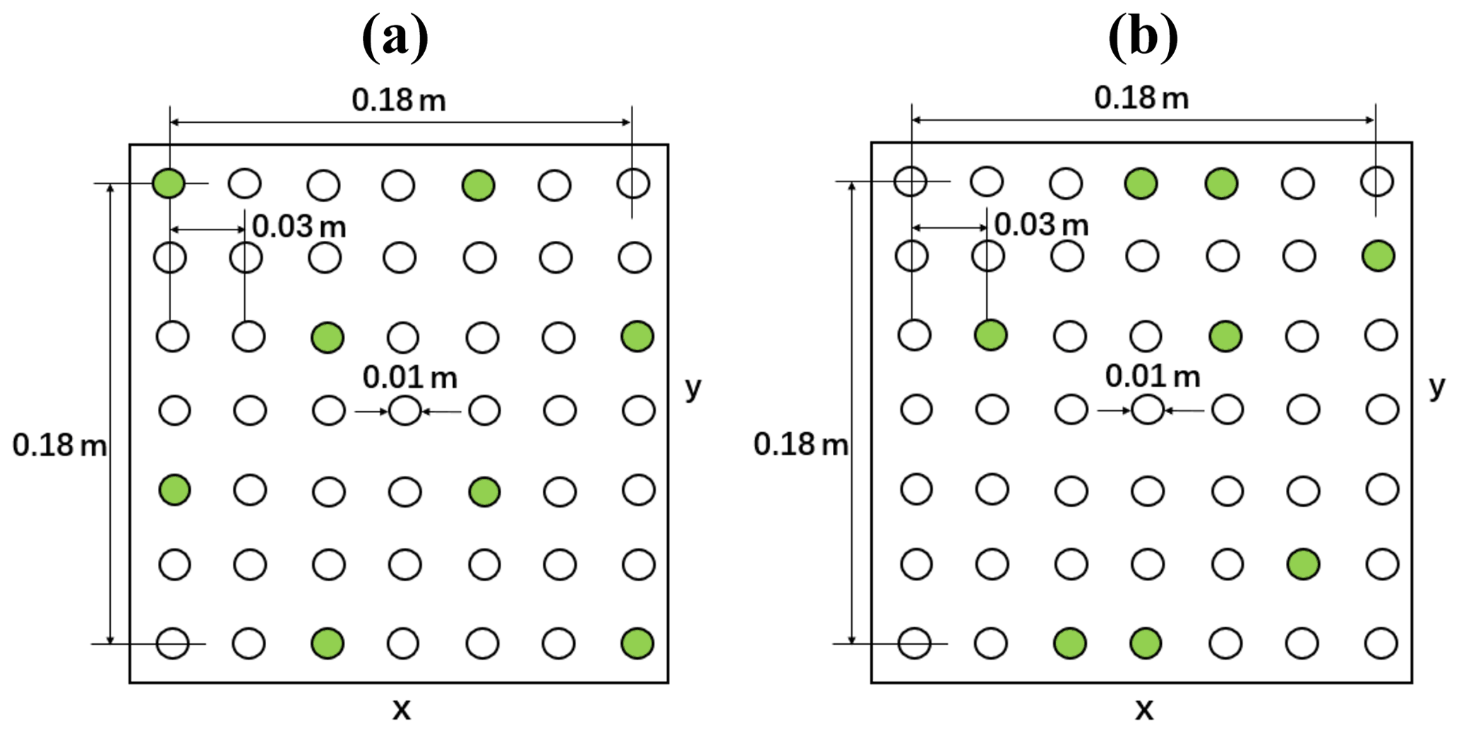
Figure B1Top view of vegetation mimics distribution in E19: (a) regular canopy, 139 stems m−2; (b) random canopy, 139 stems m−2.
In E14, the selected cases were wave0612 and wave1518. For emergent canopy cases (h = 0.25 m), the velocity was measured at four locations: = 0.1, 0.3, 0.5 and 0.7. In submerged canopy cases (h = 0.50 m), u was measured at eight locations: = 0.1, 0.3, 0.5, 0.6, 0.65, 0.75, 0.8 and 0.9. The measuring location was refined near the top of the canopy ( = 0.72). In E19, the selected cases were wave0508. For emergent canopy cases (h = 0.20 m), the velocity was measured at seven locations: = 0.2, 0.3, 0.4, 0.5, 0.65, 0.75 and 0.9. In submerged canopy cases (h = 0.33 m), u was measured at nine locations: = 0.12, 0.18, 0.24, 0.30, 0.39, 0.5, 0.63, 0.79 and 0.94.
Table B1Test conditions in E14 and E19 with different combinations of hydrodynamic conditions and mimic canopy configurations.
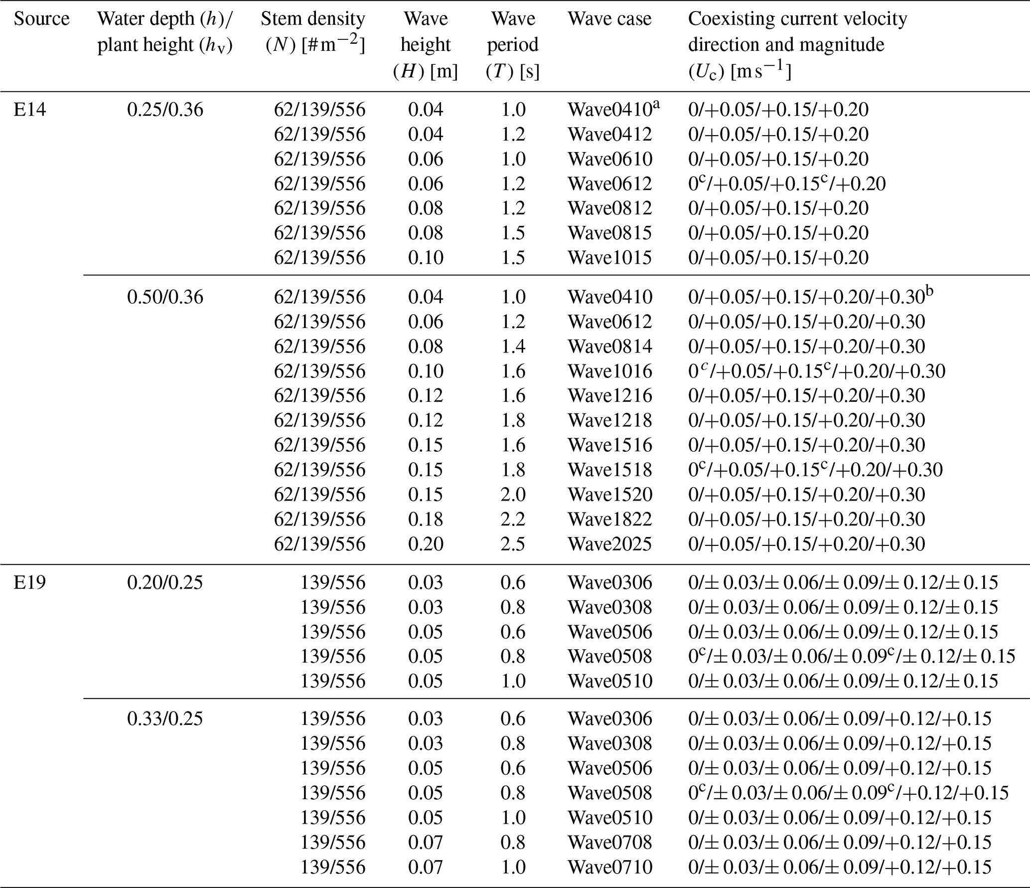
a wave0410 means the incident wave height is 4 cm and the wave period is 1.0 s. b “+” means current flow in the same direction of waves, “−” means current flow in the opposite direction of waves; in E14, the low vegetation density tests (62 stems m−2) does not have “+0.30 m s−1” cases. c in these cases, we conducted velocity profile measurements.
The direct measurement method of CD in combined current–wave flows was first introduced in Hu et al. (2014), and it was further improved in Yao et al. (2018). Such a method is proposed for both pure wave and combined wave–current flows. The force acting on an individual mimic stem is composed of drag force and inertia force, as expressed by the Morison equation (Eq. 1, Morison et al., 1950).
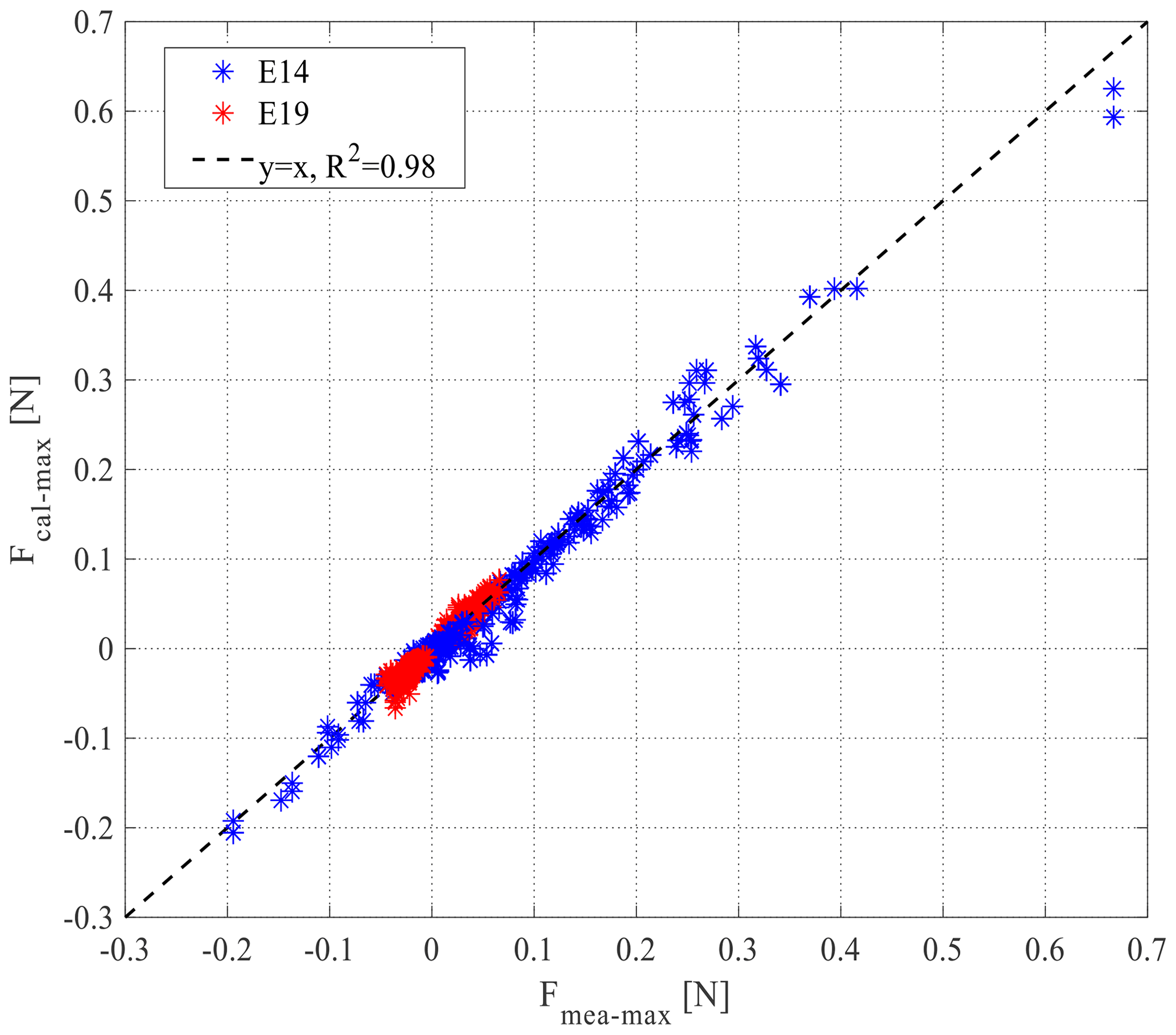
Figure C1A comparison between measured maximum force (Fmea-max) and calculated maximum force (Fcal-max) in both positive and negative directions. Fcal-max is reproduced using directly derived CD.
The only unknown parameter in Morison equation is drag coefficient CD. To derive period-averaged CD, the direct measurement method applies the technique of quantifying the work done by the acting force (Hu et al., 2014). The work done by the acting force on mimic stem over a full wave period is composed of the work done by the drag force and the inertia force, expressed as
where WD and WM are the work performed by FD and FM over a wave period, respectively. Since WM equals to zero in both pure wave and current–wave conditions, FM does not contribute to the WDV (Dalrymple et al., 1984). Hence W equals to WD. Therefore, the period-averaged CD can be derived based on the following equation:
Before applying direct measurement to derive CD, the force data and velocity data should be aligned (Fig. 5d). A detailed procedure of alignment can be found in Yao et al. (2018). As drag force (FD) is a function of velocity (u) Eq. (1), FD and u should be in the same phase. By using measured total force (F), measured velocity (u) and the inertia coefficient (CM) in Eq. (1), we can obtain the drag force (FD) and then adjust the phase shift (Δt) between the velocity and drag force peaks. The obtained new velocity and force data time series are used as inputs in the next run. This loop is executed over 30 times. Finally, the minimum phase shift (Δt) and the aligned velocity and force time series are chosen as outputs for deriving CD. As a validation of the directly derived CD, we reproduced the maximum force (Fcal-max) in both positive and negative directions using the derived CD and compared it with the measured maximum force (Fmea-max; see Fig. C1).
ZH, LS, HW and YL conducted the experiments and collected the raw data. ZH, MS and TS designed the experiments. ZH, LS and YL prepared the manuscript with contributions from all authors.
The contact author has declared that neither they nor their coauthors have any competing interests.
Publisher's note: Copernicus Publications remains neutral with regard to jurisdictional claims in published maps and institutional affiliations.
We would like to thank Yan Ni, Tjerk Zitman, Wim Uijttewaal, Maike Paul, Hong Wang, Lei Ren and Hui Chen for supporting our experiments.
This work is supported by the ANCODE (Applying nature-based coastal defense to the world’s largest urban area – from science to practice) project, three-way international funding through the Chinese National Natural Science Foundation (NSFC, grant no. 51761135022), the Netherlands Organization for Scientific Research (NWO, lead funder, grant no. ALWSD.2016.026), the UK research councils (EPSRC, grant no. EP/R024537/1), the Innovation Group Project of the Southern Marine Science and Engineering Guangdong Laboratory (Zhuhai) (grant no. 311021004), Fundamental Research Funds for the Central Universities of China (grant no. 20lgzd16), the Guangdong Provincial Department of Science and Technology (grant no. 2019ZT08G090), and the 111 Project (grant no. B21018).
This paper was edited by Giuseppe M. R. Manzella and reviewed by two anonymous referees.
Anderson, M. E. and Smith, J. M.: Wave attenuation by flexible, idealized salt marsh vegetation, Coast. Eng., 83, 82–92, https://doi.org/10.1016/j.coastaleng.2013.10.004, 2014.
Arkema, K. K., Griffin, R., Maldonado, S., Silver, J., Suckale, J., and Guerry, A. D.: Linking social, ecological, and physical science to advance natural and nature-based protection for coastal communities, Ann. NY Acad. Sci., 1399, 5–26, https://doi.org/10.1111/nyas.13322, 2017.
Augustin, L. N., Irish, J. L., and Lynett, P.: Laboratory and numerical studies of wave damping by emergent and near-emergent wetland vegetation, Coast. Eng., 56, 332–340, 2009.
Borsje, B. W., Vries, S. de, Janssen, S. K. H., Luijendijk, A. P., and Vuik, V.: Building with nature as coastal protection strategy in the Netherlands, in: Living shorelines: The science and management of nature-based coastal protection, edited by: Bilkovic, D. M., Mitchell, M. M., La Peyre, M. K., and Toft, J. D., CRC Press, New York, 137–156, 2017.
Bouma, T. J., De Vries, M. B., Low, E., Peralta, G., Tánczos, I. C., Van De Koppel, J., and Herman, P. M. J.: Trade-offs related to ecosystem engineering: A case study on stiffness of emerging macrophytes, Ecology, 86, 2187–2199, 2005.
Cao, H., Feng, W., Hu, Z., Suzuki, T., and Stive, M. J. F.: Numerical modeling of vegetation-induced dissipation using an extended mild-slope equation, Ocean Eng., 110, 258–269, https://doi.org/10.1016/j.oceaneng.2015.09.057, 2015.
Chen, H., Ni, Y., Li, Y., Liu, F., Ou, S., Su, M., Peng, Y., Hu, Z., Uijttewaal, W., and Suzuki, T.: Deriving vegetation drag coefficients in combined wave-current flows by calibration and direct measurement methods, Adv. Water Resour., 122, 217–227, https://doi.org/10.1016/j.advwatres.2018.10.008, 2018.
Currin, C. A.: Living Shorelines for Coastal Resilience, Chapter 30, in: Coastal Wetlands, edited by: Perillo, G. M. E., Wolanski, E., Cahoon, D. R., and Hopkinson, C. S., Elsevier, Amsterdam, 1023–1053, https://doi.org/10.1016/B978-0-444-63893-9.00030-7, 2019.
Dalrymple, R., Kirby, J., and Hwang, P.: Wave Diffraction Due to Areas of Energy Dissipation, Journal of Waterway, Port, Coastal, and Ocean Engineering, 110, 67–79, https://doi.org/10.1061/(ASCE)0733-950X(1984)110:1(67), 1984.
Dean, R. and Dalrymple, R.: Water Wave Mechanics for Engineers and Scientists, World Scientific, Tokyo, 1991.
Delft Hydraulics: User's manual for the delft hydraulics four quadrant electromagnetic liquid, Delft, the Netherlands, 1990.
Delft Hydraulics: Manual for Wave Height Meter, Delft, the Netherlands, p. 2, year unknown.
Demirbilek, Z., Dalrymple, R. A., Sorenson, R. M., Thompson, E. F., and Weggel, J. R.: Water waves, in: Hydrology Handbook, edited by: Heggen, R. J., ASCE, New York, 627–720, 1996.
Garzon, J. L., Maza, M., Ferreira, C. M., Lara, J. L., and Losada, I. J.: Wave Attenuation by Spartina Saltmarshes in the Chesapeake Bay Under Storm Surge Conditions, J. Geophys. Res.-Oceans, 124, 5220–5243, https://doi.org/10.1029/2018JC014865, 2019.
Goldstein, E. B., Coco, G., and Plant, N. G.: A review of machine learning applications to coastal sediment transport and morphodynamics, Earth-Sci. Rev., 194, 97–108, https://doi.org/10.1016/j.earscirev.2019.04.022, 2019.
He, F., Chen, J., and Jiang, C.: Surface wave attenuation by vegetation with the stem, root and canopy, Coast. Eng., 152, 103509, https://doi.org/10.1016/j.coastaleng.2019.103509, 2019.
Henry, P.-Y., Myrhaug, D., and Aberle, J.: Drag forces on aquatic plants in nonlinear random waves plus current, Estuar. Coast. Shelf S., 165, 10–24, https://doi.org/10.1016/j.ecss.2015.08.021, 2015.
Hu, J., Hu, Z., and Liu, P. L.-F.: Surface water waves propagating over a submerged forest, Coast. Eng., 152, 103510, https://doi.org/10.1016/j.coastaleng.2019.103510, 2019.
Hu, Z., Suzuki, T., Zitman, T., Uijttewaal, W., and Stive, M.: Laboratory study on wave dissipation by vegetation in combined current-wave flow, Coast. Eng., 88, 131–142, https://doi.org/10.1016/j.coastaleng.2014.02.009, 2014.
Hu, Z., Lian, S., Wei, H., Li, Y., Uijttewaal, W., and Suzuki, T.: A dataset on wave propagation through vegetation with coexisting currents, figshare, Dataset, https://doi.org/10.6084/m9.figshare.13026530.v2, 2020.
Hudspeth, R. T. and Sulisz, W.: Stokes drift in two-dimensional wave flumes, J. Fluid Mech., 230, 209–229, https://doi.org/10.1017/S0022112091000769, 1991.
Jadhav, R. S., Chen, Q., and Smith, J. M.: Spectral distribution of wave energy dissipation by salt marsh vegetation, Coast. Eng., 77, 99–107, https://doi.org/10.1016/j.coastaleng.2013.02.013, 2013.
Koftis, T., Prinos, P., and Stratigaki, V.: Wave damping over artificial Posidonia oceanica meadow: A large-scale experimental study, Coast. Eng., 73, 71–83, https://doi.org/10.1016/j.coastaleng.2012.10.007, 2013.
Keulegan, G. H. and Carpenter, L. H.: Forces on cylinders and plates in an oscillating fluid, J. Res. Nat. Bur. Stand., 60, 423–440, 1958.
Lara, J. L., Maza, M., Ondiviela, B., Trinogga, J., Losada, I. J., Bouma, T. J., and Gordejuela, N.: Large-scale 3-D experiments of wave and current interaction with real vegetation. Part 1: Guidelines for physical modeling, Coast. Eng., 107, 70–83, https://doi.org/10.1016/j.coastaleng.2015.09.012, 2016.
Lei, J. and Nepf, H.: Blade dynamics in combined waves and current, J. Fluid. Struct., 87, 137–149, https://doi.org/10.1016/j.jfluidstructs.2019.03.020, 2019.
Leonardi, N., Camacina, I., Donatelli, C., Ganju, N. K., Plater, A. J., Schuerch, M., and Temmerman, S.: Dynamic interactions between coastal storms and salt marshes: A review, Geomorphology, 301, 92–107, https://doi.org/10.1016/j.geomorph.2017.11.001, 2018.
Li, C. W. and Yan, K.: Numerical investigation of Wave–Current–Vegetation interaction, J. Hydraul. Eng., 133, 794–803, https://doi.org/10.1061/(ASCE)0733-9429(2007)133:7(794), 2007.
Losada, I. J., Maza, M., and Lara, J. L.: A new formulation for vegetation-induced damping under combined waves and currents, Coast. Eng., 107, 1–13, https://doi.org/10.1016/j.coastaleng.2015.09.011, 2016.
Maza, M., Lara, J. L., Losada, I. J., Ondiviela, B., Trinogga, J., and Bouma, T. J.: Large-scale 3-D experiments of wave and current interaction with real vegetation. Part 2: Experimental analysis, Coast. Eng., 106, 73–86, https://doi.org/10.1016/j.coastaleng.2015.09.010, 2015.
Maza, M., Lara, J. L., and Losada, I. J.: Experimental analysis of wave attenuation and drag forces in a realistic fringe Rhizophora mangrove forest, Adv. Water Resour., 131, 103376, https://doi.org/10.1016/j.advwatres.2019.07.006, 2019.
Méndez, F. J. and Losada, I. J.: An empirical model to estimate the propagation of random breaking and nonbreaking waves over vegetation fields, Coast. Eng., 51, 103–118, 2004.
Möller, I., Kudella, M., Rupprecht, F., Spencer, T., Paul, M., van Wesenbeeck, B. K., Wolters, G., Jensen, K., Bouma, T. J., Miranda-Lange, M., and Schimmels, S.: Wave attenuation over coastal salt marshes under storm surge conditions, Nat. Geosci., 7, 727–731, https://doi.org/10.1038/ngeo2251, 2014.
Morison, J. R., Johnson, J. W., and Schaaf, S. A.: The Force Exerted by Surface Waves on Piles, J. Petrol. Technol., 2, 149–154, https://doi.org/10.2118/950149-G, 1950.
Nepf, H. M.: Flow Over and Through Biota, in: Treatise on Estuarine and Coastal Science, edited by: Wolanski, E. and McLusky, D., Academic Press, Waltham, 267–288, 2011.
NOC: ANCODE project, NOC (National Oceanography Centre), available at: https://www.noc.ac.uk/projects/ancode, last access: 7 October 2021.
Ota, T., Kobayashi, N., and Kirby, J. T.: Wave and current interactions with vegetation, in: Proceedings of the 29th International Conference on Coastal Engineering, Coastal Engineering 2004, National Civil Engineering Laboratory, Lisbon, Portugal, 508–520, https://doi.org/10.1142/9789812701916_0040, 2005.
Ozeren, Y., Wren, D. G., and Wu, W.: Experimental investigation of wave attenuation through model and live vegetation, Journal of Waterway, Port, Coastal, and Ocean Engineering, 140, https://doi.org/10.1061/(ASCE)WW.1943-5460.0000251, 2014.
Paul, M., Bouma, T. J., and Amos, C. L.: Wave attenuation by submerged vegetation: combining the effect of organism traits and tidal current, Mar. Ecol. Prog. Ser., 444, 31–41, https://doi.org/10.3354/meps09489, 2012.
Pujol, D., Serra, T., Colomer, J., and Casamitjana, X.: Flow structure in canopy models dominated by progressive waves, J. Hydrol., 486, 281–292, https://doi.org/10.1016/j.jhydrol.2013.01.024, 2013.
Stewart, H. L.: Hydrodynamic consequences of maintaining an upright posture by different magnitudes of stiffness and buoyancy in the tropical alga Turbinaria ornata, J. Marine Syst., 49, 157–167, https://doi.org/10.1016/j.jmarsys.2003.05.007, 2004.
Stratigaki, V., Manca, E., Prinos, P., Losada, I. J., Lara, J. L., Sclavo, M., Amos, C. L., Cáceres, I., and Sánchez-Arcilla, A.: Large-scale experiments on wave propagation over Posidonia oceanica, J. Hydraul. Res., 49, 31–43, https://doi.org/10.1080/00221686.2011.583388, 2011.
Suzuki, T., Hu, Z., Kumada, K., Phan, L. K., and Zijlema, M.: Non-hydrostatic modeling of drag, inertia and porous effects in wave propagation over dense vegetation fields, Coast. Eng., 149, 49–64, https://doi.org/10.1016/j.coastaleng.2019.03.011, 2019.
Temmerman, S., Meire, P., Bouma, T. J., Herman, P. M. J., Ysebaert, T., and De Vriend, H. J.: Ecosystem-based coastal defence in the face of global change, Nature, 504, 79–83, https://doi.org/10.1038/nature12859, 2013.
Tinoco, R. O., Goldstein, E. B., and Coco, G.: A data-driven approach to develop physically sound predictors: Application to depth-averaged velocities on flows through submerged arrays of rigid cylinders, Water Resour. Res., 51, 1247–1263, https://doi.org/10.1002/2014WR016380, 2015.
Tinoco, R. O., San Juan, J. E., and Mullarney, J. C.: Simplification bias: lessons from laboratory and field experiments on flow through aquatic vegetation, Earth Surf. Proc. Land., 45, 121–143, https://doi.org/10.1002/esp.4743, 2020.
van Loon-Steensma, J. M., Slim, P. A., Decuyper, M., and Hu, Z.: Salt-marsh erosion and restoration in relation to flood protection on the Wadden Sea barrier island Terschelling, J. Coast. Conserv., 1–16, https://doi.org/10.1007/s11852-014-0326-z, 2014.
van Loon-Steensma, J. M., Hu, Z., and Slim, P. A.: Modelled Impact of Vegetation Heterogeneity and Salt-Marsh Zonation on Wave Damping, J. Coastal Res., 32, 241–252, https://doi.org/10.2112/JCOASTRES-D-15-00095.1, 2016.
van Veelen, T. J., Fairchild, T. P., Reeve, D. E., and Karunarathna, H.: Experimental study on vegetation flexibility as control parameter for wave damping and velocity structure, Coast. Eng., 157, 103648, https://doi.org/10.1016/j.coastaleng.2020.103648, 2020.
van Veelen, T. J., Karunarathna, H., and Reeve, D. E.: Modelling wave attenuation by quasi-flexible coastal vegetation, Coast. Eng., 164, 103820, https://doi.org/10.1016/j.coastaleng.2020.103820, 2021.
Vuik, V., Jonkman, S. N., Borsje, B. W., and Suzuki, T.: Nature-based flood protection: The efficiency of vegetated foreshores for reducing wave loads on coastal dikes, Coast. Eng., 116, 42–56, https://doi.org/10.1016/j.coastaleng.2016.06.001, 2016.
Yao, P., Chen, H., Huang, B., Tan, C., Hu, Z., Ren, L., and Yang, Q.: Applying a New Force-Velocity Synchronizing Algorithm to Derive Drag Coefficients of Rigid Vegetation in Oscillatory Flows, Water, 10, 906, https://doi.org/10.3390/w10070906, 2018.
- Abstract
- Introduction
- Methods
- Data
- Data availability
- Recommendations for data reuse
- Appendix A: Photos of the experiment instruments and setup
- Appendix B: Test conditions in the two experiments
- Appendix C: Direct measurement method of CD
- Author contributions
- Competing interests
- Disclaimer
- Acknowledgements
- Financial support
- Review statement
- References