the Creative Commons Attribution 4.0 License.
the Creative Commons Attribution 4.0 License.
 | 15 Feb 2021
Climate benchmarks and input parameters representing locations in 68 countries for a stochastic weather generator, CLIGEN
Andrew T. Fullhart
Mark A. Nearing
Gerardo Armendariz
Mark A. Weltz
This dataset contains input parameters for 12 703 locations around the world to parameterize a stochastic weather generator called CLIGEN. The parameters are essentially monthly statistics relating to daily precipitation, temperature, and solar radiation. The dataset is separated into three sub-datasets differentiated by having monthly statistics determined from 30-, 20-, and 10-year record lengths. Input parameters related to precipitation were calculated primarily from the NOAA GHCN-Daily network. The remaining input parameters were calculated from various sources including global meteorological and land-surface models that are informed by remote sensing and other methods. The new CLIGEN dataset includes inputs for locations in the US, which were compared to a selection of stations from an existing US CLIGEN dataset representing 2648 locations. This validation showed reasonable agreement between the two datasets, with the majority of parameters showing less than 20 % discrepancy relative to the existing dataset. For the three new datasets, differentiated by the minimum record lengths used for calculations, the validation showed only a small increase in discrepancy going towards shorter record lengths, such that the average discrepancy for all parameters was greater by 5 % for the 10-year dataset. The new CLIGEN dataset has the potential to improve the spatial coverage of analysis for a variety of CLIGEN applications and reduce the effort needed in preparing climate inputs. The dataset is available at the National Agriculture Library Data Commons website at https://data.nal.usda.gov/dataset/international-climate-benchmarks-and-input-parameters-stochastic-weather-generator-cligen (last access: 20 November 2020) and https://doi.org/10.15482/USDA.ADC/1518706 (Fullhart et al., 2020a).
- Article
(1125 KB) - Full-text XML
- BibTeX
- EndNote


Essential climate variables defined by the World Meteorological Organization are physical, chemical, or biological variables, or groups of linked variables that critically contribute to the characterization of Earth's climate (Bojinski et al., 2014). Aside from their use in climate studies, basic essential climate variables like precipitation and temperature are important for water resource management, drought monitoring, agricultural engineering, and other applications (Hollmann et al., 2013). The temporal resolution of climate data varies for these applications. Climate data reduced to monthly statistics may facilitate analysis of multi-decadal climate trends and serve as benchmarks of climate normals (Menne et al., 2012; Hollmann et al., 2013). In this paper, it is discussed how a stochastic weather generator may be parameterized with a new dataset of monthly climate statistics to simulate daily weather outputs for locations around the world.
Stochastic weather generators are used for a variety of applications that include model forcing, statistical downscaling of climate models, and study of climate change scenarios (Vaghefi and Yu, 2017). CLImate GENerator (CLIGEN) is one such point-scale weather generator that produces daily outputs based on input parameters that are essentially observed monthly statistics. CLIGEN is regularly used to provide soil erosion models with realistic trends and statistical distributions of weather parameters (Kinnell, 2019). Such models include the Rangeland Hydrology and Erosion Model (RHEM), the Water Erosion Prediction Project (WEPP) model, and the Revised Universal Soil Loss Equation 2 (RUSLE 2) model. CLIGEN can generate long-term realizations of stationary climate, subsequently enabling long-term erosion simulations and ensuring that average annual erosion rates reach convergence (Baffaut et al., 1996). CLIGEN has been validated in a number of countries, under a variety of climates, and for different outputs that include daily precipitation, peak intensity, time-to-peak intensity, storm duration, and storm frequency. For example, Mehan et al. (2017) showed that the mean of all daily precipitation values was within 0.1 mm of observations, and minimum and maximum daily temperatures were within 0.1 ∘C for locations in the western Lake Erie basin. A particularly important CLIGEN output is precipitation intensity because of its high model sensitivity in erosion and runoff modeling (Nearing et al., 2005). Zhang et al. (2008) validated intensity for the loess plateau of China based on distributions of maximum 30 min intensities (I30) that were derived from CLIGEN's peak intensity. They found that differences with observed distributions were statistically insignificant, suggesting that rainfall erosivity could be accurately estimated using CLIGEN.
CLIGEN has location-specific input parameters for the United States with dense coverage, but on a global scale, input parameters are sparsely available. This is partly because of the labor-intensive nature of determining the parameters and because of numerous data requirements, e.g., high-frequency precipitation measurements. For erosion modeling, the lack of widely available CLIGEN inputs has hindered progress towards increasing the spatial scale and coverage of analysis that other aspects of soil erosion research have brought to the global scale, one example being the development of global maps of annual rainfall erosivity (Panagos et al., 2017). Hence, in the interest of increasing the availability of CLIGEN inputs for soil erosion modeling and other applications, we present a dataset of CLIGEN input parameter files. The dataset represents 12 703 locations in 68 countries. Besides providing the necessary parameters to run CLIGEN simulations, the dataset also serves to provide statistics for representing climate normals. The parameters are validated using an existing CLIGEN input dataset for the United States, and differences are discussed.
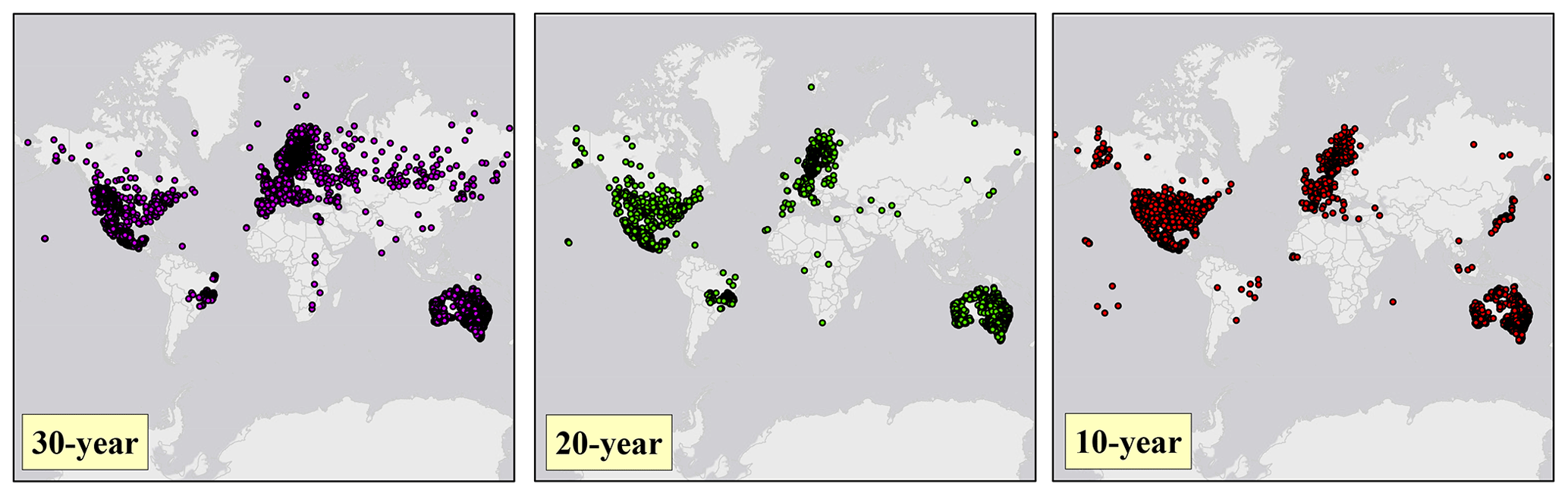
Figure 1Coverage of the three international CLIGEN input datasets according to the record length used to produce the monthly input parameters. The locations correspond to those of the GHCN-Daily stations accepted for use.
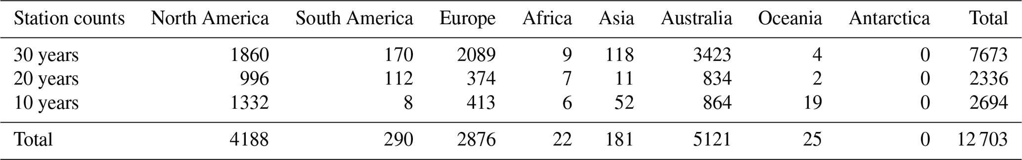
Table 1Station counts for continent/region and each of the 30-, 20-, and 10-year datasets. Oceania is the region represented by South Pacific islands and extending north to Hawaii.
2.1 Overview
Three sets of CLIGEN v5.3 input files for international locations are presented, differentiated by having monthly parameters determined from minimums of 30-, 20-, and 10-year records (note that assumptions were made to handle data gaps which are discussed in Sect. 2.2) (Fullhart et al., 2020a). The distribution of locations for the three datasets is in Fig. 1, which shows 7673 parameter sets based on 30-year records (left panel), 2336 parameter sets based on 20-year records (middle panel), and 2694 parameter sets based on 10-year records (right panel). All locations are unique, with no overlap in locations between the three datasets. As may be seen in Fig. 1, there is relatively sparse coverage for South America, Africa, and southern Asia, while North America, Europe, and Australia have relatively dense coverage. The spatial density of all stations is shown in Fig. 2 so that density may be judged in places where overcrowding of points occurs in Fig. 1, and Table 1 enumerates the number of stations on each continent. Furthermore, a .kmz map layer is available on the Ag Data Commons website (link given in Sect. 4) that can be imported into Google Earth as an interactive map and allows the CLIGEN station closest to an area of interest to be found.

Figure 2Station density map representing all stations combined. The cell size is defined by lat–long degree lines (1∘ × 1∘). Densities are calculated inside of circular neighborhoods with radii of 3∘ from the center of each cell.
As 30 years is traditionally the minimum record length needed to represent climate, the 30-year dataset may be used to characterize climate normals (Bojinski et al., 2014). The 20- and 10-year datasets, reflecting the most recent monthly records available at each location, may be more representative of current climates in some cases considering the non-stationarity of current and projected climate conditions (IPCC, 2013). In soil erosion modeling, a 20-year record has been suggested as the minimum length needed to represent rainfall erosivity (Wischmeier and Smith, 1978), which may be estimated using CLIGEN (Lobo et al., 2015). It should be noted that in non-stationary climates, CLIGEN inputs may be adjusted to represent departures from climate normals (Pruski and Nearing, 2002; Zhang, 2005; Vaghefi and Yu, 2016). For example, Zhang (2013) determined how CLIGEN's precipitation intensity and skewness factors scale with monthly precipitation to correct for future changes in precipitation.
Table 2A list of CLIGEN input parameters determined for each station. The temporal resolution column indicates the resolution of the data used to derive each parameter. Parameters that require sub-daily resolutions at various frequencies of measurement are denoted with “High-res” in the temporal resolution column. Sub-daily resolution data were not available for High-res. parameters, and it is discussed how their values were estimated.
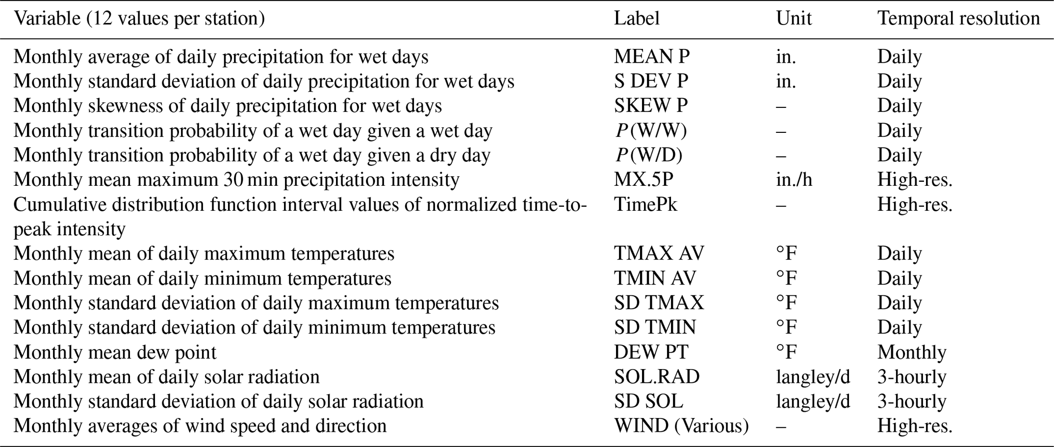
A list of parameters and their definitions that were determined for each input file is given in Table 2. These parameters are used to model statistical distributions that are randomly sampled by CLIGEN to derive daily outputs. Some parameters such as TMAX AV and TMIN AV (refer to Table 2 for definitions) are also typical climate benchmarks. Another climate benchmark, average monthly precipitation, may be determined by the following calculation from input parameters:
where n is the number of calendar days in the month being considered, and Pavg is the MEAN P CLIGEN parameter.
The various input parameters were derived from an assortment of data sources. In general, there were two main categories of sources: (1) ground-based precipitation networks, and (2) land-surface and meteorological models that assimilate remote sensing data and ground observations and which reproduce historical time series of variables of concern. The sources of data had various temporal resolutions. In most cases, the data were used to make direct calculation of parameters, but for parameters where the available data were insufficient for direct calculation, parameter estimations were done. Each data source and the resulting parameters are discussed in detail in the following sections.
2.2 Precipitation accumulation
The primary source of precipitation data is the Global Historical Climate Network-Daily (GHCN-Daily) maintained by NOAA (Menne et al., 2012). The locations shown in Fig. 1 correspond to those of selected stations from GHCN-Daily. These ground-based records enabled direct calculation of five parameters related to precipitation accumulation: MEAN P, S DEV P, SKEW P, , and (see Table 2 for their definitions). The GHCN-Daily dataset undergoes rigorous quality control, both to check for consistency of formatting and for the integrity of daily values. Values are removed that fail any test in a suite of quality tests which identify a variety of problems. Durre et al. (2010) outlined 19 of the quality tests in detail.
Short record lengths and missing data precluded a wide majority (∼90 %) of GHCN-Daily stations from being used to create CLIGEN input parameters. A substantial number of data gaps necessitated an assumption for the calculation of the five monthly parameters related to accumulation. To handle gaps, records were queried starting with the most recent year available and going backwards in each time series until the number of months needed could be produced by replacing gaps with existing records from earlier in the time series. Therefore, it was assumed that time series do not need to be temporally continuous. This means that records were accepted which did not necessarily come from sequential months, but which had at least 30, 20, and 10 complete individual months for each calendar month, in order to derive the 30-, 20-, and 10-year monthly statistics, respectively. As a result, record lengths were queried that were often longer than the number of years needed. Also, since representing recent data was a priority, 96 % of stations included at least some data after the year 2000, and 81 % included some data after the year 2010. Ranges of years queried for each station are given in an extensive table available on the Ag Data Commons website (link given in Sect. 4). The ranges are defined by the first and last years with at least one monthly record accepted for use. Ranges in excess of the 30-, 20-, and 10-year minimum record lengths are due to data gaps for respective datasets. The longest viable record length (of 30, 20, and 10 years) was used for each station, such that if a 30-year record was possible, 10- and 20-year records were not created. Therefore, no stations have multiple datasets created for them. This treatment of data gaps complicates the validation of the determined climate benchmarks against other datasets with similar temporal ranges, and the effect of non-stationarity and long-term climate cycles should also be considered.
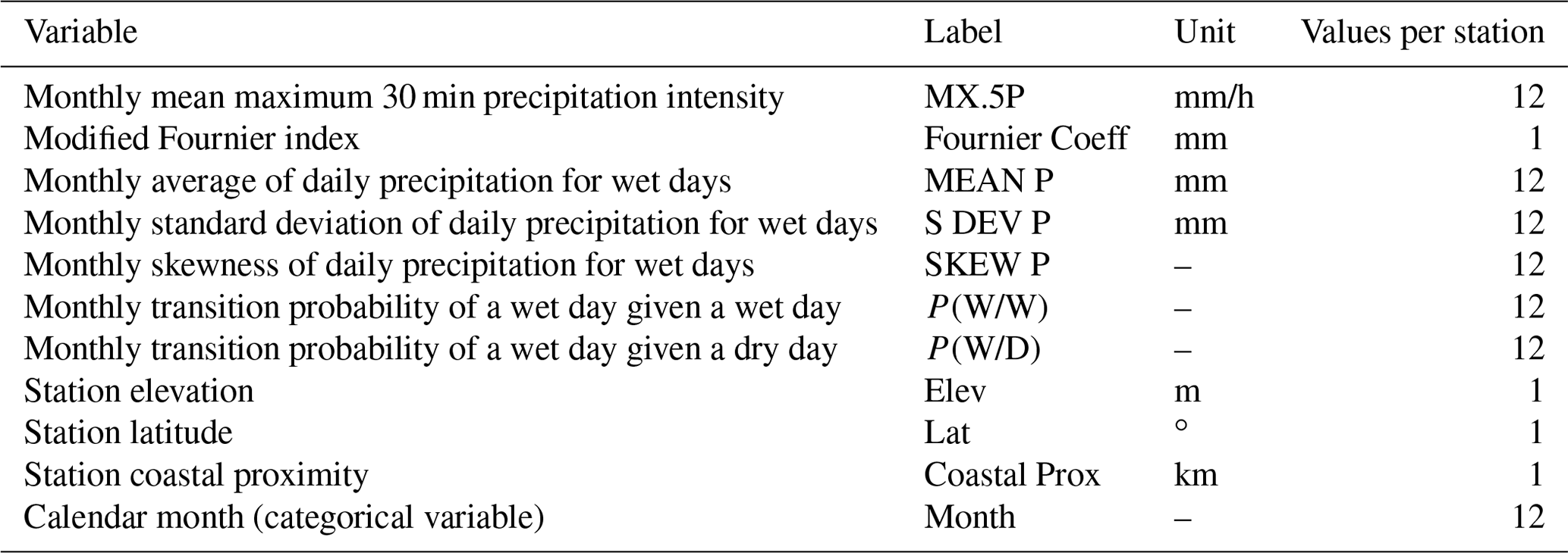
Table 3The 11 predictor variables for the gradient-boosting regression model used to temporally downscale MX.5P from GHCN-Daily data. Units were changed to metric for the purposes of the downscaling model.
2.3 Precipitation intensity
In soil erosion and runoff modeling, precipitation intensity is a critical factor (Pruski and Nearing, 2002; Nearing et al., 2005). The two parameters related to precipitation intensity, MX.5P and TimePk (refer to Table 2 for definitions), require data with high-frequency measurements such that hyetographs for a single precipitation event may be resolved. Since GHCN-Daily did not have adequate temporal resolution, MX.5P was estimated from the daily data using a temporal downscaling model, and TimePk was assumed to follow representative TimePk values for given Köppen–Geiger climate classifications. The development of these procedures is discussed in Fullhart et al. (2020b, 2021). High-resolution data needed for these procedures came from the Automated Surface Observing System (ASOS) maintained by NOAA with stations distributed across the United States and its territories (Doesken et al., 2002).
In CLIGEN, the MX.5P input parameter is used to parameterize statistical distributions of normalized peak intensity. The definition of MX.5P is as follows:
where k is the number of times (years) a record for a given month exists in the dataset, and maxI30 is the maximum 30 min intensity (mm h−1) for each monthly record (Yu, 2005). Since maximum 30 min intensity is most accurately determined from data with as high frequency of measurement as possible, deriving values from data with lower resolutions results in underestimation bias, therefore necessitating use of the temporal downscaling model for MX.5P. The downscaling model took GHCN-Daily data to estimate the MX.5P value that would be expected if derived from the 1 min data. The downscaling model is a machine learning regression using gradient boosting trained with 609 ASOS stations (Fullhart et al., 2020b). The model requires 11 predictor variables shown in Table 3, which are statistics that may be determined from daily data and geographic information, some of which are already CLIGEN inputs. While MX.5P from 1 min resolution was estimated by the model, the predictor variable with the single most predictive power was MX.5P derived from daily data, which was calculated based on an assumption that intensity was constant for the duration of daily intervals (and was therefore grossly underestimated). MEAN P and S DEV P were also important predictors. The MX.5P values estimated by the model were found to have an RMSE of 0.148 in. (3.76 mm) (Fullhart et al., 2020b).
The second intensity parameter, TimePk, represents values at 12 equal intervals along the cumulative distribution function (CDF) of normalized time-to-peak intensity for events recorded at a given station (TimePk is the only input parameter that does not represent monthly values, though there are 12 values per station, each representing quantiles of the CDF). For a given TimePk interval, the definition is as follows:
where TimePk(i) is the TimePk value at interval i, tp is time-to-peak intensity normalized to the event duration, is the number of events where tp , and Ntot is the total number of events. Interval, i, ranges between and and varies by increments of (Yu, 2005). Events were separated by >=6 h of no precipitation.
In Fullhart et al. (2021), it was shown that using climate-average TimePk values for the Köppen–Geiger climate classification of a given station resulted in <10 % error relative to true TimePk values, suggesting little variation in TimePk within climate classifications. In this previous study, a different weather station network was used – the U.S. Climate Reference Network (USCRN) at 5 min resolution (Diamond et al., 2013). For the new dataset of CLIGEN inputs, the analysis was repeated for the climate classifications represented by the 1 min ASOS network, though in some cases, climate classifications exclusive to the USCRN were used. Table A1 shows the assumed TimePk values for each climate classification. Of the 30 highest-order climate classifications, 19 were represented by ASOS and USCRN. The remaining 11 classifications were assumed to be the averages of the other TimePk values within respective first-order groups (of which there are five, where A is tropical, B is arid, C is temperate, D is cold, and E is polar). As such, the climate classification of each station was used to index the assumed TimePk values used in the CLIGEN input files. The climate classification of each station was determined based on the Köppen–Geiger climate map of Beck et al. (2018) representing the 1980–2016 time period at 0.083∘ resolution.
2.4 Temperature
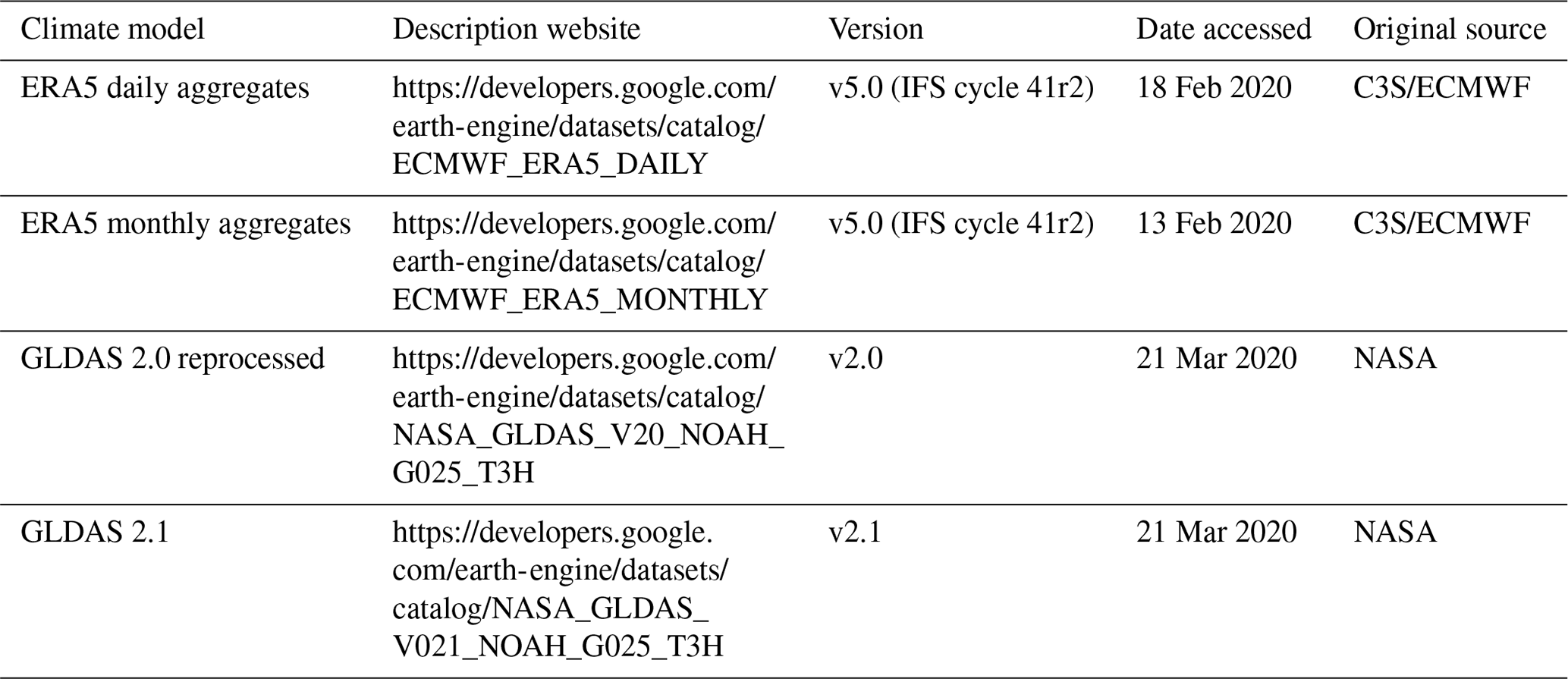
The five temperature-related parameters, TMAX AV, TMIN AV, SD TMAX, SD TMIN, and DEW PT (refer to Table 2 for definitions), have straightforward calculations. However, the required data were only available for a subset of GHCN-Daily stations. To avoid limiting the analysis to this subset of stations, these data were instead derived from the model outputs of the ERA5 global meteorological/climate analysis (“ECMWF ReAnalysis”, with ERA5 being the fifth major global reanalysis). The ERA5 analysis was created by The European Centre for Medium-Range Weather Forecasts and the Copernicus Climate Change Service (Albergel et al., 2018; Hersbach et al., 2020). Google Earth Engine was used to download maximum and minimum temperatures at daily resolution and average dew point temperatures at monthly resolution from a grid with 0.25∘ × 0.25∘ spatial resolution (see Table A3 for more information). Values obtained from the grid were unchanged, without any weighting based on proximity to neighboring cells or other forms of interpolation. The monthly dew point temperature was a convenient aggregation of data equivalent to the DEW PT CLIGEN parameter, while daily resolution was needed for the remaining CLIGEN temperature parameters to determine both the average and standard deviation of daily max–min temperatures. Use of the ERA5 model also allowed continuous time series to be obtained without gaps for the 30-, 20-, and 10-year datasets (from 1990 through 2019, 2000 through 2019, and 2010 through 2019, respectively).
2.5 Solar radiation
Incoming shortwave radiation is represented in CLIGEN by the SOL.RAD and SD RAD parameters (refer to Table 2 for definitions) that require solar radiation with units of langley/d where 1 langley = 41 840 J/m2. These parameters were calculated with relatively high-frequency (3 h) estimates that captured daily and day-to-day variability of radiation taken from the Global Land Data Assimilation System (GLDAS) model produced by NASA (Fang et al., 2009) at 0.25∘ × 0.25∘ resolution (see Table A3 for more information). The outputs of the reprocessed GLDAS 2.0 and GLDAS 2.1 versions were used and downloaded from Google Earth Engine (again, no weighting of values was done based on proximity to neighboring cells). The most recent data available were used to create continuous time series with temporal ranges being the same as those for the temperature parameters. For an individual day, incoming solar radiation was modeled by fitting a Gaussian curve through the 3 h time-averaged data points. Doing this avoided underestimation caused by time-averaging, which would have occurred by considering the 3 h data points alone. Also, if the 3 h intervals did not coincide with the time of peak intensity, comparison to ground observations from AmeriFlux data (discussed more later) showed that the Gaussian curve tended to better approximate peak radiation than the greatest 3 h data point.
A number of stations that existed on coasts or on small islands, particularly in the Pacific Ocean, did not have solar radiation data coverage for their locations because the GLDAS product covers only locations beyond a certain coastal proximity. In total, 390 stations had this problem. For these stations, data from the nearest station with existing data were used. A total of 300 of the stations with missing data were within 100 km of a station with data. Some proximities, however, were much further, with islands in the South Pacific being examples. Similarly, some locations in the existing US CLIGEN input dataset used for validation created by Srivastava et al. (2019) did not have observed solar radiation, and their parameter values were taken from the nearest station with available data, which in some cases were at considerable distances, potentially leading to poor validation in Sect. 3.
To ensure locations are matched for validation, a separate validation from that of Sect. 3 was done for solar radiation parameters. In this, GLDAS output was compared to 10 ground-based AmeriFlux stations that monitor ecosystem fluxes including solar radiation (Hargrove et al., 2003). The AmeriFlux network has stations distributed across the North and South American continents, and the 10 stations were selected from a range of latitudes and climates as a representation of global variability. From these stations, a single year was selected that had the fewest data gaps. Comparison to corresponding GLDAS outputs showed reasonable agreement with an RMSE of 36.6 langley/d and with GLDAS being overestimated by <1 % for monthly values of SOL.RAD. Error was more evident for SD RAD, suggesting that GLDAS was not optimum for capturing the day-to-day variability of radiation. The RMSE for SD RAD was 38.6 langley/d with GLDAS being underestimated by 24.1 %.
2.6 Wind
Very few applications of CLIGEN have used wind data in the past, perhaps the only one being the blowing snow component in WEPP (Nicks et al., 1989). CLIGEN inputs require high-frequency measurement of wind speed (m/s) and azimuthal wind direction. This includes mean, standard deviation, and skewness of daily wind speed on a monthly basis, and determinations of the average daily percentage of time with wind directions coming from the four cardinal directions, four intercardinal directions, and the eight sub-divisions of these (e.g., NNE, ENE) on a monthly basis. However, wind data were not obtainable for the locations corresponding to the GHCN-Daily stations with the level of detail needed for creating CLIGEN input files. The solution to this was to use the “International Conversion Programs” tool (availability given in Sect. 4), which takes the known daily precipitation accumulation and temperature parameters from an international station of interest and finds the existing station in the US CLIGEN dataset with the most similar climate, allowing its wind parameters to be used (and other remaining parameters, if needed). Information regarding the locations from where wind parameters were taken from is given at the bottom of each input file.
Table 4Summary of the validation of parameters to the 2015 US CLIGEN dataset created by Srivastava et al. (2019).
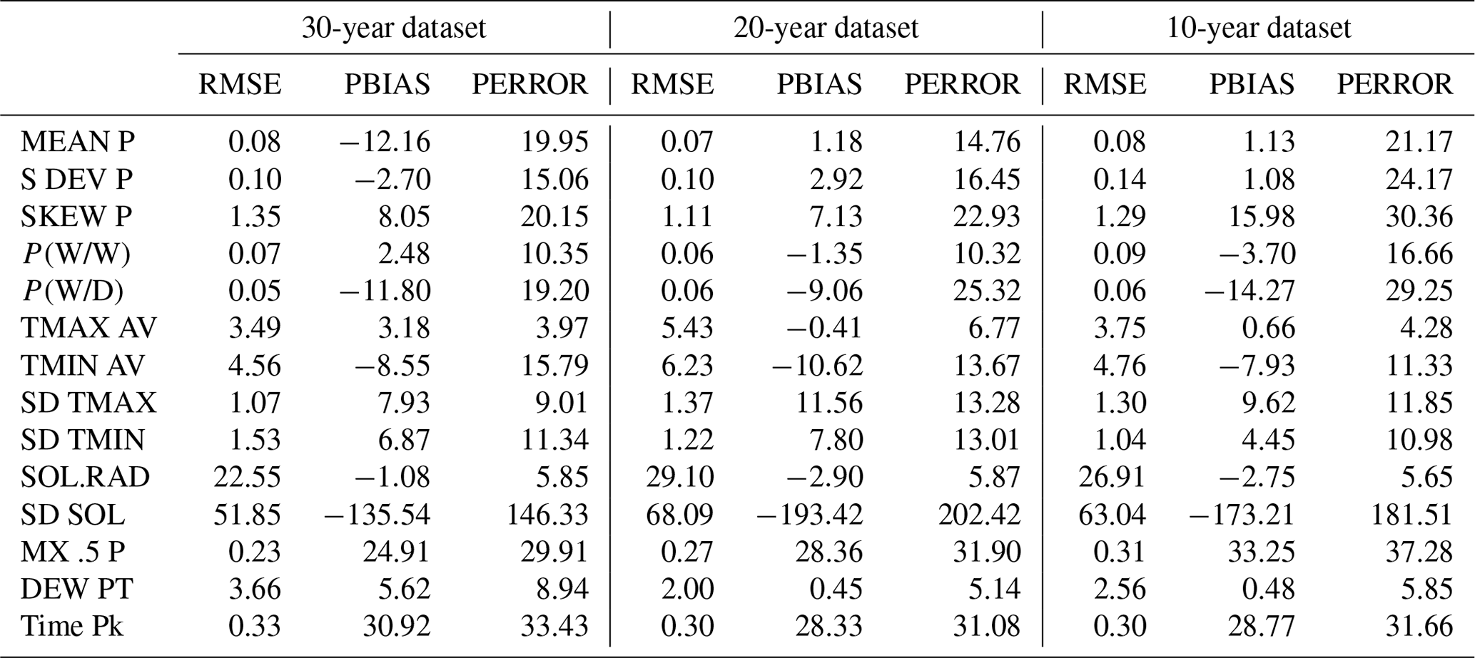
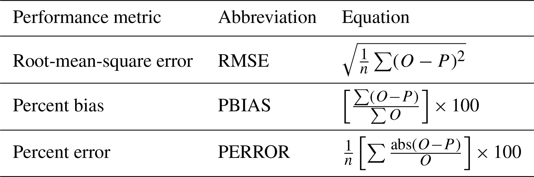
Each parameter except for the wind parameters was compared to an existing dataset for the US and its territories created in 2015 using NOAA NCDC DSI-3260 data at 15 min resolution and consisting of 40-year records for 2648 stations (Srivastava et al., 2019). This limited the validation to only stations for the US, and from those, only the new stations within 10 km of an existing CLIGEN station were accepted. This resulted in the validation of 61 stations for the 30-year dataset, 53 stations for the 20-year dataset, and 204 stations for the 10-year dataset. For each of the validated parameters, RMSE, percent bias, and percent error were determined, where it was assumed that values from the existing US dataset were the true values (performance metric definitions are given in Table A2). A summary of the validation is seen in Table 4. Inconsistencies between the two datasets were attributed to differences of data sources, differences in temporal resolution of data used, differences in record lengths, and whether data were interpolated or taken from nearby stations.
Overall, reasonable agreement was found, with PERROR being below 20 % for the majority of parameters. As expected, record length is a factor in the comparison to the 40-year US dataset. Percent error increased slightly on average (∼5 %) with decreasing record length, going from the 30- to 10-year datasets. Though a small increase, this difference likely reflected the potential for capturing short-term climate dynamics by the 20- and 10-year datasets. For the five parameters related to daily accumulation, the parameter with the highest error was SKEW P, with error up to 30 %. The sign of PBIAS for SKEW P was consistently positive, suggesting that the GHCN-Daily data showed less skewness towards high daily accumulation.
Error was also considerable for the two parameters related to precipitation intensity, MX.5P and TimePk. The discrepancies were due to multiple issues including the fact that the DSI-3260 dataset uses 15 min resolution compared to the 1 min resolution that the MX.5P downscaling model and TimePk distributions were based on. As mentioned, the downscaling model was previously shown to produce an average error of 0.148 in. (3.76 mm) (Fullhart et al., 2020b). In the comparison to the DSI-3260 dataset, downscaled MX.5P values resulted in discrepancy of up to 37 % error for MX.5P. Interval values for TimePk distributions were generally smaller in magnitude and approached unity later in the distribution, meaning that the peak intensity of storms generally happened later in their duration than in the DSI-3260 data. This may be expected given the relatively coarse 15 min resolution of DSI-3260, and particularly when considering shorter storms, such as convective storms, the apparent peak intensity may have considerable uncertainty.
Temperature parameters were generally in agreement with no consistent estimation bias, except for DEW PT, which was slightly underestimated on average by up to 6 %. Errors for SOL.RAD were up to 6 %, with a slight overestimation bias of up to 3 %. While SOL.RAD was in good agreement, SD SOL indicated up to 193 % more day-to-day variability of solar radiation. The GLDAS data for solar radiation generally agreed better with the variability of the AmeriFlux network that was discussed in Sect. 2.5, with GLDAS showing 24 % less variability than AmeriFlux. Given the reasonable agreement between GLDAS and AmeriFlux, and good agreement of SOL.RAD with the DSI-3260 data, the substantial underestimation bias of SD SOL may be the result of errors in the existing US inputs.
While the US represents a wide range of climate types, limitation of the validation to only the US is a hinderance to quality assurance of the new dataset. However, each of the source data have their own quality assurances prior to going to product. Particularly for the ERA5 and GLDAS global products, biases are documented and are known to happen on regional and continental spatial scales and may relate to extremes in temperature, moisture, geographic location, etc. (Zhou et al., 2013; Ji et al., 2015; Urraca et al., 2018; Wang et al., 2019). Therefore, the uncertainty of each CLIGEN parameter also depends on the particular source data.
The new international CLIGEN input dataset is available at the National Agriculture Library Online Repository – Ag Data Commons – at https://data.nal.usda.gov/dataset/international-climate-benchmarks-and-input-parameters-stochastic-weather-generator-cligen (last access: 11 February 2021) (Fullhart et al., 2020a; DOI: https://doi.org/10.15482/USDA.ADC/1518706) and is separated into three datasets according to 30-, 20-, and 10-year record lengths. To run the CLIGEN inputs, CLIGEN may be downloaded at https://www.ars.usda.gov/midwest-area/west-lafayette-in/national-soil-erosion-research/docs/wepp/cligen/ (last access: 11 February 2021). Additional resources and materials are available at this website including the “International Conversion Programs” tool. The international CLIGEN dataset will also be added to the web interface for running the hillslope-scale erosion and runoff model, RHEM, available at https://apps.tucson.ars.ag.gov/rhem/ (last access: 11 February 2021). The station of interest will be selectable in the input parameter panel under “Climate Station” and under “International”.
Validation of CLIGEN inputs in the new international dataset showed reasonable agreement with parameter values for existing US CLIGEN inputs. The 30-, 20-, and 10-year datasets are generally in close agreement, and in some cases, the methods used to create this dataset may offer an improvement over existing CLIGEN input files. However, issues arise due to the assumptions that were taken for addressing pervasive data gaps in NOAA-GHCN records. Validation of the climate benchmarks by comparison to other records is complicated by use of discontinuous time series, and uncertainty is higher in places with non-stationary climates or long-term cycles.
The new dataset of CLIGEN inputs allows the CLIGEN weather generator to be more readily applied to its various applications. The input files also serve to represent climate benchmarks for a selection of variables that are generally unobtainable from a single source. The coverage of stations is particularly dense in Europe, Australia, and North America and offers the potential to improve the spatial analysis of processes in different fields that require climate records. For a number of CLIGEN's applications, the production of climate data is a secondary concern but is often a labor-intensive task. The use of this dataset may allow researchers to put more effort and resources towards their primary study or area of focus without needing to address the production of climate inputs.
Table A1TimePk distribution interval values for global Köppen–Geiger climate classifications.
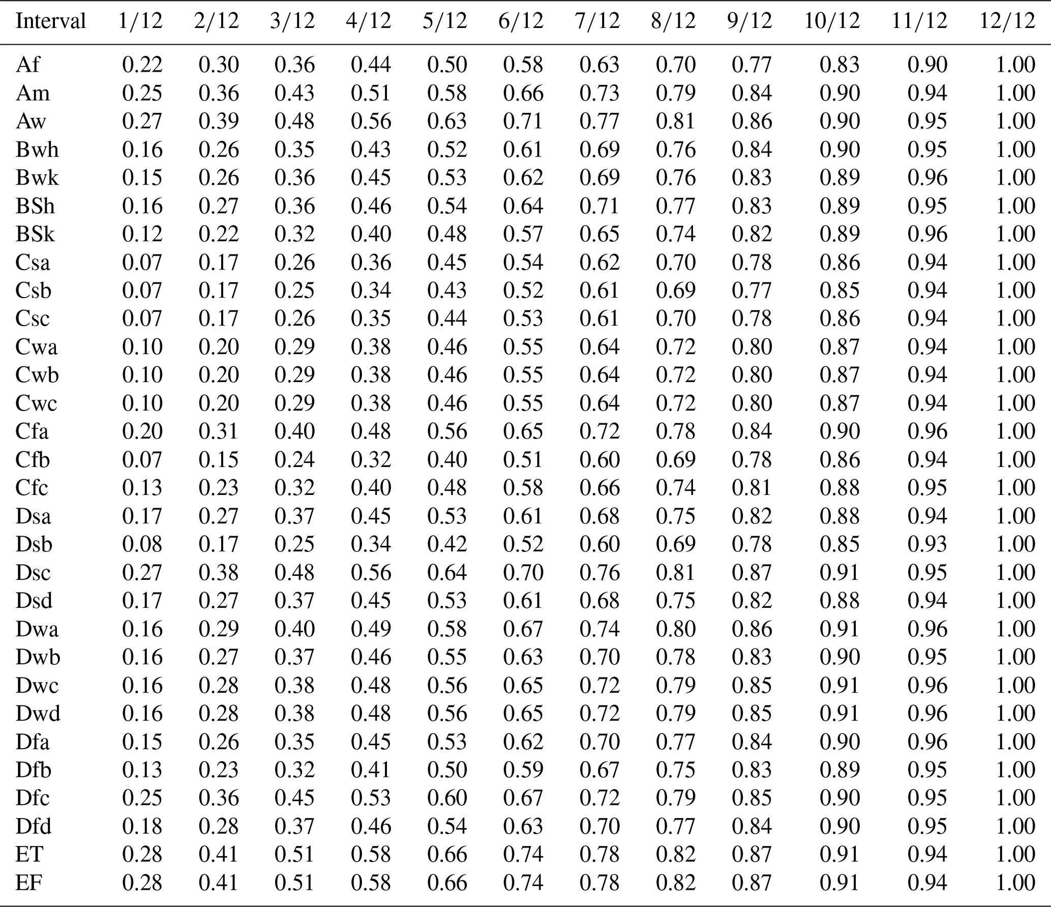
Table A2Statistical measures of performance. Observed (O) and predicted (P) values are compared by each metric.
ATF calculated input parameters, GA provided expertise on data management and integration with the RHEM web interface, MAN and MAW gave their expertise on project guidance, and all authors were involved in writing the manuscript.
The authors declare that they have no conflict of interest.
The authors wish to express their appreciation for everyone involved in creating and maintaining the various climate networks that were used. Funding for this project was given through the Agricultural Research Service Headquarters Grant and the Southwest Watershed Research Center.
This paper was edited by David Carlson and reviewed by two anonymous referees.
Albergel, C., Dutra, E., Munier, S., Calvet, J.-C., Munoz-Sabater, J., de Rosnay, P., and Balsamo, G.: ERA-5 and ERA-Interim driven ISBA land surface model simulations: which one performs better?, Hydrol. Earth Syst. Sci., 22, 3515–3532, https://doi.org/10.5194/hess-22-3515-2018, 2018.
Baffaut, C., Nearing, M. A., and Nicks, A. D.: Impact of CLIGEN parameters on WEPP-predicted average annual soil loss, T. ASAE, 39, 447–457, 1996.
Beck, H. E., Zimmermann, N. E., McVicar, T. R., Vergopolan, N., Berg, A., and Wood, E. F.: Present and future Köppen-Geiger climate classification maps at 1-km resolution, Sci. Data, 5, 180214, https://doi.org/10.1038/sdata.2018.214, 2018.
Bojinski, S., Verstraete, M., Peterson, T. C., Richter, C., Simmons, A., and Zemp, M.: The concept of essential climate variables in support of climate research, applications, and policy, B. Am. Meteorol. Soc., 95, 1431–1443, https://doi.org/10.1175/BAMS-D-13-00047.1, 2014.
Diamond, H. J., Karl, T. R., Palecki, M. A., Baker, C. B., Bell, J. E., Leeper, R. D., Easterling, D. R., Lawrimore, J. H., Meyers, T. P., Helfert, M. R., Goodge, G., and Thorne, P. W.: US Climate Reference Network after one decade of operations: Status and assessment, B. Am. Meteorol. Soc, 94, 485–498, https://doi.org/10.1175/BAMS-D-12-00170.1, 2013.
Doesken, N. J., McKee, T. B., and Davey, C.: Climate data continuity – what have we learned from the ASOS automated surface observing system, Proc. 13th Conf. App. Clim., Portland, Oregon, 13–16 May, 2.7, 2002.
Durre, I., Menne, M. J., Gleason, B. E., Houston, T. G., and Vose, R. S.: Comprehensive automated quality assurance of daily surface observations, J. App;. Meteorol. Clim., 49, 1615–1633, https://doi.org/10.1175/2010JAMC2375.1, 2010.
Fang, H., Beaudoing, H. K., Teng,W. L., and Vollmer, B. E.: Global Land Data Assimilation System (GLDAS) products, services and application from NASA hydrology data and information services center (HDISC), ASPRS Ann. Conf., Baltimore, Maryland, 8–13 March, 1–9, 2009.
Fullhart, A. T., Nearing, M. A., Armendariz, G., and Weltz, M. A.: International climate benchmarks and input parameters for a stochastic weather generator, CLIGEN (dataset), Ag Data Commons, https://doi.org/10.15482/USDA.ADC/1518706, 2020a.
Fullhart, A. T., Nearing, M. A., McGehee, R. P., and Weltz, M. A.: Temporally downscaling a precipitation intensity factor for soil erosion modeling using the NOAA-ASOS weather station network, Catena, 194, 104709, https://doi.org/10.1016/j.catena.2020.104709, 2020b.
Fullhart, A. T., Nearing, M. A., and Weltz, M. A.: Temporally downscaling precipitation intensity factors for Köppen climate regions in the U.S., J. So. Wat. Con., 76, 39–51, https://doi.org/10.2489/jswc.2021.00156, 2021.
Hargrove, W. W., Hoffman, F. M., and Law, B. E.: New analysis reveals representativeness of the AmeriFlux network, EOS T. Am. Geophys. Un., 84, 529–535, https://doi.org/10.1029/2003EO480001, 2003.
Hersbach, H., Bell, B., Berrisford, P., Hirahara, S., Horányi, A., Muñoz-Sabater, J., Nicolas, J., Peubey, C., Radu, R., Schepers, D., Simmons, A., Soci, C., Abdalla, S., Abellan, X., Balsamo, G., Bechtold, P., Biavati, G., Bidlot, J., Bonavita, M., De Chiara, G., Dahlgren, P., Dee, D., Diamantakis, M., Dragani, R., Flemming, J., Forbes, R., Fuentes, M., Geer, A., Haimberger, L., Healy, S., Hogan, R. J., Hólm, E., Janisková, M., Keeley, S., Laloyaux, P., Lopez, P., Lupu, C., Radnoti, G., de Rosnay, P., Rozum, I., Vamborg, F., Villaume, S., and Thépaut, J.: The ERA5 global reanalysis, Q. J. Roy. Meteor. Soc., 730, 1999–2049, https://doi.org/10.1002/qj.3803, 2020.
Hollmann, R., Merchant, C. J., Saunders, R., Downy, C., Buchwitz, M., Cazenave, A., Chuvieco, E., Defourny, P., de Leeuw, G., Forsberg, R., Holzer-Popp, T., Paul, F., Sandven, S., Sathyendranath, S., van Roozendael, M., and Wagner, W.: The ESA climate change initiative: Satellite data records for essential climate variables, B.. Am. Meteorol. Soc., 94, 1541–1552, https://doi.org/10.1175/BAMS-D-11-00254.1, 2013.
IPCC: Climate Change 2013: The Physical Science Basis, Summary for Policymakers. Contribution of Working Group I to the Fifth Assessment Report of the Intergovernmental Panel on Climate Change, Cambridge University Press, Cambridge, United Kingdom and New York, NY, USA, 2013.
Ji, L., Senay, G. B., and Verdin, J. P.: Evaluation of the Global Land Data Assimilation System (GLDAS) air temperature data products, J. Hydrometeorol., 16, 2463–2480, https://doi.org/10.1175/JHM-D-14-0230.1, 2015.
Kinnell, P. I. A.: CLIGEN as a weather generator for RUSLE2, Catena, 172, 877–880, https://doi.org/10.1016/j.catena.2018.09.016, 2019.
Lobo, G. P., Frankenberger, J. R., Flanagan, D. C., and Bonilla, C. A.: Evaluation and improvement of the CLIGEN model for storm and rainfall erosivity generation in Central Chile, Catena, 127, 206–213, https://doi.org/10.1016/j.catena.2015.01.002, 2015.
Mehan, S., Guo, T., Gitau, M. W., and Flanagan, D. C.: Comparative study of different stochastic weather generators for long-term climate data simulation, Climate, 5, 26, https://doi.org/10.3390/cli5020026, 2017.
Menne, M. J., Durre, I., Vose, R. S., Gleason, B. E., and Houston, T. G.: An overview of the Global Historical Climatology Network-Daily Database, J. Atmos. Ocean. Tech., 29, 897–910, https://doi.org/10.1175/JTECH-D-11-00103.1, 2012.
Nearing, M. A., Jetten, V., Baffaut, C., Cerdan, O., Couturier, A., Hernandez, M., Le Bissonnais, Y., Nichols, M. H., Nunes, J. P., Renschler, C. S., Souchere, V., and van Oost, K.: Modeling response of soil erosion and runoff to changes in precipitation and cover, Catena, 61, 131–154, https://doi.org/10.1016/j.catena.2005.03.007, 2005.
Nicks, A. D., Lane, L. J., Nearing, M. A., and Stone, J. J.: WEPP hillslope profile erosion model user summary, USDA – Water Erosion Prediction Project: Hillslope Profile Model Documentation, NSERL Report, 2, 1989.
Panagos, P., Borrelli, P., Meusburger, K., Yu, B., Klik, A., Lim, K. J., and Sadeghi, S. H.: Global rainfall erosivity assessment based on high-temporal resolution rainfall records, Sci. Rep.-UK, 7, 1–12, https://doi.org/10.1038/s41598-017-04282-8, 2017.
Pruski, F. F. and Nearing, M. A.: Runoff and soil-loss responses to changes in precipitation: A computer simulation study, J. So. Wat. Con., 57, 7–16, 2002.
Srivastava, A., Flanagan, D. C., Frankenberger, J. R., and Engel, B. A.: Updated climate database and impacts on WEPP model predictions, J. So. Wat. Con., 74, 334–349, https://doi.org/10.2489/jswc.74.4.334, 2019.
Urraca, R., Huld, T., Gracia-Amillo, A., Martinez-de-Pison, F. J., Kaspar, F., and Sanz-Garcia, A.: Evaluation of global horizontal irradiance estimates from ERA5 and COSMO-REA6 reanalyses using ground and satellite-based data, Sol. En., 164, 339–354, https://doi.org/10.1016/j.solener.2018.02.059, 2018.
Vaghefi, P. and Yu, B.: Use of CLIGEN to simulate decreasing precipitation trends in the southwest of Western Australia, Trans. ASABE, 59, 49–61, https://doi.org/10.13031/trans.59.10829, 2016.
Vaghefi, P. and Yu, B.: Validation of CLIGEN parameter adjustment methods for Southeastern Australia and Southwestern Western Australia, J. Hydrometeorol., 18, 2011–2028, https://doi.org/10.1175/JHM-D-16-0237.1, 2017.
Wang, C., Graham, R. M., Wang, K., Gerland, S., and Granskog, M. A.: Comparison of ERA5 and ERA-Interim near-surface air temperature, snowfall and precipitation over Arctic sea ice: effects on sea ice thermodynamics and evolution, The Cryosphere, 13, 1661–1679, https://doi.org/10.5194/tc-13-1661-2019, 2019.
Wischmeier, W. H. and Smith, D. D.: Predicting rainfall erosion losses: A guide to conservation planning (Agricultural Handbook No. 537), Department of Agriculture, Science and Education Administration, Washington, D.C., 001-000-03903-2, 1978.
Yu, B.: Adjustment of CLIGEN parameters to generate precipitation change scenarios in southeastern Australia, Catena, 61, 196–209, https://doi.org/10.1016/j.catena.2005.03.004, 2005.
Zhang, X. C.: Generating correlative storm variables for CLIGEN using a distribution-free approach, T. ASAE, 48, 567–575, https://doi.org/10.13031/2013.18331, 2005.
Zhang, X. C. J.: Adjusting skewness and maximum 0.5 hour intensity in CLIGEN to improve extreme event and sub-daily intensity generation for assessing climate change impacts, Trans. ASABE, 56, 1703–1713, https://doi.org/10.13031/trans.56.10004, 2013.
Zhang, Y., Liu, B., Wang, Z., and Zhu, Q.: Evaluation of CLIGEN for storm generation on the semiarid Loess Plateau in China, Catena, 73, 1–9, https://doi.org/10.1016/j.catena.2007.08.001, 2008.
Zhou, X., Zhang, Y., Yang, Y., and Han, S.: Evaluation of anomalies in GLDAS-1996 dataset, Wat. Sci. Tech., 67, 1718–1727, https://doi.org/10.2166/wst.2013.043, 2013.