the Creative Commons Attribution 4.0 License.
the Creative Commons Attribution 4.0 License.
 | 20 Aug 2021
An integrated marine data collection for the German Bight – Part 1: Subaqueous geomorphology and surface sedimentology (1996–2016)
Peter Milbradt
Romina Ihde
Jennifer Valerius
Robert Hagen
Andreas Plüß
The German Bight located within the central North Sea is a hydro- and morphodynamically highly complex system of estuaries, barrier islands, and part of the world's largest coherent tidal flats, the Wadden Sea. To identify and understand challenges faced by coastal stakeholders, such as harbor operators or governmental agencies, to maintain waterways and employ numerical models for further analyses, it is imperative to have a consistent database for both bathymetry and surface sedimentology. Current commercial and public data products are insufficient in spatial and temporal resolution and coverage for recent analysis methods. Thus, this first part of a two-part publication series of the German joint project EasyGSH-DB describes annual bathymetric digital terrain models at a 10 m gridded resolution for the German North Sea coast and German Bight from 1996 to 2016 (Sievers et al., 2020a, https://doi.org/10.48437/02.2020.K2.7000.0001), as well as surface sedimentological models of discretized cumulative grain size distribution functions for 1996, 2006, and 2016 on 100 m grids (Sievers et al., 2020b, https://doi.org/10.48437/02.2020.K2.7000.0005). Furthermore, basic morphodynamic and sedimentological processing analyses, such as the estimation of, for example, bathymetric stability or surface maps of sedimentological parameters, are provided (Sievers et al., 2020a, b, see respective download links).
- Article
(10140 KB) - Full-text XML
- BibTeX
- EndNote


The German Bight and the adjacent central North Sea (Fig. 1) are highly complex systems of barrier islands, the world's largest coherent system of coastal tidal flats and multiple estuaries (Elias et al., 2012; Kabat et al., 2012; Benninghof and Winter, 2019). Recent research interest frequently focuses on the morpho- and hydrodynamic processes in this area, e.g., Elias et al. (2012), Zijl et al. (2013), Heyer and Schrottke (2015), Wang et al. (2015), and Benninghof and Winter (2019). For this, numerical models of various implementations require input parameters gained from, for example, bathymetric or sedimentological datasets to gain further insight and understand longer-term processes (Zijl et al., 2013; Arns et al., 2015; Wang et al., 2018; Rasquin et al., 2020) such as the sea level rise. Harbor operators for small- and large-scale maritime industry and tourism and other marine actors need to be able to identify, understand, and potentially counteract changes and developments to the coastline and estuaries and the surface sedimentology to maintain and operate within a profitable margin, as well as to be prepared for potential hazardous situations (Roeland and Piet, 1995; Kirichek et al., 2018; Wölfl et al., 2019; Kiricheck et al., 2020). Additionally, further applications that are not directly obvious are dependent on bathymetric information, such as search efforts in open-sea scenarios (Wölfl et al., 2019). It is thus vital to have a consistent set of high-resolution elevation and surface sediment information.
Currently available datasets which are highly volatile in spatial and temporal resolution and coverage are compiled in publicly accessible portals and services (Wölfl et al., 2019). Portals and services such as EMODnet Bathymetry (http://www.emodnet-bathymetry.eu, last access: 16 August 2021), GEBCO (http://www.gebco.net, last access: 16 August 2021), or ETOPO (http://www.ngdc.noaa.gov, last access: 16 August 2021) offer bathymetric datasets with spatial resolutions of 70 m to approximately 2 km, depending on the overall spatial coverage, yet in part there is no certain indication about important quality elements, such as currentness or timeliness and traceability or data source, of the utilized dataset. Surface sedimentological information of the central North Sea are coarse for applications in numerical models with spatial resolutions of approximately 2 to 13 km with predetermined classifications and analyses such as median grain diameter already performed and provided by, for example, Helmholtz Zentrum Geesthacht (https://www.hereon.de, last access: 16 August 2021), EMODnet Geology (http://www.emodnet-geology.eu, last access: 16 August 2021), or Wilson et al. (2018), which hinders the custom extraction of parameters such as sorting or skewness coefficients or grain size classes for use in numerical models. Portals for individual data publication, such as Pangaea (http://www.pangaea.de, last access: 16 August 2021), usually offer local datasets at a high resolution. However, a low overall coverage results in a decrease in larger-scale scientific value as region-specific availability and consistency issues with adjacent data exist. Apart from spatial resolution and coverage issues, temporal information is in part inconsistent or unavailable. For hydro- and morphodynamically highly dynamic regions such as the German North Sea coast, a specific date or time span of validity is essential to adequately analyze the occurring processes.
The German joint project AufMod began the process of alleviating these issues with both increased temporal and spatial coverage and resolution (Heyer and Schrottke, 2015). Bathymetric regular 50 m gridded digital terrain models (DTMs) were provided from 1982 to 2012 for the inner German Bight, as well as surface sedimentological information including full discretized cumulative grain size distribution (GSD) functions for individual further processing at a 250 m grid resolution (Milbradt et al., 2015). However, state-of-the-art modeling studies deploy horizontal grids and meshes for bathymetry and sedimentology that require an even higher resolution than AufMod's initial steps (Zijl et al., 2013; Kösters and Winter, 2014; Hagen et al., 2020; Rasquin et al., 2020; Hagen et al., 2021). With AufMod ending in 2012, the data coverage is outdated.
This paper, as part one of a two-part publication, introduces an integrated data collection created in the German project EasyGSH-DB, which includes geomorphological and surface sedimentological products and analyses at a higher temporal and spatial resolution than previous products: 21 annual bathymetric terrain models spanning 1996 to 2016 as a 10 m regular grid and 3 surface sediment models of GSD functions valid for 1996, 2006, and 2016 on a 100 m grid are presented for the German Bight (Fig. 1). Additionally, the larger German Exclusive Economic Zone (EEZ) is covered in a 100 m bathymetric and 250 m surface sedimentological grid of continuous GSD functions. Additionally, basic further processing steps, such as the generation of elevation isobaths, bathymetric analyses, and sedimentological maps and parameters, are provided as well.
Part two of this publication (Hagen et al., 2021) displays hydrodynamic numerical modeling results based on the base data presented hereafter. All data products are available to download for free, if applicable, provided with additional metadata for quality and usability assessment.
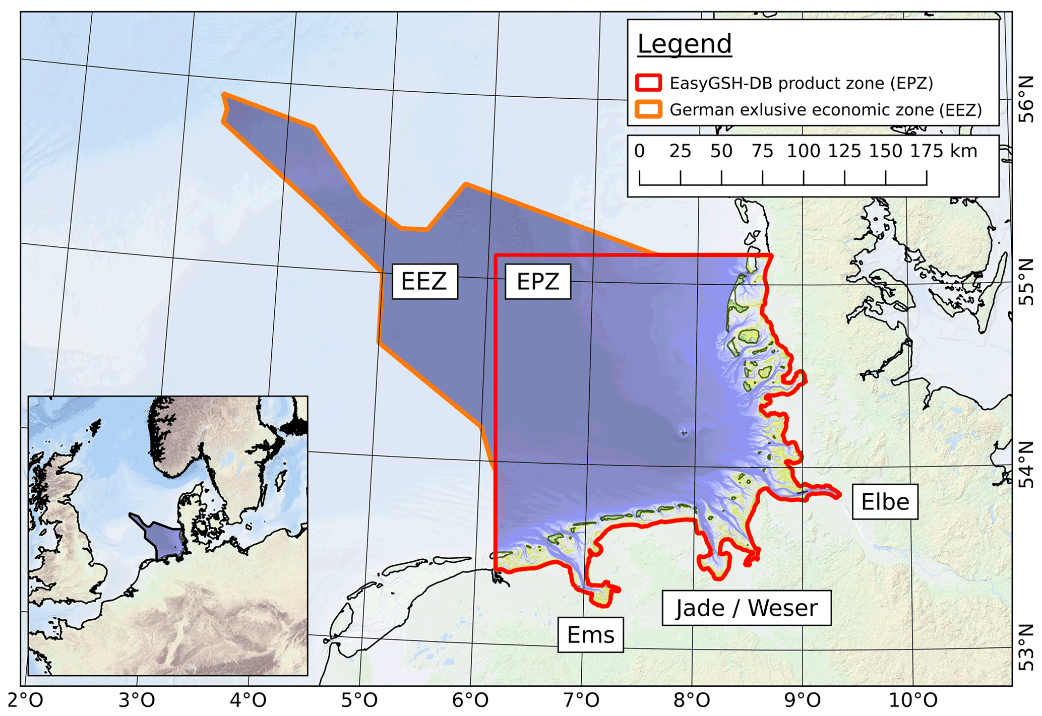
Figure 1Spatial extent of the German Bight with EasyGSH-DB's product zone (EPZ) and larger German Exclusive Economic Zone (EEZ) within the North Sea with a bathymetric model of 1996. Positions of major estuaries given for reference.

Figure 2Spatial extent of FSM database: (a) overlapping bathymetric datasets and (b) surface sedimentological datasets represented by continuous GSD functions.
Usually, the only way to obtain data valid for a specific date is to measure it at that specific point in time. Studies to undertake surveys at a very high, quasi-continuous temporal resolution alleviate this issue; they are, however, generally very small scale or on singular transects (Gallagher et al., 1998; Moulton et al., 2014). Concepts to temporally interpolate hydrographic and bathymetric information between fewer temporal sample points to reduce time and costs of such studies are well known (Moulton et al., 2014; Kuusela et al., 2018; Genchi et al., 2020), yet they still focus on singular series of samples of an isolated area. Missing synoptic analysis bringing together multiple surveys of such varying types and resolutions from different points in time and space classify most of these datasets as the previously mentioned highly regionalized individually published information. As digital terrain models (DTMs) today already aggregate data and employ spatial interpolation to create high coverage information, the next step is combining the spatial and temporal interpolation of multiple datasets to create not only a spatially but also temporally continuous model space for numerous applications.
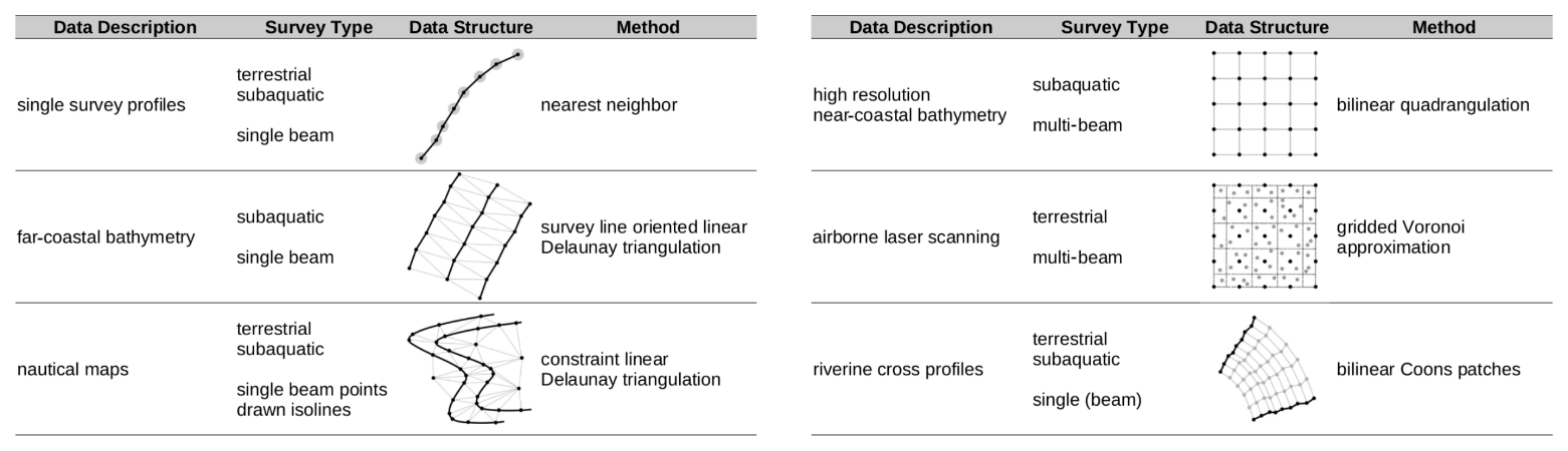
Figure 3Overview of the most common approximation and interpolation methods used for datasets of the FSM.

Figure 4Concept of spatiotemporal interpolation of bathymetric information.
2.1 Introduction to the Functional Seabed Model
The Functional Seabed Model is a holistic data-based hindcast simulation model (Milbradt et al., 2015) and was first utilized at a larger scale in the joint project AufMod (Heyer and Schrottke, 2015) to provide consistent DTMs and base data for numerical modeling and morphodynamic analyses from multiple datasets originating from separate surveys for user-defined spatial and temporal extent and validity.
In its current form, input data and thus spatial and temporal range cover primarily Germany, the southern and central North Sea, and the British Isles from the early 1950s until today. Its database contains approximately 127 000 elevation datasets with 115 billion single data points (Fig. 2a) and approximately 95 000 surface sediment samples represented by continuous grain size distribution (GSD) functions (Fig. 2b) to meet the requirements of advanced model systems as described in part two of this publication (Hagen et al., 2021). Approximately 45 000 surface sediment samples are located within the EEZ. For the highest attainable transparency of provenance of our products, each individual bathymetric and sedimentological dataset has metadata attached, which include among others sample title, source organization, and survey time as either an isolated instance or a temporal span.
Both bathymetric and surface sedimentological surveys create information at isolated points; thus interpolation and approximation methods are applied to create spatially continuous products for specific points in time. As surveys have varying purposes, they are undertaken as various survey types, and as a consequence, the structure of the initial processed dataset is highly variable as well. Consequently, the anticipated quality of spatial representation is highly dependent on the applied approximation or interpolation method itself. While linear interpolation may be sufficient in high-density surveys, they might not be adequate in other cases. This is where the FSM's ability to connect geometric datasets to metadata is of utmost importance. The aforementioned metadata information contains not only trivial entries such as the descriptive attributes but also information about the method that is to be utilized for the spatial interpolation of the specific dataset in question, including parameters such as search radii and required point counts. A small, non-exhaustive example of this survey-type-dependent approximation and interpolation definition defined for and utilized in the FSM is displayed in Fig. 3.
2.2 Spatiotemporal interpolation and approximation of bathymetric datasets
Spatial interpolation or approximation of bathymetric datasets in the FSM follows the well-known and fundamental concept of the linear combination of a weighting factor from a so-called base function and the data point elevation information. The base function is generally dependent on the spatial position of the data point and commonly produces weighting factors based on distances between data points and points to be interpolated or approximated. Both interpolation and approximation follow therefore Eq. (1), where is the interpolated or approximated elevation at a position x, is a weighting factor for point pi, which commonly returns 1 at point pi and 0 for all other points pk with i≠k, zi=z(pi) is the elevation of sample point pi, and n is the number of all data points within the dataset.
While both approximation and interpolation methods rely on the same core concept, only interpolation algorithms, as a special case of approximation, reliably reflect the original data point information at its position. Approximation methods do not need to fulfill this requirement. Regardless of the explicit implementation of the method itself, it is imperative to note that both interpolated and approximated values that do not coincide with the actual data points are estimations. Survey types and consequently interpolation or approximation methods (see Fig. 3) define the base functions to be used.
Temporal interpolation between two data points in time at the same spatial position is equivalent to spatial interpolation but instead utilizes not spatial but temporal distances as parameters for the base functions. It is necessary to employ temporal interpolation as surveys rarely take place at the desired point in time, and even if by coincidence they do regionally, on a larger scale they are not reasonably to be expected to have consistent coverage. Due to the generally high density of regional bathymetric surveys spatially and temporally, linear temporal interpolation (see Eq. 1) between the closest older and younger datasets with regard to the point in time and space is determined to be sufficient and subsequently used in the FSM. More advanced temporal interpolation approaches such as spline interpolations over all present datasets at a single point in space have been evaluated but were due to their extraordinarily high computation time paired with very little benefit in terms of quality of the modeled elevation disregarded for large-scale DTMs such as presented here.
Combining both spatial and temporal approaches yields the FSM's first and foremost defining quality: the spatiotemporal interpolation. Spatiotemporal interpolation of bathymetric datasets gives the ability to derive an elevation value and consequently DTMs at any given point in space and time within the FSM's model boundaries (see Fig. 4).
This combination is depicted in Eq. (2), where is the approximated or interpolated value at a position x at a time t, φi(t) is a weighting factor based on the point in time t of dataset i, which commonly returns 1 at time ti of dataset i and 0 for all tk with i≠k, is the interpolated or approximated value at a position x within dataset i (see Eq. 1), and n is the number of datasets used.
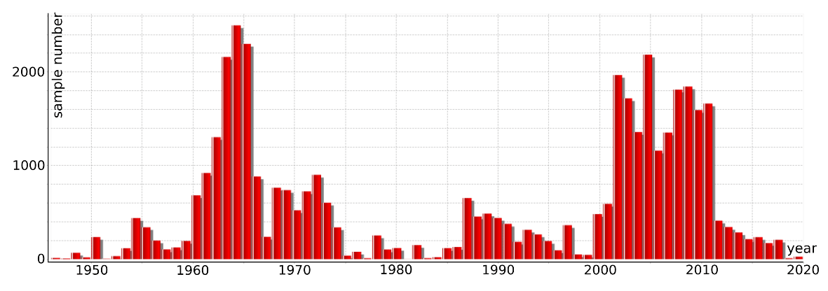
Figure 5Temporal distribution of approximately 45 000 surface sediment samples within the EEZ.
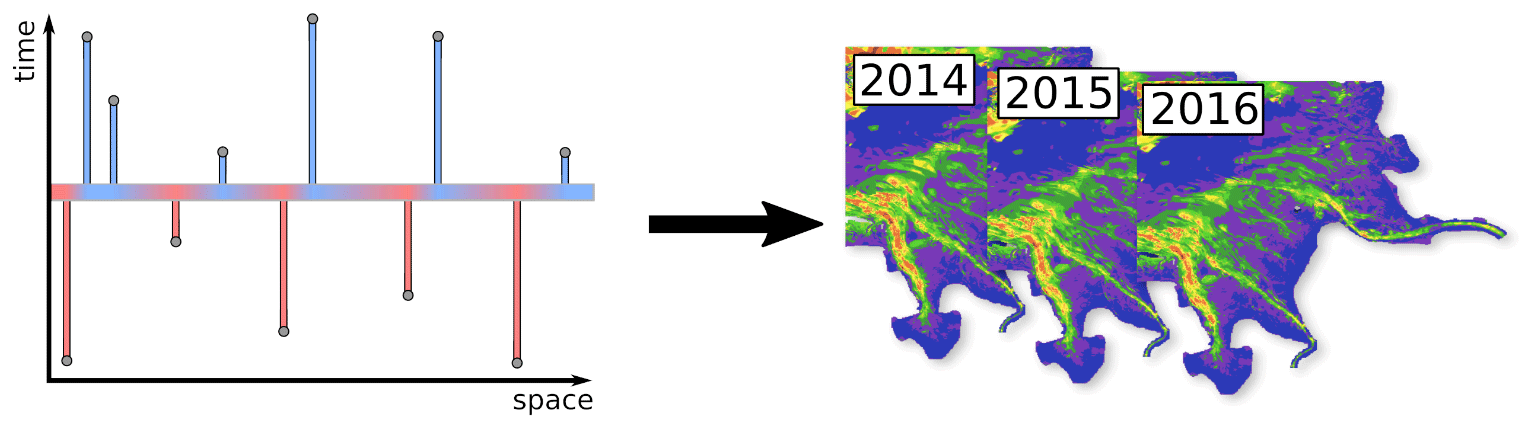
Figure 6Concept of spatiotemporal interpolation of surface sedimentological information.
2.3 Spatiotemporal interpolation and approximation of surface sedimentological datasets
Spatiotemporal interpolation of surface sedimentological datasets is met with additional obstacles compared to bathymetric information. Both the temporal and spatial density of surface sediment datasets, which are comprised of single sediment samples with single GSD functions, is much lower. Figure 5 displays the temporal distribution of the approximately 45 000 surface sediment samples within the EEZ (see Fig. 2b).
Apart from being highly variable, even in one of the years with the most samples taken, 1963, one sample represents on average approximately 5.7 km2 in the near-coastal environment, which is insufficient. Utilizing all samples regardless of their respective dates, however, would provide approximately one sample in 0.5 km2 for the highly dynamic near-coastal environment, which is in combination with the on average higher spatial density of samples in more active regions acceptable. As multiple samples at the same position are virtually non-existent, temporal interpolation as described before cannot be applied. Thus, an extrapolation approach was developed that relies on the parametrization of the cumulative GSD function into median grain size, sorting, and skewness coefficients based on Folk (1980) and an ordinary differential equation as an initial value problem. Equation (3) displays the solution as a time-dependent change of median grain size d50 for a point in time t, where λ(zb(t)) is a parametrization of depth fuzziness, which reduces the influence of elevation changes with greater depths due to measurement uncertainty, n(t) is the time-dependent relative surface porosity (see Sect. 2.4), is the stepwise sedimentation or erosion rate as derived from all bathymetric datasets at the sample position as a time series, σ0 is the initial approximated sorting of the surrounding sediment samples, and and are the logistic boundaries of d50. The boundary grain size values dmin and dmax can be approximated analogous to the initial sorting based on surrounding sediment samples, as and , respectively.
Based on the change in the median grain size, the change in sorting and skewness coefficients can be approximated as well. With these, the fully continuous cumulative GSD function can be regenerated with Eq. (4), modified based on Tauber (1997), as a logistic function, in which is the extrapolated cumulative GSD function depending on grain size in Φ and extrapolation point in time t, Φ50(t) is the time-dependent median grain diameter in Φ resulting from the addition of the initial median grain diameter of the original GSD function and the time-dependent change based on Eq. (3), σI is the approximated sorting coefficient, and SkI is the approximated skewness coefficient (Folk, 1980).
The combination of this temporal extrapolation allows for subsequent spatial interpolation or approximation as shown in Eq. (5), where is the spatiotemporally interpolated GSD function at position x and time t, is the temporally extrapolated GSD function at i (see Eq. 4), φi(x) is the position-dependent weighting factor to , which commonly returns 1 at the position of and 0 for all other positions of with i≠k, and n is the number of GSD functions used in the interpolation or approximation method.
Optimized data storage and access solutions were developed since potentially up to 95 000 references to fully continuous functions had to be handled with acceptable memory usage for each interpolated GSD function in the case of global interpolations without maximum search radii. The weighting factor φi(x) is in this application commonly based on Shepard spatial interpolation approaches that are further extended by variable search radii depending on the data density around each specific sample point and hydrodynamic factors such as bed shear stress data, provided by the second part of this publication (Hagen et al., 2021), to introduce anisotropic metrics. Thus, a GSD function can be interpolated at any given point in space and time within the FSM's boundaries (see Fig. 6).
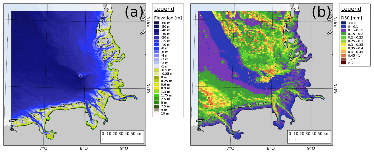
Figure 7Exemplary base products for 1996 for (a) bathymetry and (b) surface sedimentology painted as median grain diameter.

Figure 8Bathymetric gridded analysis products: (a) bed elevation range and (b) morphological drive.
2.4 Surface sediment porosity
As utilized in Eq. (3), the surface substrate porosity is an essential factor to consider in the development of the sedimentological surface composition of the ocean floor as generally a lower porosity leads to a denser material that has higher thresholds to erode and consequently leads to less change in elevation and thus, based on Eq. (3) sedimentological composition. As this is a model approach that is continuously developed and adjusted, we are aware that very well-sorted fine materials such as silt and clay actually increase their total porosity, yet as muds in our database of surface sediment samples tend to be moderately sorted or lower, we determined this effect to be negligible for the current application. Based on the parameters that can be extracted or extrapolated from the database, Eq. (6) is modified based on Wilson et al. (2018) to adjust porosity n for sorting coefficient σ in combination with the median grain size d50, where wc(d50) is the settling velocity based on Wu and Wang (2006).
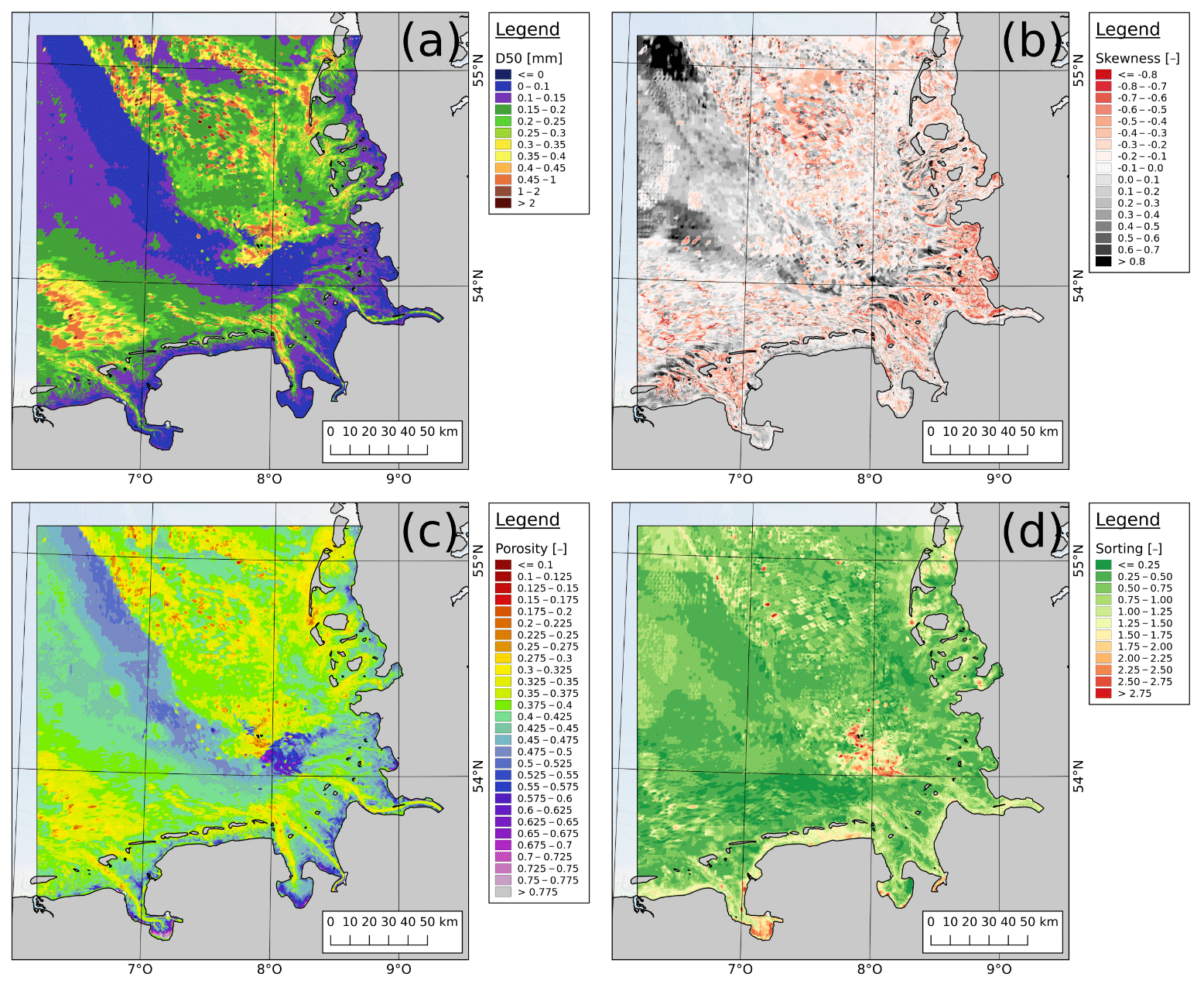
Figure 9Sedimentological analysis products for 1996: (a) median grain size d50, (b) skewness, (c) porosity, and (d) sorting coefficient.
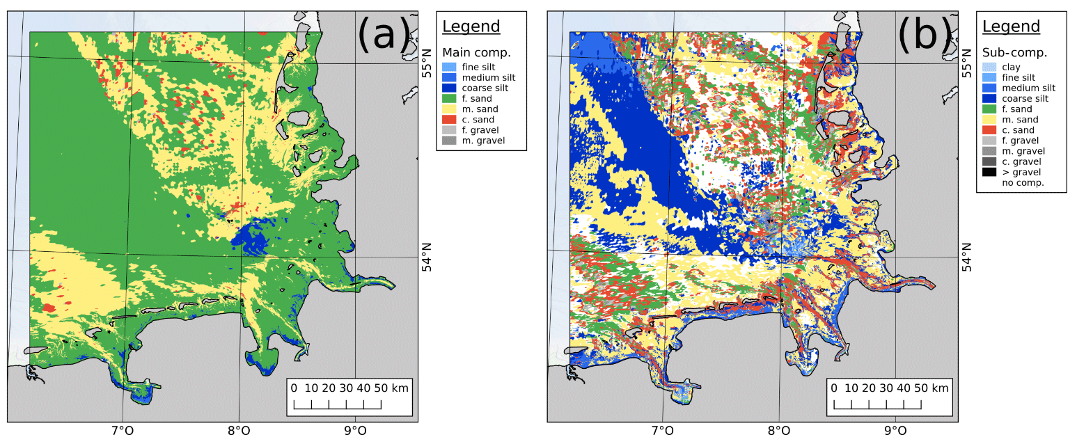
Figure 10Petrographical maps based on the abbreviated German SEP3 standard for 1996: (a) main components and (b) sub-component.
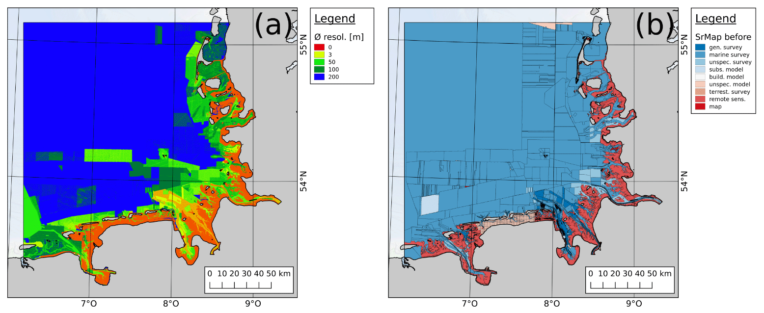
Figure 11Plausibility products for 2016: (a) data density map and (b) data source map (before) with the survey type as displayed attribute.
3.1 Gridded base products
By employing spatial and temporal interpolation as described in Sect. 2, the FSM was used to create 21 bathymetric digital terrain models (DTMs) for the German Bight ranging from 1996 to 2016 with validity dates on 1 July. Each DTM is provided as a structured grid with elevation data in a GeoTIFF format with a spatial grid resolution of 10 m (EPSG 25832). Furthermore, a 100 m structured grid of the EEZ is provided for 1 July 1996 (see Fig. 7a). As the DTMs have specific validity dates and not ranges, very short-term events like storm surges can only be accurately portrayed if their effects on bathymetric datasets is still noticeable at the model's validity date. Due to the FSM's ability to generate an elevation distribution for any given point in time, it would be possible to increase the temporal resolution of the DTMs to two, four, or even more models per year to potentially capture short-term catastrophic events. On the other hand, to capture long-term gradual events as best as possible, the 20 year time period (1996 to 2016) was specifically chosen to encompass the 18.6 year cycle of all constellations of Sun, Moon, and Earth that might influence tidal processes.
By employing spatial and temporal interpolation and extrapolation as described in Sect. 2, the FSM was used to generate three surface sedimentological models for the German Bight for 1996, 2006, and 2016, with validity dates on 1 July. Each surface sedimentological model is provided to users serving as a base dataset for individual analysis applications as a structured grid as a CSV file in EPSG 25832 with a spatial grid resolution of 100 m. Each file contains the model information in a 0.25 phi discretized cumulative GSD function, as well as coordinates and metadata such as date of validity. Furthermore, a 250 m structured grid of the EEZ is provided for 1 July 1996 (see Fig. 7b), represented by a further analysis of the cumulative function (see also later sections): the median grain size d50 is in millimeters.
3.2 Polygonal base products
Basic bathymetric and surface sedimentological information is in practice often utilized in the form of polygonal isolines. We thus generated isobaths for each bathymetric DTM in full spatial coverage in 0.5 m steps for high-resolution analyses and 10 m steps for general display purposes. Additionally, each median grain diameter (d50) gridded product is provided with polygonal representation as well. As the d50 is provided in metric scale, a logarithmic discretization for the isolines is required and utilized as defined by the German language version standard DIN EN ISO 14688 (Deutsches Institut für Normung, 2018), which defines grain size fractions on a logarithmic scale.
3.3 Gridded analysis products
Based on the DTM products, geomorphological analyses, i.e., the development of elevation, minimum and maximum elevation, and their range (termed the bed elevation range by Winter, 2011; Fig. 8a), are performed. The bed elevation range (BER), calculated as the range between the maximum and minimum elevation over the whole 20-year time period, gives an indication of high or low morphological activity. A high BER scalar value implies high morphological activity, which has to be taken into account when considering long-term stability for purposes of, for example, construction projects or planning of cable routes.
However, the BER cannot indicate rates of changes. The morphological drive (MD, Fig. 8b) instead analyzes not the absolute elevation range but the rates of change between sets of 2 consecutive years over the 20 year project period and portrays the range between the highest rate of change and the lowest rate of change. This helps assess whether an area was affected by gradual (e.g., tidal dynamics with low MD values) or sudden (e.g., storm surges with high MD values) influences. Especially when analyzed in conjunction with the BER, the MD can give valuable insight into the region's morphodynamical stability. A high BER with a low MD would indicate a large-scale but slow development, whereas the same high BER with a high MD would indicate a sudden change that took place within a short time span.
Further sedimentological analyses utilize the full cumulative GSD function from the base products. Based on grids with the same extent and resolution as the base products, the calculation of the median grain size d50 in millimeters, the sorting coefficient σ based on Folk (1980), the skewness coefficient Sk based on Folk (1980), and the porosity n (see Eq. (6)) were performed (Fig. 9).
3.4 Polygonal analytical products
For display purposes, sedimentological maps can be produced by a classification of grid points to their linguistic description of their respective cumulative GSD function. The concept of the generation of a (quasi-)bijective linguistic description from a function (Sievers and Milbradt, 2021) is based on a reversal of initial concepts from Voss (1982) and Naumann et al. (2014). It relies on the definition of grain size classes and respective percentages within the cumulative function relative to each other to determine a description that would adequately regenerate the original GSD function. With respect to mostly German stakeholders, the German description format “SEP3” based on grain size classification based on standards DIN 4022 and German language version DIN EN ISO 14688 (Deutsches Institut für Normung, 2011, 2018) is used as the target description structure.
While Voss (1982) and Naumann et al. (2014) solely focus on SEP3, the developed reversal of their process could be transferred to multiple other description formats as well. In a similar concept to the Figge grain size classification maps (Figge, 1981), the description is then split into main and sub-components to reduce the number of possible combinations to be displayed. The grid points of these datasets are then summarized into polygonal maps of main and sub-components.
A major advantage of these so called petrographical maps is that a cumulative GSD function can be reconstructed by recreating a full description from main and sub-component descriptions following Naumann et al. (2014) at every single point within the map without the need to store excessive spatial position data. For each base model, two sets of petrographical maps are created: one in the long, fully bijective form (i.e., a full description is stored) and a short form (i.e., only the first main and first sub-component is stored), which is displayed in Fig. 10.
Commonly, what datasets were used is not published with a DTM in its creation. A notable exception in this case is EMODnet Bathymetry (http://www.emodnet-bathymetry.eu, last access: 16 August 2021), for which the possibility to view certain metadata of datasets used for generating the DTM is provided. We aim to make the process of DTM generation fully transparent. As a consequence, each DTM itself generated by the FSM has specific metadata attached to it, which may give information about possibilities and limitations for certain users and their desired applications. They include common information such as
-
dataset title,
-
spatial extent and coordinate reference system, commonly in EPSG notation,
-
elevation range and height reference system, commonly in linguistic notation,
-
short description for potential additional information,
-
interpolation or approximation methods optimal for this dataset and possible parameters,
-
data provider and their contact information,
-
date or time span of validity.
Additionally, the FSM has the ability to further provide metadata that allow for an evaluation of validity and reliability of the DTM. We supply data density maps and a set of data source maps, which are provided with each single DTM as separate datasets.
4.1 Data density maps
Data density maps are gridded datasets in identical extent and resolution to their DTM and hold information about the spatial resolution of the underlying spatiotemporally interpolated bathymetric surveys (Fig. 11a). The definition of resolution of a field survey is based on their structure (see Fig. 3). For bilinear grids it is determined to be the grid cell length, for unstructured datasets with elements it is the mean edge length or elements connected to the point, and for unstructured datasets without elements it is the search radius as defined in the interpolation or approximation method (e.g., Shepard interpolation). A low value is thus equivalent to a high resolution and is usually correlated with a higher quality as they tend to be from newer datasets close to or on land and are generally measured with more precise technology with relatively low uncertainty or error, such as airborne laser scanning or multi-beam hydrographic surveys.
4.2 Data source maps
Data source maps are polygonal datasets which hold the metadata of the survey datasets used for spatiotemporal interpolation of each individual point inside a DTM. As previously explained, spatiotemporal interpolation in the FSM utilizes two datasets for each point before and after the interpolation date; thus two data source maps for datasets used before and after the interpolation date, respectively, are provided. To reliably trace the provenance of a single elevation value within the DTM, both maps are to be considered. In this context, the provided metadata for each dataset utilized in interpolation are as follows: (1) unique identifying IDs within the FSM, (2) the name of the dataset, (3) type and subtype of datasets (implicitly defining interpolation or approximation methods), (4) data source organizations, and (5) date or time span of validity (see Fig. 11b). Especially the date or time span of validity is of high interest as greater temporal distances to older and younger datasets employed in spatiotemporal interpolation may imply lower reliability for a specific area compared to other areas in the DTM with lesser distances. Data source maps are an especially valuable tool for general quality assurance of a DTM as potential implausible elevation values in the DTM can be traced back to the original survey datasets, in which a correction of potentially erroneous information may be performed.
The generation of the data source map as such takes place during the spatiotemporal interpolation of the DTM when each point of the model is individually handled. Attached to the calculation of the elevation itself, the metadata of the older and younger datasets used are stored in a grid of equal size and resolution as the DTM. After the DTM is successfully generated, an algorithm creates boundary polygons for each metadata group which adhere to common multi-polygon logic in that a polygon shell can have holes that contain another metadata polygon. The traceability of density, interpolation method, and source dataset for each individual elevation value of each DTM provides in our belief full transparency regarding potential user applications.
All datasets are open access and available for download as GeoTIFF/ESRI shape files (geomorphology and bathymetry: https://doi.org/10.48437/02.2020.K2.7000.0001, Sievers et al., 2020a; sedimentology: https://doi.org/10.48437/02.2020.K2.7000.0005, Sievers et al., 2020b) and additionally as web map (WMS), web feature (WFS), and web coverage services (WCSs) for direct integration into a GIS application:
-
Geomorphology and bathymetry WMS: https://mdi-dienste.baw.de/geoserver/EasyGSH_Bathymetrie/wms (last access: 16 August 2021)
-
Geomorphology and bathymetry WFS: https://mdi-dienste.baw.de/geoserver/EasyGSH_Bathymetrie/wfs (last access: 16 August 2021)
-
Geomorphology and bathymetry WCS: https://mdi-dienste.baw.de/geoserver/EasyGSH_Bathymetrie/wcs (last access: 16 August 2021)
-
Surface sedimentology WMS: https://mdi-dienste.baw.de/geoserver/EasyGSH_Sediment/wms (last access: 16 August 2021)
-
Surface sedimentology WFS: https://mdi-dienste.baw.de/geoserver/EasyGSH_Sediment/wfs (last access: 16 August 2021)
-
Surface sedimentology WCS: https://mdi-dienste.baw.de/geoserver/EasyGSH_Sediment/wcs (last access: 16 August 2021)
The project website (https://mdi-de.baw.de/easygsh/, last access: 12 March 2021) additionally provides a preview web application for the presented datasets.
The produced data are at the time of writing of this publication temporally and spatially the most consistent and continuous available with the highest temporal and spatial resolution and versatility for the German Bight as no fixed interpretation especially in surface sedimentological data is applied. Numerous new methodologies and validation approaches were developed and implemented, such as the morphological drive and petrographical surface sediment maps. The described Functional Seabed Model (FSM), as a data-based hindcast simulation model for the bathymetric development of the subaquatic surface and its sedimentological composition, was formed and expanded over a time span of over a decade. As it was designed to be highly modular, it can therefore be expanded with new components very easily. Currently, the integration of the subsurface sediment composition of the morphologically active or activatable space is under development (see methodology excerpt in the conference presentation of Sievers et al., 2020) in the publicly funded KFKI project “Stratigraphic Model Components for the Improvement of High-Resolution and Regionalized Morphodynamic Simulation Models” (SMMS) in cooperation with the German Federal Waterways Engineering and Research Institute and the Federal Maritime and Hydrographic Agency of Germany. SMMS aims to provide consistent and continuous stratigraphical data of the sub-seafloor and adjacent estuaries to further improve the ability of hydrodynamic numerical model systems to assess erosional processes. Additionally, ecological model components (see methodology excerpt in the conference presentation of Rubel et al., 2021) are developed in connection with the publicly funded KFKI project “Roughness effects of oyster reefs and blue mussel beds in the German Wadden Sea” (BIVA-WATT). With this, we aim to be able to provide the most comprehensive synoptic base and validation data for numerous morphodynamic model systems and other general applications.
JS contributed to article composition, article figures, article concept, conceptual product design, implementation, and product generation. PM contributed to project initiation, supervision, proofreading, article concept, conceptual product design, and implementation. RI contributed to metadata and repository management and digital object identifier registration. JV contributed to project initiation, proofreading, and base data provision. RH contributed to the coordination of Part 1 and Part 2, applicability analyses of products, proofreading, and article concept. AP contributed to project initiation, supervision, and applicability analyses of products.
The authors declare that they have no conflict of interest.
Publisher's note: Copernicus Publications remains neutral with regard to jurisdictional claims in published maps and institutional affiliations.
We thank the German Federal Ministry of Transport (BMVI) for funding the mFUND project EasyGSH-DB, which has made this report and every data product presented herein possible. We would like to express our gratitude to all EasyGSH-DB collaborators which are the Federal Waterways Engineering and Research Institute, Germany (BAW), Küste und Raum, and the Federal Maritime and Hydrographic Agency, Germany (BSH), for their valuable input and enjoyable corroboration. We would also like to acknowledge the many stakeholders which have provided constant feedback to us and contributed their time to improve our data products presented herein. The bathymetric DTM in the form of a Web Map Service used as background maps in map overview figures has been derived from the EMODnet Bathymetry portal – http://www.emodnet-bathymetry.eu (last access: 16 August 2021). Julian Sievers and Peter Milbradt also thank Malte Rubel for discussions regarding sedimentological products and Diego Felipe Pineda Leiva for further proofreading.
This research has been supported by the Bundesministerium für Verkehr und Digitale Infrastruktur (grant no. 19F2004A-D).
This paper was edited by Giuseppe M. R. Manzella and reviewed by two anonymous referees.
Arns, A., Wahl, T., Dangendorf, S., and Jensen, J.: The impact of sea level rise on storm surge water levels in the northern part of the German Bight, Coast. Eng., 96, 118–131, https://doi.org/10.1016/j.coastaleng.2014.12.002, 2015.
Benninghoff, M. and Winter, C.: Recent morphologic evolution of the German Wadden Sea, Sci. Rep.-UK, 9, 1–9, https://doi.org/10.1038/s41598-019-45683-1, 2019.
DIN 18123-1:2011-04, Baugrund, Untersuchung von Bodenproben – Bestimmung der Korngrößenverteilung, Deutsches Institut für Normung, 2011.
DIN EN ISO 14688-1:2018-05, Geotechnische Erkundung und Untersuchung – Benennung, Beschreibung und Klassifizierung von Boden – Teil 1: Benennung und Beschreibung, Deutsches Institut für Normung, 2018.
Elias, E. P., Van der Spek, A. J., Wang, Z. B., and De Ronde, J.: Morphodynamic development and sediment budget of the Dutch Wadden Sea over the last century, Neth. J. Geosci., 91, 293–310, https://doi.org/10.1017/S0016774600000457, 2012.
Figge, K.: Sedimentverteilung in der Deutschen Bucht, Karte Nr. 2900 (mit Begleitheft), Deutsches Hydrographisches Institut, 1981.
Folk, R. L.: Petrology of sedimentary rocks, Hemphill Publishing Company, Austin, USA, 1980.
Gallagher, E. L., Elgar, S., and Guza, R. T.: Observations of sand bar evolution on a natural beach, J. Geophys. Res.-Oceans, 103, 3203–3215, https://doi.org/10.1029/97JC02765, 1998.
Genchi, S. A., Vitale, A. J., Perillo, G. M., Seitz, C., and Delrieux, C. A.: Mapping topobathymetry in a shallow tidal environment using low-cost technology, Remote Sens.-Basel, 12, 1394, https://doi.org/10.3390/rs12091394, 2020.
Hagen, R., Freund, J., Plüß, A., and Ihde, R.: Validierungsdokument EasyGSH-DB Nordseemodell. Teil UnTRIM2 – SediMorph – UnK, BAW Technischer Bericht B3955.02.04.70229.1, Bundesanstalt für Wasserbau, https://doi.org/10.18451/k2_easygsh_1, 2020.
Hagen, R., Plüß, A., Ihde, R., Freund, J., Dreier, N., Nehlsen, E., Schrage, N., Fröhle, P., and Kösters, F.: An integrated marine data collection for the German Bight – Part 2: Tides, salinity, and waves (1996–2015), Earth Syst. Sci. Data, 13, 2573–2594, https://doi.org/10.5194/essd-13-2573-2021, 2021.
Heyer, H. and Schrottke, K.: Einführung, Aufgabenstellung und Bearbeitungsstruktur im KFKI-Projekt, Die Küste, 83 AufMod, 1–18, https://doi.org/10.18171/1.083000, 2015.
Kabat, P., Bazelmans, J., van Dijk, J., Herman, P. M., van Oijen, T., Pejrup, M., Reise, K., and Speelman, H. W.: The Wadden Sea Region: Towards a science for sustainable development, Ocean Coast. Manage., 68, 4–17, https://doi.org/10.1016/j.ocecoaman.2012.05.022, 2012.
Kirichek, A., Chassagne, C., Winterwerp, H., and Vellinga, T.: How navigable are fluid mud layers?, Terra et Aqua: International Journal on Public Works, Ports and Waterways Developments, 20, 2546–2552, 2018.
Kirichek, A., Shakeel, A., and Chassagne, C.: Using in situ density and strength measurements for sediment maintenance in ports and waterways, J. Soil. Sediment., 20, 2546–2552, https://doi.org/10.1007/s11368-020-02581-8, 2020.
Kösters, F. and Winter, C.: Exploring German Bight coastal morphodynamics based on modelled bed shear stress, Geo-Mar. Lett., 34, 21–36, https://doi.org/10.1007/s00367-013-0346-y, 2014.
Kuusela, M. and Stein, M. L.: Locally stationary spatio-temporal interpolation of Argo profiling float data, P. Roy. Soc. A-Math. Phy., 474, 20180400, https://doi.org/10.1098/rspa.2018.0400, 2018.
Milbradt, P., Valerius, J., and Zeiler, M.: Das funktionale Bodenmodell: Aufbereitung einer konsistenten Datenbasis für die Morphologie und Sedimentologie, Die Küste, 83 AufMod, 19–38, https://doi.org/20.500.11970/101736, 2015.
Moulton, M., Elgar, S., and Raubenheimer, B.: Improving the time resolution of surfzone bathymetry using in situ altimeters, Ocean Dynam., 64, 755–770, https://doi.org/10.1007/s10236-014-0715-8, 2014.
Naumann, M., Waldeck, A., Poßin, W., and Schwarz, C. F.: Ableitung von Korngrößenverteilungen aus textbasierten petrografischen Bohrgutbeschreibungen, Z. Dtsch. Ges. Geowiss., 165, 275–286, https://doi.org/10.1127/1860-1804/2014/0056, 2014.
Rasquin, C., Seiffert, R., Wachler, B., and Winkel, N.: The significance of coastal bathymetry representation for modelling the tidal response to mean sea level rise in the German Bight, Ocean Sci., 16, 31–44, https://doi.org/10.5194/os-16-31-2020, 2020.
Roeland, H. and Piet, R.: Dynamic preservation of the coastline in the Netherlands, J. Coast. Conserv., 1, 17–28, https://doi.org/10.1007/BF02835558, 1995.
Rubel, M., Ricklefs, K., Milbradt, P., and Sievers, J.: A model approach to estimate the potential for mussel beds in a Wadden Sea area of the German North Sea coast, EGU General Assembly 2020, Online, 4–8 May 2020, EGU2020-3574, https://doi.org/10.5194/egusphere-egu2020-3574, 2020.
Sievers, J. and Milbradt, P.: Quasi-bijective mapping of linguistic sediment description and cumulative grain size distribution functions, in preperation, 2021.
Sievers, J., Milbradt, P., and Rubel, M.: Databased simulation and reconstruction of the near shore geomorphological structure and sediment composition of the German tidal flats, EGU General Assembly 2020, Online, 4–8 May 2020, EGU2020-2566, https://doi.org/10.5194/egusphere-egu2020-2566, 2020.
Sievers, J., Rubel, M., and Milbradt, P.: EasyGSH-DB: Themengebiet – Geomorphologie, Bundesanstalt für Wasserbau [data set], https://doi.org/10.48437/02.2020.K2.7000.0001, 2020a.
Sievers, J., Rubel, M., and Milbradt, P.: EasyGSH-DB: Themengebiet – Sedimentologie, Bundesanstalt für Wasserbau [data set], https://doi.org/10.48437/02.2020.K2.7000.0005, 2020b.
Tauber, F.: Treating grain-size data as continuous functions, Proceedings of IAMG 97, 169–174, 1997.
Voss, H.-H.: Unterlagen über Material und Methoden zur Vereinheitlichung der Korngrößenansprache bei der geologischen und bodenkundlichen Landesaufnahme, Archivber. Nr. 010930, Niedersächsisches Landesamt für Bodenforschung, 1982.
Wang, S., Dieterich, C., Döscher, R., Höglund, A., Hordoir, R., Meier, H. M., and Samuelsson, P. S.: Development and evaluation of a new regional coupled atmosphere–ocean model in the North Sea and Baltic Sea, Tellus A, 67, 24284, https://doi.org/10.3402/tellusa.v67.24284, 2015.
Wang, Z. B., Elias, E. P., van der Spek, A. J., and Lodder, Q. J.: Sediment budget and morphological development of the Dutch Wadden Sea: impact of accelerated sea-level rise and subsidence until 2100, Neth. J. Geosci., 97, 183–214, https://doi.org/10.1017/njg.2018.8, 2018.
Wilson, R. J., Speirs, D. C., Sabatino, A., and Heath, M. R.: A synthetic map of the north-west European Shelf sedimentary environment for applications in marine science, Earth Syst. Sci. Data, 10, 109–130, https://doi.org/10.5194/essd-10-109-2018, 2018.
Winter, C.: Macro scale morphodynamics of the German North Sea coast, J. Coast. Res., 57, 706–710, 2011.
Wölfl, A.-C., Snaith H., Amirebrahimi S., Devey C. W., Dorschel B., Ferrini V., Huvenne V. A. I., Jakobsson M., Jencks J., Johnston G., Lamarche G., Mayer L., Millar D., Pedersen T. H., Picard K., Reitz A., Schmitt T., Visbeck M., Weatherall P., and Wigley R.: Seafloor Mapping – The Challenge of a Truly Global Ocean Bathymetry, Front. Mar. Sci., 6:283, https://doi.org/10.3389/fmars.2019.00283, 2019.
Wu, W. and Wang, S. S.: Formulas for sediment porosity and settling velocity, J. Hydraul. Eng., 858–862, https://doi.org/10.1061/(ASCE)0733-9429(2006)132:8(858), 2006.
Zijl, F., Verlaan, M., and Gerritsen, H.: Improved water-level forecasting for the Northwest European Shelf and North Sea through direct modelling of tide, surge and non-linear interaction, Ocean Dynam., 63, 823–847, https://doi.org/10.1007/s10236-013-0624-2, 2013.
- Abstract
- Introduction
- The methodological framework of the Functional Seabed Model (FSM)
- Products
- Plausibility evaluation products for gridded bathymetric base products
- Data availability
- Conclusions and outlook
- Author contributions
- Competing interests
- Disclaimer
- Acknowledgements
- Financial support
- Review statement
- References