Long time series of daily evapotranspiration in China based on the SEBAL model and multisource images and validation

Satellite observations of evapotranspiration (ET) have been widely used for water resources management in China. An accurate ET product with a high spatiotemporal resolution is required for research on drought stress and water resources management. However, such a product is currently lacking. Moreover, the performances of different ET estimation algorithms for China have not been clearly studied, especially under different environmental conditions. Therefore, the aims of this study were as follows: (1) to use multisource images to generate a long-time-series (2001–2018) daily ET product with a spatial resolution of 1 km × 1 km based on the Surface Energy Balance Algorithm for Land (SEBAL); (2) to comprehensively evaluate the performance of the SEBAL ET in China using flux observational data and hydrological observational data; and (3) to compare the performance of the SEBAL ET with the MOD16 ET product at the point scale and basin scale under different environmental conditions in China. At the point scale, both the models performed best in the conditions of forest cover, subtropical zones, hilly terrain, or summer, respectively, and SEBAL performed better in most conditions. In general, the accuracy of the SEBAL ET (rRMSE = 44.91 %) was slightly higher than that of the MOD16 ET (rRMSE = 48.72 %). In the basin-scale validation, both the models performed better than in the point-scale validation, with SEBAL obtaining results superior (rRMSE = 13.57 %) to MOD16 (rRMSE = 32.84 %). Additionally, both the models showed a negative bias, with the bias of the MOD16 ET being higher than that of the SEBAL ET. In the daily-scale validation, the SEBAL ET product showed a root mean square error (RMSE) of 0.92 mm d⁻¹ and an r value of 0.79. In general, the SEBAL ET product can be used for the qualitative analysis and most quantitative analyses of regional ET. The SEBAL ET product is freely available at https://doi.org/10.5281/zenodo.4243988 and https://doi.org/10.5281/zenodo.4896147 (Cheng, 2020a, b). The results of this study can provide a reference for the application of remotely sensed ET products and the improvement of satellite ET observation algorithms.

1 Introduction

Evapotranspiration (ET) is the process of transferring surface water to the atmosphere, including soil evaporation and vegetation transpiration (Wang and Dickinson, 2012). This process is a key node linking surface water and energy balance. In the process of water balance, ET represents the consumption of surface water resources, and in the process of energy balance, the energy consumed by ET is called the latent heat flux (λET, W m⁻², where λ is the latent heat vaporization), which is an important energy component (Helbig et al., 2020; Zhao et al., 2019). Approximately 60 % of global precipitation ultimately returns to the atmosphere through evapotranspiration (Wang and Dickinson, 2012). Therefore, accurately quantifying the ET of different land cover types is necessary to better understand changes in regional water resources. However, the methods for the estimation of ET based on point-scale or small-area-scale analysis, such as lysimeters and eddy covariance, cannot meet the requirement of global climate change research and regional water resource management (Li et al., 2018). Since the United States successfully launched the first meteorological satellite in the 1960s, hydrological remote sensing (RS) applications have developed rapidly and have led to huge breakthroughs (Karimi and Bastiaanssen, 2015). Remote sensing technology with a high spatiotemporal continuity provides an effective means for regional ET estimation.

Satellite remote sensing provides a reliable direct estimation of ground parameters; however, it cannot measure ET directly (Wang and Dickinson, 2012). Therefore, several RS-based algorithms for the estimation of ET have been proposed and reviewed (Pôças et al., 2020; Senay et al., 2020; Wang and Dickinson, 2012). These models can be divided into three types according to their mechanism: those based on surface energy balance residual (SEBR), those based on semi-empirical formulas (SEFs), and statistic methods. SEBR-based models can be further divided into one-source models and two-source models (Wang and Dickinson, 2012). One-source models do not distinguish vegetation from bare soil and regard the land surface as a system that exchanges energy and water with the atmosphere. Examples of one-source models include the Surface Energy Balance Index (S-SEBI) (Roerink et al., 2000), the Surface Energy Balance System (SEBS) (Su, 1999), and the Surface Energy Balance Algorithm for Land (SEBAL) (Bastiaanssen et al., 1998a, b). These models have a theoretical basis, a simple principle, and strong portability, and they have been widely used (Bastiaanssen and Steduto, 2017; Elnmer et al., 2019; Huang et al., 2015; Wagle et al., 2019). Two-source models distinguish the surface water and energy exchange between vegetation and bare soil and calculate fractional canopy coverage (F_c) using an empirical formula and a vegetation index obtained from remote sensing data to divide the land surface into vegetation and bare soil in each single pixel. Examples of two-source models include the the Two-Source Energy Balance (TSEB) model (Kustas et al., 2003), the Two-source Trapezoid Model for Evapotranspiration (TTME) (Long and Singh, 2012), and the Hybrid Dual-source Scheme and Trapezoid Framework-based Evapotranspiration Model (HTEM) (Yang and Shang, 2013). Compared to one-source models, two-source models have a superior theoretical mechanism. SEF-based models using traditional semi-empirical formulas calculate λET and are simpler than SEBR-based models. Examples of SEF-based models include the Surface Temperature and Vegetation Index (T_s–VI) space model (Carlson, 2007) and the Global Land Evaporation Amsterdam Model (GLEAM) based on the Priestley–Taylor (P–T) equation (Miralles et al., 2011). Another well-known SEF-based model is based on the Penman–Monteith (P–M) equation, which has been improved and applied to remote sensing data to estimate regional ET (Mu et al., 2007, 2011). Moreover, statistic methods for ET estimation by using statistical regression or machine learning to fit multiple indicators (e.g., meteorological data or remote sensing data) and in situ ET are also being widely used (Mosre and Suárez, 2021; Yamaç and Todorovic, 2020).

Since ET plays a critical role in the study of hydrology and ecology, ET products with a high spatiotemporal resolution are required. Therefore, a growing number of ET products have been generated to meet research needs. These include MOD16, which is generated by NASA based on the Penman–Monteith algorithm and has a spatial resolution of 500 m × 500 m and a temporal resolution of 8 d (Mu et al., 2007, 2011). The GLEAM daily ET product with a spatial resolution of 0.25^∘ × 0.25^∘ has been generated by the University of Bristol, UK, based on the Priestley–Taylor method (Miralles et al., 2010). Additionally, Chen generated long-time-series daily ET datasets with a spatial resolution of 0.1^∘ × 0.1^∘ based on the SEBS algorithm (X. Chen et al., 2014; Chen, 2019). However, there are few ET products that simultaneously meet the current research needs in terms of temporal and spatial resolution. Therefore, generating a kilometer-level daily ET product that can minimize the influence of mixed pixels is critical.

Water resources management is essential for China as it has an unbalanced spatial and temporal distribution of water resources. ET, as a crucial component of the terrestrial water cycle, is critical for understanding the water resources budget in China. Therefore, spatiotemporally continuous ET data are needed. Several studies evaluated the performance of various remote-sensing-based algorithms in China. For example, Y. Chen et al. (2014) used 23 eddy covariance (EC) sites to evaluate the performance of the Penman–Monteith method (used for generating the MOD16 product) and the Priestley–Taylor method (used for generating the GLEAM product) in China; however, these models can only explain approximately 61 %–80 % of the variability in ET. Li et al. (2017) used an SEBR-based model – SEBS – to map the ET in Heihe River Basin, northwestern China, and evaluated its performance in different land cover types. In general, SEBS outperformed the Priestley–Taylor method, but SEBS showed significant bias in several land cover types, e.g., village (mainly croplands). Sun et al. (2020) evaluated the performance of Shuttleworth–Wallace–Hu (SWH) and SEBAL in northwestern China and showed better accuracy than the MOD16 product. In general, the accuracy of ET derived from satellite imagery is affected by spatiotemporal conditions (Wagle et al., 2017). Several studies have indicated that RS-based methods for modeling ET have errors of 15 %–50 % (Velpuri et al., 2013; Xue et al., 2020). RS-based models have different applicable conditions, and understanding the variation in accuracy between such models is important for their reasonable application. However, few studies have validated the robustness of different models using long time series and at a large spatial scale. For China with a large area and complex terrain, few studies have clearly discussed the performance of RS-based models under different environmental conditions, and most studies only aimed at a certain area. Moreover, there is no ET product for China with a high spatiotemporal resolution, and the applicability of different RS-based models for the estimation of ET in China is not clear, which hampers the management of ET.

In order to improve ET products in China and better understand the performance of RS-based ET estimation models in China, in this paper, we aim to (1) generate a long-time-series daily ET product with a spatial resolution of 1 km × 1 km based on the SEBAL model and multisource remote sensing images, (2) validate the accuracy of the generated ET product in China based on flux tower observational data and hydrological data, and (3) compare the performance of the generated ET product with MOD16 datasets in China under different environmental conditions.

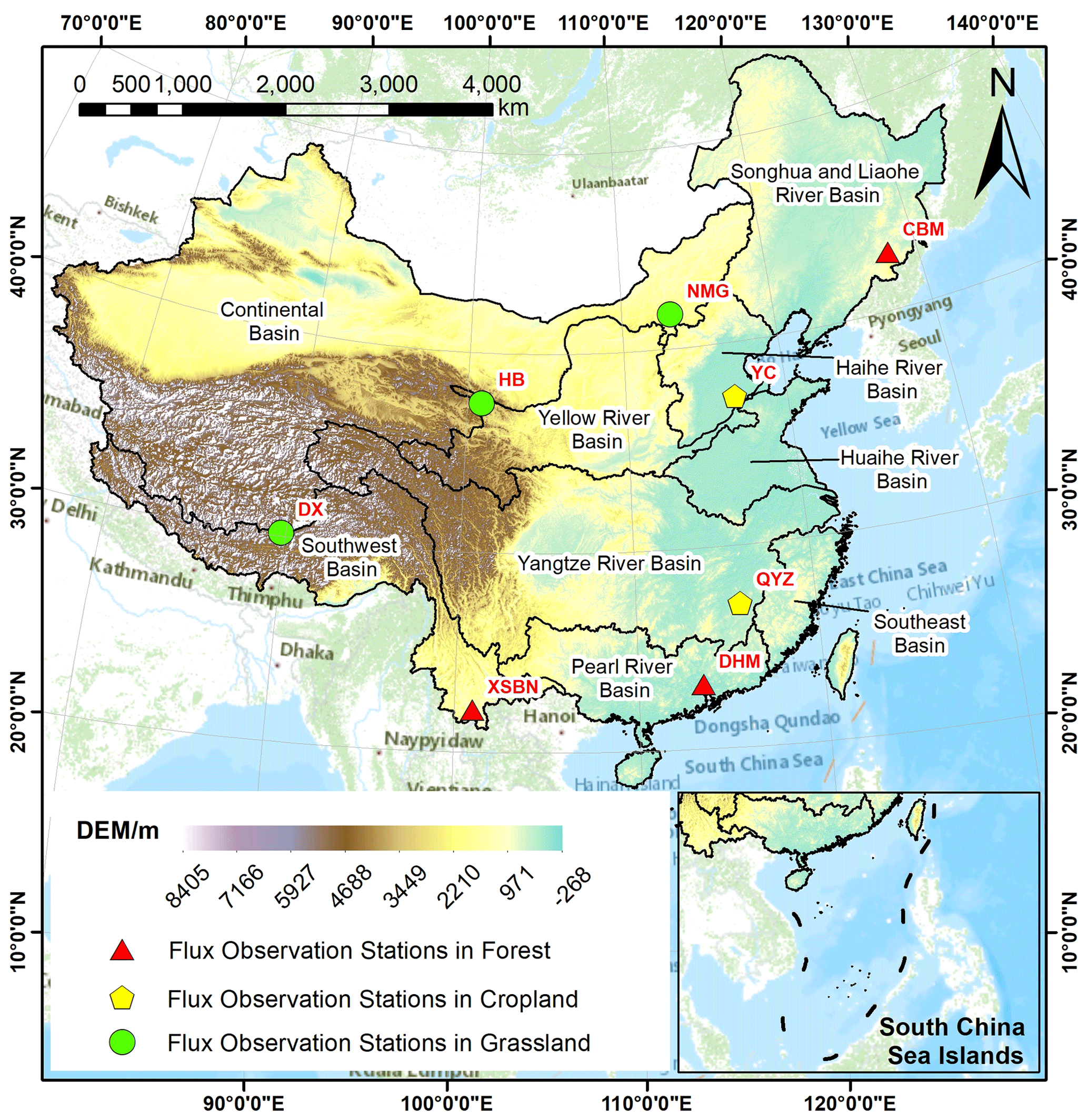
Figure 1 The location of the study area. CBM: Changbai mountain; DHM: Dinghu mountain; DX: Dangxiong; HB: Haibei; NMG: Neimenggu; QYZ: Qianyanzhou; XSBN: Xishuangbanna; YC: Yucheng. Please note that the above figure contains disputed territories. Note: Chinese boundaries were obtained from the Institute of Geographic Science and Natural Resources Research, Chinese Academy of Sciences: http://www.resdc.cn/ (last access: July 2021).

2 Materials and methods

2.1 Study area

China (3^∘31^′00^′′–53^∘33^′47^′′ N, 73^∘29^′59.79^′′–135^∘2^′30^′′ E) covers a land area of approximately 9 600 000 km², mainly including temperate zones, warm–temperate zones, subtropical zones, tropical zones, and plateau climate zones. China can be divided into nine basin regions based on the distribution of water resources (Zhang et al., 2011): the Southwest Basin (SwB), Continental Basin (CB), Pearl River Basin (PRB), Yangtze River Basin (YRB), Southeast Basin (SeB), Haihe River Basin (HRB), Yellow River Basin (YeRB), Huaihe River Basin (HuRB), and Songhua and Liaohe River Basin (SLRB) (Fig. 1).

Figure 2 A flowchart of the Surface Energy Balance Algorithm for Land (SEBAL), which was used to convert multisource images to daily evapotranspiration.

2.2 Generation of a long-time-series daily ET product

In this study, a long-time-series daily ET product was generated based on SEBAL, which is a widely used one-source model (Gobbo et al., 2019; Jaafar and Ahmad, 2020; Mhawej et al., 2020; Rahimzadegan and Janani, 2019). SEBAL has been shown to have a good performance for ET estimation and can be regarded as typical of SEBR-based models (Bastiaanssen et al., 1998b; Timmermans et al., 2006; Wagle et al., 2017). The workflow for the calculation of the daily ET using the SEBAL model and multisource satellite images is shown in Fig. 2. The SEBAL model calculates the instantaneous λET of the satellite transit time as a residual based on the surface energy balance equation (Eq. 1) as follows:

$$\begin{array}{}\text{(1)}& \mathit{\lambda }\text{ET}=R_{\mathrm{n}}-G-H,\end{array}$$

where R_n is the net radiation flux, H is the sensible heat flux, and G is the soil heat flux (the unit of all three parameters is W m⁻²). In this paper, MODIS data (MCD43 surface albedo, MOD11 surface temperature – daytime, MOD13 NDVI) and meteorological data (air temperature) from the Global Modeling and Assimilation Office (GMAO) were used as input for surface parameterization (R_n, G, and H). The details of generating SEBAL ET can be found in Appendix A.

The spatial and temporal resolutions of the MCD43 surface albedo and the MOD11 daytime surface temperature are 1 d and 1 km × 1 km, while those of MOD13 NDVI are 16 d and 500 m × 500 m. In this study, MOD13 was resampled to 1 km × 1 km and processed by smoothing and gap filling from time series to daily data (Vuolo et al., 2017). It should be noted that there are several missing or unreliable pixels in MODIS images, which may be caused by clouds or other reasons; these pixels were marked in quality control (QC) files. In this study, these anomalous pixels of the MODIS dataset (MOD11, MOD13, and MCD43) were filled by referring to previous studies, with the rules as follows: (1) the value of an anomalous pixel will be computed by liner interpolation of the nearest reliable value after it or prior to it; (2) if the anomalous pixel was found in the first or last day, it will be replaced by the closest reliable date value. More details can be found in the studies of Mu et al. (2011) and Zhao et al. (2005). Land surface temperature is the crucial parameter for SEBAL ET generation, and Appendix B shows the ratio of interpolated pixels of land surface temperature (MOD11) data (31 % ± 11 %). The spatial and temporal resolutions of GMAO air temperature are 1 d and 0.25^∘ × 0.25^∘, respectively. The coarse-resolution GMAO data were nonlinearly interpolated to a spatial resolution of 1 km × 1 km based on the four GMAO pixels surrounding a given pixel (Zhao et al., 2005). The spatial and temporal resolutions of wind speed are 1 d and 1 km × 1 km (China Meteorological Data Network, http://data.cma.cn, last access: July 2021). The final generated daily ET product has a spatial resolution of 1 km × 1 km and covers the period 2001 to 2018.

Table 1 Details of the eight flux observation stations.

2.3 Validation methods

2.3.1 Point-scale validation

The eddy covariance method measures λET from the covariance between moisture fluxes and vertical wind velocity using rapid response sensors at frequencies typically equal to or greater than 10 Hz (Wang and Dickinson, 2012); it is regarded as the most effective method for the estimation of ET and has been widely used (Wang and Dickinson, 2012). In this study, eddy covariance tower-measured daily flux data from eight stations in China (Table 1) obtained in 2003–2010 were used to validate the modeled ET (ET_SEBAL, ET_MOD). The latent heat flux (λET) observed at the flux towers was converted into the observed ET (ET_flux). It should be noted that the energy balance closure issue, which indicates that the sum of sensible heat (H), latent heat (λET), and soil heat flux (G) is not equal to net radiation (R_n), was often found in the eddy covariance system. Therefore, the eddy covariance system measured value should be filtered and corrected. First, the data with an energy balance closure ratio (ECR, Eq. 2) less than 80 % were not selected for validation (Wang et al., 2019), and then the remaining data with an ECR more than 80 % were corrected by using the Bowen ratio energy balance correction (Eq. 3) (Y. Chen et al., 2014).

$$\begin{array}{}\text{(2)}& {\displaystyle }\text{ECR}={\displaystyle \frac{H+\mathit{\lambda }\text{ET}}{R_{\mathrm{n}}-G}}\text{(3)}& {\displaystyle }\mathit{\lambda }{\text{ET}}_{\text{cor}}={\displaystyle \frac{R_{\mathrm{n}}-G}{H+\mathit{\lambda }\text{ET}}}\cdot \mathit{\lambda }\text{ET}\end{array}$$

Here, R_n, G, H, and λET are all eddy covariance system measured values, and λET_cor is the corrected value. To ensure a reliable evaluation, the pixel value where the flux tower is located (area of 1 km × 1 km) was extracted for comparison with the measured value (Velpuri et al., 2013). The water demand is different under different environmental conditions. Therefore, it is necessary to understand the accuracy performance of ET products for different vegetation types when a single ET product is not comprehensive (Velpuri et al., 2013). In order to better understand the influence of different environmental conditions on the accuracy of the model, the modeled ETs were validated for different terrain, climate zones, land cover types, and seasons. Additionally, MOD16 data were resampled to a spatial resolution of 1 km × 1 km, and daily ET_SEBAL and daily ET_flux data were accumulated to 8 d to match the MOD16 data. ET_SEBAL was validated at the daily scale and 8 d scale.

2.3.2 Regional-scale validation

Furthermore, the regional (basin-scale) ET was calculated using the water balance method (Eq. 4) to validate the modeled ET at the regional scale.

$$\begin{array}{}\text{(4)}& \text{ET}=P-Q-\mathrm{\Delta }S\end{array}$$

Here, P (unit: mm) is the annual precipitation in the basin, Q (unit: mm) is the annual runoff in the basin, which includes surface runoff and groundwater runoff, and ΔS is the change in the groundwater and surface water storage in a year; the change in ΔS over multiple years can be ignored (Liu et al., 2016; Senay et al., 2011). The average ET over multiple years was calculated in each primary water resources division in China (the nine basins shown in Fig. 1) from 2001 to 2018; these values of ET are referred to as ET_WB.

2.3.3 Accuracy estimation

The modeled ET values were compared with the observed ET (ET_flux, ET_WB) to evaluate the performance of ET_SEBAL and ET_MOD, respectively. The correlation coefficient (r), root mean square error (RMSE), relative root mean square error (rRMSE), and mean bias error (MBE) were selected to quantify the accuracy of the modeled ET. The equations for these parameters are shown below.

$$\begin{array}{}\text{(5)}& {\displaystyle }r={\displaystyle \frac{{\sum }_{i=\mathrm{1}}^n\left({\mathrm{ET}}_{\mathrm{M}\mathit{\text{i}}}-\stackrel{\mathrm{‾}}{{\mathrm{ET}}_{\mathrm{M}}}\right)\left({\mathrm{ET}}_{\mathrm{Ob}\mathit{\text{i}}}-\stackrel{\mathrm{‾}}{{\mathrm{ET}}_{\mathrm{Ob}}}\right)}{\sqrt{{\sum }_{i=\mathrm{1}}^n{\left({\mathrm{ET}}_{\mathrm{M}\mathit{\text{i}}}-\stackrel{\mathrm{‾}}{{\mathrm{ET}}_{\mathrm{M}}}\right)}^{\mathrm{2}}{\sum }_{i=\mathrm{1}}^n{\left({\mathrm{ET}}_{\mathrm{Ob}\mathit{\text{i}}}-\stackrel{\mathrm{‾}}{{\mathrm{ET}}_{\mathrm{Ob}}}\right)}^{\mathrm{2}}}}}\text{(6)}& {\displaystyle }\text{RMSE}=\sqrt{{\displaystyle \frac{\mathrm{1}}{n}}{\sum }_{i=\mathrm{1}}^n({\mathrm{ET}}_{\mathrm{M}\mathit{\text{i}}}-{\mathrm{ET}}_{\mathrm{Ob}\mathit{\text{i}}}{)}^{\mathrm{2}}}\text{(7)}& {\displaystyle }\text{rRMSE}={\displaystyle \frac{\text{RMSE}}{\stackrel{\mathrm{‾}}{{\mathrm{ET}}_{\mathrm{Ob}}}}}\cdot \mathrm{100}\mathit{\%}\text{(8)}& {\displaystyle }\text{MBE}={\displaystyle \frac{\mathrm{1}}{n}}{\sum }_{i=\mathrm{1}}^n({\mathrm{ET}}_{\mathrm{M}\mathit{\text{i}}}-{\mathrm{ET}}_{\mathrm{Ob}\mathit{\text{i}}})\end{array}$$

Here, ET_M is the modeled ET (ET_SEBAL and ET_MOD), ET_Ob is the observed ET (ET_flux and ET_WB), and n is the number of samples. r was calculated to evaluate the linear relationship between the modeled and observed ET; higher r values mean a higher correlation. RMSE and rRMSE were used to evaluate the performance of the model: smaller RMSE and rRMSE mean higher accuracy. The rRMSE is a critical indicator to evaluate the accuracy of a model (Jin et al., 2020). The MBE was used to measure whether the result was overestimated (positive values of MBE) or underestimated (negative values of MBE).

2.4 Data sources and tools used

2.4.1 MOD16 data

The MOD16 ET product is a widely used evapotranspiration dataset for water resources management and global change study, which also performs accurately to some extent (He et al., 2019; Mu et al., 2011). In this study, the comparison of SEBAL ET and MOD16 ET was conducted to judge if further improvement was found in SEBAL ET. The MOD16 ET data (ET_MOD) were produced using an ET algorithm based on the P–M equation (Eq. 9) (Monteith, 1965) that has been improved (Mu et al., 2007, 2011).

$$\begin{array}{}\text{(9)}& \mathit{\lambda }\text{ET}={\displaystyle \frac{sA+\mathit{\rho }{C}_{\mathrm{p}}\text{VPD}/r_{\mathrm{a}}}{s+\mathit{\gamma }(\mathrm{1}+r_{\mathrm{s}}/r_{\mathrm{a}})}}\end{array}$$

Here, s (unit: Pa K⁻¹) is the slope of the temperature-saturated water pressure curve at the current temperature, A (unit: W m⁻²) is the available energy, ρ (unit: kg m⁻³) is the air density, C_p (unit: $\mathrm{J}(\mathrm{kg}\cdot \mathrm{K}{)}^{-\mathrm{1}}$) is the specific heat of air at constant pressure, VPD (unit: Pa) is the difference in water vapor pressure, γ (unit: Pa K⁻¹) is the psychrometric constant, and r_a and r_s (unit: s m⁻¹) are the aerodynamic resistance and surface resistance, respectively. The MOD16 ET data are available for regular 500 m grid cells for the entire global vegetated land surface at 8 d composite, and the data do not cover regions corresponding to water, barren land, and buildings (He et al., 2019). In this study, MOD16 data were obtained from the NASA Atmosphere Archive and Distribution System Distributed Active Archive Center (LAADS DAAC, https://ladsweb.modaps.eosdis.nasa.gov, last access: July 2021).

2.4.2 Auxiliary data

In order to ensure the objectivity of the comparison between the SEBAL and P–M models, MODIS satellite data were selected as the input for SEBAL, including the surface albedo (MCD43), surface temperature (MOD11), and NDVI (MOD13) obtained from LAADS DAAC. Additionally, gridded air temperature data were obtained from the GMAO (https://gmao.gsfc.nasa.gov, last access: July 2021). Flux tower observational data were obtained from ChinaFLUX (http://www.chinaflux.org, last access: July 2021). Precipitation and runoff data for each basin from 2001 to 2018 were obtained from the Water Resources Bulletin provided by the Ministry of Water Resources of the People's Republic of China (http://www.mwr.gov.cn/, last access: 2021).

2.4.3 Tools used

Python (version 3.7; Google Inc., Mountain View, California, USA) and the Geospatial Data Abstraction Library (GDAL; version 3.1.1; Google Inc.) were used to construct SEBAL. The ArcGIS software (version 10.4; Esri Inc., Redlands, California, USA) and ENVI software (version 5.3; Esri Inc.) were used to process raster data. Python and the SPSS software (version 21; IBM Inc., Armonk, New York, USA) were used for numerical calculation and analysis.

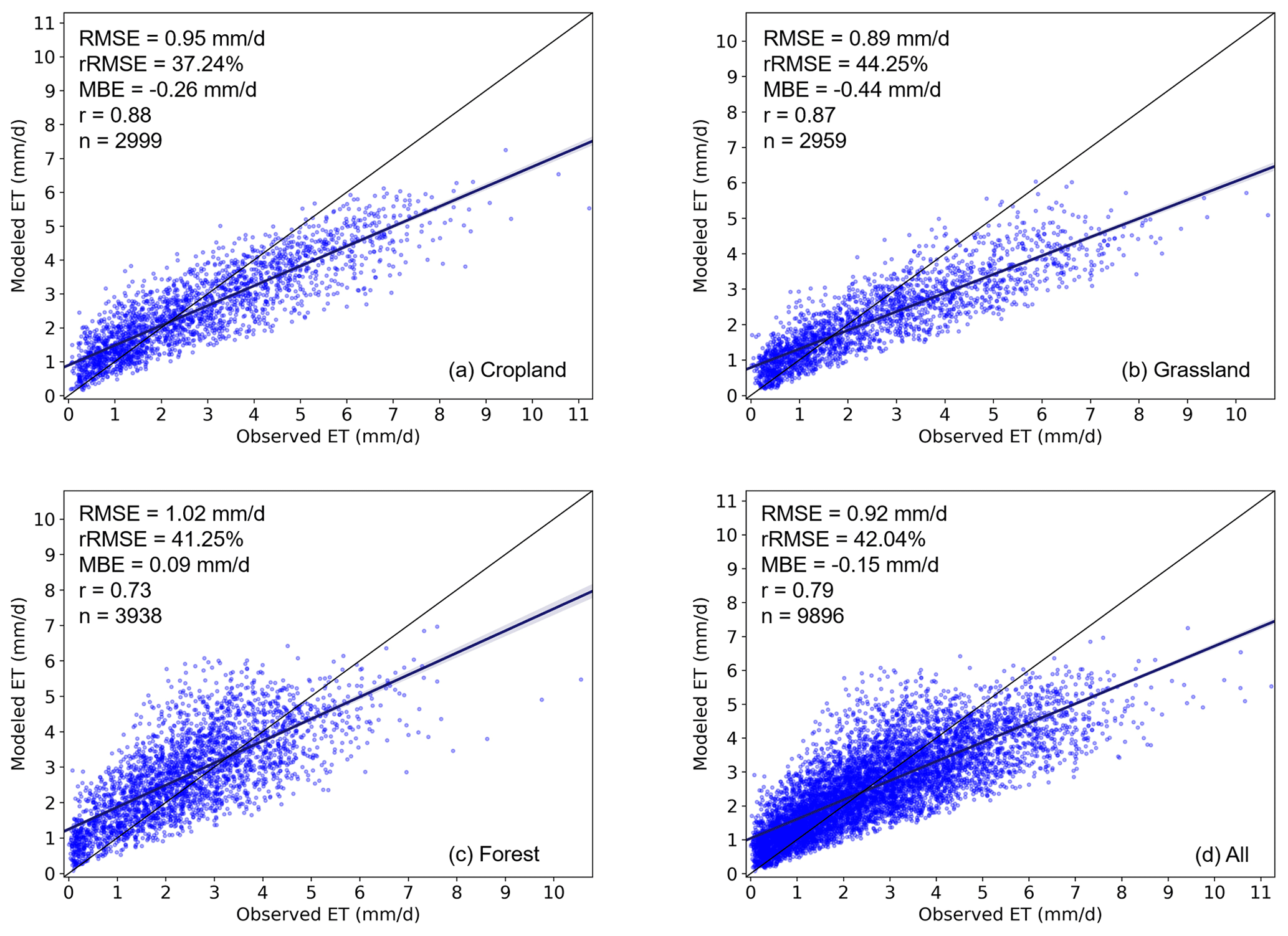
Figure 3 The validation of daily ET estimates using the SEBAL model and multisource images. (a) Cropland; (b) grassland; (c) forest; (d) all land cover types.

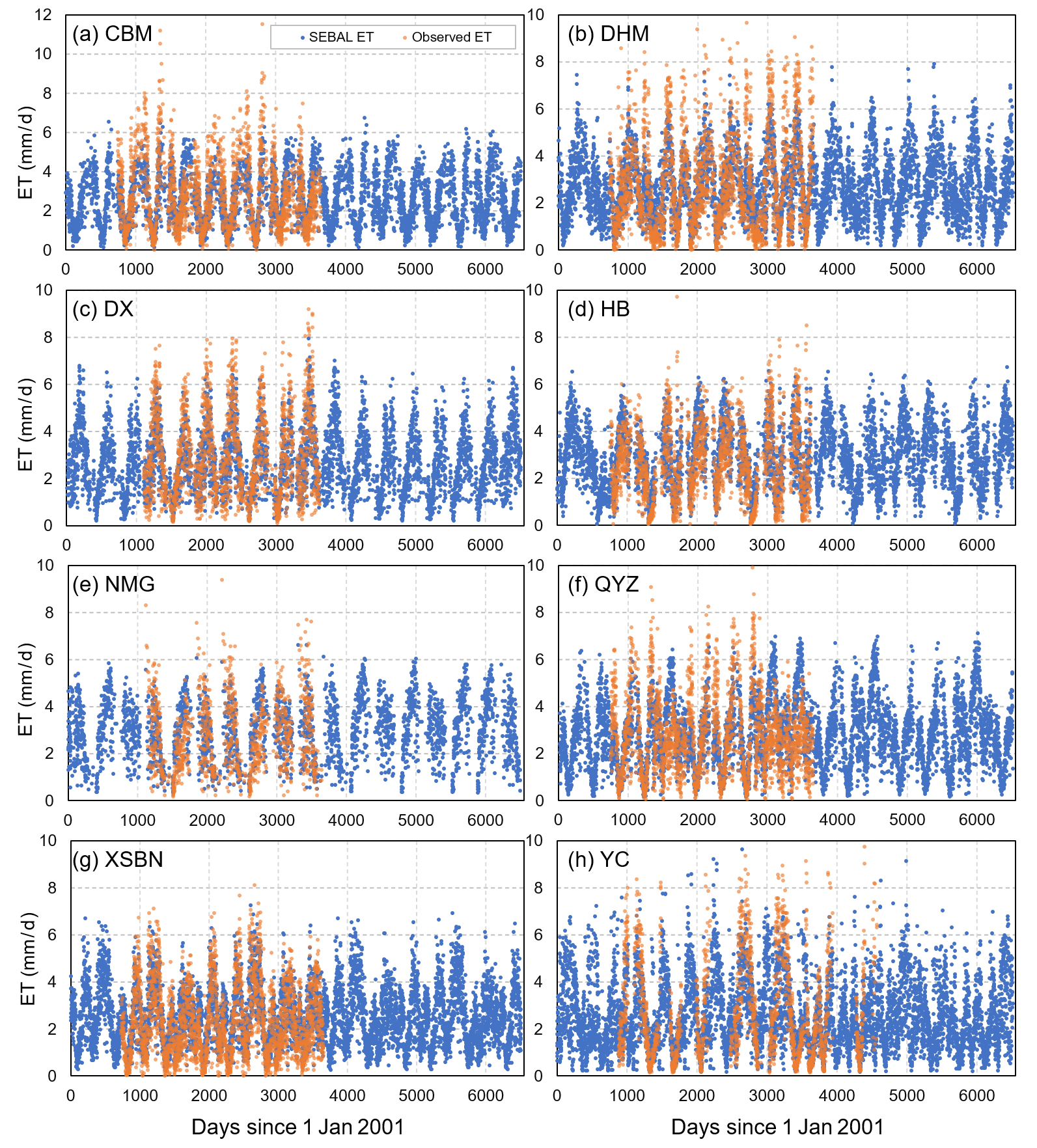
Figure 4 The SEBAL ET and flux-tower-observed ET variation in time series. (a) CBM; (b) DHM; (c) DX; (d) HB; (e) NMG; (f) QYZ; (g) XSBN; (h) YC.

3 Results

3.1 Validation of daily SEBAL ET at the point scale using flux tower observations

The validation results for the daily SEBAL ET (ET_SEBAL) obtained using flux tower observational data are shown in Fig. 3. Compared to ET_flux, ET_SEBAL showed a good performance in China; the two data types showed high consistency, with an r value of 0.79 with 9896 samples. However, the bias of SEBAL was relatively high; the RMSE and rRMSE were 0.92 mm d⁻¹ and 42.04 %, respectively. As shown in the scatter diagrams in Fig. 3, ET_SEBAL showed a negative bias at high values and a positive bias at low values. In general, SEBAL underestimated ET in China, with an MBE of −0.15 mm d⁻¹. Moreover, the daily ET_SEBAL performed similarly for different land use types. The daily ET_SEBAL had a bias of 0.95 mm d⁻¹ (rRMSE = 37.24 %) in cropland and 0.89 mm d⁻¹ (rRMSE = 44.25 %) in grassland, and the daily ET_SEBAL underestimated in both cropland and grassland, with MBEs of −0.26 mm d⁻¹ and −0.44 mm d⁻¹, respectively. In forest, the daily ET_SEBAL had the highest RMSE of 1.02 mm d⁻¹ (rRMSE = 41.25 %) and the lowest r value of 0.73, and it was slightly overestimated compared to ET_flux (MBE = 0.09 mm d⁻¹). Figure 4 shows the time series variation of ET. In general, SEBAL ET and observed ET both showed a clear seasonal variation characteristic among the eight flux tower stations. Moreover, an annual periodic variation was found at most stations (Fig. 4a–e and g). The cropland stations (YC and QYZ) presented a relatively disordered period (Fig. 4g and h), which likely contributed to the double-crop rotation system used in these regions. For example, at the YC station located in the North China Plain, there was generally maize and wheat rotation, which may cause two peaks of crop water consumption (ET) to occur in 1 year. Furthermore, Figs. 3 and 4 both show that SEBAL ET was clearly underestimated at higher ET rates. The observed ET fluctuated higher than SEBAL ET at all stations as shown in Fig. 4.

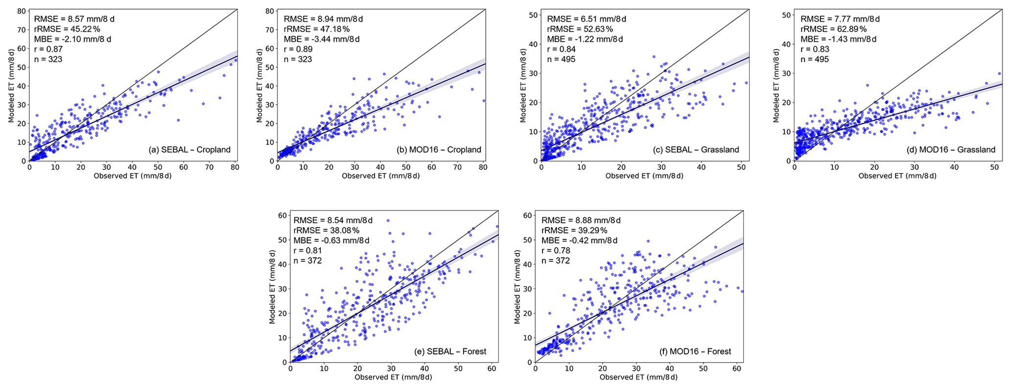
Figure 5 Validations for different land cover types. (a) SEBAL ET for cropland; (b) MOD16 ET for cropland; (c) SEBAL ET for grassland; (d) MOD16 ET for grassland; (e) SEBAL ET for forest; (f) MOD16 ET for forest.

3.2 Comparison of SEBAL and MOD16 ET under different environmental conditions at the 8 d scale

3.2.1 Performance of the RS-based model for different land cover types

The validation results for different land cover types are shown in Fig. 5. The results indicate that the accuracy of SEBAL and MOD16 both varied with land cover type. The RMSE of SEBAL varied from 6.51 to 8.57 mm per 8 d; its rRMSE varied from 38.08 to 52.63 %, and its r value varied from 0.81 to 0.87. The performance of SEBAL was superior for forest (RMSE = 8.54 mm per 8 d, rRMSE = 38.08 %) compared to other land cover types, and the lowest accuracy was obtained over grassland (RMSE = 6.51 mm per 8 d, rRMSE = 52.63 %). The results of the MOD16 validation indicate that MOD16 had a better performance for forest (RMSE = 8.88 mm per 8 d, rRMSE = 39.29 %) than other land cover types, as was observed for SEBAL, and the performance of MOD16 over grassland was also the worst (RMSE = 7.77 mm per 8 d, rRMSE = 62.89 %). The MBE values for MOD16 varied from 0.42 to 3.44 mm per 8 d, which indicates that both the ET models underestimated ET over all land cover types. Overall, the accuracy of SEBAL was higher than that of MOD16.

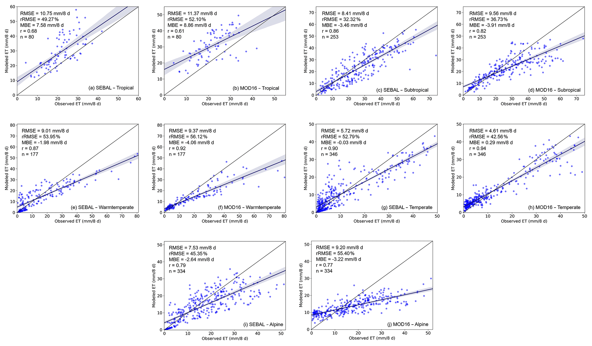
Figure 6 Validations for different climate zones. (a) SEBAL ET for tropical zones; (b) MOD16 ET for tropical zones; (c) SEBAL ET for subtropical zones; (d) MOD16 ET for subtropical zones; (e) SEBAL ET for warm–temperate zones; (f) MOD16 ET for warm–temperate zones; (g) SEBAL ET for temperate zones; (h) MOD16 ET for temperate zones; (i) SEBAL ET for alpine zones; (j) MOD16 ET for alpine zones.

3.2.2 Performance of the RS-based model for different climate zones

The validation results for different climate zones are shown in Fig. 6. The results show that the r value varied from 0.68 to 0.90 for SEBAL and varied from 0.61 to 0.94 for MOD16. Climate zones were found to influence the accuracy of the RS-based models. In tropical zones, both models showed poor accuracy, with RMSEs of 10.75 and 11.37 mm per 8 d for SEBAL and MOD16, respectively, and low r values of 0.68 and 0.61 for SEBAL and MOD16, respectively. Additionally, both the models overestimated, with MBEs of 7.58 and 8.86 mm per 8 d for SEBAL and MOD16, respectively. For subtropical zones, both the models had high precision, with rRMSEs of 32.32 % and 36.73 % for SEBAL and MOD16, respectively, and both underestimated, with r values of 0.86 and 0.82 for SEBAL and MOD16, respectively. For warm–temperate zones, both SEBAL and MOD16 showed poor accuracy, with rRMSEs of 53.95 % and 56.12 %, respectively, and both underestimated. For temperate zones, MOD16 overestimated, while SEBAL underestimated, and both models had high r values, namely 0.90 for SEBAL and 0.94 for MOD16, and low RMSEs of 5.72 mm per 8 d for SEBAL and 4.61 mm per 8 d for MOD16. In general, MOD16 performed better than SEBAL for temperate zones. For alpine zones with low temperature, both the models still underestimated; however, SEBAL performed better than MOD16: the RMSE was 7.53 and 9.20 mm per 8 d, and the r value was 0.79 and 0.77 for SEBAL and MOD16, respectively.

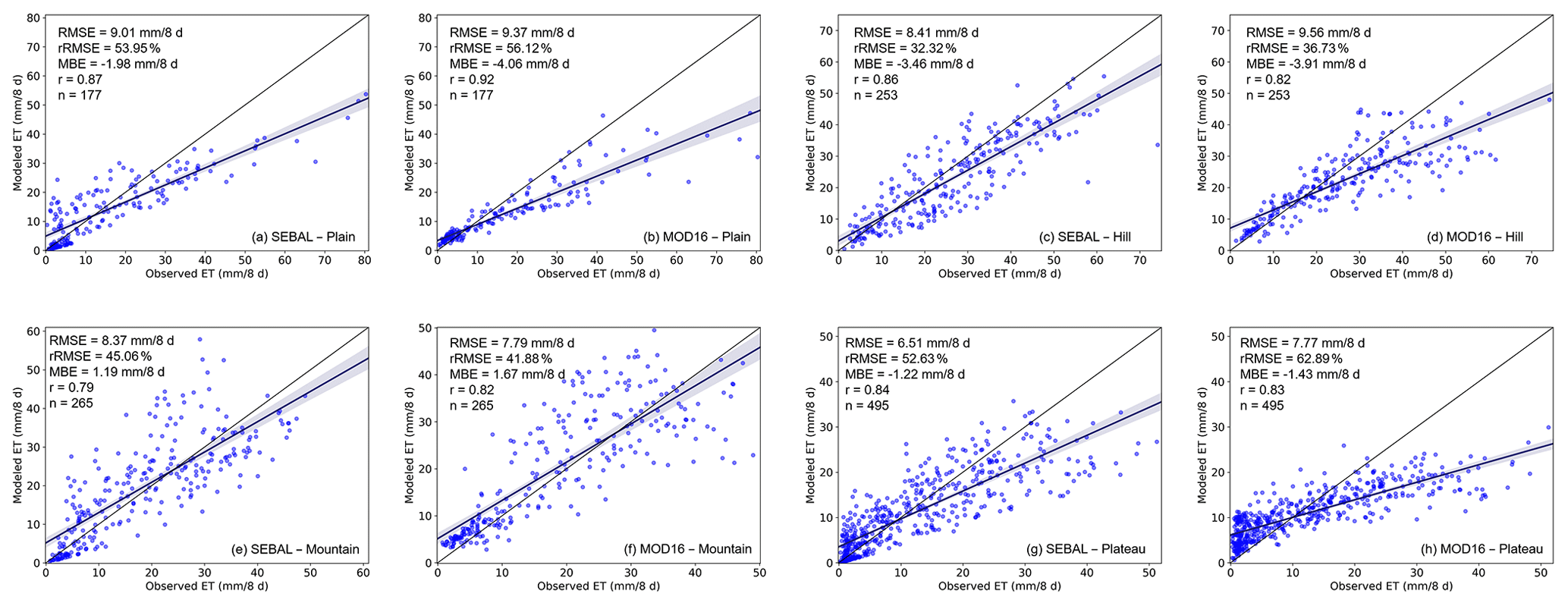
Figure 7 Validation over different terrain: (a) SEBAL ET in plain area; (b) MOD16 ET in plain area; (c) SEBAL ET in hill area; (d) MOD16 ET in hill area; (e) SEBAL ET in mountain area; (f) MOD16 ET in mountain area; (g) SEBAL ET in plateau area; (h) MOD16 ET in plateau area.

3.2.3 Performance of the RS-based model over different terrain types

The validation results for different terrain types are shown in Fig. 7. The results indicate that both models showed a negative bias (negative MBE) for all terrain types except mountainous areas, for which both models overestimated, with MBEs of 1.19 and 1.67 mm per 8 d for SEBAL and MOD16, respectively. In general, for mountainous areas, MOD16 showed a higher accuracy (RMSE = 7.79 mm per 8 d, rRMSE = 41.88 %, r = 0.82) than SEBAL (RMSE = 8.37 mm per 8 d, rRMSE = 45.06 %, r = 0.79). However, for all other terrain types, SEBAL showed a higher accuracy. With SEBAL, the RMSE decreased from 9.01 to 6.51 mm per 8 d as elevation increased. For hilly areas, SEBAL showed the lowest rRMSE (32.32 %), while MOD16 showed the highest rRMSE (36.73 %). For plain areas, SEBAL showed a slightly higher accuracy (RMSE = 9.01 mm per 8 d, rRMSE = 53.95 %) than MOD16 (RMSE = 9.37 mm per 8 d, rRMSE = 56.12 %), while for plateau area, SEBAL (RMSE = 6.51 mm per 8 d, rRMSE = 52.63 %) was more accurate than MOD16 (RMSE = 7.77 mm per 8 d, rRMSE = 62.89 %).

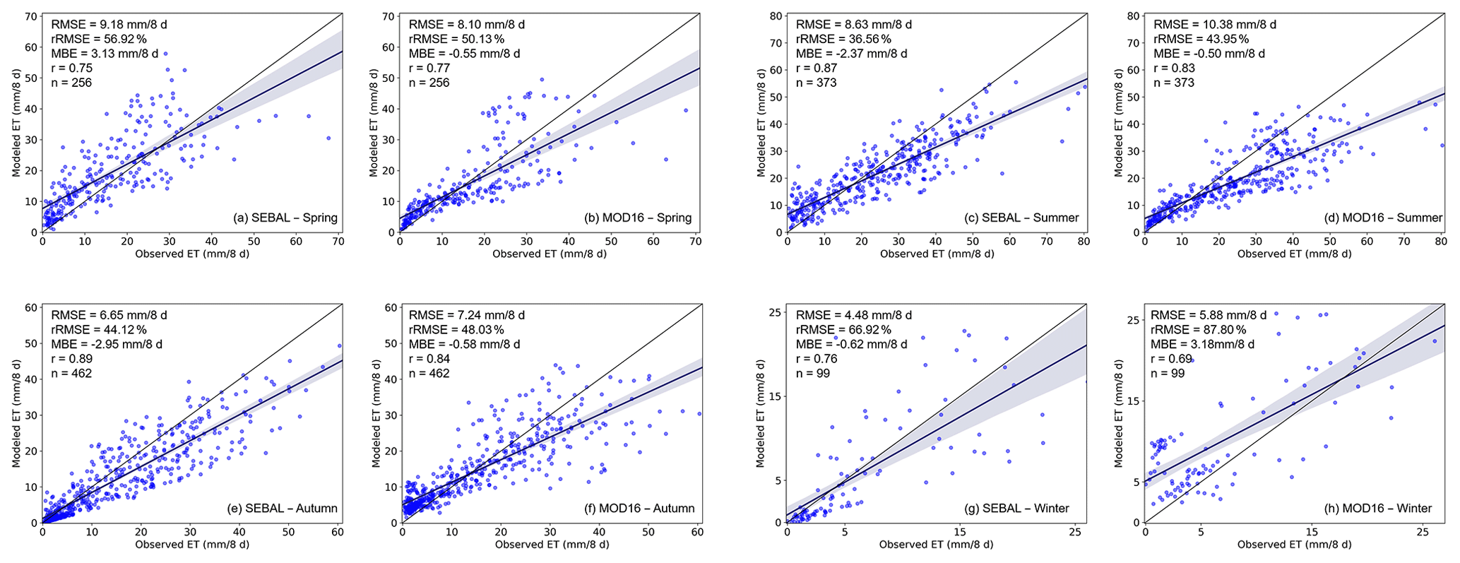
Figure 8 Validation for different seasons. (a) SEBAL ET for spring; (b) MOD16 ET for spring; (c) SEBAL ET for summer; (d) MOD16 ET for summer; (e) SEBAL ET for autumn; (f) MOD16 ET for autumn; (g) SEBAL ET for winter; (h) MOD16 ET for winter.

3.2.4 Performance of the RS-based model in different seasons

The validation results for different seasons are shown in Fig. 8. SEBAL showed a negative bias in summer, autumn, and winter, with MBE values varying from −2.95 to −0.62 mm per 8 d, and showed a positive bias in spring (MBE = 3.13 mm per 8 d). MOD16 showed a positive bias in winter (MBE = 3.8 mm per 8 d) and a negative bias in other seasons, with MBE values varying from −0.58 to −0.50 mm per 8 d. In spring, MOD16 generally showed a better performance (RMSE = 8.10 mm per 8 d, rRMSE = 50.13 % and r = 0.77) than SEBAL (RMSE = 9.18 mm per 8 d, rRMSE = 56.92 % and r = 0.75), while SEBAL performed better than MOD16 in other seasons. In winter, both the models showed a poor performance, with rRMSEs of 66.92 % and 87.80 % for SEBAL and MOD16, respectively. For both models, the highest accuracy was achieved in summer, with rRMSEs of 36.56 % and 43.95 % for SEBAL and MOD16, respectively. Meanwhile, the highest r values were obtained in autumn, with values of 0.89 and 0.84 for SEBAL and MOD16, respectively.

Figure 9 The results of the overall validation. (a) SEBAL ET validation at the 8 d scale; (b) MOD16 ET validation at the 8 d scale.

3.2.5 Summary of point-scale validation

Based on the contents of Sect. 3.1.1–3.1.4, SEBAL showed a higher accuracy than MOD16 in most conditions, while MOD16 showed a better performance only for temperate zones, mountainous areas, and the spring season based on the values of RMSE and rRMSE. Moreover, both the models underestimated for all conditions, except SEBAL overestimated for tropical zones (MBE = 7.58 mm per 8 d), mountainous areas (MBE = 1.19 mm per 8 d), and spring (MBE = 3.13 mm per 8 d), and MOD16 overestimated for tropical zones (MBE = 8.86 mm per 8 d), temperate zones (MBE = 0.29 mm per 8 d), mountainous areas (MBE = 1.67 mm per 8 d), and winter (MBE = 3.18 mm per 8 d). In general, SEBAL showed a higher accuracy than MOD16 based on point-scale validation (Fig. 9). For SEBAL and MOD16, respectively, the RMSE was 7.77 and 8.43 mm per 8 d, the rRMSE was 44.91 % and 48.72 %, and the r value was 0.85 and 0.83. Furthermore, both the models slightly underestimated overall, with an MBE of −1.27 and −1.66 mm per 8 d for SEBAL and MOD16, respectively.

Table 2 The performance of the ET estimation of RS-based models at the basin scale.

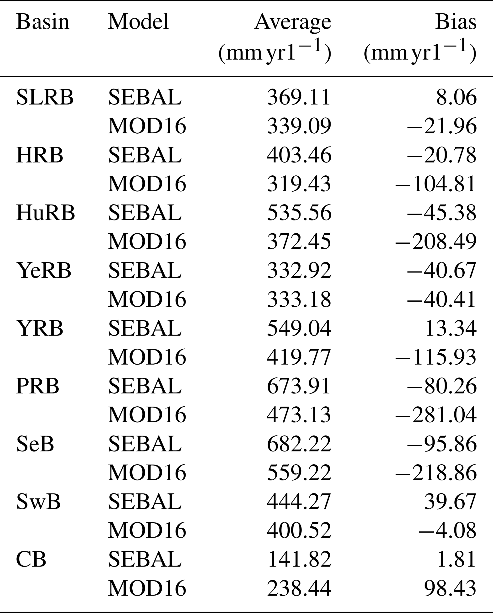
SwB: Southwest Basin; CB: Continental Basin; PRB: Pearl River Basin; YRB: Yangtze River Basin; SeB: Southeast Basin; HRB: Haihe River Basin; YeRB: Yellow River Basin; HuRB: Huaihe River Basin; SLRB: Songhua and Liaohe River Basin.

Figure 10 The results of validation at the basin scale.

3.3 Validation at the basin scale using the water balance method

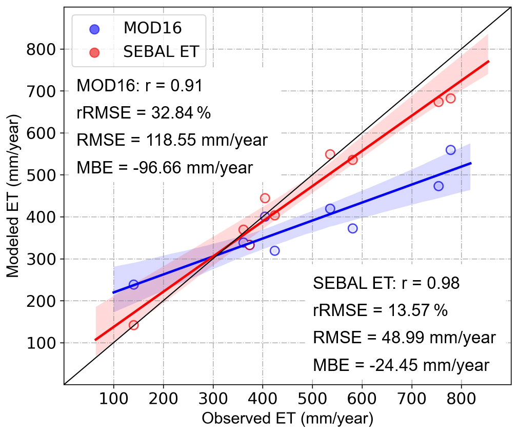
Additionally, validation using hydrological data was performed to investigate the performance of the RS-based models at the basin scale. The results (Fig. 10) show that both the models had a negative bias, with an MBE of −24.45 and −96.66 mm yr⁻¹ for SEBAL and MOD16, respectively, at the basin scale. SEBAL showed a higher accuracy, with an RMSE of 42.05 mm yr⁻¹, an rRMSE of 12.65 %, and an r value of 0.98 (MOD16: RMSE = 118.55 mm yr⁻¹, rRMSE = 32.84 %, r = 0.91). As shown in Table 2, the average ET of SEBAL varied from 141.83 to 682.22 mm yr⁻¹ among the different basins, while bias varied from −95.86 to 39.67 mm yr⁻¹. The average ET of MOD16 varied from 238.44 to 559.22 mm yr⁻¹ among the different basins, while bias varied from −281.04 to 98.43 mm yr⁻¹.

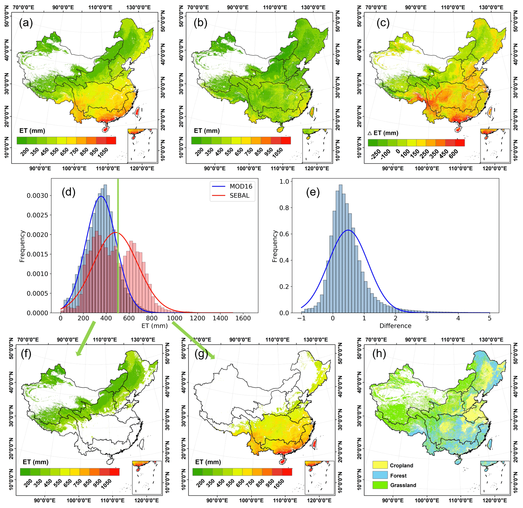
Figure 11 A comparison between the SEBAL and MOD16 models. (a) Distribution of annual average ET_SEBAL. (b) Distribution of annual average ET_MOD. (c) Distribution of the difference between SEBAL and MOD16 (ETSEBAL – ETMOD). (d) Histogram of annual average ET_SEBAL and ET_MOD. (e) Histogram of the relative difference between SEBAL and MOD16 ((ET_SEBAL – ET_MOD)/ET_MOD). (f) Map of ET_SEBAL below 500 mm. (g) Map of ET_SEBAL over 500 mm. (h) Land cover in China.

3.4 Comparison of the spatial distribution of ET between SEBAL and MOD16

Regarding the modeled spatial distribution of ET, both the SEBAL and MOD16 models showed that the annual average (2001–2018) ET in China increased from the northwest to the southeast (Fig. 11a, b, and d). The annual ET of SEBAL varied from 0 to 1600 mm in space, with a mean value of 482.27 ± 192.31 mm, while that of MOD16 varied from 0 to 1200 mm, with a mean value of 359.61 ± 59.52 mm. In general, compared to the ET value estimated using MOD16 and SEBAL, the ET value estimated using SEBAL was higher and showed a greater spatial difference of ET in China. For 84.07 % of the total area of China, the annual ET estimated by SEBAL was higher than that estimated by MOD16; for 14.07 % of the total area of China, the difference was more than 2 times – these areas are mainly distributed in southern China, where ET is relatively high, and the difference reaches more than 600 mm in some places. Only in 15.93 % of the total area of the country was the annual ET estimated by SEBAL lower than that estimated by MOD16; these areas are mainly distributed in northwestern China, where ET is relatively low (Fig. 11c and e). Regarding the distribution of ET_SEBAL, a bimodal curve with the boundary of ∼ 500 mm is shown in Fig. 11d; it was likely contributed by the misestimation of parts of regions. The ET_SEBAL map was divided into two parts with 500 mm as a threshold value; the part of ET_SEBAL below 500 mm was distributed in northwestern China (Fig. 11f), whereas the part of ET_SEBAL over 500 mm was distributed in the southeast (Fig. 11g). It should be noted that the vegetation cover in the northwest of China is mainly grassland and a small fraction of cropland (Fig. 11h), and the ET_SEBAL of grassland and cropland was underestimated by the SEBAL model (Sect. 3.1). In contrast, the ET_SEBAL showed slightly overestimated forest, which is the main land cover type in the southeast of China. Therefore, the distributed ET_SEBAL around ∼ 500 mm was underestimated or overestimated and thus formed the bimodal curve.

4 Discussion

4.1 Summary of validation results and comparison with other studies

The ET_SEBAL showed a relatively good performance in China as a whole, with an average r value of 0.79 and an average RMSE of 0.92 mm d⁻¹. These results are close to those obtained in other studies. Rahimzadegan and Janani (2019) used SEBAL to estimate the actual ET of pistachio in Semnan, Iran, and found that the modeled value had a high consistency with the in situ measured value (r = 0.80); this value was slightly lower than the cropland validation obtained in the present study (r = 0.88, daily scale). This difference is mainly due to differences in the validation method between these two studies. Rahimzadegan and Janani (2019) used the P–M equation and field observational data from intelligent meteorological instruments to measure the standard ET, and MOD16 data, which are also based on the P–M equation, were evaluated in this study as performing worse than the SEBAL estimation at both point scale and basin scale. Xue et al. (2020) used pySEBAL (SEBAL in the Python environment) to estimate the ET of almonds, tomatoes, and maize in the Central Valley of California, USA, and showed that the r value and RMSE of pySEBAL varied from 0.60 to 0.86 and from 1.08 to 1.79 mm d⁻¹, respectively; the authors used Landsat 8 OLI/TIRS images with a spatial resolution of 30 m × 30 m as the model input, which leads to a lower influence of mixed pixels compared to MODIS data with a spatial resolution of 1 km × 1 km. Wagle et al. (2017) evaluated the performance of SEBAL for ET estimation for sorghum based on flux tower observational data from Oklahoma, USA; the results showed that the r value varied from 0.73 to 0.87, while the RMSE varied from 0.83 to 1.24 mm d⁻¹, which is basically in agreement with the results of this study (r value varied from 0.68 to 0.90 and RMSE varied from 4.48 to 10.75 mm per 8 d under different environmental conditions). MOD16 performed worse than SEBAL. Part of the bias is caused by objective factors such as the inaccuracy of the input data and the limitations of the validation methods. Meanwhile, additional bias is contributed by the subjective factor of the innate defects of the algorithms. These factors will be discussed in detail in Sects. 4.2 and 4.3. Overall, the SEBAL ET showed an acceptable performance in China as demonstrated by comparing pervious studies.

4.2 Errors caused by objective factors

4.2.1 Inaccuracy of input data

Both SEBAL and MOD16 used MODIS data as the main input images (e.g., MCD43 surface albedo, MOD13 NDVI, MOD11 surface temperature). However, the accuracy of these data is uncertain to some extent (Ramoelo et al., 2014). For instance, surface albedo is a critical radiative parameter; however, complex algorithm-led remote-sensing-based albedo products can contain errors introduced by the spectral conversion (Song et al., 2020). Wang et al. (2014) compared MODIS albedo products with ground data and Landsat data for different land cover types in the USA and found that the RMSE of the products varied from 0.01–0.05 and that the error was higher during periods of snow cover. Furthermore, surface temperature, as a fundamental parameter for the calculation of surface energy balance, affected the estimation of ET to a great extent (Long et al., 2011). Timmermans et al. (2006) analyzed the sensitivity of each parameter of the SEBAL model to grassland in Oklahoma, USA, and the results indicated that the difference in surface air temperature had the greatest influence on the accuracy of SEBAL estimation. MODIS surface temperature products are retrieved using the split-window algorithm. Yu et al. (2019) used in situ measurement data to validate MODIS surface temperature products in the Heihe River Basin (HRB) in northwestern China; the results indicated that the daytime MOD11 (obtained by the Terra satellite) and MYD11 (obtained by the Aqua satellite) products have accuracies of −0.84 ± 0.88 K and −0.11 ± 0.42 K, respectively. In general, original MODIS data contained errors to some extent.

Additionally, gap filling of missing or unreliable MODIS data may cause the errors to some extent. For example, spring and summer have relatively frequent precipitation, which causes more unreliable pixels due to clouds, and these pixel values were finally replaced by gap filling the nearest date pixel value; therefore, the modeled ET value of these pixels was close to that of the nearest date without precipitation. In fact, due to the high air humidity on rainy days, evaporation and transpiration are relatively less than that of the nearest date (Ferreira and Cunha, 2020; Li et al., 2016). Moreover, it should be noted that due to the decrease in surface available radiation energy caused by cloud cover, the ET (both the actual and modeled value) is also less than that of the nearest date (Cheng et al., 2020). This may explain the obvious overestimation at lower ET rates in spring, summer, and other pixels affected by cloud. Furthermore, a relatively high bias of SEBAL ET was found in winter; the rRMSE reached 66.92 % (the highest value among all situations). Ice and snow cover caused by frequent snowfall and low temperature in winter, which will affect remotely sensed information to a great extent, e.g., reflectance (Casey et al., 2017), will further affect the ET estimation. Moreover, the underestimation was found at higher ET rates in most situations as shown in Figs. 4–10, which may be caused by the saturation issue of optical sensors (Maimaitijiang et al., 2020). For example, under dense vegetation cover, the vegetation index (e.g., NDVI) was likely underestimated and cannot accurately characterize vegetation status (Maimaitijiang et al., 2020; Vergara-Díaz et al., 2016); therefore, soil heat flux will be overestimated (Eq. A9 in Appendix A) and may further cause the latent heat flux underestimation.

4.2.2 Errors in flux tower measurements

The eddy covariance system (flux tower observations) is the most commonly used observation system to calculate and analyze the energy and mass exchange between the surface and atmosphere (Wang and Dickinson, 2012). However, the typical error of ET estimation based on the eddy covariance system is about 5 %–20 % (Culf et al., 2008; Vickers et al., 2010). Also, the eddy covariance system generally has an energy balance non-closure issue: the sum of the soil heat flux, sensible heat flux, and latent heat flux was found to be less than net radiation in most cases (Mu et al., 2011; Wilson et al., 2002). Recently, it was found that the non-closure issue of the energy balance was explained by the energy fluxes from secondary circulations and larger eddies that cannot be captured by EC measurement at a single station (Foken et al., 2011). In this study, the Bowen ratio method (Eq. 3), which assumes that the residual of the energy balance is attributed to sensible and latent heat flux and assigns the missing energy flux to them (Song et al., 2016; Wang et al., 2019), was used to enforce energy closure. Actually, this assumption is not very correct, which generally led to sensible and latent heat flux overestimation (Song et al., 2016); this could explain why the SEBAL ET was generally underestimated when compared to flux-tower-observed ET (Fig. 9). The same issue was found in regional-scale validation due to the ignoring of ΔS in the water balance computation process (although small), which could lead to the regional ET overestimation and further cause SEBAL ET underestimation in regional validation (Fig. 10).

Additionally, the mismatch of the flux tower footprint and spatial resolution of SEBAL ET will causes errors as well. Generally, the footprint of the flux tower varied from hundreds of square meters to several square kilometers, which was determined by the height of the observation instrument, the intensity of the turbulence, terrain, environment, and vegetation status (Chen et al., 2012; Damm et al., 2020; Schmid, 1994). Moreover, a footprint probability distribution function (PDF) could characterize the footprint at a fine spatial resolution (Wang et al., 2019), but it may not be suitable for the coarse resolution in this study (kilometer scale). In this study, the 1 km × 1 km area of the pixel was used for matching the footprint of the flux tower, which refers to the study of Velpuri et al. (2013); however, the footprint is not stable but varies with environmental change, e.g., vegetation height. Chen et al. (2012) reported that the forest footprint has a clear difference with grassland; the footprint of forest is much larger, which reaches the kilometer scale. In fact, the forest footprint may match the spatial resolution better in this study. Therefore, it may explain why the SEBAL ET has the greatest performance in forest but the worst performance in grassland. Compared to the study of Velpuri et al. (2013), the grassland also showed the worst remote sensing ET estimation in the US when using flux tower data for validation at a kilometer scale.

Although a comprehensive evaluation of SEBAL ET over different classes was conducted in this study, users should be aware of the uncertainties due to the limited number of validation sites in some classes. For example, only one site was available for the evaluation over cropland. Because this cropland flux tower site was set in a plain and warm–temperate zone, the accuracy may only represent the data quality of cropland ET in the warm–temperate plain zone, but not other regions. Nevertheless, long-time-series data were obtained from this site, which covered different seasons and different crop types. Employing these hundreds of samples in the validation could remedy the single-site insufficiency to a certain extent. Similarly, only one site was found in the validation over two other classes, i.e., the tropical zone and warm–temperate zone. Long-time-series data were also incorporated to enhance the representativeness of the single site. Regarding the other classes, two or more sites were used, which will lead to more reliable results. Compared to previous studies (Aguilar et al., 2018; Hu et al., 2015; Ramoelo et al., 2014; Yang et al., 2017), a larger number of validation samples (flux tower sites) were used in this study, indicating that the findings are reliable. Additionally, although the validation of SEBAL ET in this study followed the literature (Kim et al., 2012; Ramoelo et al., 2014) and considered different land cover types, climate zones, elevation, and seasons, several more situations may need to be considered: for example, whether the SEBAL accuracy was different across years (Velpuri et al., 2013) and satellite sensors (Long et al., 2011). Overall, with the increasing number of flux towers set up in China, more reliable and comprehensive validation of SEBAL ET can be conducted in follow-up research.

4.3 Errors caused by subjective factors

4.3.1 Temporal scaling-up method

Remotely sensed information represents the satellite-passing time. Therefore, in the RS-based models, scaling up was performed from the instantaneous level to the daily level. SEBAL uses the evaporative fraction (Λ) for scaling up (Gao et al., 2020), as shown in Eqs. (A30) and (A31). However, several studies have indicated that the assumption of a constant evaporative fraction is not very reasonable (Gentine et al., 2011; Hoedjes et al., 2008). Gentine et al. (2007) proposed that soil moisture and vegetation resistance are the factors that mainly affect the stability of Λ, and soil moisture is positively correlated with Λ. Additionally, a larger leaf area index will generally lead to a lower stability of Λ under the same soil moisture (Farah et al., 2004). In general, due to the instability of Λ, the above assumption will cause a negative bias of 10 %–20 % in the estimation of daily ET (Delogu et al., 2012; Ryu et al., 2012; Van Niel et al., 2012). This can explain why the validation in this paper showed that the ET estimated using SEBAL was underestimated. While the MOD16 model estimates daily ET using the P–M equation, which is a semi-empirical equation, it uses 8 or 16 d composite remotely sensed input data and daily meteorological input data to compute the 8 d composite ET products (Mu et al., 2011). The use of a semi-empirical equation avoids the need to perform scaling up; however, it has the problem of theoretical deficiency (Mu et al., 2007; Ramoelo et al., 2014).

4.3.2 Calculation of sensible heat flux

Sensible heat flux is the most complicated part of the energy balance calculation (Wang and Dickinson, 2012). The P–M algorithm defines the available energy (A, unit: W m⁻²) as the sum of the sensible heat flux and latent heat flux (Eq. 10) (Mu et al., 2011).

$$\begin{array}{}\text{(10)}& A=H+\mathit{\lambda }\text{ET}=R_{\mathrm{n}}-G\end{array}$$

The P–M algorithm calculates λET using a semi-empirical formula and A, and it therefore avoids the direct calculation of H. Meanwhile, SEBAL calculates H based on MOST and the hot–cold pixel (Bastiaanssen et al., 1998a, b). However, several studies have indicated that MOST has an error of 10 %–20 % for the estimation of the boundary layer thickness (Foken, 2006; Högström and Bergström, 1996). Therefore, MOST is also a source of error in SEBAL. Due to the complexity of the sensible heat flux, SEBAL makes several assumptions to estimate H, which may introduce error into the ET estimation (Zheng et al., 2016).

Figure 12 The performance of different domain sizes used in SEBAL ET estimates.

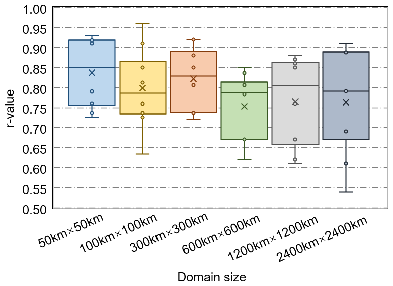
Additionally, the selection of the hot–cold pixel depends on the domain size (the actual size of the modeling domain and/or satellite imagery being used). For instance, the basin-scale selection of the hot–cold pixel with diverse vegetation cover and single vegetation cover, respectively, will lead to different results for dT. Theoretically, with the domain size increasing, there is a possible tendency of T_{s_hot} increasing and T_{s_cold} decreasing. For example, if T_{s_cold} remains invariant and T_{s_hot} increases under the condition of domain size increasing, the H estimates will decrease and λET estimates could thus increase. In the study of Long et al. (2011), the results showed that a 2 K increase in T_{s_hot} will result in a 9.3 % increase but a 9.1 % decrease in a and b, respectively, and further caused an 11.8 % mean decrease in H. Recently, the study of Saboori et al. (2021) reported that the cold pixel performed more stably than the hot pixel in time series, especially in winter; the hot pixel being highly varied may be due to the similarity of NDVI over space, and it could further explain the poor performance of SEBAL ET in winter. Seguin et al. (1999) demonstrated that the method of hot–cold pixel selection for the estimation of H generally has an accuracy of ∼ 50 W m⁻². In this study, the ET was computed in the domain size of 1200 km × 1200 km, which is a relatively large area. The performances of different domain sizes in ET computation were compared (Fig. 12) and resulted in generally better performance in smaller areas, which may be due to the relatively limited spatial heterogeneity (Long et al., 2011). However, a larger domain size may have faster computational efficiency of ET on a regional scale. The trade-off between efficiency and accuracy (i.e., most suitable domain size) needs to be further studied. Overall, the domain size employed in this study (1200 km × 1200 km) showed acceptable accuracy. Although several algorithms have been proposed that use other methods to avoid the error caused by the selection of the hot–cold pixel, such as the SEBS (Su, 1999), these replaced the selection of the hot–cold pixel with the fitting of dry and wet edges. However, no evidence has been found that the method of fitting dry and wet edges can significantly improve the accuracy of ET estimation (Wagle et al., 2017; Xue et al., 2020).

Besides sensible heat flux, the errors of SEBAL ET may be derived from net radiation or soil heat flux as well (Li et al., 2017; Teixeira et al., 2009). For net radiation, which is computed using surface albedo and the Stefan–Boltzmann law (Eq. A2), there was general agreement with the flux-tower-observed value, while soil heat flux, which is computed using an empirical formula related to net radiation and NDVI (Eq. A9), has a poor performance (Li et al., 2017; Song et al., 2016). In the study of Li et al. (2017), soil heat flux estimation showed a clear overestimation in higher ET areas, e.g., wetland, which may further cause the sensible and latent heat flux underestimation in higher ET rates. In most SEBR-based algorithms, similar net radiation and soil heat flux estimation methods are used, and various sensible heat flux estimation methods are the main sources of the difference among the various SEBR-based algorithms. However, the causes of the net radiation and soil heat flux estimation errors have not been clearly discussed, e.g., the effect of satellite transmitted time or land cover types. These issues could be the focus of our follow-up research; for example, geostationary satellites and flux towers with high-frequency observations may be helpful for this research.

5 Data availability

The dataset that was generated using SEBAL with a spatial resolution of 1 km and a temporal resolution of 1 d can be used for various types of geoscientific studies, especially for global change, water resources management, and agricultural drought monitoring. The evapotranspiration (ET) dataset for China is distributed under a Creative Commons Attribution 4.0 international license. The dataset is named SEBAL evapotranspiration in China (SEBAL ET) and consists of 18 years of data. More information and data are freely available from the Zenodo repository at https://doi.org/10.5281/zenodo.4243988 and https://doi.org/10.5281/zenodo.4896147 (Cheng, 2020a, b).

6 Conclusions

In this study, we generated a long-time-series (2001–2018) ET product based on SEBAL and multisource images. We further conducted a comprehensive validation of the product and compared its performance under different environmental conditions in China with the performance of the ET estimated using MOD16 data. The conclusions are as follows.

1. The ET product generated using SEBAL showed a good performance in China. Compared to flux tower observational data, the r value of the SEBAL ET reached 0.79 for 9896 samples; the RMSE was 0.92 mm d⁻¹ and the rRMSE was 42.04 %. SEBAL underestimated ET as a whole, with an MBE of −0.15 mm d⁻¹. The SEBAL ET product can adequately represent the actual ET and can be used in research on water resources management, drought monitoring, and ecological change, for example.

2. Based on observational data from eight flux towers from 2003 to 2010, the ET datasets estimated using SEBAL and MOD16 were validated at the 8 d scale for different land cover types, climate zones, terrain types, and seasons. The results showed that SEBAL performed best in the conditions of forest cover (rRMSE = 38.08 %), subtropical zones (rRMSE = 32.32 %), hilly terrain (rRMSE = 32.32 %), and the summer season (rRMSE = 36.56 %) and performed worst in the conditions of grassland cover (rRMSE = 52.63 %), warm–temperate zones (rRMSE = 53.95 %), plain terrain (rRMSE = 53.95 %), and the winter season (rRMSE = 66.92 %). MOD16 performed best in the conditions of forest cover (rRMSE = 39.29 %), subtropical zones (rRMSE = 36.73 %), hilly terrain (rRMSE = 36.73 %), and the summer season (rRMSE = 43.95 %) and performed worst in the conditions of grassland cover (rRMSE = 62.89 %), warm–temperate zones (rRMSE = 52.10 %), plateau terrain (rRMSE = 62.89 %), and the winter season (rRMSE = 87.80 %). In general, the two models have similar adaptability to different conditions, although SEBAL performed slightly better than MOD16.

3. Based on flux tower observational data and hydrological observational data, the ETs estimated by SEBAL and MOD16 were validated at the point scale and basin scale. The results showed that, at the point scale, the accuracy of SEBAL was 7.77 mm per 8 d for the RMSE, 44.91 % for the rRMSE, and 0.85 for the r value; the accuracy of MOD16 was 8.43 mm per 8 d for the RMSE, 48.72 % for the rRMSE, and 0.83 for the r value. At the basin scale, the accuracy of SEBAL was 48.99 mm yr⁻¹ for the RMSE, 13.57 % for the rRMSE, and 0.98 for the r value. In general, SEBAL performed slightly better than MOD16 at the point scale, while SEBAL had a larger accuracy advantage at the basin scale.

4. Overall, the SEBAL ET is higher than the MOD16 ET: for 84.07 % of the total area of China, the SEBAL ET showed higher values. Additionally, the SEBAL ET is closer to the in situ measured ET in most conditions, while the MOD16 ET performed better only in temperate zones, mountain areas, and the spring season. In general, the two models both have a good performance and can be used in the qualitative analysis and most quantitative analyses of regional ET. Furthermore, the combination of the two models can improve the overall ET estimation accuracy for use in applications with higher accuracy requirements.

Compared to the widely used MOD16 ET data, the SEBAL ET product showed a higher accuracy and temporal resolution. However, it still has a daily error of 42.04 % (0.92 mm d⁻¹) at the point scale and a yearly error of 13.57 % (48.99 mm yr⁻¹) at the basin scale. Therefore, the improvement of the SEBAL algorithm will be the focus of follow-up research. Moreover, the 1 km spatial resolution of the SEBAL ET product cannot meet the requirements of more detailed research. Due to the difficulty of simultaneously satisfying the requirements for the spatial and temporal resolutions of remote sensing data, the fusion of multiple sources of remote sensing data may be the most effective way to improve the spatiotemporal resolution of daily ET products.

Appendix A: Description of generating SEBAL ET in detail

The SEBAL model calculates the instantaneous λET of the satellite transit time as a residual based on the surface energy balance equation (Eq. A1) as follows:

$$\begin{array}{}\text{(A1)}& \mathit{\lambda }\text{ET}=R_{\mathrm{n}}-G-H,\end{array}$$

where R_n is the net radiation flux, H is the sensible heat flux, and G is the soil heat flux (the unit of all three parameters is W m⁻²). In this paper, MODIS data (MCD43 surface albedo, MOD11 surface temperature, MOD13 NDVI) and meteorological data (air temperature) from the Global Modeling and Assimilation Office (GMAO) were used as input for surface parameterization (R_n, G, and H). The equations for R_n are shown in Eqs. (A2)–(A5) below:

$$\begin{array}{}\text{(A2)}& R_{\mathrm{n}}=(\mathrm{1}-\mathit{\alpha })R_{\text{s\_down}}+R_{\text{l\_down}}-R_{\text{l\_up}},\end{array}$$

where α is the surface albedo obtained from the MCD43 data, and R_{s_down}, R_{l_up}, and R_{l_down} are the downwelling shortwave radiation, downwelling longwave radiation, and upwelling longwave radiation, respectively (the unit of all three parameters is W m⁻²). R_{s_down} can be calculated using the Julian day (used to estimate the astronomical distance between the sun and earth), elevation (used to estimate atmospheric emissivity), and solar zenith angle at the time of satellite transit. R_{l_up} and R_{l_down} can be calculated using the surface temperature (MOD11), NDVI (MOD13, used to estimate surface emissivity), air temperature (GMAO data), and atmospheric emissivity based on the Stefan–Boltzmann law. The equations for R_{s_down}, R_{l_up}, and R_{l_down} are given in Eqs. (A3)–(A5).

$$\begin{array}{}\text{(A3)}& {\displaystyle }{R}_{\text{s\_down}}={\displaystyle \frac{G_{\text{sc}}\cdot \cos \mathit{\theta }\cdot {\mathit{\tau }}_{\text{sw}}}{d_{\mathrm{r}}^{\mathrm{2}}}}\text{(A4)}& {\displaystyle }{R}_{\text{l\_up}}={\mathit{\epsilon }}_{\mathrm{a}}\mathit{\sigma }{T}_{\mathrm{a}}^{\mathrm{4}}\text{(A5)}& {\displaystyle }{R}_{\text{l\_down}}=\mathit{\epsilon }\mathit{\sigma }{T}_{\mathrm{s}}^{\mathrm{4}}\end{array}$$

Here, G_sc is the solar constant (1376 W m⁻²), θ is the solar zenith angle, τ_sw is the atmospheric transmittance (Eq. A6) (Tasumi, 2000), d_r is the astronomical distance between the sun and earth (Eq. A7) (Bastiaanssen et al., 1998a), ε_a and ε are the atmospheric emissivity (Eq. A8) (Bastiaanssen et al., 1998a) and surface emissivity (obtained from MOD11), respectively, σ is the Stefan–Boltzmann constant (5.67 × 10⁻⁸ $\mathrm{W}{\mathrm{m}}^{-\mathrm{2}}{\mathrm{K}}^{-\mathrm{4}}$), and T_a and T_s are the air temperature (unit: K; obtained from GMAO data) and surface temperature (unit: K, obtained from MOD11), respectively.

$$\begin{array}{}\text{(A6)}& {\displaystyle }{\mathit{\tau }}_{\text{sw}}=\mathrm{0.75}\cdot \mathrm{2}\times {\mathrm{10}}^{-\mathrm{5}}\cdot Z\text{(A7)}& {\displaystyle }{d}_{\mathrm{r}}=\mathrm{1}+\mathrm{0.0167}\sin \left({\displaystyle \frac{\mathrm{2}\mathit{\pi }(J-\mathrm{93.5})}{\mathrm{365}}}\right)\text{(A8)}& {\displaystyle }{\mathit{\epsilon }}_{\mathrm{a}}=\mathrm{1.08}(-\ln {\mathit{\tau }}_{\text{sw}}{)}^{\mathrm{0.265}}\end{array}$$

Here, Z is the elevation obtained from a digital elevation model (DEM) (unit: m) and J is the Julian day. G can be calculated by the following empirical equation (Bastiaanssen et al., 1998a):

$$\begin{array}{}\text{(A9)}& \begin{array}{rl}G=& R_{\mathrm{n}}\cdot {\displaystyle \frac{T_{\mathrm{s}}-\mathrm{273.16}}{\mathit{\alpha }}}\left(\mathrm{0.0032}\cdot {\displaystyle \frac{\mathit{\alpha }}{c}}+\mathrm{0.0032}{\left({\displaystyle \frac{\mathit{\alpha }}{c}}\right)}^{\mathrm{2}}\right)\\ & \cdot (\mathrm{1}-\mathrm{0.978}{\text{NDVI}}^{\mathrm{4}}),\end{array}\end{array}$$

where T_s is the surface temperature (unit: K) and c represents the influence of the satellite transit time on G. The value of c is 0.9 for transmission times before 12:00 LT (local time), 1.0 for transmission times between 12:00 and 14:00 LT, and 1.1 for transmission times between 14:00 and 16:00 LT. H can be calculated as follows:

$$\begin{array}{}\text{(A10)}& H={\displaystyle \frac{{\mathit{\rho }}_{\text{air}}{C}_{\mathrm{p}}\text{dT}}{r_{\mathrm{a}}}},\end{array}$$

where ρ_air (unit: kg m⁻³) is the air density (Eq. A11) (Smith et al., 1991), C_p (unit: $\mathrm{J}(\mathrm{kg}\cdot \mathrm{K}{)}^{-\mathrm{1}}$) is the specific heat of air at constant pressure, dT (unit: K) is the difference between the aerodynamic surface temperature (T_z0 h; unit: K) and the reference height temperature (T_a, unit: K), and r_a is the aerodynamic resistance (unit: s m⁻¹) (Eq. A12).

$$\begin{array}{}\text{(A11)}& {\displaystyle }{\mathit{\rho }}_{\text{air}}=\mathrm{349.635}{\displaystyle \frac{(T_{\mathrm{a}}-\mathrm{0.0065}Z{)}^{\mathrm{5.26}}}{T_{\mathrm{a}}^{\mathrm{6.26}}}}\text{(A12)}& {\displaystyle }{r}_{\mathrm{a}}={\displaystyle \frac{\ln \left(\frac{Z_{\mathrm{2}}}{Z_{\mathrm{1}}}\right)}{k{U}_{\mathrm{f}}}}\end{array}$$

Here, k is the von Karman constant (0.41), U_f is the frictional wind speed (unit: m s⁻¹) (Eq. A13), and Z₁ and Z₂ are 0.01 and 2, respectively:

$$\begin{array}{}\text{(A13)}& U_{\mathrm{f}}={\displaystyle \frac{k{U}_{\mathrm{r}}}{\ln (Z_{\mathrm{r}}/z_{\text{0\hspace{0.17em}m}})}},\end{array}$$

where U_r is the wind speed at height Z_r, which can be calculated from the wind speed monitored by weather stations (U_w, Eq. A14); Z_r is 200 m in this study (Zeng et al., 2008), and z_0 m is the surface roughness (unit: m, Eq. A15) (Moran and Jackson, 1991).

$$\begin{array}{}\text{(A14)}& {\displaystyle }{U}_{\mathrm{r}}={\displaystyle \frac{U_{\mathrm{w}}\cdot \ln (\mathrm{67.8}{Z}_{\mathrm{r}}-\mathrm{5.42})}{\mathrm{4.87}}}\text{(A15)}& {\displaystyle }{z}_{\text{0\hspace{0.17em}m}}=e^{(\mathrm{5.65}\text{NDVI}-\mathrm{6.32})}\end{array}$$

However, since it is difficult to calculate dT directly, the model assumes that there is a linear relationship between surface temperature (T_s, unit: K) and dT, as shown in Eq. (A16).

$$\begin{array}{}\text{(A16)}& \text{dT}=a{T}_{\mathrm{s}}+b\end{array}$$

SEBAL solves the values of a and b by selecting the hot and cold pixels; it assumes that the hot pixel represents pixels of dry cropland with low vegetation cover, bare surfaces, or saline alkali land covered by vegetation with zero λET (H = R_n−G), and the cold pixel represents pixels with a sufficient water supply, lush vegetation, and low temperature, with an H of zero (λET = R_n−G). In this study, the hot and cold pixels were selected automatically by following certain rules (Long et al., 2011): for the hot pixel, the pixels with high T_s (top 10 %) and low NDVI (top 10 %) in the image were selected first; further selected were the pixels with land cover of cropland or bare surfaces (according to the MOD12 land use product) from the pixels selected in the last step. Finally, the pixel with the highest T_s in these pixels was selected as the hot pixel. In contrast, for cold pixel, the pixels with low T_s (top 10 %) and high NDVI (top 10 %) in the image were selected first; further selected were the pixels with land cover of dense vegetation (generally forest) from the pixels selected in the last step. Finally, the pixel with the lowest T_s in these pixels was selected as the cold pixel. It should be noted that the China area is made up of 28 tiles of remote sensing images (MODIS data), and each tile was computed independently; hot and cold pixel selection was also independent in the ET-generating process (Long et al., 2011). After hot and cold pixels are determined, a and b can be expressed as follows.

$$\begin{array}{}\text{(A17)}& {\displaystyle }a={\displaystyle \frac{(R_{\text{n\_hot}}-G_{\text{hot}})r_{\text{a\_hot}}}{C_{\mathrm{p}}{\mathit{\rho }}_{\text{air\_hot}}(T_{\text{s\_hot}}-T_{\text{s\_cold}})}}\text{(A18)}& {\displaystyle }b=-a{T}_{\text{s\_cold}}\end{array}$$

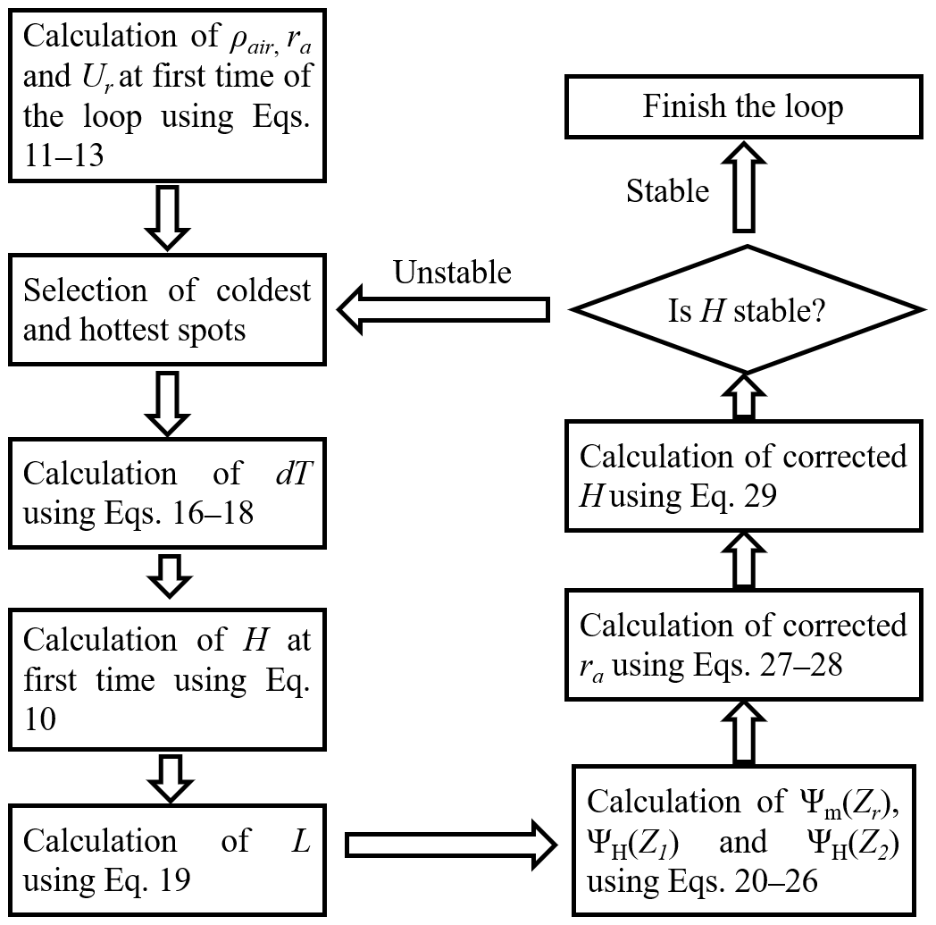
Figure A1 A flowchart of the calculation of sensible heat flux using Monin–Obukhov similarity theory (MOST).

Moreover, it should be noted that H and r_a are interrelated variables in the actual calculation; therefore, the Monin–Obukhov similarity theory (MOST) Monin–Obukhov length (L, unit: m) is introduced for iterative calculation to obtain stable values of H and r_a. The details of MOST are shown in Fig. A1.

The Monin–Obukhov length is a parameter reflecting the turbulent characteristics of the near-surface layer (Eq. A19) (Monin and Obukhov, 1954); Ψ_m(Z_r) is the stability correction function of momentum, and Ψ_H(Z₁) and Ψ_H(Z₂) are the stability correction functions of sensible heat flux (Eqs. A20–A26) (Paulson, 1970).

$$\begin{array}{}\text{(A19)}& L={\displaystyle \frac{{\mathit{\rho }}_{\text{air}}{C}_{\mathrm{p}}{U}_{\mathrm{f}}^{\mathrm{3}}{T}_{\mathrm{s}}}{kgH}}\end{array}$$

Here, g is the acceleration due to gravity (9.81 m s⁻²). While L > 0, indicating a stable state, Ψ_m(Z_r), Ψ_H(Z₁), and Ψ_H(Z₂) are calculated as follows.

$$\begin{array}{}\text{(A20)}& {\displaystyle }{\mathrm{\Psi }}_{\mathrm{m}}\left(Z_{\mathrm{r}}\right)={\displaystyle \frac{-\mathrm{5}{Z}_{\mathrm{r}}}{L}}\text{(A21)}& {\displaystyle }{\mathrm{\Psi }}_H\left(Z_{\mathrm{1}}\right)={\displaystyle \frac{-\mathrm{5}{Z}_{\mathrm{1}}}{L}}\text{(A22)}& {\displaystyle }{\mathrm{\Psi }}_H\left(Z_{\mathrm{2}}\right)={\displaystyle \frac{-\mathrm{5}{Z}_{\mathrm{2}}}{L}}\end{array}$$

While L < 0, indicating an unstable state, Ψ_m(Z_r), Ψ_H(Z₁), and Ψ_H(Z₂) are calculated as follows.

$$\begin{array}{}\text{(A23)}& {\displaystyle }\begin{array}{rl}{\mathrm{\Psi }}_{\mathrm{m}}\left(Z_{\mathrm{r}}\right)=& \mathrm{2}\ln \left({\displaystyle \frac{\mathrm{1}+{\mathit{\zeta }}_{Z_{\mathrm{r}}}}{\mathrm{2}}}\right)+\ln \left({\displaystyle \frac{\mathrm{1}+{\mathit{\zeta }}_{Z_{\mathrm{r}}}^{\mathrm{2}}}{\mathrm{2}}}\right)\\ & +\mathrm{2}\arctan \left({\mathit{\zeta }}_{Z_{\mathrm{r}}}\right)+\mathrm{0.5}\mathit{\pi }\end{array}\text{(A24)}& {\displaystyle }{\mathrm{\Psi }}_H\left(Z_{\mathrm{1}}\right)=\mathrm{2}\ln \left({\displaystyle \frac{\mathrm{1}+{\mathit{\zeta }}_{Z_{\mathrm{1}}}^{\mathrm{2}}}{\mathrm{2}}}\right)\text{(A25)}& {\displaystyle }{\mathrm{\Psi }}_H\left(Z_{\mathrm{2}}\right)=\mathrm{2}\ln \left({\displaystyle \frac{\mathrm{1}+{\mathit{\zeta }}_{Z_{\mathrm{2}}}^{\mathrm{2}}}{\mathrm{2}}}\right)\text{(A26)}& {\displaystyle }{\mathit{\zeta }}_z={\left(\mathrm{1}-{\displaystyle \frac{\mathrm{16}Z}{L}}\right)}^{\mathrm{0.25}}\end{array}$$

While L=0, indicating a neutral state, Ψ_m(Z_r) = Ψ_H(Z₁) = Ψ_H(Z₂) = 0. Then, iterative calculation is carried out to correct H (Eqs. A27–A29).

$$\begin{array}{}\text{(A27)}& {\displaystyle }{U}_{\mathrm{f}}^{\ast }={\displaystyle \frac{k{U}_{\mathrm{r}}}{\ln \left(Z_{\mathrm{r}}/z_{\text{0\hspace{0.17em}m}}\right)-{\mathrm{\Psi }}_{\mathrm{m}}\left(Z_m\right)}}\text{(A28)}& {\displaystyle }{r}_{\mathrm{a}}^{\ast }={\displaystyle \frac{\ln \left(\frac{Z_{\mathrm{2}}}{Z_{\mathrm{1}}}\right)-{\mathrm{\Psi }}_H\left(Z_{\mathrm{1}}\right)-{\mathrm{\Psi }}_H\left(Z_{\mathrm{2}}\right)}{k{U}_{\mathrm{f}}^{\ast }}}\text{(A29)}& {\displaystyle }H={\displaystyle \frac{{\mathit{\rho }}_{\text{air}}{C}_{\mathrm{p}}\text{dT}}{r_{\mathrm{a}}^{\ast }}}\end{array}$$

Several iterations were carried out until the value of H was stable. Then, Eq. (A1) was used to calculate λET. However, it should be noted that the entire estimated energy component was an instantaneous value including latent heat; therefore, the concept of the evaporation fraction (Λ) was used to temporally scale up from the instantaneous value to the daily ET. The evaporation fraction was defined as the ratio of latent heat to available energy (e.g., R_n−G) (Eq. A30). Several studies have indicated that the evaporation fraction can be regarded as constant throughout the day (Crago, 1996); therefore, the daily ET can be calculated as follows.

$$\begin{array}{}\text{(A30)}& {\displaystyle }\mathrm{\Lambda }={\displaystyle \frac{\mathit{\lambda }\text{ET}}{R_{\mathrm{n}}-G}}\text{(A31)}& {\displaystyle }{\mathrm{ET}}_{\mathrm{daily}}={\displaystyle \frac{\mathrm{\Lambda }(R_{\text{daily}}-G_{\text{daily}})}{\mathit{\lambda }}}\end{array}$$

Here, ET_daily, R_daily, and G_daily are the daily evapotranspiration, daily net radiation, and daily soil heat flux, respectively. Finally, the daily ET value was calculated. More details about SEBAL can be found in Bastiaanssen et al. (1998a).

Appendix B: Ratio of interpolated pixels of land surface temperature data

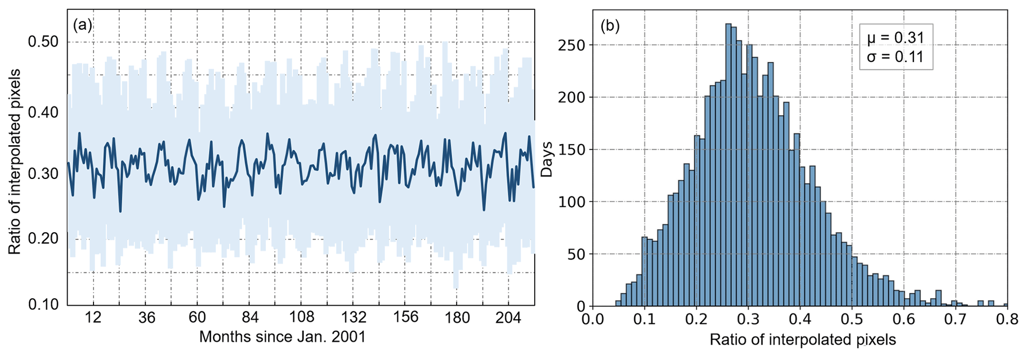
Figure B1 Ratio of interpolated pixels of land surface temperature (MOD11) data: (a) time series of interpolated pixels per month over 2001–2018 and (b) histogram of the ratio of interpolated pixels.