the Creative Commons Attribution 4.0 License.
the Creative Commons Attribution 4.0 License.
 | 06 Aug 2021
CAMELS-AUS: hydrometeorological time series and landscape attributes for 222 catchments in Australia
Keirnan J. A. Fowler
Suwash Chandra Acharya
Nans Addor
Chihchung Chou
Murray C. Peel
This paper presents the Australian edition of the Catchment Attributes and Meteorology for Large-sample Studies (CAMELS) series of datasets. CAMELS-AUS (Australia) comprises data for 222 unregulated catchments, combining hydrometeorological time series (streamflow and 18 climatic variables) with 134 attributes related to geology, soil, topography, land cover, anthropogenic influence and hydroclimatology. The CAMELS-AUS catchments have been monitored for decades (more than 85 % have streamflow records longer than 40 years) and are relatively free of large-scale changes, such as significant changes in land use. Rating curve uncertainty estimates are provided for most (75 %) of the catchments, and multiple atmospheric datasets are included, offering insights into forcing uncertainty. This dataset allows users globally to freely access catchment data drawn from Australia's unique hydroclimatology, particularly notable for its large interannual variability. Combined with arid catchment data from the CAMELS datasets for the USA and Chile, CAMELS-AUS constitutes an unprecedented resource for the study of arid-zone hydrology. CAMELS-AUS is freely downloadable from https://doi.org/10.1594/PANGAEA.921850 (Fowler et al., 2020a).
- Article
(3393 KB) - Full-text XML
- Version 2025
- BibTeX
- EndNote


For some time, the ideals of “comparative hydrology” and “large-sample hydrology” have been advanced as complementary and necessary components of hydrology (e.g. Falkenmark and Chapman, 1989; Andréassian et al., 2006; Gupta et al., 2014). Alongside traditional hydrological studies, which may focus on a single catchment or possibly compare results among several catchments within a region, large-sample studies aim to establish the generality of results and to test paradigms applicable on regional to global scales (e.g. McMahon et al., 1992; Peel et al., 2004; Kuentz et al., 2017; Ghiggi et al., 2019; Mathevet et al., 2020). Large samples of catchments are also insightful for certain tasks, such as prediction in ungauged basins (e.g. Pool et al., 2019; Kratzert et al., 2019b) or training and evaluation of machine learning algorithms (e.g. Kratzert et al., 2018; Shen, 2018; Kratzert et al., 2019a). Thus, large-sample studies are a growing component of recent hydrological research (see review by Addor et al., 2019).
However, issues of data availability and commensurability, which are endemic to environmental sciences, are exacerbated for large-sample hydrology. Large samples may cross jurisdictions or data providers or require harmonisation across different data formats or nomenclatures (e.g. hydrometric-data quality codes and flags) and are more likely to suffer from spatial gaps due to different data sharing policies of water agencies (Viglione et al., 2010; Addor et al., 2019). Thus, the importance of FAIR data (findable, accessible, interoperable and reusable; see Wilkinson et al., 2016 and the Open Data Charter, 2015) in hydrology is amplified in large-sample hydrology, and there is a clear need for open publication of datasets wherever possible to allow equal access. Such policies also encourage hydrologists to work across boundaries – an important ideal since the spatial distribution of hydrologists globally reflects neither the spread of interesting hydrological environs nor the pressing need for hydrological insights to inform policy.
Responding to these needs, multiple recent projects have publicly released large-sample hydrological datasets (e.g. Arsenault et al., 2016; Do et al., 2018; Lin et al., 2019; Linke et al., 2019; Olarinoye et al., 2020). Here we contribute to one such ongoing project – the Catchment Attributes and Meteorology for Large-sample Studies, or CAMELS, project. Originally launched for the United States (Newman et al., 2015; Addor et al., 2017), CAMELS datasets now exist for Chile (Alvarez Garreton et al., 2018), Great Britain (Coxon et al., 2020) and Brazil (Chagas et al., 2020). The defining features of a CAMELS dataset are that they complement data on streamflow (which are often publicly available) with other data types: (i) pre-processed climatic data for each catchment, such as would be required to run a hydrological model, and (ii) catchment attributes which characterise various aspects of the catchment without the need for field visitation (impractical for large samples). They also support download of the entire dataset in contrast to agency websites, which may only support one-at-a-time download (if at all). Lastly, whereas government agencies reserve the right to retrospectively re-process their streamflow data (e.g. due to rating curve changes), CAMELS datasets enable repeatability because a given CAMELS release effectively “freezes” the data, creating a consistent version that is available indefinitely via a persistent digital object identifier (DOI).
The present dataset focusses on the continent of Australia, including the southern state of Tasmania but excluding other Australian territories. Australia is the world's sixth-largest country (approximately 7.7 × 10⁶ km2) and is comparable in size to the conterminous USA or Europe, but the hydrologically active parts of the country tend to be limited to coastal regions, with the interior being semi-arid or arid (Fig. 1; see also Knoben et al., 2018). Thus, dense gauging of streamflow covers only a small proportion of the total area, with the remaining areas providing few gauged locations. While sparsely gauged, the dry parts of Australia provide interesting arid-zone catchment examples, many of which are included in the CAMELS-AUS, the Australian edition, dataset. In addition to arid regions, Australia includes northern areas with tropical climate and southern areas with temperate climate.

Figure 1Location of the 222 CAMELS-AUS flow gauging stations and catchments, along with mean annual precipitation (from Jones et al., 2009) and Australian states and territories.
This paper is structured as follows. In Sect. 2 we describe the rationale for the dataset, including considerations of why Australian hydroclimate is interesting and relevant to hydrologists globally; and factors shaping the dataset, including local data availability. Section 3 provides a technical description of the dataset and forms the bulk of the paper. Sections 4 and 5 explain CAMELS-AUS data availability and conclude the paper, respectively.
This section lays out the motivations underpinning the release of this dataset for Australia. It also outlines why CAMELS-AUS takes its present form, including two chief aspects: catchment selection and inclusion of local versus global datasets.
2.1 Motivation: Australian hydroclimate and its place in the study of arid-zone hydrology and hydrology under climatic change
Every region on earth is unique and has characteristics of interest for hydrological study. Within Australia and for CAMELS-AUS, three characteristics are noted here. Firstly, Australia contains many arid landscapes, and considerable advances in arid-zone hydrology have been made there (e.g. Western et al., 2020). CAMELS-AUS contains more than 20 arid-zone rivers (depending on definition, but see Fig. 1), so the publication of the dataset opens the study of these rivers to a global pool of scientists. Added together with included arid-zone rivers in the USA and Chile (Addor et al., 2017; Alvarez-Garreton et al., 2018), the CAMELS datasets together provide a significant sample for the study of arid-zone hydrology.
Secondly, Australian catchments tend to have lower rainfall-to-runoff ratios, linked to higher evaporative demand. As shown in Fig. 2d, the median rainfall–runoff ratio among Australian catchments is approximately 0.25, compared to approximately 0.4 for the rest of the world. Australian catchments are often water-limited (at least on a seasonal basis), providing different modelling challenges to energy-limited catchments from higher latitudes.
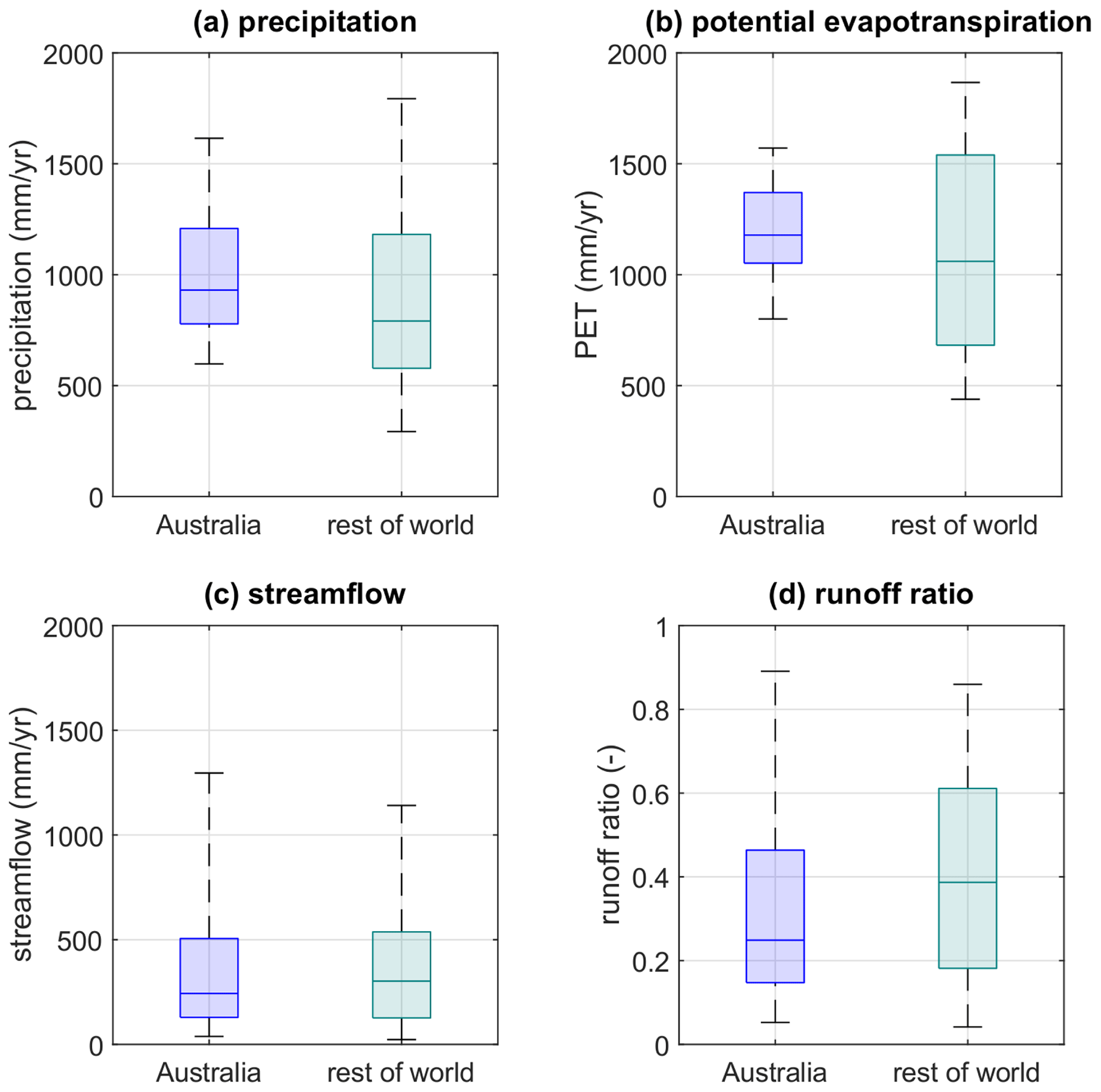
Figure 2Mean annual values of hydrological variables for the global set of 699 catchments presented by Peel et al. (2010; nAustralia=123, nrest of world=576). Boxplots show the 5th, 25th, 50th, 75th and 95th percentiles. Potential evapotranspiration in this dataset is a reference crop estimate using a method similar to Hargreaves' method, as outlined in Adam et al. (2006).
Finally, a notable characteristic of Australian hydroclimatology is its tendency for multi-year spells of climatic anomalies of larger magnitude compared to most other regions of the world (Peel et al., 2005), due partly to the strong influence of climate teleconnections such as the El Niño–Southern Oscillation (ENSO; e.g. Peel et al., 2002; Verdon-Kidd and Kiem, 2009). Recent severe droughts have affected south-eastern Australia, including the 13-year Millennium Drought (Van Dijk et al., 2014), which provided the opportunity for knowledge sharing with other drought-prone regions (Aghakouchak et al., 2014) and supplied many case studies of hydrological model failure (i.e. the high bias and low model performance in differential split sample testing reported by e.g. Saft et al., 2016), which are under ongoing investigation (e.g. Fowler et al., 2020b). In the context of providing credible runoff projections, case studies of long droughts are the only means by which hydrologists can test hypotheses regarding how catchments respond physically to the onset of drier conditions, including aspects of long “memory” (e.g. Fowler et al., 2020b) and potential to shift behaviour, possibly in a quasi-permanent fashion (e.g. Peterson et al., 2021). Thus, it is hoped that the public release of datasets such as CAMELS-AUS may hasten scientific progress towards more defensible and robust hydrological models.
2.2 Context: hydrometeorological monitoring in Australia
Systematic climatic measurement in Australia extends back to the late 1800s (e.g. Ashcroft et al., 2014), with widespread streamflow gauging of headwater catchments commencing from the 1950s and '60s. Meteorological monitoring is the responsibility of a federal Bureau of Meteorology (BOM), but streamflow monitoring falls to the states and territories of Australia rather than the federal government (Skinner and Langford, 2013). Thus, Australian streamflow data have historically been dispersed between its six states and two territories (Fig. 1), and while quality control is relatively well established, methods and formats (e.g. quality codes and flags) are not consistent between states and territories. Since the 2000s this situation has partially been rectified after federal legislation required the BOM to collate data from the states under new “water information” powers (Vertessy, 2013).
2.3 Catchment choice: the Hydrologic Reference Stations dataset
Under its new responsibilities the BOM initiated several national hydrological projects, one of which is called the Hydrologic Reference Stations project (Turner et al., 2012). This project selected a large set of gauging stations, each on unregulated streams, to serve as a “platform to investigate long-term trends in water resource availability” (Turner et al., 2012, p. 1555). The project has a website for provision of streamflow data to the public (http://www.bom.gov.au/water/hrs/, last access: 29 July 2021).
We adopted the Hydrologic Reference Stations as the basis for CAMELS-AUS for three reasons:
-
The selection criteria used by the BOM, including record length, lack of regulation and stationarity of anthropogenic influence (see Sect. 3.2), are consistent with the aim of the CAMELS project to provide high-quality scientific data.
-
Considerable effort has already been expended by the BOM to standardise and quality-check the streamflow data, which was only possible via contacts with state agencies that are not necessarily available to academic authors (for an example, see BOM, 2020). It is logical to take advantage of this prior effort.
-
The Hydrologic Reference Stations have attained a degree of acceptance within the Australian hydrological community, partly due to extensive consultation with stakeholders during development (see Sect. 3.2). Also, they have been adopted by numerous academic studies (e.g. Zhang et al., 2014, 2016; Wright et al., 2018; McInerney et al., 2017; Fowler et al., 2016, 2018, 2020b).
It is noted that this choice is not intended to limit future inclusion of a wider range of stations and catchments. We envisage that the Hydrologic Reference Stations may provide the nucleus for future versions of the CAMELS-AUS dataset, while the current selection provides a sensible and pragmatic starting point. The Hydrologic Reference Station dataset itself may be subject to future expansion, which would inform future CAMELS-AUS versions. Furthermore, whereas the Hydrologic Reference Stations project, by definition, sought catchments which are minimally disturbed (or at least having stationarity of anthropogenic influence), future versions could be more inclusive so as to cater for studies examining diverse anthropogenic influences including changes over time – an approach already taken by CAMELS-GB (Great Britain; Coxon et al., 2020) and CAMELS-BR (Brazil; Chagas et al., 2020). In summary, the current form of CAMELS-AUS should not be interpreted as setting a norm for future versions (or other datasets).
2.4 Local versus global datasets
A key choice in developing CAMELS-AUS was whether to use local or global datasets (or both) when extracting hydrometeorology time series and catchment attributes. On the one hand, global datasets are important to facilitate intercontinental comparisons. On the other hand, when local datasets are available, they are generally the highest-quality information that exists for a given region (e.g. Acharya et al., 2019). With the advent of large-sample hydrology, it is now possible to conduct near-global studies using very large samples of catchments (e.g. over 2000 in Mathevet et al., 2020), and future studies might compose such large samples by combining continental-scale datasets like the various CAMELS. However, the lack of standardised approaches and sources between national large-sample datasets remains a key limitation of large-sample studies (Addor et al., 2019).
The approach followed by the CAMELS datasets so far is to use the best possible data available for each country, so national datasets have been prioritised over global datasets. In some cases, global datasets have been employed, for instance the Global Lithological Map (Hartmann and Moosdorf, 2012) in CAMELS datasets for the USA and Chile or the Multi-Source Weighted-Ensemble Precipitation (Beck et al., 2017) in CAMELS-CL. But overall, the best national data products were selected for each country, leveraging the knowledge of CAMELS creators. This enables global users, who may not be familiar with these national products, to benefit from this local knowledge. It also gives direct access to the best available data to users whose study focusses on catchments from a single country (see e.g. intercomparisons in Acharya et al., 2019). In keeping with this approach, the priority was given to national data products to produce CAMELS-AUS.
In parallel, efforts are ongoing to increase the consistency among the CAMELS datasets (in terms of data products used to derive the time series and catchment attributes and also naming conventions and data format; see Addor et al., 2019) in order to create a dataset that is globally consistent. This is part of a second phase, which will build upon the current phase, which is focussed on the release of national products, such as CAMELS-AUS. To contribute to this effort, we have supplied the CAMELS-AUS catchment boundaries and gauge locations. Because of these ongoing efforts, our expectation is that the data introduced here, derived from Australian sources, will in time be complemented by data derived from global datasets.
The previous section outlined key decisions made for CAMELS-AUS; i.e. it is based on the Hydrologic Reference Stations, and its data are derived from Australian rather than global sources. This section provides more detail and presents each aspect of the dataset in turn. Work not undertaken by the present authors (e.g. earlier efforts by the BOM for the Hydrologic Reference Stations project) is clearly marked. In many cases, sub-sections end with an “Included in dataset” section to clearly outline items in the online repository related to the sub-section text.
Before presenting the details, we note that the online repository of the dataset (Fowler et al., 2020a) includes the following:
-
a file containing the overall attribute table containing all non-time-series data (see Tables 1, 3 and 4);
-
27 time series files, each containing data for all catchments for a given hydroclimatic variable (see Table 2); and
-
extra files such as shapefiles and readme files as noted below.
Table 1Basic catchment information provided in the attribute table of CAMELS-AUS.
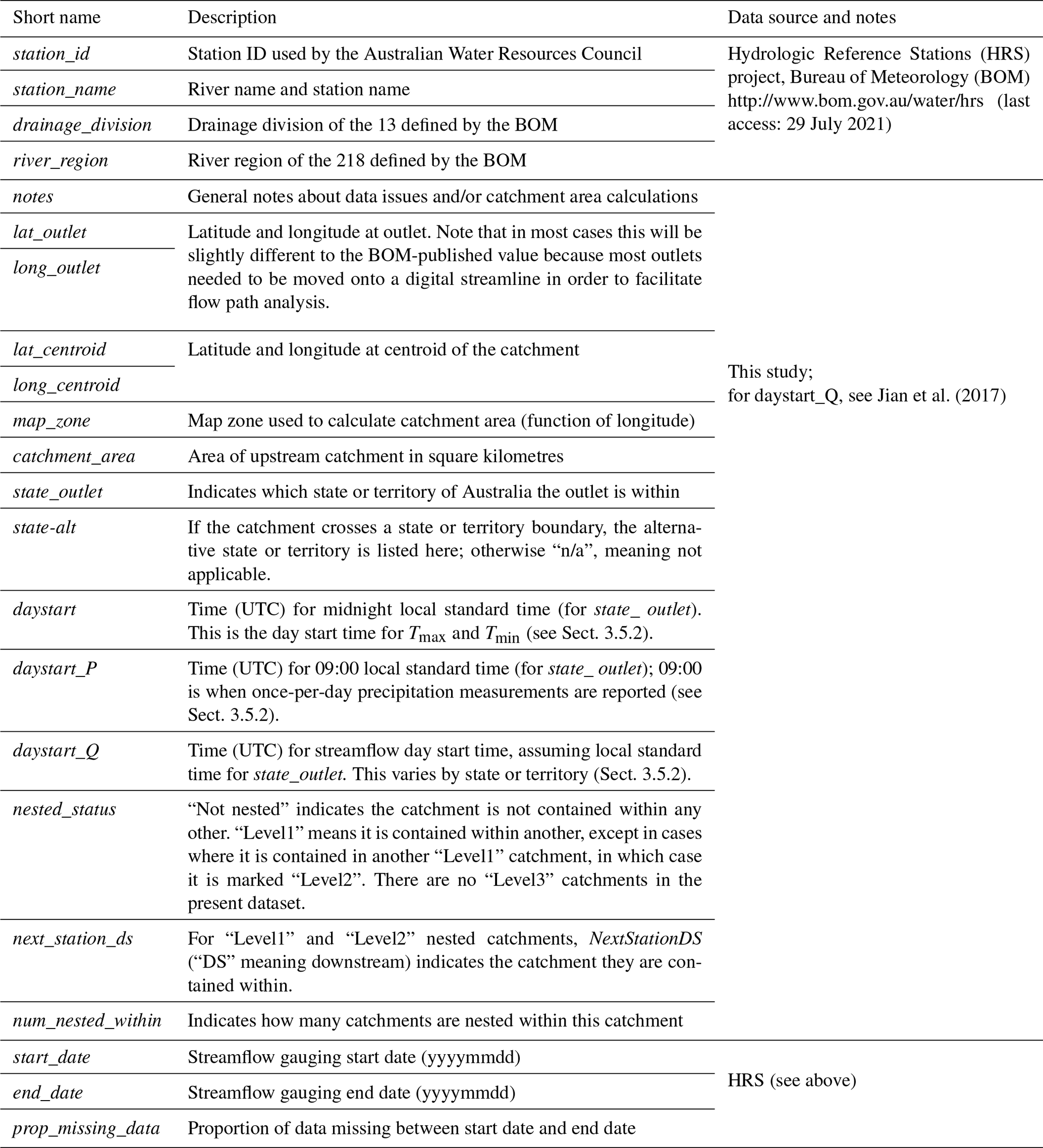
Table 2Hydrometeorological time series data supplied with CAMELS-AUS. All time steps are daily. All non-streamflow data were processed as part of the CAMELS-AUS project to extract catchment averages from Australia-wide Australian Water Availability Project (AWAP) and Scientific Information for Land Owners (SILO) grids.
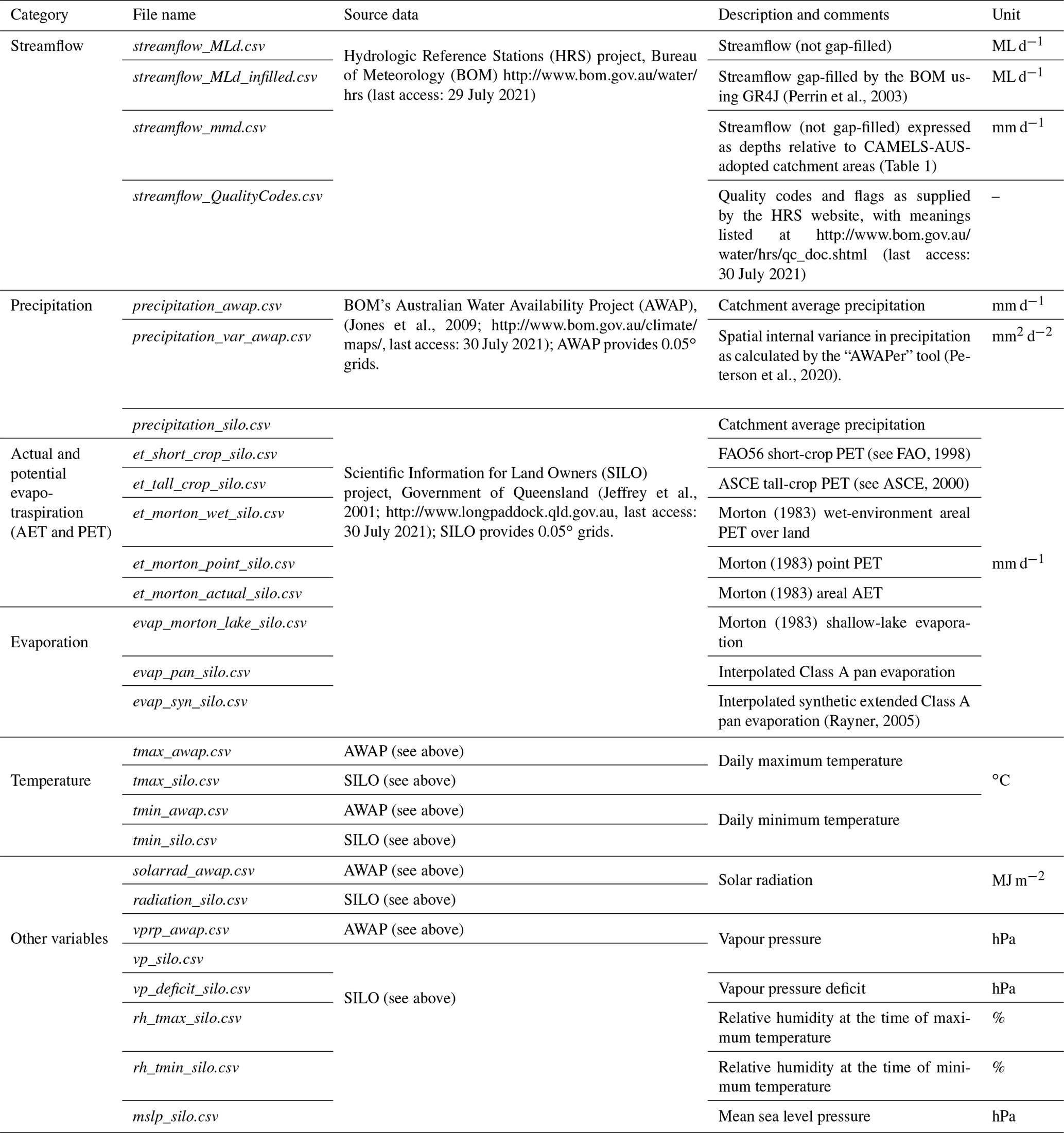
Table 3Flow uncertainty information, climatic indices and streamflow signatures provided in the attribute table of CAMELS-AUS.
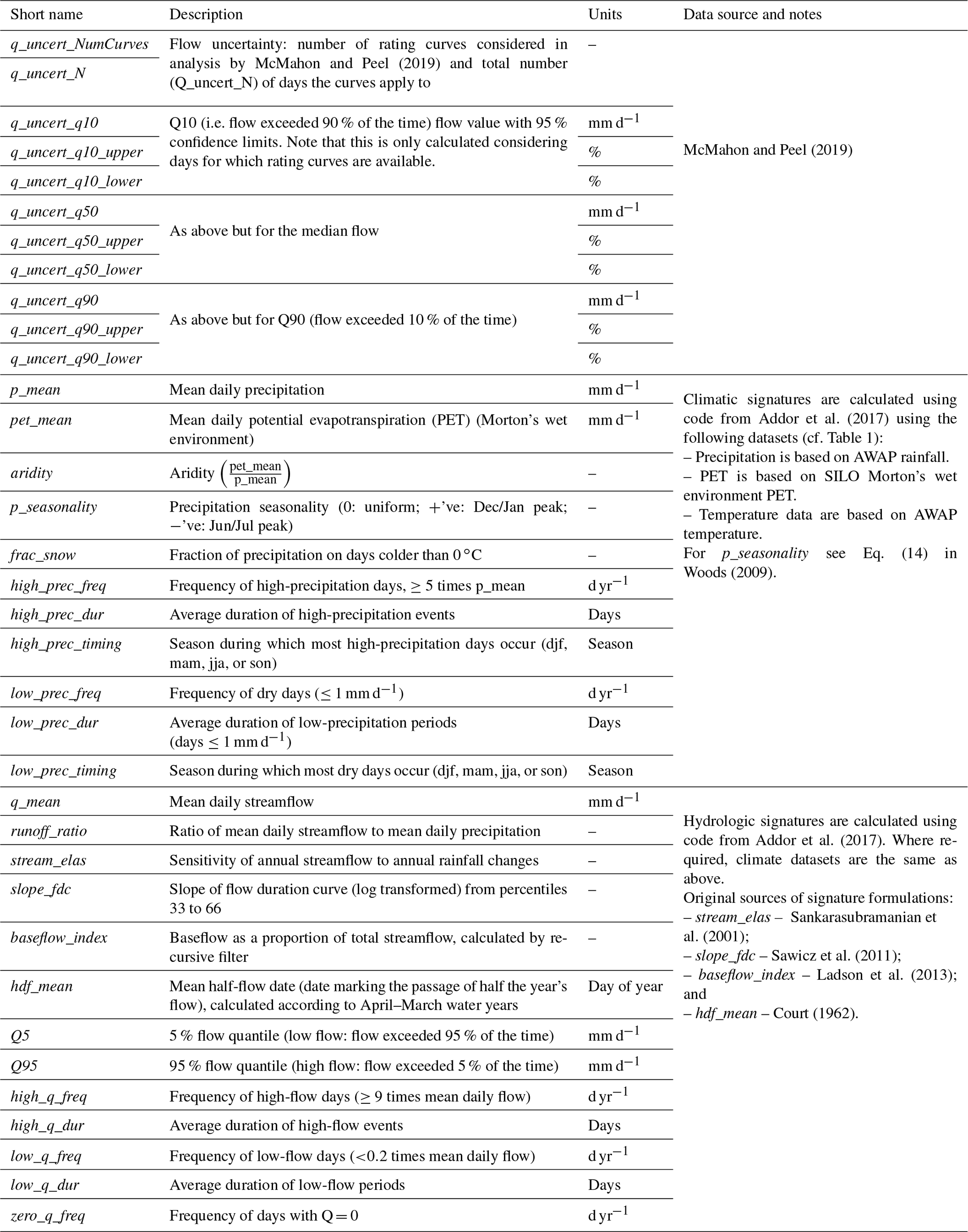
Table 4Catchment attributes included in the attributes table of CAMELS-AUS (apart from climatic and hydrologic indices).

3.1 Catchment selection rules
Given the decision (Sect. 2.2 above) to base the CAMELS-AUS dataset on the BOM's Hydrologic Reference Stations, this sub-section summarises the process of catchment selection undertaken earlier by the BOM, as described in Turner et al. (2012).
-
Initial selection: 246 potential stations were initially selected based on the three criteria of (i) record length (minimum of 1975 onwards), (ii) availability of data including historic rating curve information and (iii) lack of regulation by large dams.
-
Invitation for stakeholders to suggest additional stations: BOM consulted with 70 stakeholders from federal, state and territory agencies and water authorities, who were given the opportunity to add new stations to the list. This enlarged the list to 362 stations.
-
Targeted fact-finding: to elicit information about each candidate station and catchment, the relevant agencies were asked a series of questions about the catchments in their jurisdiction relating to both past and present practices. Topics included diversions, irrigation structures, upstream point source discharge, land clearing, forestry, urbanisation, fire and farm dams.
-
Final selection: the final selection process considered all the above information. A good coverage of Australia's various hydroclimatic regions was desired, although this is inherently limited by the coverage of the gauging network. Where possible, only stations with < 5 % missing data and <10 % change in forest cover were selected.
The above process provided the first version of the Hydrologic Reference Stations, with a total of 221 catchments. A subsequent update in 2015, which included a detailed review and update of streamflow data up to 2014 (BOM, 2020), resolved to retain all existing stations and add one more (ID 215207). Thus, the final number of stations is 222 (Fig. 1).
Included in dataset. The following variables are provided in the CAMELS-AUS attribute table (see Table 1): station ID, station name (including river name and station name), drainage division and river region (out of 13 drainage divisions and 218 river regions across Australia). Unfortunately, information is not available about which catchments were included or excluded under the above rules.
3.2 Catchment boundaries
For all but 10 of the catchments, catchment boundaries were derived via flow path analysis (using Esri's Arc Hydro) of topographic data undertaken by the authors. The input data were (i) the post-processed and hydrologically enforced DEM of Gallant et al. (2012), which is derived from the 1 s (approximately 30 m) grid Shuttle Radar Topography Mission (SRTM) dataset, and (ii) the location of the streamflow gauges as provided by the BOM. The Arc Hydro analysis determines the apparent position of streams from the DEM data, and it was found that the published locations rarely fall precisely on these digital streamlines. The mismatch is unsurprising given that location data may be decades old, and significant figures may have been truncated with the passage of data between databases (or never reported in the first place). Also, the position of the digital streamline may or may not match reality, particularly in flat landscapes. To derive catchment areas, the BOM-published gauge locations were shifted to the nearest streamline with expected catchment area. This movement was generally less than 200 m.
As noted, this method was used for most catchments, with the following exceptions:
-
For the six largest catchments (A0030501, A0020101, G8140040, G9030250, 424002 and 424201A), this process was not undertaken due to excessive computational requirements. For context, the largest catchment is approximately the size of the United Kingdom (see Fig. 1).
-
For a further four catchments (A2390519, A2390523, 307473 and 606185), the Arc Hydro process resulted in a catchment boundary that was inconsistent with the boundaries displayed on the Hydrologic Reference Station website. Although degraded for fast mapping, the website boundaries show the approximate position of the boundary as agreed with stakeholders and agencies who have local knowledge. Therefore, in cases of obvious mismatch, the Arc Hydro-derived boundaries were assumed to be in error. Despite the “blockiness” of the website boundaries, they were considered to be a better option for these four catchments.
For these 10 catchments a protocol was developed to read the website's .json file to extract the boundary vertices. The website boundaries were then adopted. Note that more detail on the above considerations, including a selection of figures, is given in the dataset within the readme file README_CAMELS_AUS_Boundaries.pdf.
Included in dataset. The main inclusions are a point shapefile of adopted gauge locations and a polygon shapefile of adopted catchment areas. Further information included are a point shapefile of BOM-published gauge locations, polygon shapefile of website-mapped boundaries, and readme file explaining the above logic but in more detail and with figures. As listed in Table 1, the CAMELS-AUS attribute table lists the coordinates of the catchment outlet and centroid, along with notes which expand on issues listed above, on a catchment-by-catchment basis.
3.3 Catchment area and nestedness
To calculate catchment areas, the catchment boundaries were first projected into the appropriate local coordinate system under the Map Grid of Australia (MGA). Due to Australia's size, the MGA defines different coordinate systems based on longitude. Using the catchment centroid, each catchment was placed within a zone, and this zone was used to calculate area using the standard tool within Esri's ArcMap. Inspection of catchment boundaries revealed that some of the catchments are “nested” (i.e. entirely contained) within others, for example, when two gauges lie on the same stream (one downstream of the other) and both have been included in the dataset. The upstream (i.e. entirely contained) catchments are clearly marked in the CAMELS-AUS attribute table (see Table 1). Catchments containing nested catchments are also marked.
Before moving on from considerations of spatial data, it is noted that (i) CAMELS-AUS does not come with a spatial layer for the river network, (ii) users may find the 15 s Hydrosheds River Network (http://www.hydrosheds.org/downloads, last access: 30 July 2021) or the BOM Geofabric v2 SH network (http://www.bom.gov.au/water/geofabric/download.shtml, last access: 30 July 2021) useful, and (iii) the reason these are not included in CAMELS-AUS is because of licensing concerns (for Hydrosheds) and file size concerns (for the Geofabric).
Included in dataset. The following variables are provided in the CAMELS-AUS attribute table (see Table 1): catchment area, map zone and three indicators related to nestedness (NestedStatus, NextStationDS, NumNestedWithin).
3.4 Streamflow data and uncertainty
Streamflow time series data are provided by the BOM in two variants: non-gap-filled, and gap-filled. The gap-filled variant is filled using the daily rainfall–runoff model GR4J (Perrin et al., 2003), but the BOM has not published further methodological details about calibration method, validation procedures or the specifics of the interpolation method. In addition to the streamflow data, the BOM also provides quality codes and flags. As mentioned in Sect. 2.1, the quality codes and flags of each state of Australia are different, but the BOM has harmonised these to a common set (http://www.bom.gov.au/water/hrs/qc_doc.shtml, last access: 30 July 2021). For CAMELS-AUS, these data are supplied as follows. Firstly, summary statistics about period of record (start date, end date and proportion of missing data) are provided in the attribute table, as listed in Table 1. Regarding time series data (Table 2), each of the above three data types (gap-filled, non-gap-filled, and quality codes and flags) are provided within CAMELS-AUS exactly as supplied by the BOM, except that they are presented as a single file across all catchments. In addition, since the units of the streamflow files are ML d−1, whereas modelling studies typically use mm d−1, CAMELS-AUS provides an additional streamflow time series file in mm d−1.
Figure 3 shows that CAMELS-AUS stations are typically long-term gauges, with the shortest record being 29 years. All but 17 gauges commence by 1975 (in line with the selection rules in Sect. 3.1), and all but 22 of the records contain data up until the cut-off date for this dataset, which is 31 December 2014. Thus, records longer than 40 years are typical (Fig. 3b). Figure 3a considers both the record extent and missing data to determine the overall data availability for different overlapping periods. The data availability for the periods starting in 1965 and 1970 are lower than the others, as expected given the remarks about record length. An increase in missing data post-1990 means that the data availability curves decrease slightly for the most recent period (dark blue).
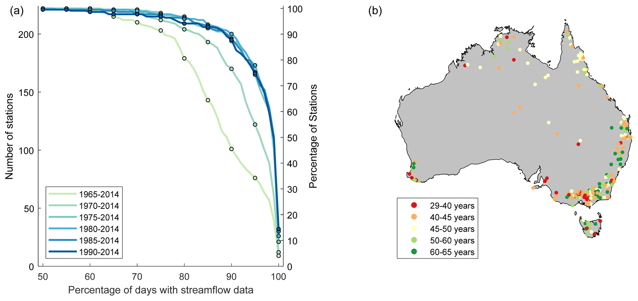
Figure 3Plot after Coxon et al. (2020) showing (a) number of stations with percentage of available streamflow data for different periods and (b) length of the flow time series for each gauge.
Information about streamflow uncertainty is provided with CAMELS-AUS (Table 1) from an earlier study by McMahon and Peel (2019). McMahon and Peel (2019) examined available rating curve data for 166 of the 222 stations, developed rating curves based on Chebyshev polynomials, and estimated uncertainties using an approach which considered regression error and uncertainty in water level. The original authors post-processed their data to provide the following statistics (Table 3) for CAMELS-AUS: (i) number of separate rating curves considered for a given station (median value across all stations was 3); (ii) number of days considered across all curves (median value was ∼14 700 or ∼40 years); (iii) low, medium and high flow rates in mm d−1 (flow rates exceeded 90 %, 50 % and 10 % of the time over days considered by the curves); and (iv) 95 % confidence intervals around low, medium and high flow rates, expressed in percentage terms. However, for some stations considered by McMahon and Peel (2019) the above data are not supplied in full for the following reasons: (a) the percentile flow is zero (cease to flow), leading to undefined relative uncertainty estimates due to the need to divide by zero, or (b) the percentile flow is outside the rated range, in which case neither upper nor lower bounds are reported for that flow. In a small number of cases the uncertainty bound numbers are very high, and these cases are generally associated with near-cease-to-flow conditions. For example, the highest value of Q_uncert_Q10_upper (refer to Table 3 for naming conventions) occurs for catchment 919309A, for which Q10 is 0.000023 mm d−1, but the upper bound is 0.05 mm d−1, which is >2000 times higher. Thus, Q_uncert_Q10_upper for this catchment is 201 400 %.
Included in dataset. The dataset includes three streamflow time series files, as explained above and listed in Table 2; one time series file for streamflow quality codes and flags; and the following attributes in the CAMELS-AUS attribute table: three attributes related to record extent and availability (start date, end date, prop_missing_data; see Table 1) plus 11 attributes related to streamflow uncertainty (Q_uncert_NumCurves, Q_uncert_N, Q_uncert_Q10, Q_uncert_Q10_upper, Q_uncert_Q10_lower, Q_uncert_Q50, Q_uncert_Q50_upper, Q_uncert_ Q50_lower, Q_uncert_Q90, Q_uncert_Q90_upper, Q_uncert_Q90_lower; see Table 3).
3.5 Hydrometeorological time series
3.5.1 Availability of gridded hydrometeorological data in Australia
It is common practice in large-sample hydrology studies to derive climate time series inputs by processing gridded data rather than directly using gauged point information (as is still common in industry). The first Australia-wide gridded climate product was the Scientific Information For Land Owners (SILO) project of the government of the State of Queensland (Jeffrey et al., 2001). Later, the BOM developed a separate set of climate grids under the Australian Water Availability Project (AWAP; Jones et al., 2009). SILO and AWAP are similar: they are both interpolated products based purely on the BOM's climate monitoring sites and (where relevant) incorporating topography as a co-variate. They both output grids at a resolution of 0.05∘ × 0.05∘ (approximately 5 km). However, the datasets differ in the variables they provide: AWAP provides precipitation, temperature, vapour pressure and radiation, all of which SILO also provides in addition to vapour pressure deficit and, importantly for modelling studies, various formulations of potential evapotranspiration (PET). They also differ in spatial interpolation method: the SILO method forces an exact match to measured values, whereas AWAP does not (Tozer et al., 2012). Both AWAP and SILO are commonly used in Australia. Rather than select one dataset over another, CAMELS-AUS includes both datasets and leaves the choice to users. When possible, users are encouraged to compare the datasets to obtain insights into interpolation uncertainty for the forcing data. For all AWAP and SILO variables, time series for each catchment were compiled by the CAMELS-AUS project by calculating the catchment spatial average separately for each day. The full available period was extracted, which for most variables is 1900–2018 (SILO) and 1911–2017 (AWAP). Exceptions to these record extents are noted in the text below.
3.5.2 Limitations arising from conventions for definition of daily time steps
Variables such as precipitation and streamflow are continuous, and formatting into a daily time step requires arbitrary conventions to split continuous time into 24 h periods. For example, the BOM convention is that precipitation is split at 09:00 (all times given in local time) each day, and a daily value refers to the precipitation that occurred over the preceding 24 h. Thus, if the BOM reports 18 mm precipitation for 14 March, this means that 18 mm was recorded between 09:00 13 March and 09:00 14 March. For streamflow, the conventions may vary depending on state or territory, but in collating the HRS data the BOM claims that conventions have been standardised to 09:00 to 09:00 (i.e. the same as precipitation). However, an audit of HRS data conducted by Jian et al. (2017) investigated this standardisation. They report that data from the states of Victoria, New South Wales, Queensland and the Australian Capital Territory (which together account for 168 of 222 stations) were consistent with the 09:00-to-09:00 claim. In contrast, they report that Western Australia (16 stations) data appear to be subject to a 01:00 split (i.e. 8 h earlier than expected), and South Australia and Northern Territory data (25 stations) appear to be subject to a 23:30 split (i.e. 9.5 h earlier than expected). Modellers should be mindful of these points when designing studies and interpreting results since modelling results may be sensitive (Reynolds et al., 2018; Jian et al., 2017) to the day definitions for both precipitation and discharge (and, if relevant, the degree to which they are offset from one another). Regarding PET, the key variables (e.g. temperature) are aligned directly with the day they are reported. This creates a time offset between PET and precipitation. In the experience of the CAMELS-AUS authors, this offset will typically make little difference to the results of, for example, a rainfall–runoff modelling study since PET typically influences streamflow via seasonal, not daily, dynamics in most CAMELS-AUS catchments. In the interest of providing CAMELS-AUS data subject to minimal manipulation, we do not apply a time shift to PET (or any other data), but users may wish to manually shift PET earlier by 1 d to minimise the time offset between precipitation and streamflow.
A further consideration is that, due to Australia's large size, the CAMELS-AUS catchments occupy three different time zones. The majority are in a single zone (UTC + 10:00) covering Queensland, New South Wales, the Australian Capital Territory, Victoria and Tasmania. However, South Australia and the Northern Territory are in a separate zone (UTC + 09:30), while Western Australia uses UTC + 08:00. In addition, daylight savings time is used in South Australia, New South Wales, the Australian Capital Territory, Victoria and Tasmania. During the daylight savings period (typically October to April) 1 h needs to be added to the UTC times stated above. Given this multiplicity of combinations, measurements taken on either side of a state border that are marked with the same timestamp (e.g. 09:00) may, in reality, have been taken at different times.
Unfortunately, these limitations (related to time zones and day definitions) are inherent to the observations, and this then carries across into derivative products such as gridded climate data. In principle, if data were measured continuously it would be possible to redefine the day definitions and thus harmonise across time zones and data products, but unfortunately most observations are only taken once per day rather than continuously. Thus, there is little choice but to accept the use of these data despite these limitations.
3.5.3 Precipitation
AWAP and SILO precipitation are provided in the files precipitation_awap.csv and precipitation_ silo.csv, respectively (Table 2). Users interested in a comparison of AWAP and SILO precipitation are referred to Tozer et al. (2012), who note that the two products vary due to differences in interpolation methods, as noted above. They also assess the impact of adopting these gridded products on rainfall–runoff modelling outcomes, which may be of interest to CAMELS-AUS users.
One further rainfall-related time series file is precipitation_var_awap.csv, which provides, for each day, the spatial variance due to differences between grid cell values within a given catchment. This analysis was conducted using the tool AWAPer (Peterson et al., 2020), and the outputs can be used to understand how representative areal averages are across a given catchment and how this varies with time.
3.5.4 Evaporative demand
As noted, evaporation and evapotranspiration variables are provided by SILO only (Table 2). SILO provides PET estimates for the FAO56 short-crop (Food and Agriculture Organization of the United Nations, 1998) and ASCE tall-crop (ASCE, 2000) methodologies, in addition to three evapotranspiration formulations from Morton (1983), namely point potential, areal wet environment potential and areal actual. Three additional evaporation products are also provided, namely Morton (1983) shallow-lake evaporation, interpolated Class A pan evaporation (which only covers the measured period, 1970 onwards) and synthetic Class A pan evaporation extended to the full SILO period using the method of Rayner (2005). See Table 2 for adopted file names.
3.5.5 Other time series
AWAP time series are provided for a further four variables: daily maximum temperature, daily minimum temperature, vapour pressure (1950 onwards) and solar radiation (1990 onwards). Solar radiation AWAP data have numerous gaps, which have been filled by the average Julian day value: for example, if 5 March is missing, we adopt the average value over all non-missing instances of 5 March. SILO time series are provided for the following variables: daily maximum temperature, daily minimum temperature, vapour pressure, vapour pressure deficit, solar radiation, mean sea level pressure (1957 onwards), relative humidity at time of maximum temperature and relative humidity at time of minimum temperature. See Table 2 for adopted file names.
3.6 Catchment attributes
The following sub-sections, along with Tables 3 and 4, summarise the set of CAMELS-AUS catchment attributes. Spatial distributions of selected attributes are mapped in Fig. 4.
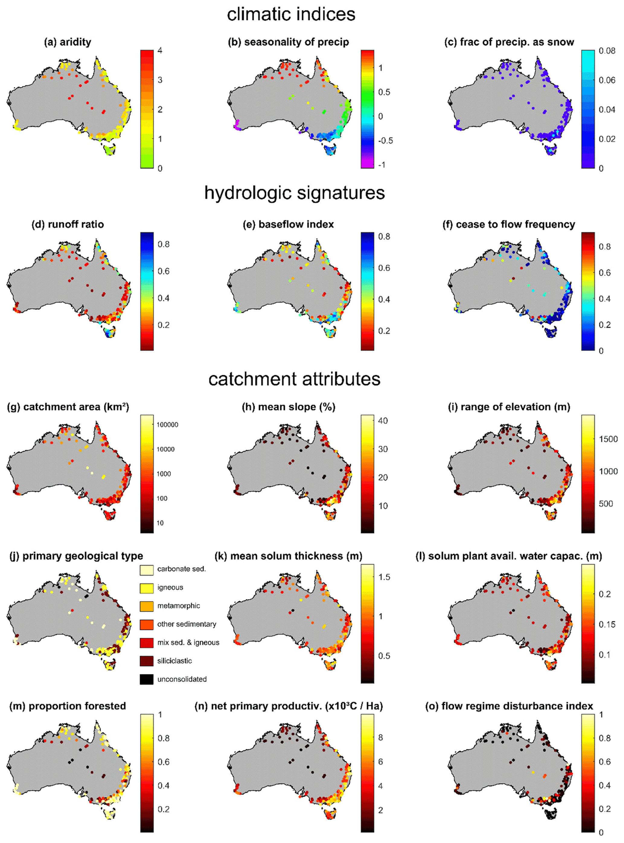
Figure 4Maps of selected climatic indices (a–c), hydrologic signatures (d–f) and other catchment attributes (g–o). For definitions, see Tables 3 and 4.
We note that the CAMELS-AUS dataset owes much to the earlier work of Stein et al. (2011), whose National Environmental Stream Attributes project calculated a broad variety of catchment attributes spatially across Australia, 74 of which are included in the CAMELS-AUS dataset. Stein et al. (2011) calculated these for the upstream area of each stream segment in Australia based on a 250k scale stream and catchment dataset (the BOM Geospatial Fabric v2.1; http://www.bom.gov.au/water/geofabric/, last access: 30 July 2021), and the contribution of the CAMELS-AUS project for the 74 indices is limited to (i) spatially matching each outlet to the appropriate segment (of which there are 1.4 million to choose from) and (ii) sorting through the attributes to identify those relevant to CAMELS-AUS (e.g. not all Stein et al., 2011, attributes relate to the upstream catchment area; others relate to the local area immediately around the stream segment and are thus irrelevant as CAMELS-AUS attributes in nearly all cases).
3.6.1 Climatic indices and streamflow signatures
A total of 11 climatic indices are provided, as listed in Table 3, calculated using the same code used in the original CAMELS (Addor et al., 2017). The code requires input time series of precipitation, temperature and PET, and for this purpose AWAP was used where available (precipitation, temperature), and for PET, SILO Morton Areal Wet Environment PET was used (this combination of inputs is consistent with past modelling studies such as Fowler, 2016, 2018, 2020b). Likewise, 13 streamflow signature indices are provided, as listed in Table 3, also calculated using code from Addor et al. (2017). Together, the climatic and streamflow indices cover a wide range of statistics commonly used to characterise hydroclimate in modelling and regionalisation studies, and their common formulation with Addor et al. (2017) aids intercontinental comparison.
3.6.2 Geology and soils
Geology data are taken from Stein et al. (2011), who in turn derived these data from the 1:1 000 000 scale Surface Geology of Australia. In Table 4 this dataset is cited for brevity as Geoscience Australia (2008), but here we acknowledge the detailed state-by-state work of Liu et al. (2006), Raymond et al. (2007a, b, c), Stewart et al. (2008) and Whitaker et al. (2007, 2008). For each catchment the proportion taken up by each of the seven geological types is provided as separate attributes. Additionally, we follow Alvarez-Garreton et al. (2018) in defining separate categorical attributes for the primary and secondary geological units (see Fig. 4j for a map of the primary types) with their respective areas defined as separate numerical attributes.
Soil data are taken from a variety of sources. The soil depth attribute (SolumThickness) is based on the Atlas of Australian Soils (Isbell, 2002), which divides Australia into soil “map units”, each with associated “principle profile forms” (ppfs) in order of dominance. In turn, the dataset provides estimates (McKenzie et al., 2000) of the distribution of solum thicknesses (as 5th, 50th and 95th percentiles) associated with each ppf. The CAMELS-AUS SolumThickness is defined as a spatial average across the map units that occur in the catchment, where the depth assumed for a given map unit is the median value for its dominant ppf. Soil saturated hydraulic conductivity (ksat) and water holding capacity (solpawhc) are taken from Stein et al. (2011), who in turn derived these data from Soil Hydrologic Properties of Australia (Western and McKenzie, 2004).
3.6.3 Topography and geometry
Maximum elevation and average elevation are each taken from Stein et al. (2011), but because the gauging stations themselves are not features in the Stein et al. dataset, we calculate the elevation at the outlet separately. Catchment slope is calculated as the spatial average of the slope product of Gallant et al. (2012), which is itself based on the 1 s SRTM DEM.
Stein et al. (2011) provide a variety of attributes related to the geometry of the catchment and/or stream network. Each of these are based on the geometry of the streams and catchments defined in the BOM's Geospatial Fabric v2.1 (http://www.bom.gov.au/water/geofabric/download.shtml, last access: 30 July 2021), which itself is based on the 9 s (approximately 270 m) DEM of Hutchinson et al. (2008). The attributes are (i) maximum flow path length upsdist upstream from the outlet; (ii) stream density; (iii) Strahler (1957) stream order at outlet; (iv) elongation ratio; (v) relief, here defined as ratio of the mean and maximum elevations above the outlet; and (vi) relief ratio, here defined as elevation range divided by flow path distance.
Further attributes are defined based on the multi-resolution valley bottom flatness (MRVBF) index of Gallant et al. (2012).
As the name indicates, the index relates to the shape of the landscape and the degree of deposited sediment. As explained in Table 4, the index values contrast erosional (MRVBF = 0) locations with depositional (MRVBF > 0) locations ranging from “small hillside deposits” (MRVBF = 1) through to “extensive depositional basins” (MRVBF = 9). A total of 10 separate attributes are defined based on each integer value (0,1…9) that MRVBF can take, indicating the proportion of the catchment in the given class. Lastly, using an earlier MRVBF version, Stein et al. (2011) analysed how common it is for a stream to pass through erosional landscapes (MRVBF = 0) and defined this as an additional attribute, “confinement”.
3.6.4 Land cover and vegetation
Land cover and vegetation attributes are primarily based on the Dynamic Land Cover Dataset (DLCD), v2 of Lymburner et al. (2015). Across Australia, the DLCD maps 22 land cover classes using MODIS satellite data over rolling 2-year windows, providing 13 separate time slices (January 2002–December 2003, January 2003–December 2004 … January 2014–December 2015). The CAMELS-AUS dataset incorporates these data in three ways:
-
A separate attribute is defined for each land cover class, where the attribute value indicates the temporal average proportion of the catchment taken up by the class over the 13 time slices.
-
Since “proportion forested” is an oft-used catchment attribute, a separate attribute is defined as the sum of the four DLCD classes which mention trees (“trees – closed”, “trees – open”, “trees – scattered” and “trees – sparse”).
-
The time series data themselves are provided in full for each catchment, in a separate spreadsheet Landcover_timeseries.xlsx.
The DLCD dataset is complemented by data from Stein et al. (2011), in turn sourced from the National Vegetation Information System (NVIS; Department of Environment and Water Resources, 2008). Stein et al. (2011) report the proportion of the catchment occupied by NVIS “major vegetation sub-groups” (categories are grasses, forests, shrubs, woodlands and bare). This has considerable overlap with the DLCD, and the reason it is included is because the NVIS also estimates the proportion of these vegetation types that existed in the catchment's “natural” state (pre-1750; note this is pre-European but not pre-Indigenous settlement). For each of the five categories, the NVIS provides natural pre-1750 (“_n') and “extant' (meaning current, “_e') statistics.
3.6.5 Anthropogenic influences
Anthropogenic influences are relevant to CAMELS-AUS because some catchments are minimally disturbed (e.g. pre-European vegetation cover, few roads), while others, although unregulated, are nonetheless significantly changed from their natural state (e.g. due to agricultural land use, small private (farm) dams, small towns and/or paved roads). Data on anthropogenic influences are taken from Stein et al. (2011) and based on earlier work with the same lead author (Stein et al., 2002). The earlier study aimed to identify the “wild” rivers of Australia by quantifying human impacts on two broad categories: the flow regime (sub-categories: impoundments, flow diversions and levee banks) and the catchment (sub-categories: infrastructure, settlements, extractive industries and land use). Following the same method, Stein et al. (2011) provide a unitless index varying between zero and one to quantify human effects in each of these categories and sub-categories, all of which are in CAMELS-AUS.
In addition to the Stein et al. (2002) indices, one further attribute from the Stein et al. (2011) dataset is included in CAMELS-AUS: the length of river upstream before encountering a dam. Although most of the current catchments lack large dams (and thus this will be the same as upsdist; see Sect. 3.7.2), it is possible that future releases may include catchments that are marginally regulated, and the index might be relevant in these cases.
3.6.6 Other catchment attributes
This final category contains indices that do not easily fit in one category or that fit into more than one. The attributes quantifying human population are included here as they are relevant to both the land cover category and the anthropogenic influences but fit neatly into neither. These population attributes, taken from Stein et al. (2011), are based on aggregation of census population to 9 s grid squares and quantify the spatial average, the maximum grid value present in the catchment, and the proportion of grid squares exceeding 1 and 10 people km−2. A further inclusion is the erosivity, which is primarily a climatic attribute but is often used by studies associated with the soil category. The erosivity is taken from Stein et al. (2011) and in turn from the National Land and Water Resources Audit (National Land and Water Resources Audit, 2001).
Finally, there are two further sub-categories of attributes: growth indices of plants and net primary productivity statistics. The growth indices of plants, compiled by Stein et al. (2011) and calculated using the Australian National University's ANUCLIM programme (Xu and Hutchinson, 2011), quantify the suitability of growing conditions (and the seasonality thereof) for three types of plants: megatherm (plants living in relatively high temperatures year-round), mesotherm (plants living in seasonally high temperatures) and microtherm (plants living in low temperatures). Net primary productivity (NPP) statistics are provided from Stein et al. (2011) and based on Raupach et al. (2002). NPP is defined by Raupach et al. (2002) as “plant photosynthesis less plant respiration … the carbon or biomass yield of the landscape” and “the most important driver of the coupled balances of water, C, N and P”. Although Raupach et al. (2002) quantified both baseline (pre-agricultural) and current NPP, only the baseline figures were processed by Stein et al. (2011). The attributes include the annual average NPP in addition to averages for each calendar month separately.
The CAMELS-AUS dataset is freely available for download from the Pangaea online repository at https://doi.org/10.1594/PANGAEA.921850 (Fowler et al., 2020a). The dataset can only be downloaded via Pangaea's “view dataset as html” option, not “download dataset as tab-delimited text”. The dataset (along with datasets on which it is based) is subject to a Creative Commons BY (attribution) licence agreement (https://creativecommons.org/licenses/, last access: 31 July 2021).
This paper introduces a new freely available dataset for Australia, CAMELS-AUS. It is the fifth CAMELS dataset worldwide and the first large-sample hydrology dataset for Australia to include data on climatic forcing, catchment attributes and gauging uncertainty. CAMELS-AUS provides time series data (streamflow and 18 climatic variables) and a broad set of 134 attributes for 222 unregulated catchments from across Australia. Given the unique hydroclimate of Australia, with high hydroclimatic variability and many case studies of multi-year drought, it is hoped that the release of this dataset will accelerate progress in such fields as arid-zone hydrology and the study of hydrology under a changing climate.
KJAF and NA conceived the dataset with the support of MCP. KJAF, NA and MCP designed the dataset. KJAF, CC and SCA analysed and compiled the hydrometeorological time series and catchment attribute data. MCP analysed earlier work (McMahon and Peel, 2019) to provide the uncertainty estimates included in the dataset. KJAF wrote the initial draft of the manuscript, and all co-authors edited and amended it to provide the final paper.
The authors declare that they have no conflict of interest.
Publisher's note: Copernicus Publications remains neutral with regard to jurisdictional claims in published maps and institutional affiliations.
The authors acknowledge the Bureau of Meteorology, Australia, for their support and permission to undertake this project on the Hydrologic Reference Stations. The authors acknowledge the excellent work of Janet Stein and co-authors (Stein et al., 2011), to whom this dataset owes more than half the listed catchment attributes. Keirnan Fowler acknowledges funding from the Australian Research Council (grant no. LP170100598) and the Bureau of Meteorology (grant no. TP705654) during the period of preparation of this paper. Keirnan Fowler appreciates the support of Gemma Coxon (University of Bristol), who encouraged his foray into large-sample hydrology. Nans Addor acknowledges support from the Swiss National Science Foundation (fellowship no. P400P2_180791). The authors acknowledge Jan Seibert and the two anonymous reviewers, whose feedback significantly improved the manuscript.
This research has been supported by the Australian Research Council (grant no. LP170100598); the Bureau of Meteorology, Australia (grant no. TP705654); and the Swiss National Science Foundation (fellowship no. P400P2_180791).
This paper was edited by Sibylle K. Hassler and reviewed by two anonymous referees.
Acharya, S. C., Nathan, R., Wang, Q. J., Su, C.-H., and Eizenberg, N.: An evaluation of daily precipitation from a regional atmospheric reanalysis over Australia, Hydrol. Earth Syst. Sci., 23, 3387–3403, https://doi.org/10.5194/hess-23-3387-2019, 2019.
Adam, J. C., Clark, E. A., Lettenmaier, D. P., and Wood, E. F.: Correction of global precipitation products for orographic effects, J. Climate, 19, 15–38, https://doi.org/10.1175/JCLI3604.1, 2006.
Addor, N., Newman, A. J., Mizukami, N., and Clark, M. P.: The CAMELS data set: catchment attributes and meteorology for large-sample studies, Hydrol. Earth Syst. Sci., 21, 5293–5313, https://doi.org/10.5194/hess-21-5293-2017, 2017.
Addor, N., Do, H. X., Alvarez-Garreton, C., Coxon, G., Fowler, K., and Mendoza, P. A.: Large sample hydrology: recent progress, guidelines for new datasets and grand challenges, Hydrol. Sci. J., 65, 712–725, https://doi.org/10.1080/02626667.2019.1683182, 2019.
Aghakouchak, A., D. Feldman, M. Stewardson, J. Saphores, Grant S., and Sanders, B.: Australia's Drought: Lessons for California, Science, 343, 1430–1431, https://doi.org/10.1126/science.343.6178.1430, 2014.
Alvarez-Garreton, C., Mendoza, P. A., Boisier, J. P., Addor, N., Galleguillos, M., Zambrano-Bigiarini, M., Lara, A., Puelma, C., Cortes, G., Garreaud, R., McPhee, J., and Ayala, A.: The CAMELS-CL dataset: catchment attributes and meteorology for large sample studies – Chile dataset, Hydrol. Earth Syst. Sci., 22, 5817–5846, https://doi.org/10.5194/hess-22-5817-2018, 2018.
American Society for Civil Engineering (ASCE): ASCE's Standardized Reference Evapotranspiration Equation, in: Watershed Management and Operations Management Conference 2000, Fort Collins, Colorado, United States, 20–24 June 2000, 2000.
Andréassian, V., Hall, A., Chahinian, N., and Schaake, J.: Introduction and synthesis: why should hydrologists work on a large number of basin data sets? Large sample basin experiments for hydrological model parameterization: results of the Model Parameter Experiment–MOPEX, vol. 307, CEH Wallingford, IAHS Publ., UK, 307, available at: https://iahs.info/uploads/dms/13599.02-1-6-INTRODUCTION.pdf (last access: 30 July 2021), 2006.
Arsenault, R., Bazile, R., Ouellet Dallaire, C., and Brissette, F.: CANOPEX: A Canadian hydrometeorological watershed database, Hydrol. Process., 30, 2734–2736, https://doi.org/10.1002/hyp.10880, 2016.
Ashcroft, L., Karoly, D. J., and Gergis, J.: Southeastern Australian climate variability 1860–2009: a multivariate analysis, Int. J. Climatol., 34, 1928–1944, https://doi.org/10.1002/joc.3812, 2014.
Australian Bureau of Statistics (ABS): Australian Census 2006 Population Statistics, raw data available at: https://www.abs.gov.au/websitedbs/censushome.nsf/home/historicaldata2006?opendocument&navpos280 (last access: 30 July 2021), 2006.
Beck, H. E., van Dijk, A. I. J. M., Levizzani, V., Schellekens, J., Miralles, D. G., Martens, B., and de Roo, A.: MSWEP: 3-hourly 0.25° global gridded precipitation (1979–2015) by merging gauge, satellite, and reanalysis data, Hydrol. Earth Syst. Sci., 21, 589–615, https://doi.org/10.5194/hess-21-589-2017, 2017.
Bureau of Meteorology, Australia (BOM): Hydrologic Reference Stations, Website, available at: http://www.bom.gov.au/water/hrs/update_2015.shtml (last access: 1 June 2020), 2015.
Chagas, V. B. P., Chaffe, P. L. B., Addor, N., Fan, F. M., Fleischmann, A. S., Paiva, R. C. D., and Siqueira, V. A.: CAMELS-BR: hydrometeorological time series and landscape attributes for 897 catchments in Brazil, Earth Syst. Sci. Data, 12, 2075–2096, https://doi.org/10.5194/essd-12-2075-2020, 2020.
Court, A.: Measures of streamflow timing, J. Geophys. Res., 67, 4335–4339, https://doi.org/10.1029/JZ067i011p04335, 1962.
Coxon, G., Addor, N., Bloomfield, J. P., Freer, J., Fry, M., Hannaford, J., Howden, N. J. K., Lane, R., Lewis, M., Robinson, E. L., Wagener, T., and Woods, R.: CAMELS-GB: hydrometeorological time series and landscape attributes for 671 catchments in Great Britain, Earth Syst. Sci. Data, 12, 2459–2483, https://doi.org/10.5194/essd-12-2459-2020, 2020.
CSIRO: AUS SRTM 1sec MRVBF mosaic v01, Bioregional Assessment Source Dataset [data set], available at: https://data.gov.au/data/dataset/79975b4a-1204-4ab1-b02b-0c6fbbbbbcb5 (last access: 30 July 2021), 2016.
Department of the Environment and Water Resources, Australia (DEWR): Estimated Pre-1750 Major Vegetation Subgroups – NVIS Stage 1, Version 3.1, available at: https://www.environment.gov.au/land/native-vegetation/national-vegetation-information-system (last access: 30 July 2021), 2008.
Do, H. X., Gudmundsson, L., Leonard, M., and Westra, S.: The Global Streamflow Indices and Metadata Archive (GSIM) – Part 1: The production of a daily streamflow archive and metadata, Earth Syst. Sci. Data, 10, 765–785, https://doi.org/10.5194/essd-10-765-2018, 2018.
Falkenmark, M. and Chapman, T.: Comparative hydrology: An ecological approach to land and water resources, Unesco, Paris, 1989.
Food and Agriculture Organization of the United Nations (FAO): Irrigation and drainage paper 56: Crop evapotranspiration – Guidelines for computing crop water requirements, FAO, Rome, Italy, available at: http://www.fao.org/3/x0490e/x0490e00.htm (last access: 30 July 2021), ISBN 92-5-104219-5, 1998.
Fowler, K., Peel, M., Western, A., Zhang, L., and Peterson, T. J.: Simulating runoff under changing climatic conditions: Revisiting an apparent deficiency of conceptual rainfall-runoff models, Water Resour. Res., 52, 1820–1846, https://doi.org/10.1002/2015WR018068, 2016.
Fowler, K., Peel, M., Western, A., and Zhang, L. Improved rainfall-runoff calibration for drying climate: Choice of objective function, Water Resour. Res., 54, 3392–3408, https://doi.org/10.1029/2017WR022466, 2018.
Fowler, K., Acharya, S. C., Addor, N., Chou, C., and Peel, M.: CAMELS-AUS v1: Hydrometeorological time series and landscape attributes for 222 catchments in Australia, PANGAEA [data set], https://doi.org/10.1594/PANGAEA.921850, 2020a.
Fowler, K., Knoben, W., Peel, M., Peterson, T., Ryu, D., Saft, M., Seo, K., Western, A. Many commonly used rainfall-runoff models lack long, slow dynamics: implications for runoff projections, Water Resour. Res., 56, e2019WR025286, https://doi.org/10.1029/2019WR025286, 2020b.
Gallant, J. and Austin, J.: Slope derived from 1” SRTM DEM-S. v4, CSIRO, Data Collection, https://doi.org/10.4225/08/5689DA774564A, 2012.
Gallant, J., Wilson, N., Tickle, P. K., Dowling, T., and Read, A.: 3 second SRTM Derived Digital Elevation Model (DEM) Version 1.0. Record 1.0, Geoscience Australia, Canberra, available at: http://pid.geoscience.gov.au/dataset/ga/69888 (last access: 30 July 2021), 2009.
Gallant, J. C. and Dowling, T. I.: A multiresolution index of valley bottom flatness for mapping depositional areas, Water Resour. Res., 39, 1347, https://doi.org/10.1029/2002WR001426, 2003.
Geoscience Australia: Dams and Water Storages 1990, Geoscience Australia, Canberrra, later versions available at: https://data.gov.au/data/dataset/ce5b77bf-5a02-4cf8-9cf2-be4a2cee2677 (last access: 30 July 2021), 2004.
Geoscience Australia: Surface Geology of Australia 1:1 million scale dataset, latest version is available at: https://data.gov.au/dataset/ds-dga-48fe9c9d-2f10-49d2-bd24-ac546662c4ec/details (last access: 30 July 2021), 2008.
Ghiggi, G., Humphrey, V., Seneviratne, S. I., and Gudmundsson, L.: GRUN: an observation-based global gridded runoff dataset from 1902 to 2014, Earth Syst. Sci. Data, 11, 1655–1674, https://doi.org/10.5194/essd-11-1655-2019, 2019.
Gordon, N. D., McMahon, T. A., Finlayson, B. L., and Christopher, J.: Stream Hydrology: an Introduction for Ecologists, John Wiley & Sons, Ltd., Chichester, UK, 1992.
Gupta, H. V., Perrin, C., Blöschl, G., Montanari, A., Kumar, R., Clark, M., and Andréassian, V.: Large-sample hydrology: a need to balance depth with breadth, Hydrol. Earth Syst. Sci., 18, 463–477, https://doi.org/10.5194/hess-18-463-2014, 2014.
Hartmann, J. and Moosdorf, N.: The new global lithological map database GLiM: A representation of rock properties at the Earth surface, Geochem. Geophy. Geosy., 13, Q12004, https://doi.org/10.1029/2012GC004370, 2012.
Hutchinson, M. F., Stein, J. L., Stein, J. A., Anderson, H., and Tickle, P. K.: GEODATA 9 second DEM and D8: Digital Elevation Model Version 3 and Flow Direction Grid 2008, Record DEM-9S.v3, Geoscience Australia, Canberra, available at: http://pid.geoscience.gov.au/dataset/ga/66006 (last access: 30 July 2021), 2008.
Isbell, R. F.: The Australian Soil Classification, revised edn., CSIRO Publishing, Melbourne, available at: https://www.asris.csiro.au/themes/Atlas.html#Atlas_Digital (last access: 30 July 2021), 2002.
Jeffrey, S. J., Carter, J. O., Moodie, K. B., and Beswick, A. R.: Using spatial interpolation to construct a comprehensive archive of Australian climate data. Environ. Modell. Softw., 16, 309–330, https://doi.org/10.1016/S1364-8152(01)00008-1, 2001.
Jian, J., Costelloe, J., Ryu, D., and Wang, Q. J.: Does a fifteen-hour shift make much difference? – Influence of time lag between rainfall and discharge data on model calibration, 22nd International Congress on Modelling and Simulation, Hobart, Tasmania, 3–8 December 2017, available at: https://www.mssanz.org.au/modsim2017/H3/jian.pdf (last access: 30 July 2021), 2017.
Jones, D. A., Wang, W., and Fawcett, R.: High-quality spatial climate data-sets for Australia, Aust. Meteorol. Ocean., 58, 233–248, https://doi.org/10.22499/2.5804.003, 2009.
Knoben, W. J. M., Woods, R. A., and Freer, J. E.: A quantitative hydrological climate classification evaluated with independent streamflow data, Water Resour. Res., 54, 5088–5109, https://doi.org/10.1029/2018WR022913, 2018
Kratzert, F., Klotz, D., Herrnegger, M., Sampson, A. K., Hochreiter, S., and Nearing, G. S.: Toward Improved Predictions in Ungauged Basins: Exploiting the Power of Machine Learning, Water Resour. Res., 55, 11344–11354, https://doi.org/10.1029/2019WR026065, 2019a.
Kratzert, F., Klotz, D., Shalev, G., Klambauer, G., Hochreiter, S., and Nearing, G.: Towards learning universal, regional, and local hydrological behaviors via machine learning applied to large-sample datasets, Hydrol. Earth Syst. Sci., 23, 5089–5110, https://doi.org/10.5194/hess-23-5089-2019, 2019b.
Kuentz, A., Arheimer, B., Hundecha, Y., and Wagener, T.: Understanding hydrologic variability across Europe through catchment classification, Hydrol. Earth Syst. Sci., 21, 2863–2879, https://doi.org/10.5194/hess-21-2863-2017, 2017.
Ladson, A., Brown, R., Neal, B., and Nathan, R.: A standard approach to baseflow separation using the Lyne and Hollick filter, Aust. J. Water Resour., 17, 25–34, https://doi.org/10.7158/W12-028.2013.17.1, 2013.
Lin, P., Pan, M., Beck, H. E., Yang, Y., Yamazaki, D., Frasson, R., David, C. H., Durand, M., Pavelsky, T. M., Allen, G. H., Gleason, C. J., and Wood, E. F.: Global reconstruction of naturalized river flows at 2.94 million reaches, Water Resour. Res., 2019WR025287, https://doi.org/10.1029/2019WR025287, 2019.
Linke, S., Lehner, B., Dallaire, C. O., Ariwi, J., Grill, G., Anand, M., Beames, P., Burchard-levine, V., Moidu, H., Tan, F., and Thieme, M.: HydroATLAS: global hydro-environmental sub-basin and river reach characteristics at high spatial resolution, Sci. Data, 6, 283, https://doi.org/10.1038/s41597-019-0300-6, 2019.
Liu, S. F., Raymond, O. L., Stewart, A. J., Sweet, I. P., Duggan, M., Charlick, C., Phillips, D., and Retter, A. J.: Surface geology of Australia 1:1,000,000 scale, Northern Territory [Digital Dataset]. The Commonwealth of Australia, Geoscience Australia, Canberra, available at: http://www.ga.gov.au (last access: 30 July 2021), 2006.
Lymburner, L., Tan, P., McIntyre, A., Thankappan, M., and Sixsmith, J.: Dynamic Land Cover Dataset Version 2.1, Geoscience Australia, Canberra, available at: http://pid.geoscience.gov.au/dataset/ga/83868 (last access: 30 July 2021), 2015.
Mathevet, T., Gupta, H., Perrin, C., Andréassian, V., and Le Moine, N.: Assessing the performance and robustness of two conceptual rainfall-runoff models on a worldwide sample of watersheds, J. Hydrol., 585, 124698, https://doi.org/10.1016/j.jhydrol.2020.124698, 2020.
McInerney, D., Thyer, M., Kavetski, D., Lerat, J., and Kuczera, G.: Improving probabilistic prediction of daily streamflow by identifying Pareto optimal approaches for modeling heteroscedastic residual errors, Water Resour. Res., 53, 2199–2239, https:/doi.org/10.1002/2016WR019168, 2017.
McKenzie, N. J., Jacquier, D. W., Ashton L. J., and Cresswell, H. P.: Estimation of Soil Properties Using the Atlas of Australian Soils, CSIRO Land and Water, Technical Report, 11/00, available at: https://www.asris.csiro.au/themes/Atlas.html#Atlas_Digital (last access: 30 July 2021), 2000.
McMahon T. and Peel M.: Uncertainty in stage–discharge rating curves: application to Australian Hydrologic Reference Stations data, Hydrolog. Sci. J., 64, 255–275, https://doi.org/10.1080/02626667.2019.1577555, 2019.
McMahon, T. A., Finlayson, B. L., Haines, A. T., and Srikanthan, R:. Global runoff: continental comparisons of annual flows and peak discharges, Catena Verlag, Germany, 1992.
Morton, F. I.: Operational estimates of areal evapotranspiration and their significance to the science and practice of hydrology, J. Hydrol., 66, 1–76, 1983.
National Land and Water Resources Audit: Gridded soil information layers, Canberra, available at: http://www.asris.csiro.au/mapping/viewer.htm (last access: 30 July 2021), 2001.
Newman, A. J., Clark, M. P., Sampson, K., Wood, A., Hay, L. E., Bock, A., Viger, R. J., Blodgett, D., Brekke, L., Arnold, J. R., Hopson, T., and Duan, Q.: Development of a large-sample watershed-scale hydrometeorological data set for the contiguous USA: data set characteristics and assessment of regional variability in hydrologic model performance, Hydrol. Earth Syst. Sci., 19, 209–223, https://doi.org/10.5194/hess-19-209-2015, 2015.
Olarinoye, T., Gleeson, T., Marx, V., Seeger, S., Adinehvand, R., Allocca, V., Andreo, B., Apaéstegui, J., Apolit, C., Arfib, B., Auler, A., Bailly-Comte, V., Barberá, J. A., Batiot-Guilhe, C., Bechtel, T., Binet, S., Bittner, D., Blatnik, M., Bolger, T., Brunet, P., Charlier, J.-B., Chen, Z., Chiogna, G., Coxon, G., De Vita, P., Doummar, J., Epting, J., Fleury, P., Fournier, M., Goldscheider, N., Gunn, J., Guo, F., Guyot, J. L., Howden, N., Huggenberger, P., Hunt, B., Jeannin, P.-Y., Jiang, G., Jones, G., Jourde, H., Karmann, I., Koit, O., Kordilla, J., Labat, D., Ladouche, B., Liso, I. S., Liu, Z., Maréchal, J.-C., Massei, N., Mazzilli, N., Mudarra, M., Parise, M., Pu, J., Ravbar, N., Hidalgo Sanchez, L., Santo, A., Sauter, M., Seidel, J.-L., Sivelle, V., Skoglund, R. Ø., Stevanovic, Z., Wood, C., Worthington, S., and Hartmann, A.: Global karst springs hydrograph dataset for research and management of the world's fastest-flowing groundwater, Sci. Data, 7, 59, https://doi.org/10.1038/s41597-019-0346-5, 2020.
Open Data Charter: International open data charter, available at: https://opendatacharter.net/wp-content/uploads/2015/10/opendatacharter-charter_F.pdf (last access: 30 July 2021), 2015
Peel, M. C., McMahon, T. A., and Finlayson, B. L.: Variability of annual precipitation and its relationship to the El Niño–Southern Oscillation, J. Climate, 15, 545–551, 2002.
Peel, M. C., McMahon, T. A., and Finlayson, B. L.: Continental differences in the variability of annual runoff-update and reassessment, J. Hydrol., 295, 185–197, 2004.
Peel, M. C., Pegram, G. G. S., and McMahon, T. A.: Global analysis of runs of annual precipitation and runoff equal to or below the median: Run magnitude and severity, Int. J. Climatol., 24, 549–568, https://doi.org/10.1002/joc.1147, 2005.
Peel, M. C., McMahon, T. A., and Finlayson, B. L.: Vegetation impact on mean annual evapotranspiration at a global catchment scale, Water Resour. Res., 46, W09508, https://doi.org/10.1029/2009WR008233, 2010.
Perrin, C., Michel, C., and Andréassian, V.: Improvement of a parsimonious model for streamflow simulation, J. Hydrol., 279, 275–289, https://doi.org/10.1016/S0022-1694(03)00225-7, 2003.
Peterson, T. J., Wasko, C., Saft, M., and Peel, M. C.: AWAPer: An R package for area weighted catchment daily meteorological data anywhere within Australia, Hydrol. Process., 34, 1301–1306, https://doi.org/10.1002/hyp.13637, 2020
Peterson, T. J., Saft, M., Peel, M. C., and John, A.: Watersheds may not recover from drought, Science, 372, 745–749, https://doi.org/10.1126/science.abd5085, 2021.
Pool, S., Viviroli, D., and Seibert, J.: Value of a limited number of discharge observations for improving regionalization: A large-sample study across the United States, Water Resour. Res., 55, 363–377, https://doi.org/10.1029/2018WR023855, 2019.
Raupach, M. R., Kirby, J. M., Barrett, D. J., and Briggs, P. R.: Balances of Water, Carbon, Nitrogen and Phosphorus in Australian Landscapes version 2.04, CSIRO Land and Water, Canberra, available at: http://www.clw.csiro.au/publications/technical2001/tr40-01.pdf (last access: 30 July 2021), 2002.
Raymond, O. L., Liu, S. F., and Kilgour, P.: Surface geology of Australia 1:1,000,000 scale, Tasmania – 3rd edn., Digital Dataset, The Commonwealth of Australia, Geoscience Australia, Canberra, available at: http://www.ga.gov.au (last access: 30 July 2021), 2007a.
Raymond, O. L., Liu, S. F., Kilgour, P. L., Retter, A. J., Stewart, A. J., and Stewart, G.: Surface geology of Australia 1:1,000,000 scale, New South Wales – 2nd edn., Digital Dataset, The Commonwealth of Australia, Geoscience Australia, Canberra, available at: http://www.ga.gov.au (last access: 30 July 2021), 2007b.
Raymond, O. L., Liu, S. F., Kilgour, P., Retter, A. J., and Connolly, D. P.: Surface geology of Australia 1:1,000,000 scale, Victoria – 3rd edn., Digital Dataset, The Commonwealth of Australia, Geoscience Australia, Canberra, available at: http://www.ga.gov.au (last access: 30 July 2021), 2007c.
Rayner, D.: Australian synthetic daily Class A pan evaporation, Technical Report December, Queensland Department of Natural Resources and Mines, Indooroopilly, Qld., Australia, 40 pp., available at: https://data.longpaddock.qld.gov.au/static/silo/pdf/AustralianSyntheticDailyClassAPanEvaporation.pdf (last access: 30 July 2021), 2005.
Reynolds, J. E., Halldin, S., Seibert, J., and Xu, C. Y.: Definitions of climatological and discharge days: do they matter in hydrological modelling?, Hydrolog. Sci. J., 63, 836–844, https://doi.org/10.1080/02626667.2018.1451646, 2018.
Saft, M., Peel, M. C., Western, A. W., Perraud, J. M., and Zhang, L.: Bias in streamflow projections due to climate‐induced shifts in catchment response, Geophys. Res. Lett., 43, 1574–1581. https://doi.org/10.1002/2015GL067326, 2016.
Sankarasubramanian, A., Vogel, R. M., and Limbrunner, J. F.: Climate elasticity of streamflow in the United States, Water Resour. Res., 37, 1771–1781, https://doi.org/10.1029/2000WR900330, 2001.
Sawicz, K., Wagener, T., Sivapalan, M., Troch, P. A., and Carrillo, G.: Catchment classification: empirical analysis of hydrologic similarity based on catchment function in the eastern USA, Hydrol. Earth Syst. Sci., 15, 2895–2911, https://doi.org/10.5194/hess-15-2895-2011, 2011.
Shen, C.: A Transdisciplinary Review of Deep Learning Research and Its Relevance for Water Resources Scientists, Water Resour. Res., 54, 8558–8593, https://doi.org/10.1029/2018WR022643, 2018.
Skinner, D. and Langford, J.: Legislating for sustainable basin management: the story of Australia's Water Act (2007), Water Policy, 15, 871–894, 2013.
Stein, J. L., Stein, J. A., and Nix, H. A.: Spatial analysis of anthropogenic river disturbance at regional and continental scales: identifying the wild rivers of Australia, Landscape Urban Plan., 60, 1–25, https://doi.org/10.1016/S0169-2046(02)00048-8, 2002.
Stein, J. L., Hutchinson, M. F., and Stein, J. A.: National Catchment and Stream Environment Database version 1.1.4, available at: http://pid.geoscience.gov.au/dataset/ga/73045 (last access: 30 July 2021), 2011.
Stewart, A. J., Sweet, I. P., Needham, R. S., Raymond, O. L., Whitaker, A. J., Liu, S. F., Phillips, D., Retter, A. J., Connolly, D. P., and Stewart, G.: Surface geology of Australia 1:1,000,000 scale, Western Australia, Digital Dataset, The Commonwealth of Australia, Geoscience Australia, Canberra, available at: http://www.ga.gov.au (last access: 30 July 2021), 2008.
Strahler, A. N.: Quantitative analysis of watershed geomorphology, Eos, Transactions American Geophysical Union, 38, 913–920, https://doi.org/10.1029/TR038i006p00913, 1957.
Tozer, C. R., Kiem, A. S., and Verdon-Kidd, D. C.: On the uncertainties associated with using gridded rainfall data as a proxy for observed, Hydrol. Earth Syst. Sci., 16, 1481–1499, https://doi.org/10.5194/hess-16-1481-2012, 2012.
Turner, M., Bari, M., Amirthanathan, G., and Ahmad, Z.: Australian network of hydrologic reference stations-advances in design, development and implementation, in: Hydrology and Water Resources Symposium, Sydney, Australia, 19–22 November 2012, Engineers Australia, available at: http://www.bom.gov.au/water/hrs/media/static/papers/Turner2012.pdf (last access: 30 July 2021), p. 1555, 2012.
Van Dijk, A. I., Beck, H. E., Crosbie, R. S., de Jeu, R. A., Liu, Y. Y., Podger, G. M., Timbal, B., and Viney, N. R.: The Millennium Drought in southeast Australia (2001–2009): Natural and human causes and implications for water resources, ecosystems, economy, and society, Water Resour. Res., 49, 1040–1057, https://doi.org/10.1002/wrcr.20123, 2013.
Verdon-Kidd, D. C. and Kiem, A. S.: Nature and causes of protracted droughts in southeast Australia: Comparison between the Federation, WWII, and Big Dry droughts, Geophys. Res. Lett., 36, L22707, https://doi.org/10.1029/2009GL041067, 2009.
Vertessy, R. A.: Water information services for Australians, Australasian Journal of Water Resources, 16, 91–105, available at: https://www.tandfonline.com/doi/abs/10.7158/13241583.2013.11465407 (last access: 30 July 2021), 2013.
Viglione, A., Borga, M., Balabanis, P., and Blöschl, G.: Barriers to the exchange of hydrometeorological data in Europe: Results from a survey and implications for data policy, J. Hydrol., 394, 63–77, 2010.
Western, A. and McKenzie, N.: Soil hydrological properties of Australia Version 1.0.1, CRC for Catchment Hydrology, Melbourne, 2004.
Western, A. W., Matic, V., and Peel, M. C.: Justin Costelloe: a champion of arid-zone water research, Hydrogeol. J., 28, 37–41, https://doi.org/10.1007/s10040-019-02051-7, 2020.
Whitaker, A. J., Champion, D. C., Sweet, I. P., Kilgour, P., and Connolly, D. P.: Surface geology of Australia 1:1,000,000 scale, Queensland 2nd edn., Digital Dataset, The Commonwealth of Australia, Geoscience Australia, Canberra, available at: http://www.ga.gov.au (last access: 30 July 2021), 2007.
Whitaker, A. J., Glanville, D. H., English, P. M., Stewart, A. J., Retter, A. J., Connolly, D. P., Stewart, G. A., and Fisher, C. L.: Surface geology of Australia 1:1,000,000 scale, South Australia, Digital Dataset, The Commonwealth of Australia, Geoscience Australia, Canberra, available at: http://www.ga.gov.au (last access: 30 July 2021), 2008.
Wilkinson, M. D., Dumontier, M., Aalbersberg, I. J., Appleton, G., Axton, M., Baak, A., Blomberg, N., Boiten, J.-W., da Silva Santos, L. B., Bourne, P. E., Bouwman, J., Brookes, A. J., Clark, T., Crosas, M., Dillo, I., Dumon, O., Edmunds, S., Evelo, C. T., Finkers, R., Gonzalez-Beltran, A., Gray, A. J. G., Groth, P., Goble, C., Grethe, J. S., Heringa, J., Hoen, P. A. C ’t, Hooft, R., Kuhn, T., Kok, R., Kok, J., Lusher, S. J., Martone, M. E., Mons, A., Packer, A. L., Persson, B., Rocca-Serra, P., Roos, M., van Schaik, R., Sansone, S.-A., Schultes, E., Sengstag, T., Slater, T., Strawn, G., Swertz, M. A., Thompson, M., van der Lei, J., van Mulligen, E., Velterop, J., Waagmeester, A., Wittenburg, P., Wolstencroft, K., Zhao, J., and Mons, B.: The FAIR guiding principles for scientific data management and stewardship, Scientific Data, 3, 160018, https://doi.org/10.1038/sdata.2016.18, 2016
Woods, R. A.: Analytical model of seasonal climate impacts on snow hydrology: Continuous snowpacks, Adv. Water Resour., 32, 1465–1481, https://doi.org/10.1016/j.advwatres.2009.06.011, 2009.
Wright, D. P., Thyer, M., and Westra, S.: Influential point detection diagnostics in the context of hydrological model calibration, J. Hydrol., 527, 1161–1172, https://doi.org/10.1016/j.jhydrol.2018.01.036, 2018.
Xu, T. and Hutchinson, M.: ANUCLIM version 6.1 user guide, The Australian National University, Fenner School of Environment and Society, Canberra, available at: https://fennerschool.anu.edu.au/files/anuclim61.pdf (last access: 30 July 2021), 2011.
Zhang, S. X., Bari, M., Amirthanathan, G., Kent, D., MacDonald, A., and Shin, D.: Hydrologic reference stations to monitor climate-driven streamflow variability and trends, in: Hydrology and Water Resources Symposium, Perth, Western Australia, 24–27 February 2014, Engineers Australia, p. 1048, 2014.
Zhang, X. S., Amirthanathan, G. E., Bari, M. A., Laugesen, R. M., Shin, D., Kent, D. M., MacDonald, A. M., Turner, M. E., and Tuteja, N. K.: How streamflow has changed across Australia since the 1950s: evidence from the network of hydrologic reference stations, Hydrol. Earth Syst. Sci., 20, 3947–3965, https://doi.org/10.5194/hess-20-3947-2016, 2016.