the Creative Commons Attribution 4.0 License.
the Creative Commons Attribution 4.0 License.
 | 06 Aug 2021
Programme for Monitoring of the Greenland Ice Sheet (PROMICE) automatic weather station data
Dirk van As
Kenneth D. Mankoff
Baptiste Vandecrux
Michele Citterio
Andreas P. Ahlstrøm
Signe B. Andersen
William Colgan
Nanna B. Karlsson
Kristian K. Kjeldsen
Niels J. Korsgaard
Signe H. Larsen
Søren Nielsen
Allan Ø. Pedersen
Christopher L. Shields
Anne M. Solgaard
Jason E. Box
The Programme for Monitoring of the Greenland Ice Sheet (PROMICE) has been measuring climate and ice sheet properties since 2007. Currently, the PROMICE automatic weather station network includes 25 instrumented sites in Greenland. Accurate measurements of the surface and near-surface atmospheric conditions in a changing climate are important for reliable present and future assessment of changes in the Greenland Ice Sheet. Here, we present the PROMICE vision, methodology, and each link in the production chain for obtaining and sharing quality-checked data. In this paper, we mainly focus on the critical components for calculating the surface energy balance and surface mass balance. A user-contributable dynamic web-based database of known data quality issues is associated with the data products at https://github.com/GEUS-Glaciology-and-Climate/PROMICE-AWS-data-issues/ (last access: 7 April 2021). As part of the living data option, the datasets presented and described here are available at https://doi.org/10.22008/promice/data/aws (Fausto et al., 2019).
- Article
(2772 KB) - Full-text XML
- BibTeX
- EndNote


The ice loss from the Greenland Ice Sheet has contributed substantially to rising sea levels during the past 2 decades (Shepherd et al., 2020), and this loss has been driven by changes in surface mass balance (SMB) (Fettweis et al., 2017) as well as by solid ice discharge (Mouginot et al., 2019; Mankoff et al., 2020). SMB changes are typically assessed using regional climate models, but large uncertainties result in substantial model spread (e.g. Fettweis et al., 2020; Shepherd et al., 2020; Vandecrux et al., 2020). The spread is especially pronounced in regions of high mass loss (Fettweis et al., 2020). Therefore, obtaining in situ measurements of accumulation, ablation, and energy balance in the ablation area are crucial for improving our understanding of surface processes. On-ice automatic weather stations (AWSs) have proven to be the ideal tool to perform such measurements (e.g. Smeets and Van den Broeke, 2008a; Fausto et al., 2016a). Presently, the PROMICE AWS data are not included in any reanalysis product such as ERA5, aiding studies with an independent assessment of the performance of regional climate models, and other numerical models that aim to quantify surface mass or energy fluxes (Fettweis et al., 2020).
The Geological Survey of Denmark and Greenland (GEUS) has been monitoring glaciers, ice caps, and the ice sheet in Greenland since the late 1970s (Citterio et al., 2015). Early projects involved ablation stake transects and automated weather measurements (e.g. Braithwaite and Olesen, 1989); however, these efforts could not provide year-round measurements due to accessibility issues and technological limitations. Therefore, the data that these campaigns provided were discontinuous in time and sparse in location. Monitoring programmes using AWSs operating year-round became achievable in the 1990s; the Greenland Climate Network (GC-Net) was initiated at Swiss Camp in 1990 and extended to other sites in 1995 (Steffen et al., 1996), and in 1993, AWSs were installed on the K-transect along the southwestern slope of the ice sheet (Smeets et al., 2018). Recently, various institutions have installed additional AWSs on the ice sheet, such as at Summit in 2008 and for the Snow Impurity and Glacial Microbe effects on abrupt warming in the Arctic (SIGMA) project in northwest Greenland in 2012 (Aoki et al., 2014). The majority of these AWSs are positioned in the accumulation area of the Greenland Ice Sheet. The ablation area of the ice sheet was monitored by a handful of stations, underlining the need for a long-term monitoring programme for regions of the ice sheet where melting is the largest mass balance component. Including the PROMICE AWSs in the low-elevation ablation area complements existing monitoring efforts and allows coverage in various climate zones of the ice sheet, which is necessary to improve understanding of spatio-temporal variability in the surface mass and energy components – key parameters for accurately assessing the state of the ice sheet.
Table 1Metadata for the PROMICE automatic weather station network. Latitude, longitude, and elevation are derived from automated GPS measurements in summer 2016 or during the last weeks of operation if discontinued.

a On peripheral glacier; b on land; c discontinued
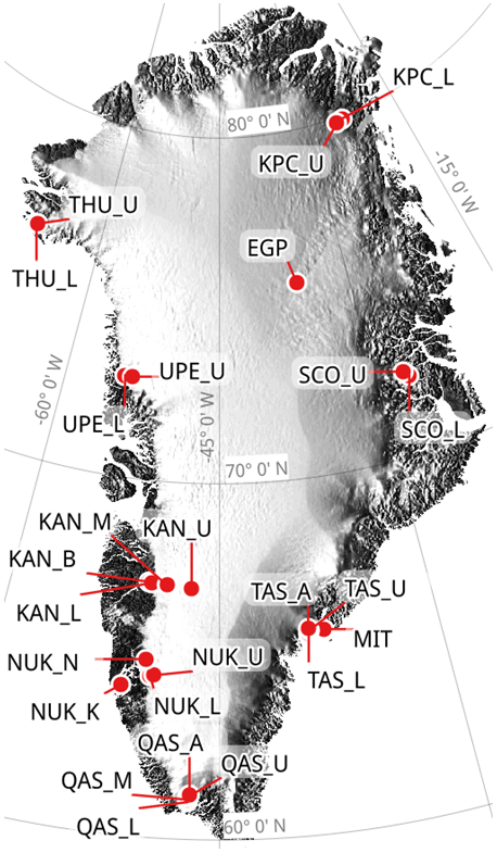
Figure 1Map of Greenland showing the PROMICE automatic weather station locations.
In 2007, the Programme for Monitoring of the Greenland Ice Sheet (PROMICE) was initiated (Ahlstrøm et al., 2008; van As et al., 2011b). GEUS developed rugged AWSs equipped with accurate instruments and placed them on the Greenland Ice Sheet as well as on local glaciers. The AWS design evolved over time with technological advances and lessons learnt, but the aim remained to obtain year-round, long-term, and accurate recordings of all variables of primary relevance to the surface mass and energy budgets of the ice sheet surface. The PROMICE monitoring sites were selected to best complement the spatial distribution of existing ice sheet weather stations, yet within range of heliports and airports.
The development of the PROMICE AWS started at GEUS in 2007 in collaboration with the GlacioBasis programme monitoring the A.P. Olsen Ice Cap in northeast Greenland (APO) and the Greenland Analogue Project in southwest Greenland. The AWS is designed to endure extreme temperatures and winds, countless frost cycles, and an ever-changing snow/ice surface while having dimensions and weight that allow for transportation by helicopter, snowmobile, or dogsled. The original PROMICE network consisted of 14 AWSs, with station pairs in seven regions: Kronprins Christian Land (KPC; Crown Prince Christian Land), Scoresbysund (SCO; Scoresby Sound), Tasiilaq (TAS), Qassimiut (QAS), Nuuk (NUK), Upernavik (UPE), and Thule (THU). Per region, the lower (L) station was placed near the ice sheet margin, and the upper (U) station was placed higher up in the ablation area, closer to or at the equilibrium line altitude (ELA) where long-term mass gains and losses are in balance (Fig. 1). Other projects collaborating with PROMICE led to the installation of 11 additional stations (Table 1). Currently, some regions also include stations at, for instance, middle (M) or bedrock (B) sites. Three PROMICE AWSs are located in the accumulation area of the ice sheet (KAN_U, CEN, and EGP), whereas two AWSs are on peripheral glaciers (NUK_K and MIT) not connected to the ice sheet. The PROMICE AWSs in Greenland transmit data by satellite in near-real time to support observational, remote sensing, and model studies; weather forecasting; local flight operations; as well as the planning of maintenance visits. The data have been important for quantifying ice sheet change in, for example, annual international assessment reports such as the Arctic Report Card 2020: Greenland Ice Sheet (Moon et al., 2020b) and the State of the Climate in 2019 (Moon et al., 2020a). The data have also proven crucial for calibrating, validating, and interpreting satellite-based observations and regional climate model output (Van As et al., 2014a; Noël et al., 2018; Huai et al., 2020; Kokhanovsky et al., 2020; Solgaard et al., 2021).
The aim of this paper is to describe the PROMICE AWS dataset in detail. We discuss the measurement with insights into post-processing and sensor calibration. The dataset is freely available at http://www.promice.org (last access: 5 February 2021, https://doi.org/10.22008/promice/data/aws). We start with a description on how to construct the AWSs, followed by a technical description of the AWS instruments, the data production chain, examples of typical station measurements, and finally a summary and outlook.
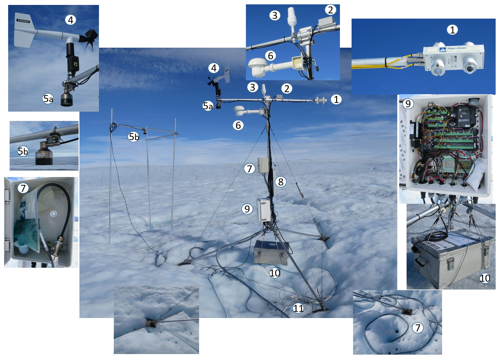
Figure 2PROMICE automatic weather station UPE_U photographed on 4 August 2018. The numbers shown in the figure denote the following: 1 – radiometer; 2 – inclinometer; 3 – satellite antenna; 4 – anemometer; 5 – sonic rangers; 6 – hygro-/thermometer (aspirated); 7 – pressure transducer; 8 – solar panel; 9 – data logger, multiplexer, barometer, satellite modem, and GPS antenna; 10 – battery box; 11 – thermistor string (eight levels).
2.1 The tripod
The AWS tripod is constructed from 32 mm (1.25′′) and 44 mm (1.75′′) radius aluminium tubes with 3 mm braided stainless-steel wires forming a free-standing tetrahedral structure that connects the legs and mast in a stable tripod (Fig. 2). Most sensors are attached to the 1.7 m long horizontal boom, which is 2.7 m above the surface (Fig. 2). Weighing ca. 50 kg, the battery box hangs under the mast to increase the mass of the AWS and to lower its centre of gravity for better stability (Table 1). The tripod can easily be folded to fit in small helicopters. The tripod can also be tilted during maintenance visit – for example, for sensor replacement. Because the tripod stands freely on the ice surface, it sinks with the melting surface, which results in sonic ranger measurements on the AWS that do not capture ice melt. Therefore, each PROMICE AWS on ice is accompanied by a separate sonic ranger stake assembly constructed from 32 mm aluminium tubing, typically drilled 7 m into the ice, that does not float on the ice (Fig. 2).
2.2 Instrumentation and data transmission
The PROMICE AWS measures (1) the meteorological parameters required for calculating the surface energy budget, (2) snow ablation/accumulation and ice ablation, (3) subsurface temperature at eight depths (thermistor string; Fig. 2), and (4) position by GPS. The next section provides details on the frequency and accuracy of measurements taken by each sensor. Further sensor details are provided in the Appendix.
Measurements are taken every 10 min and stored in the data logger locally. The AWSs transmit hourly averages based on 10 min measurements during the period with ample solar power, between day of the year 100 and 300 (10 April and 26 October in non-leap years). Exceptions are parameters with low variability (GPS position, station tilt, surface height, etc.) that are transmitted less frequently (every 6 h) in order to reduce the transmission cost. In winter, between day of the year 300 and 100, the stations only transmit daily averages of all parameters to limit power consumption by the satellite modem. Transmission is done through the Iridium satellite network that has coverage even at the northernmost latitudes. The Iridium Short Burst Data service transmits up to 340 bytes per message. The program running on the data logger ensures a correctly transferred data string from the logger to the transmitter if an Iridium satellite is in view. If the transmission through the satellite is not successful, the logger program will try again. Depending on the availability of the Iridium service, the logger program can also queue the message for delivery at a later time with better satellite connection. This relatively low-power operation mode ensures unnecessary transmission attempts with a low rate of message loss. Moreover, the logger program encodes the data in a binary format before transmission, which reduces the size of the message, thereby reducing transmission costs by about two-thirds.
To ensure reliable and accurate measurements, instruments in the field are swapped following an instrument maintenance schedule based on information from the manufacturers and from experience – for instance, the battery life and performance when charging batteries without a charge regulator. The maintenance schedule is only a guideline, and a field crew does not always return to an AWS in time to carry out a scheduled sensor swap. For example, the AWSs in the northeastern part of Greenland (KPC; Fig. 1) are only visited every 3–4 years, as their remoteness weighs heavily on the logistics budget. Thankfully, the most remote PROMICE AWSs experience less melt, lower accumulation, and weaker storms than some other places, reducing the need for maintenance visits. Maintenance visits typically take 2–4 h, which include replacing sensors scheduled for recalibration, re-drilling installed sensors in ice, and occasional repairs.

3.1 Dataset production chain
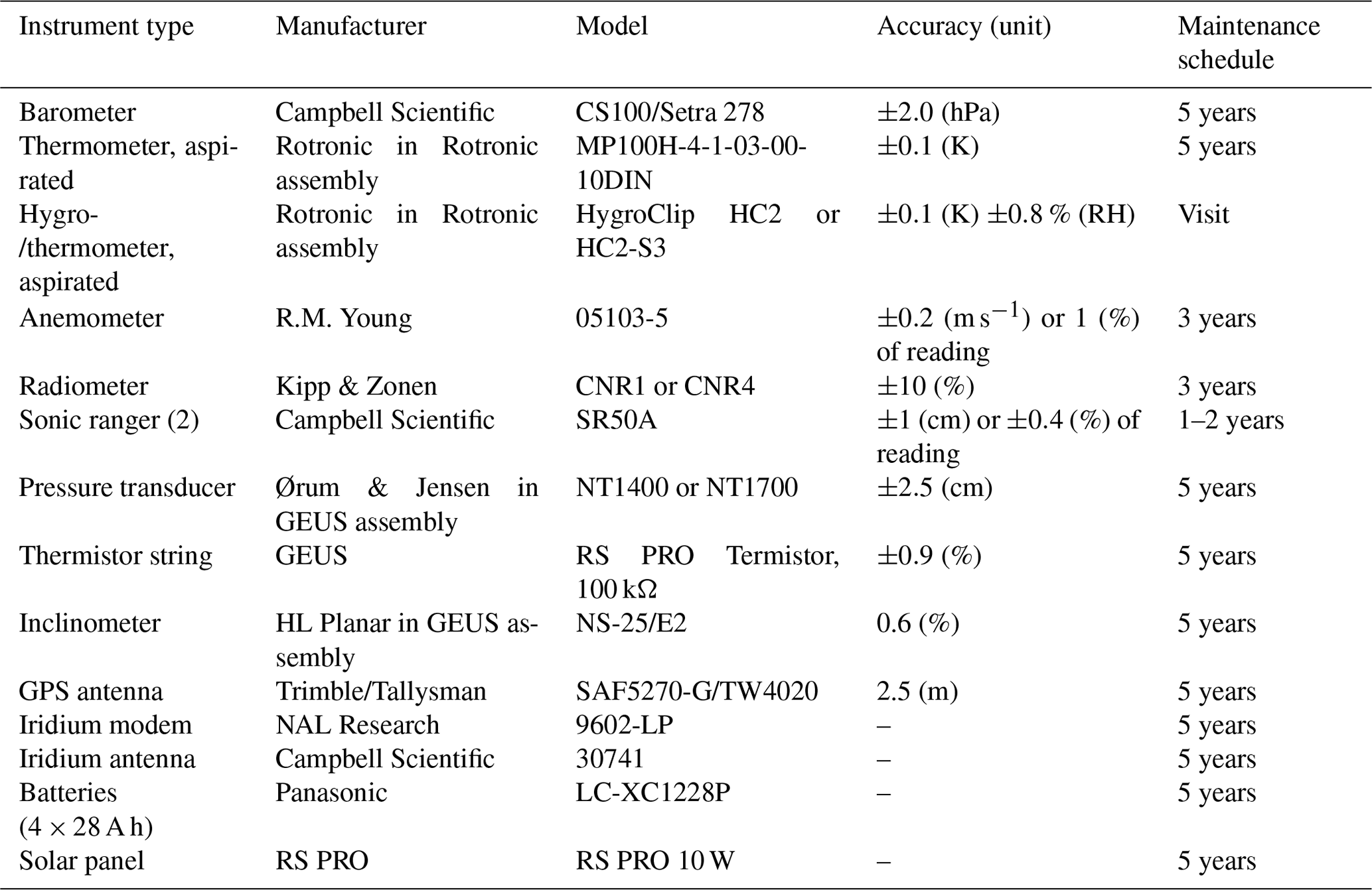
PROMICE AWS data are processed by the production chain algorithm with some manual expert quality checking twice a year (typically in January and after the summer); the data are also processed in real time with an automated quality check in the PROMICE database. For our production chain algorithm, we make use of the raw data recorded every 10 min, which are retrieved from the data logger during maintenance visits (Fig. 3). For the period since the last station visit, we use the transmitted data for the PROMICE data products. In addition to the direct AWS measurements, we also calculate certain variables based on these measurements, for instance tilt-corrected solar radiation and turbulent heat fluxes. In the following, we describe each variable in the PROMICE AWS dataset as well as how it is measured or derived. We refer to the manufacturer-specific instrument information, accuracy, and power consumption (see Table 2 and the sensor-specific tables in the Appendix). We use simple thresholds on 10 min data to remove spikes and inconsistent or bad measurements (see Sect. 3.3 below for more information). Available transmitted data are used for filling in data gaps.
Table 2Instrument information, accuracy, power, and maintenance schedule. More information on each instrument is available in Appendix A.
3.2 Measured variables: description and uncertainty
For most measured variables, the data logger converts readings in voltage to physical values using simple scaling relations with calibration coefficients specific for each instrument. Only when identical sensors can have different calibration coefficients, namely the radiometer and pressure transducer, is a conversion from voltage done in post-processing; the advantage of this is that a sensor swap does not require a data logger program change in the field. Below, we mention all scaling relations needed to manually convert logger data to physical measurements.
3.2.1 Air pressure
Barometric pressure (in hPa) is measured in the fibreglass-reinforced polyester logger enclosure (Fig. 2, number 9). The logger enclosure is generally located 1.5 m above the ice surface. The barometer manufacturer reports a measurement accuracy of ±2 hPa within the −40 to +60 ∘C temperature range (Table 2; see also the Appendix for more information).
3.2.2 Air temperature
Air temperature (in ∘C) is measured inside a fan-aspirated radiation shield (Fig. 2, number 6). The sensor is located approximately 2.6 m above the ice surface (i.e. as high as possible underneath the sensor boom). The measurement height varies when a winter snow cover is present. The temperature sensor is a PT100 probe that changes its electrical resistance with temperature and has an accuracy of ±0.1 ∘C (Table 2; see also the Appendix for more information). A secondary air temperature reading (in ∘C) is made in the aspirated shield from the HygroClip temperature/humidity sensor described in the following, which also has a manufacturer-stated accuracy of ±0.1 ∘C, but we consider the HygroClip temperature to be less accurate than the PT100, given the need for more frequent sensor recalibration.
3.2.3 Humidity
Relative humidity (RH; in %) is measured alongside the PT100 in the aspirated radiation shield using a HC2A-S3 (or HC2) HygroClip (Fig. 2, number 6). The sensor measures relative humidity with ±0.8 % accuracy. Relative humidity is measured relative to water. For temperatures below freezing, relative humidity is recalculated relative to ice in post-processing (see Sect. 3.3). To distinguish between the two relative humidities in the PROMICE data products, the prior humidity (unadjusted below freezing) is called “relative humidity with respect to water”, whereas the latter is simply referred to as “relative humidity”. The conversion of relative humidity relative to ice is after Goff and Gratch (1946). Every 1–2 years, the HygroClip is replaced by a sensor recalibrated in a closed chamber at room temperature with constant relative humidities of 10 %, 35 %, and 80 %.
3.2.4 Wind speed and direction
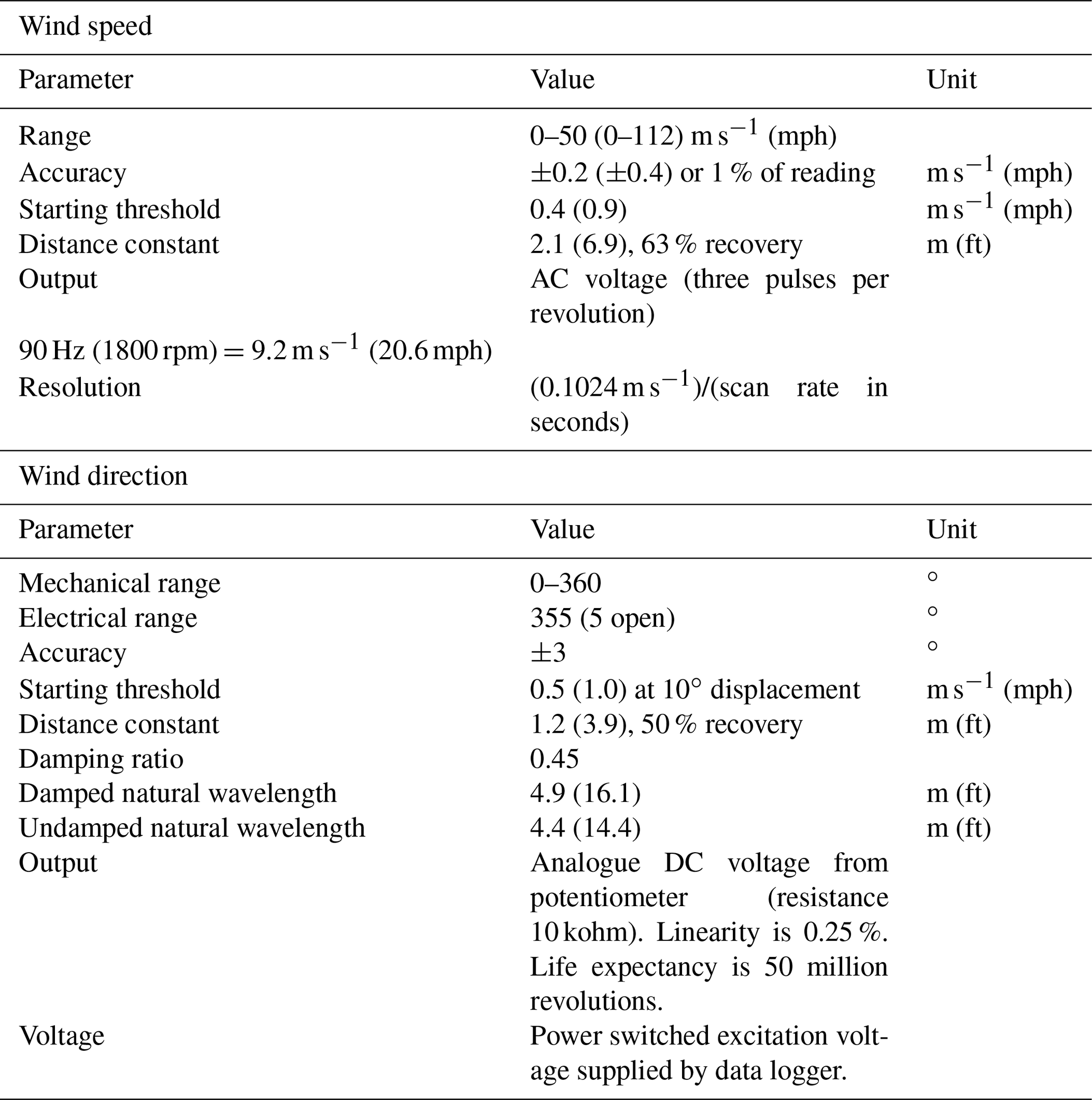
Wind speed and direction (in m s−1 and degrees respectively) measurement height is approximately 3.1 m above the ice surface and, like the other measurements, has a reduced measurement height if a winter snow layer is present (Fig. 2, number 4). An AC sine wave voltage signal is produced by the rotation of the four-bladed propeller, and the pulse count converts to wind speed using a multiplier. According to the manufacturer, the sensor can measure wind speeds between 0 and 100 m s−1, with an accuracy of ±0.3 m s−1 or 1 % if the measured value is higher than 30 m s−1.
Wind direction is measured through changes in the vane angle by a precision potentiometer housed in a sealed chamber on the instrument. The output voltage is directly proportional to vane angle wind direction and is measured between 0 and 360∘ with an accuracy of ±3∘. Every 3 years the sensor is replaced and tested for drift and functionality with an “anemometer drive” rotating the propeller at a known rate. The instrument's orientation is logged and reset to “geographic north” during each maintenance visit to keep wind direction data accurate within ±15∘ (although much larger station rotations have been encountered).
3.2.5 Upward and downward short-wave radiation
Horizontally levelled up- and down-facing Kipp & Zonen CNR1 or CNR4 record solar radiation (in W m−2) respectively. Measurement height is at the sensor boom level of 2.7 m over the ice surface (Fig. 2, number 1). Short-wave radiation is measured by the pyranometers within plastic meniscus domes, allowing minimal water droplet adhesion. The manufacturer reports that sensor uncertainty is 10 %. In practice, this sensor uncertainty has been found to be ca. 5 % for daily totals in Antarctica (van den Broeke et al., 2004). The radiometers are recalibrated at Kipp & Zonen every 3 years. The radiometer is one of the few variables stored in the data logger in voltage (V) units, because every radiometer has a different set of calibration coefficients, whereas all logger programs running on PROMICE AWSs are identical, for practical reasons. In post-processing, sensor readings SRraw are converted into a physical measurement SRm as follows:
where CSR (in V(W m−2)−1) is a sensor calibration coefficient, and SRm is either the converted downward or upward short-wave irradiance. Short-wave radiation measurements are corrected for sensor tilt following van As et al. (2011a) in post-processing, which means that the PROMICE AWS dataset contains both uncorrected and corrected values.
3.2.6 Upward and downward long-wave radiation
Long-wave radiation (in W m−2) is also measured by the CNR1/CNR4 radiometer mounted at approximately 2.7 m over the ice surface (Fig. 2, number 1). The radiometer contains a pair of up- and down-facing pyrgeometers, with a spectral range of 4.5 to 42 µm. In the same manner as for short-wave radiation, long-wave radiation is stored in voltage units (LRraw) in the data logger and transformed to physical units (LRm) in post-processing as follows:
where CLR (in V (W m−2)−1) is the sensor calibration coefficient, Trad is the sensor temperature measured in the radiometer casing (in ∘C), and T0=273.15 ∘C.
3.2.7 Surface height
The height of the sensor boom (in metres) is measured by a sonic ranger attached to the boom itself approximately 0.1 m below the boom (Fig. 2, number 5a), while the height of the stake assembly is measured about 0.1 m below an aluminium boom connecting stakes drilled into ice (Fig. 2, number 5b). The sensor outputs a distance (Hraw) that requires an air temperature correction in post-processing. The temperature adjustment is performed as follows:
After temperature correction, the measurement uncertainty of the SR50A sonic ranger reported by the manufacturer (Campbell Scientific) is ±1 cm or ±0.4 % of the measured distance. The uncertainty of sonic ranger readings in PROMICE was investigated utilizing data from a wintertime accumulation-free period of more than 2 months at the location SCO_U. The associated standard deviations for the two sensors were found to be 1.7 and 0.6 cm after spike removal, amounting to 0.7 % and 0.6 % of the measured distance respectively (Fausto et al., 2012). In addition to the sensor uncertainties, occasional problems with the stake assembly occurred, primarily in terms of stability during storms when melted out several metres. Also, an unknown amount of melt-in of the stake assembly can occur, but we speculate that this only happens (1) when surface melt since installation has been considerable, increasing the height and, thus, the pressure applied by the stake assembly, and (2) when the stake bottoms are not plugged with caps, as was only the case until 2010.
The PROMICE AWSs are also equipped with a pressure transducer assembly (PTA) that measures surface height change due to ice ablation (Fig. 2, number 7). The assembly was first constructed and implemented in Greenland in 2001 by Bøggild et al. (2004) but was further developed within PROMICE (Fausto et al., 2012). The PTA consists of a 50 / 50 antifreeze / water mixture-filled hose with a pressure transducer attached at the bottom. Drilling the hose typically more than 10 m into the ice, the pressure signal registered by the transducer will be that of the vertical liquid column over the sensor, where the upper level is a bladder fixed on the tripod in a shielded box. This allows inflow/outflow of antifreeze due to compression while keeping a steady level at roughly 1.5 m above the ice surface depending on the AWS. Figure 2 illustrates the free-standing AWS tripod that floats on the ice surface and moves down with the ablating surface, whereas the hose itself melts out of the ice, which, in turn, will reduce the hydrostatic pressure from the vertical liquid column over the pressure transducer at the bottom of the hose. The measured reduction in pressure at the bottom of the hose translates directly into ice ablation. As for the radiometer, every pressure transducer has a different calibration coefficient, which is why measurements are stored in the data logger in voltage units and transformed to a physical measurement in post-processing. Measurement height (Hm), or in fact depth relative to the PTA bladder, is calculated as follows:
where CPTA is the calibration coefficient. The constants ρw and ρaf are the densities of water and the 50 / 50 antifreeze / water solution respectively.
3.2.8 Subsurface temperature
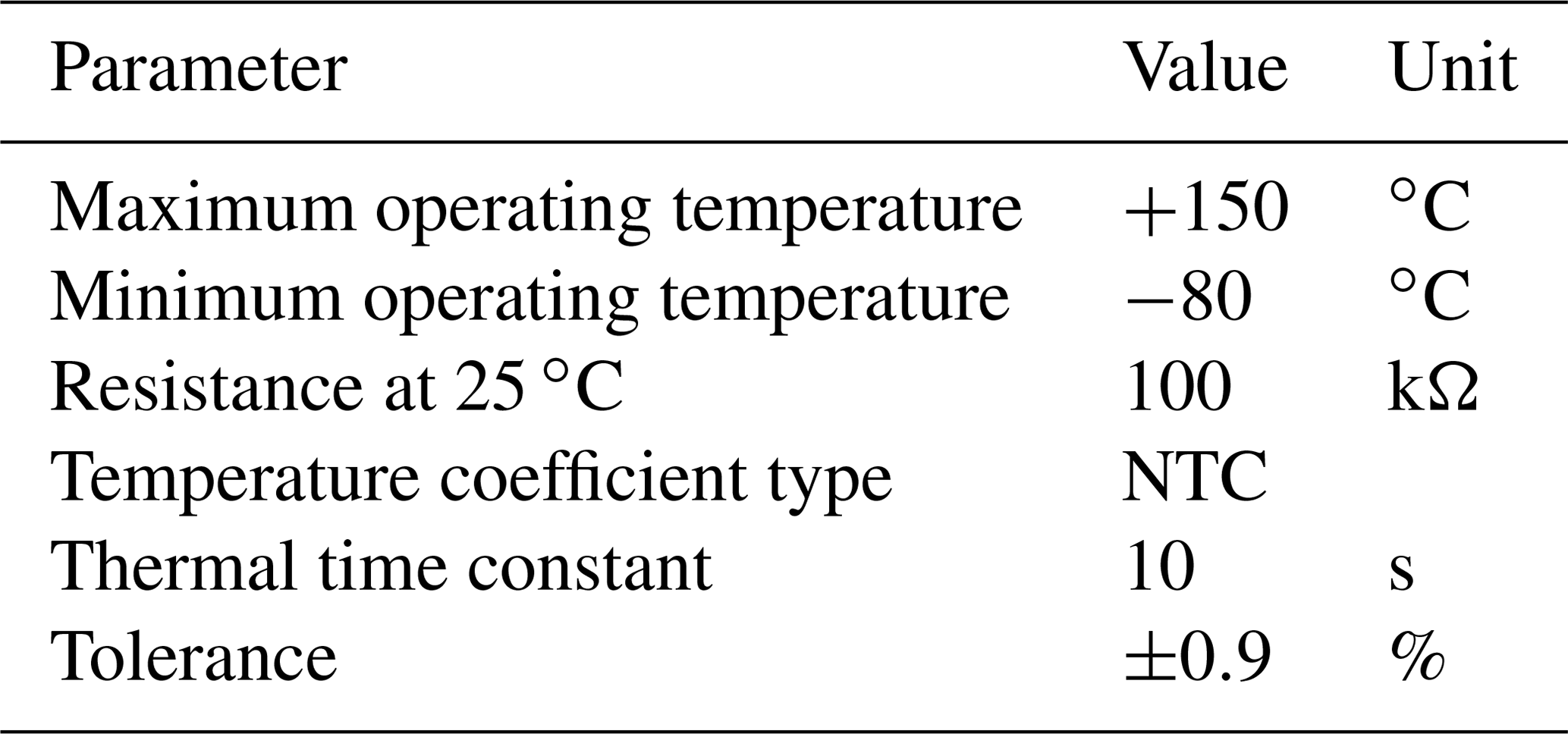
Subsurface temperatures (in ∘C) are measured by a 10 m thermistor (temperature-dependent resistor) string (Fig. 2, number 11). The string measures at 1, 2, 3, 4, 5, 6, 7, and 10 m depth, although depths vary due to the surface ablation and accumulation. The string is constructed at GEUS (see the Appendix for more information).
3.2.9 Station tilt
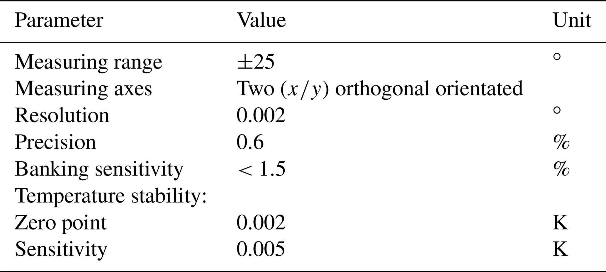
The inclinometer is installed on the sensor boom (Fig. 2, number 2) and is aligned with the radiometer to allow for tilt correction of short-wave radiation measurements. The inclinometer measures the tilt (in degrees) across (left–right) and along (up–down) the sensor boom, which translates into tilt-to-east and tilt-to-north when the sensor boom is perfectly oriented north–south. The tilt sensor readings in voltage units (Tiltraw) are converted into tilt in degrees as follows:
where all constants were determined at GEUS (Table 2). Ice ablation causes the AWS tripod to melt downward; this changing (slippery) surface often results in AWS tilt changes of more than several degrees.
3.2.10 AWS position
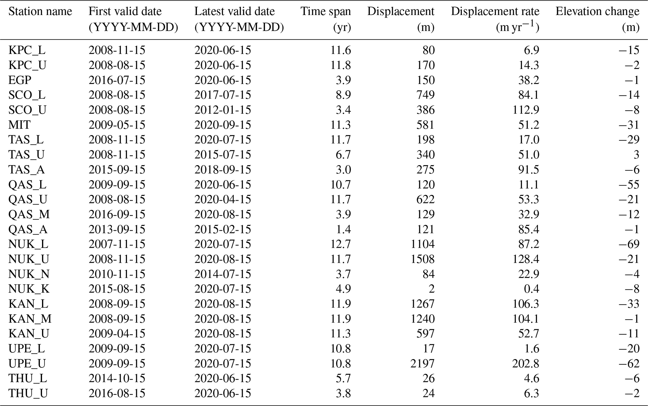
We use a single-frequency GPS receiver to measure the position (in ∘ N/∘ W) and the elevation (metres above sea level) of each station to quantify ice flow velocity (Fig. 2, number 9). The GPS antenna, as well as the receiver contained in the Iridium 9602-LP modem, is placed inside the data logger enclosure. The receiver type is described as follows: NEO-6Q, 1575.42 MHz (L1), 16-channel, and C/A code. The accuracy is reported to be within 2.5 m. In the PROMICE AWS set-up, the GPS receiver is powered up for 5 min preceding each Iridium transmission (hourly in summer and daily in winter), during which it attempts to acquire location data every 20 s. The return (out of a maximum of 15) that reports the lowest horizontal dilution of precision is written to memory. To date, NUK_U, NUK_L, MIT, and QAS_L have been repositioned during maintenance visits over distances larger than several tens of metres. The main reason for this is to reduce the influence of location change on the AWS variables measured, but stations have also been relocated to move them away from a region with opening crevasses. Table 4 shows the horizontal and vertical displacement due to glacier flow and AWS relocation during maintenance visits.
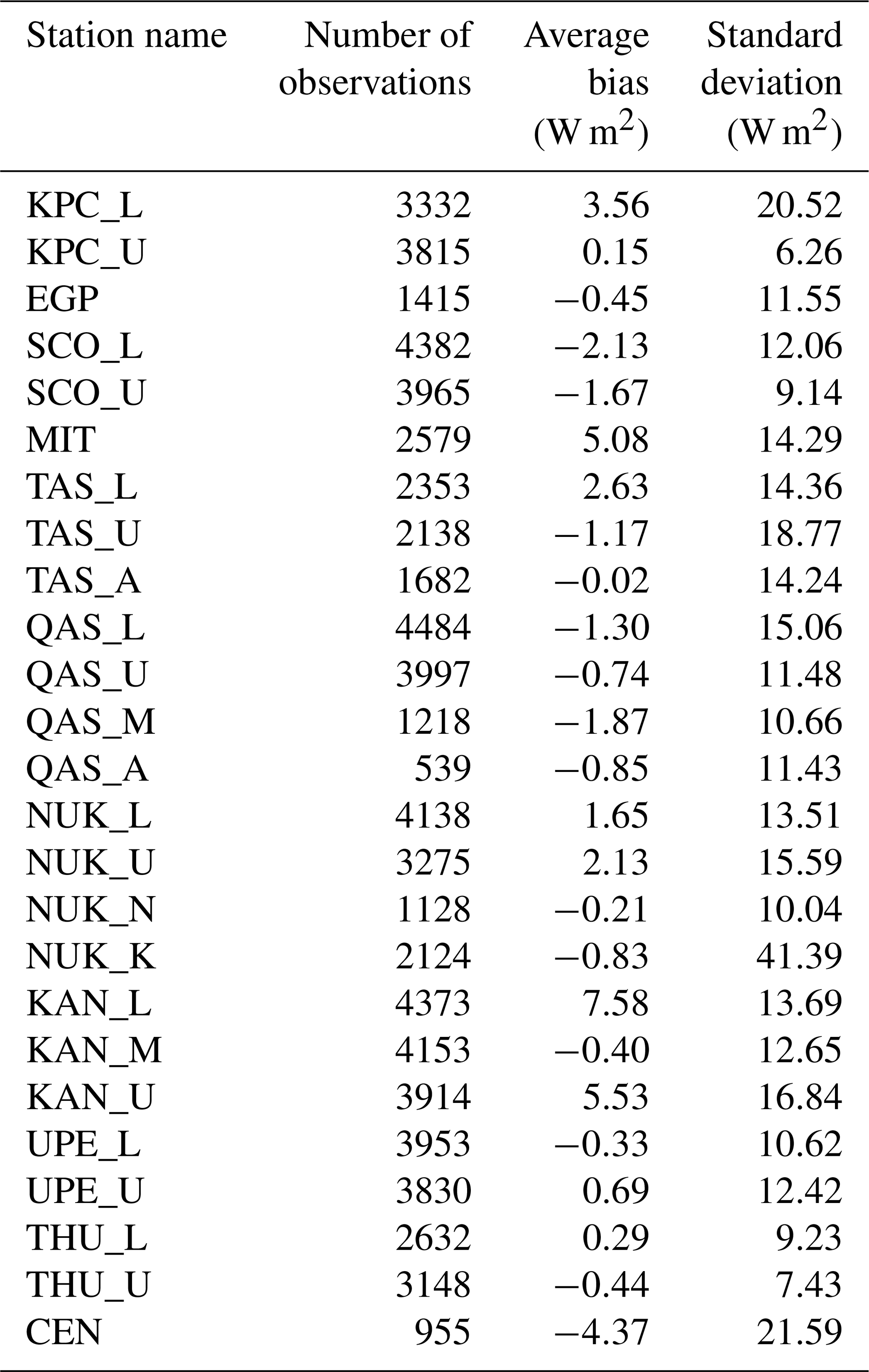
Table 3PROMICE AWS average bias and average standard deviation between corrected and uncorrected incoming solar radiation derived from the daily data product.
3.3 Post-processing
In this section, we describe and quantify the filtering process, how we correct measurements, and how we calculate derived variables in the dataset. The hourly, daily, and monthly averaging procedures are also described.
Table 4PROMICE AWS displacement statistics from monthly average GPS data. There are no GPS data available for AWS CEN.
3.3.1 Filtering
Table 5 provides filtering information used in the processing chain. We remove unrealistic spikes from the data by using upper and lower thresholds for each measurement. Measurements outside these (generous) threshold limits, which could occur for a number of known and unknown reasons, are considered erroneous and set to −999. Known reasons will be discussed in Sect. 4.3 (living data section). Derived variables are also set to −999 when one or more of the listed “core” AWS measurements that serve as input fall outside the threshold limits.
3.3.2 Derived and corrected variables
Specific humidity
The specific humidity q (in kg kg−1) is calculated from relative humidity with respect to water/ice above/below freezing (RH) using the following equation:
with
where ϵ=0.622 is the ratio between the specific gas constants for dry air and water vapour, p is air pressure (in Pa), and is saturation water vapour pressure (in Pa) over ice (below freezing) or water (above freezing) calculated after Goff and Gratch (1946).
Surface temperature
The surface temperature Ts (in ∘C) is derived using the measured downward and upward long-wave irradiance (LRin and LRout respectively):
where ice sheet surface emissivity ϵ=0.97.
Turbulent energy fluxes
The sensible and latent heat fluxes (SHF and LHF respectively; in W m−2) are estimated using vertical gradients in wind speed, potential temperature, and specific humidity between the measured boom height and the surface described by Van As et al. (2005) and Van As (2011). According to the Monin–Obukhov similarity theory, SHF and LHF can be approximated as follows:
Here, ρ is the density of air, and Cp=1005 is the specific heat capacity at constant pressure. J kg−1 and J kg−1 are the latent heat values of sublimation and evaporation respectively, and κ=0.4 is the von Kármán constant. When estimating turbulent heat fluxes, we need the measurement heights (zu, zT, zq; Table 2) of wind speed (u), temperature (T), and specific humidity (q) as well as the surface roughness lengths for momentum z0, for heat z0,T, and for moisture z0,q. We use z0=0.001 m, and is calculated using the formulation from Smeets and Van den Broeke (2008a, b) for rough surfaces. We use the stability correction functions from Eq. (12) in Holtslag and De Bruin (1988) for stable atmospheric conditions, and we follow Paulson (1970) for unstable conditions. The surface temperature (Ts) is calculated from long-wave radiation (see Eq. 8), and the surface specific humidity is assumed to be at saturation (qs=qsat).
Several sources of uncertainty apply to the calculation of SHF and LHF. The aerodynamic surface roughness length z0 is known to vary with surface type (Brock et al., 2006) and through time (Smeets and Van den Broeke, 2008a, b). Using the constant value of z0=0.001 m could be an overestimation of surface roughness in the presence of snow and could subsequently lead to an overestimation of both turbulent fluxes. As most PROMICE stations are located in the ablation area, the snowpack is melted during spring and the surface becomes snow-free for most of the ablation season. The calculation of surface temperature also relies on certain assumptions (see the section above). Several studies have evaluated the performance of the Monin–Obukhov similarity theory in Greenland. Using one- and two-level methods vs. eddy covariance and evaporation lysimeters, Box and Steffen (2001) found an underestimation of downward LHF during extreme stability cases. Miller et al. (2017) used a similar method for calculating SHF and reported a root-mean-square difference (RMSD) of 8.7 W m−2, with an average bias of −7.0 W m−2, when compared with their two-level eddy-covariance estimation of SHF. Miller et al. (2017) emphasized that SHF records from one-level approaches often cover longer time periods. Fausto et al. (2016a, b) investigated the use of an unrealistically high z0 to get agreement between surface energy balance (SEB) closure and observed ablation rates during extreme sensible and latent heat-driven melt events.
Tilt correction of downward short-wave radiation and cloud cover
Tilt correction of solar radiation is performed following Van As (2011). Downward short-wave radiation (SRin) consists of a diffuse and direct beam part. It is only the direct beam part of SRin that requires tilt correction. For a horizontal radiation sensor, the direct beam, which equals SRin, is reduced by its diffuse fraction (fdif). For the tilted radiation sensor, SRin is calculated from the measured value, SRin,m, and a correction factor, C, as follows:
with
where SZA is the solar zenith angle, d is the sun declination (the angle of the sun above the plane formed by the Earth's Equator), w is the hour angle (the angle between the sun's current position in the sky and its position at solar noon), lat is the site's respective latitude in radians, and θsensor and ϕsensor are the radiometer's tilt angle and direction respectively. The calculation procedures for d, w, and SZA are detailed in Vignola (2019). Table 3 illustrates the average bias or correction made for the incoming solar radiation based on Eq. (11). The standard deviation indicates that the average correction is minor (below 15 W m−2) for most AWSs, whereas a few AWSs have corrections values spread out over a wider range.
Table 5Threshold values used in the filtering process for each measured variable.

We estimate fdif spanning from 0.2 for clear skies to 1 for overcast conditions, while assuming a linear dependency on the cloud cover fraction (Harrison et al., 2008). We approximate the cloud cover fraction from the dependence of the near-surface air temperature (Tair) on LRin (Van As et al., 2005). For this purpose, we calculate a theoretical downward long-wave radiation flux corresponding to clear-sky conditions using the equation from Swinbank (1963):
We calculate a theoretical downward long-wave radiation flux corresponding to overcast conditions assuming the black-body radiation as follows:
The cloud cover (limited to the [0:1] range) is then calculated as
Albedo
Surface broadband solar reflectivity in the 0.3 to 2.5 µm wavelength range, also known as albedo (unitless), is calculated from 10 min tilt-corrected downward and upward solar irradiance data. Hourly averaged albedo values are calculated for cases when the sun hits the radiometer top at angles exceeding 20∘ (i.e. when measurements are most reliable for this sensor type). Daily albedo averages are computed from available hourly data. AWS obstruction of sunlight, casting a shadow within the radiometer's field of view, may lower the albedo on average by 0.03 (Kokhanovsky et al., 2020), but this depends on the surface type and height. Also of relevance to measured albedo is the contrast of the surface relative to the AWS battery box, legs, mast, and enclosure, as well as whether a melt pond forms beneath the AWS. Ryan et al. (2017) examined spatial variograms in unoccupied-aerial-vehicle-derived albedo vs. satellite and PROMICE albedo and found increasing differences for some PROMICE sites toward the late melt season when the AWS point measurements lack representativity of the increasingly inhomogeneous surface cover. A study by van den Broeke et al. (2004) found a 5 % uncertainty on pyranometer measurements, although the manufacturer, Kipp & Zonen, estimates a more conservative value of 10 % uncertainty. We conservatively assume 10 % uncertainty in the calculated albedo.
Ice surface height
The pressure transducer assembly (PTA; Fig. 2, sensor 7) set-up is influenced by variations in air pressure. The air pressure contributions to the measured PTA signal HM are eliminated using the following equation:
where PA (in hPa) is air pressure, PC (in hPa) is the known pressure given by the manufacturer to which the sensor was calibrated, g=9.82 m s−2 is the gravitational acceleration, and ρl=1090 kg m−3 is the antifreeze mixture density at 0 ∘C. Changes in HL are equal to ice ablation. Fausto et al. (2012, 2016a) compared PTA time series to hose measurements manually performed in the field and recorded distances from sonic rangers to quantify instrument inaccuracies, which were found to be accurate to within 0.04 m.
3.3.3 Averaging
The time reported in our data products specifies the hour/day/month during which the measurements are taken, as opposed to other products that list the exact timestamp of the end of the averaging period. Hourly averages are calculated from 10 min values if at least one value is available (10 min data are seldom missing). We then calculate daily averages from hourly averages if at least 20 values (∼80 %) are available for a dataset variables with a clear diurnal variability. Less transient variables require at least one measurement to calculate an average. Lastly, we calculate the monthly averages from daily averages if at least 24 values (∼80 %) are available.
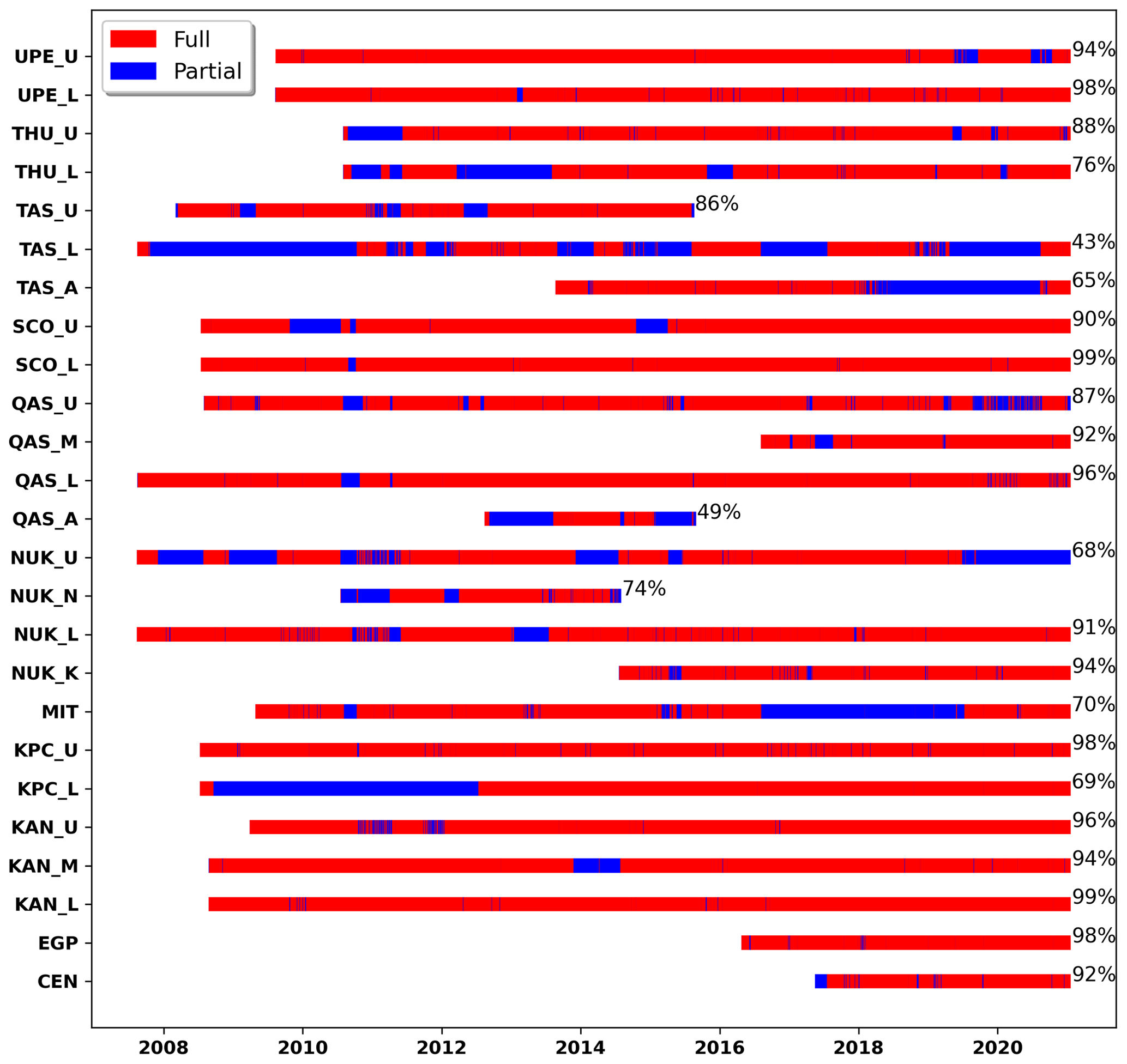
Figure 4Combined availability of the eight critical variables required for surface energy balance calculation from PROMICE daily products. See the Appendix for the data availability of each of the variables.
3.3.4 Measurement success rate
To illustrate the PROMICE AWS data coverage, we determined the “success rate” in terms of available daily averages for all measured variables that are required for estimating the surface energy budget: air pressure, air temperature, humidity, wind speed, and downward and upward short-wave and long-wave radiation. Success rate is defined as the ratio of the counts of successful variable estimate and the number of days since AWS installation. The performance for the critical variables for each station and their measurement periods are illustrated in Fig. 4. A total of 18 of the 26 stations have at least an 85 % success rate for all critical surface energy budget variables, while 6 have experienced significant periods with power failure, station toppling, snow accumulation exceeding the instrument height, or even crevasse formation underneath the station.
Table 6Short description of all the variables in our data products. An updated version of this short description is kept as a README.txt file in the data product download folder.
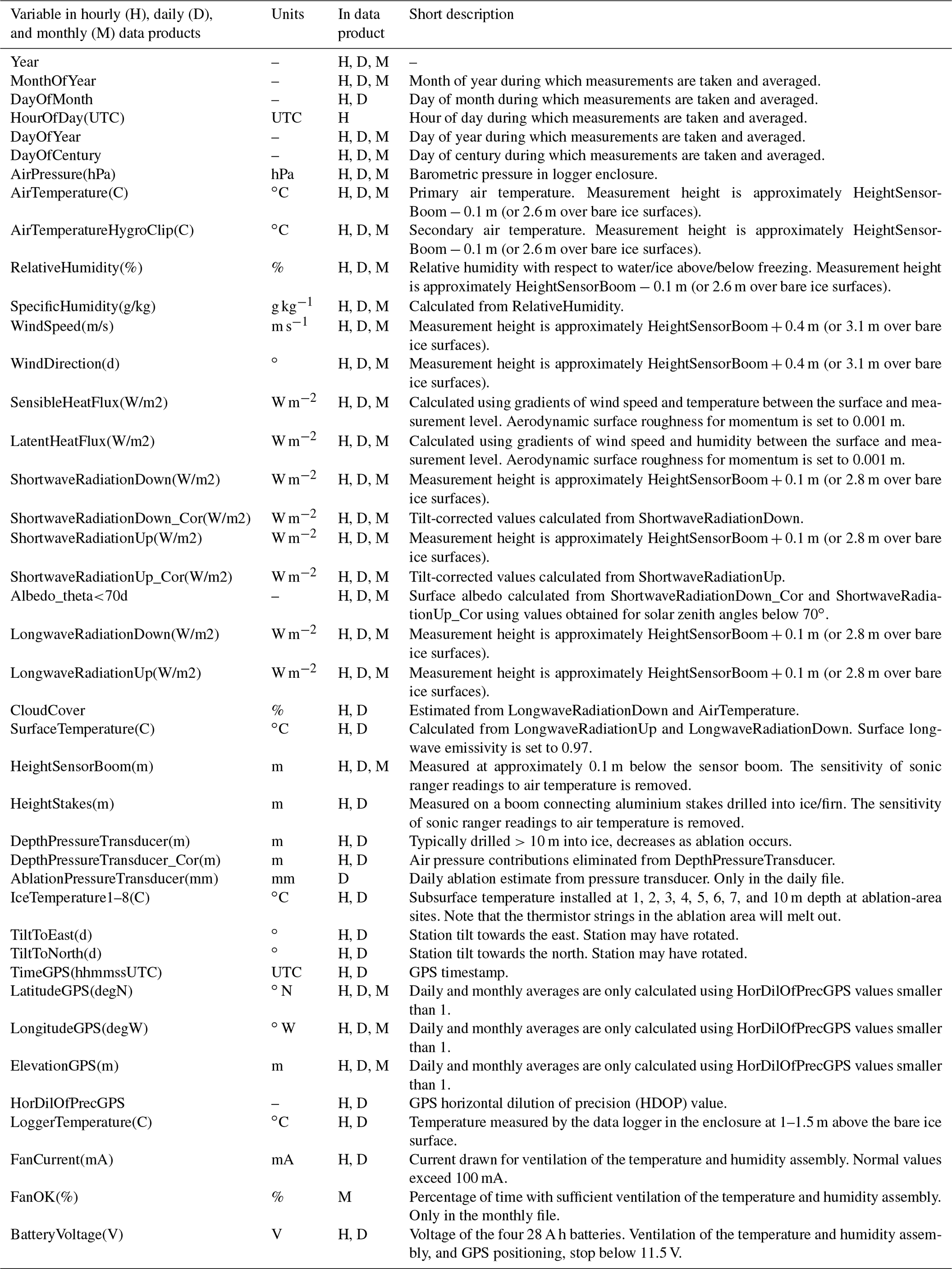
The PROMICE AWS data are made available at hourly (H), daily (D), and monthly (M) time resolutions. The data products include the variables listed in Table 6. The data are organized in ASCII files, following Table 6, with 46 columns in the hourly data files, 45 columns in the daily data files, and 24 columns in the monthly data files. The data files can be accessed via “Download Data” on the PROMICE website: https://www.promice.org (last access: 5 February 2021, DOI: https://doi.org/10.22008/promice/data/aws).
4.1 Data climatology: average and standard deviation
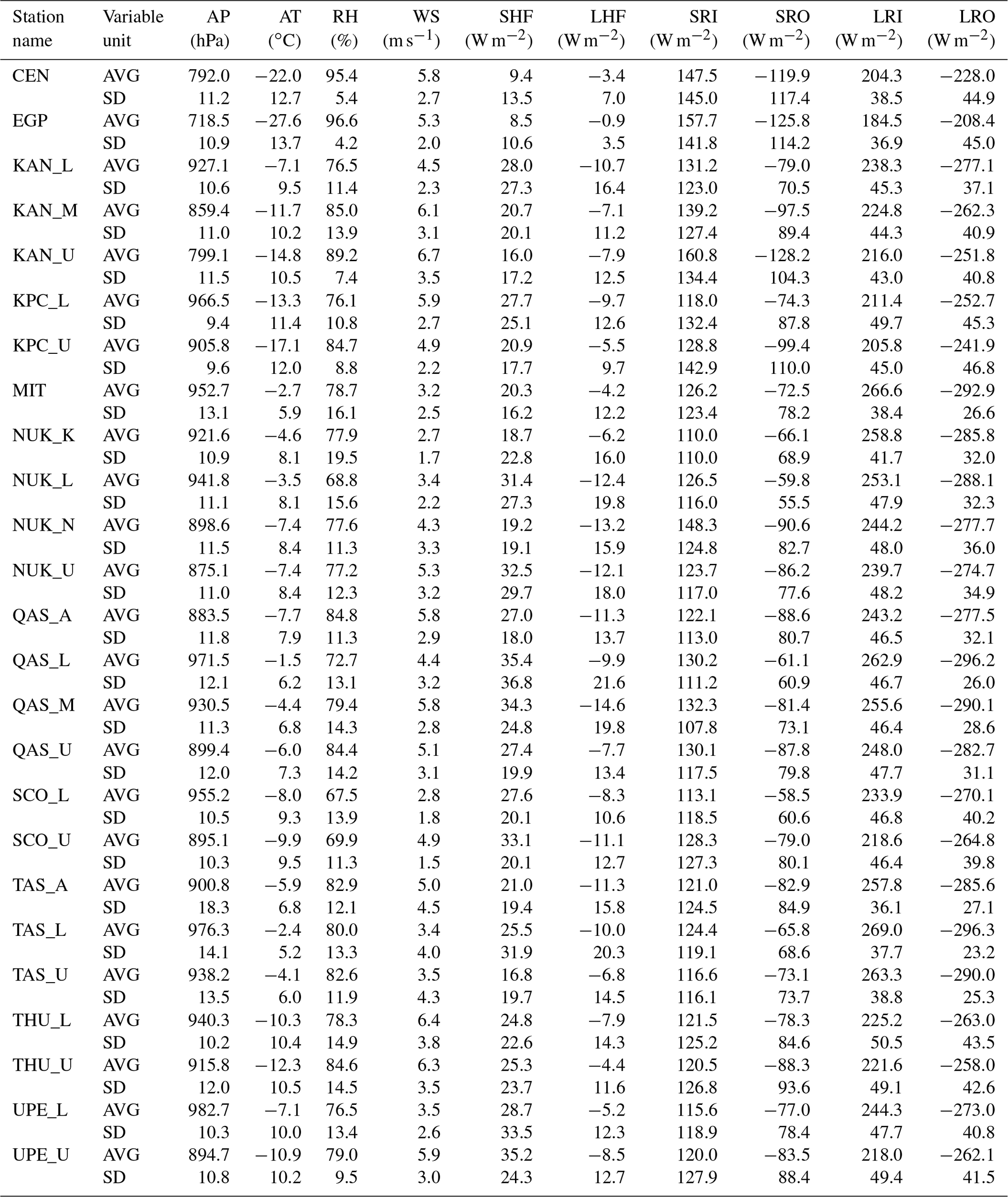
Here, we briefly present the meteorological variables and the surface energy balance components based on the daily data product. Table B1 shows the average and standard deviation for all available dataset variables for the 2008–2020 period. In general, Table B1 illustrates that the short-wave radiative fluxes vary from 118.0±134.2 at KPC_L in the north to 130.2±111.2 at QAS_L in the south depending mainly on cloud cover and season. Stations at higher elevation tend to get more sunlight than the lower-lying stations (van As et al., 2013; Fausto et al., 2016b). The turbulent fluxes (sensible and latent heat) show a positive contribution from the sensible heat flux and a negative contribution from the latent heat flux, both with a considerable variation. The turbulent fluxes are on average lower in magnitude than the radiative fluxes and tend to be higher at lower latitudes and elevation (Fausto et al., 2016b). The temperature is generally higher for stations located at lower elevations close to the ice sheet margin, as they are more exposed to the relatively warm atmospheric conditions of the ocean all year round, except for stations at higher latitudes (above 70∘ N) which experience sea ice conditions during winter that influence the temperature (van As et al., 2011a, 2014b). Table B1 also illustrates that the temperature has a clear dependence on latitude and elevation. On average, the wind speed tends to increase with elevation, which is mainly due to the surface radiative cooling during winter (van As et al., 2014b).
4.2 Data examples
To create a quick insight into the data product, we show examples of data from AWSs in two contrasting locations: TAS in southeast Greenland near Tasiilaq and UPE in northwest Greenland near Upernavik (Fig. 1).

4.2.1 Wind speed
Time series spanning the years 2012 through 2014 of weekly median wind speeds and maximum 10 min wind speed within that week for TAS_L and UPE_U are displayed in Fig. 5. Median wind speeds are lower at TAS_L than at UPE_U, whereas the opposite is true for maximum wind speeds because TAS_L is located in a region well-known for its piteraq storms.
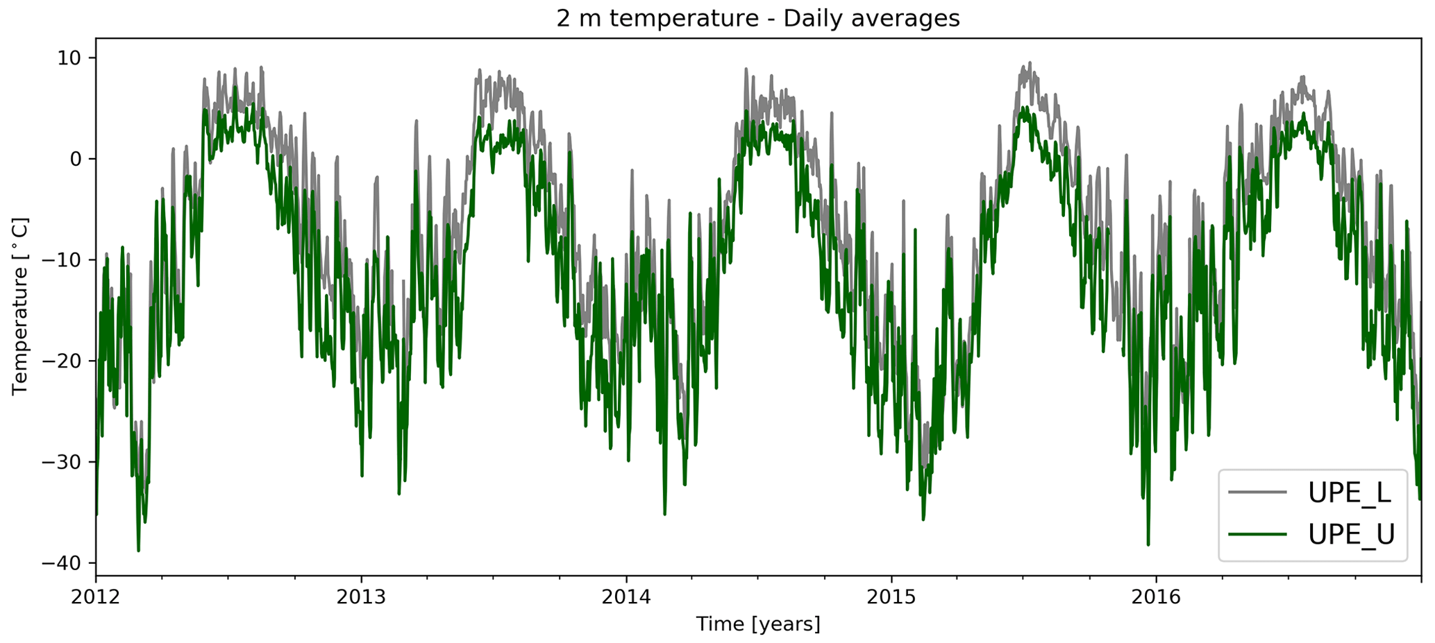
4.2.2 Air temperature
The daily average air temperature for the two stations near Upernavik is shown in Fig. 6. The temperature is higher at the lower station, UPE_L, than at the upper station, UPE_U, due to an elevation difference of more than 700 m. The tendency of the temperature to have a higher variability during winter months than during summer is also evident from these time series.

4.2.3 Surface energy balance
Figure 7 presents the surface energy fluxes at UPE_U in 2012. The plots show how UPE_U experiences a shorter period with solar radiation, due to the more northerly location, when comparing it to the TAS stations further south. Furthermore, Fig. 7 shows how the outgoing long-wave radiation becomes stable during the main melt season when the surface temperature is at the melting point. The sum of all the fluxes determines if there is a surplus of energy at the surface, which can be used for snow or ice melt.
4.3 Living data and continuing improvements
PROMICE will continue to update and provide the data products as AWS data comes in. It is likely that there are currently unknown issues in the existing data released as part of this dataset, and new issues may arise in data collected in the future. Moreover, some issues are known but are hard to identify, and some issues are systematic, which can be corrected for more generally. Below, we list known dataset issues in three categories: (1) issues that are hard to identify, (2) issues that we can systematically correct for in some way, and (3) errors caused by humans, animals, and instrument failure.
Here, we list dataset issues that we have encountered over the years following the above three categories:
-
Hard to identify
-
high inclinometer variability, presumably caused by AWS shaking, or instrument failure;
-
riming affecting several measured variables;
-
undocumented AWS orientational drift;
-
sonic ranger membrane not robust enough to consistently survive the period between maintenance visits (instrument failure);
-
instruments buried in snow during winter and/or spring;
-
tripod collapse due to compacting snow;
-
AWS falling over in extreme winds or crevassed terrain;
-
bent sensor boom due to compacting snow, impacting the alignment radiometer and inclinometer;
-
leaks in or overfilling of the pressure transducer assembly;
-
static electricity by snow drift or damage to the AWS’s electrical circuit.
-
-
Systematic correction
-
radiometer sensor tilt (already corrected for);
-
glacial movement causing gradual changes in AWS positions and, thus, their measured variables
-
shading by instruments and station frame impacting measurements (e.g. albedo).
-
-
Errors caused by humans and animals
-
human error, such as sensor plug swap during maintenance visits or improper (incorrect height/orientation) sensor mounting;
-
animal occasionally soiling instruments and AWS surroundings;
-
various instrument failures.
-
The most recent data files will, in most cases, be comprised of transmitted data, which will be updated after the next maintenance visit. Data download from the logger will improve data quality and coverage. During strong winds, the AWSs can topple or sensors can break down. AWSs can also be covered by snow that accumulates in winter, which reduces the data quality for many variables. Using our height measurements on both the station and the stake assembly, we can monitor when certain instruments are covered in snow. At present, AWSs being covered in snow has only occurred at three locations, namely QAS_U, QAS_M, and MIT. Data recorded after and during these events are often identified by the automatic processing routine and will be clearly identifiable for the data user as erroneous data. A maintenance visit either in spring or summer will often result in a station being moved, levelled, and/or rotated, in which case variables such as surface height will undergo an easily recognizable shift.
The following are identified dataset issues that we plan to correct for or implement in future data products:
-
shading by instruments and station frame impacting albedo;
-
instrumental monitoring of AWS orientation, which could influence the correction of the short-wave radiation and wind direction;
-
instrumental monitoring of rain;
-
flagging protocol for identified errors and issues.
While we do our best to clean the data appropriately and address known issues (see above), we recognize that correcting issues is more complicated than simply documenting them and that some corrections may not be possible or may be subjective and a function of different use cases. Therefore, we introduce a user-contributable dynamic web-based database of known data quality issues at https://github.com/GEUS-Glaciology-and-Climate/PROMICE-AWS-data-issues/ (last access: 7 April 2021). The current implementation uses GitHub “issues”, although a future version may use a different database at the back end that the DOI would resolve. Each issue is tagged with station(s), sensor(s), and year(s) where the issue occurs. Users who are working with a station, sensor, or time frame of data are encouraged to search the issue database and see if there are any known relevant data issues. If users discover a data issue that is not currently documented, they can add it to the database. A PROMICE team member will review and tag any issues as verified and then suggest a fix. Future versions of the product will implement these fixes if possible, and the issues will be closed but remain accessible.
The PROMICE AWS product is available from https://doi.org/10.22008/promice/data/aws (Fausto et al., 2019).
The processing code is available at https://doi.org/10.22008/W19C-B256 (van As et al., 2021).
The UN Intergovernmental Panel on Climate Change (IPCC) has previously highlighted the value of station-level records for assessing the cryospheric changes associated with global climate change (Vaughan et al., 2013). The IPCC has more recently highlighted the importance of understanding Greenland Ice Sheet mass loss, especially mass loss due to atmospheric forcing and surface mass balance mechanisms, as a leading contributor to sea level rise (Meredith et al., 2019). Meteorological and glaciological monitoring sites on the ice sheet are necessary to provide well-constrained observations of surface energy and mass balances. Understanding these local energy and mass balances provides the process-level knowledge of ice sheet and atmosphere interactions required by regional and global simulations (e.g. Van As, 2011; Fausto et al., 2016b). The PROMICE network plays a leading role in providing these in situ observations and process-level insights for the Greenland Ice Sheet.
The PROMICE AWS v3 data products are made available as hourly, daily, and monthly data files. All data products undergo periodical improvement through updates in the processing chain. Data are added as they are received from field parties and via satellite transmission. Between 2007 and 2021, the PROMICE AWSs have carried out measurements with an 85 % success rate for 18 of the 26 stations, defined as the availability fraction of the daily averages for variables required for calculating the surface energy balance (see Fig. 4). All PROMICE AWS data products are available at https://doi.org/10.22008/promice/data/aws.
In addition to advancing science, the PROMICE AWS network is now poised to contribute to operational products. With recent advances in the quality and transparency of the PROMICE data delivery pipeline described here, as well as the increasing prevalence of machine-to-machine transfer protocols among data users, the entire PROMICE station data archive – including near-real-time observations – is now readily available to ingest in weather forecast and climate reanalysis applications. With the original AWS stations quickly approaching their 15th anniversary, the PROMICE data record is crossing the halfway mark of a 30-year climatological reference period. With the launch of the PROMICE AWS data issues on GitHub (https://github.com/GEUS-Glaciology-and-Climate/PROMICE-AWS-data-issues/, last access: 7 April 2021), we hope to continue to support the growing PROMICE user community into the next decade.
A1 Instrument information, accuracy, and power consumption
A1.1 Barometer
Table A1Barometer: details from the manufacturer for the Setra CS100 barometric pressure sensor (model 278).

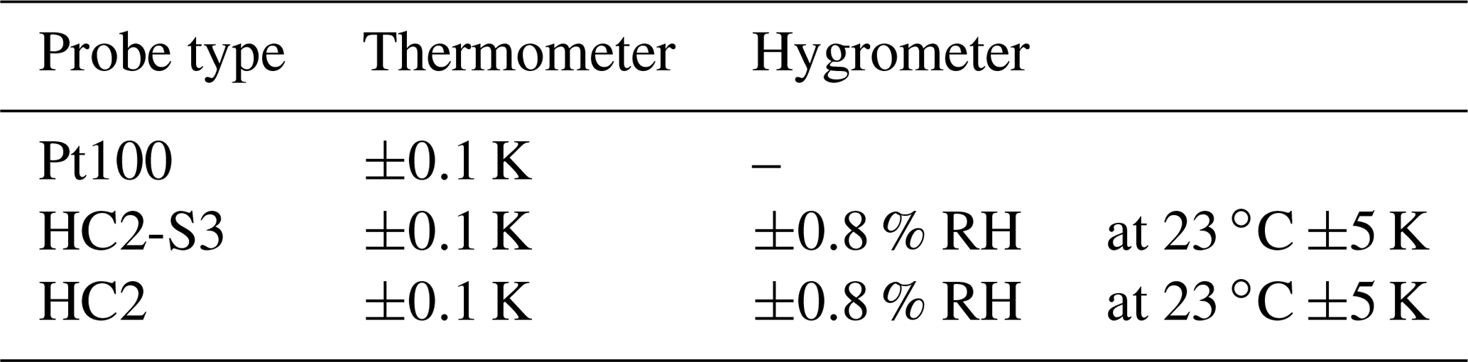
A1.2 Thermometer and hygrometer
Rotronic MP102H with a Pt100 (±0.1 K) and HC2-S3 (or HC2) probe (±0.1 K, ±0.8 % RH, at 23 ∘C ±5 K), housed in an RS12T aspirated shield. The Rotronic system uses ventilated weather and radiation shields: RS12T with a 12 V DC fan. Due to the white housing of the radiation shield, the influence of thermal radiation on the measurements of temperature and humidity is reduced to a minimum. The shield also offers optimum protection in stormy weather, even against horizontally driven rain and snow. The fan is supplied by a separate cable.
Table A2Thermometer and hygrometer: details from the manufacturer Rotronic.
A1.3 Anemometer
Table A3Anemometer: details from the manufacturer Young (model 05103).
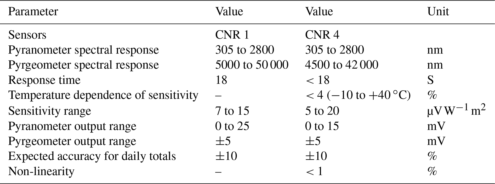
A1.4 Radiometer
The radiometers used were Kipp & Zonen CNR1 and CNR4 instruments. CNR4 is a four-component net radiometer for accurate and reliable measurements. There are four separate signal outputs, and the integrated temperature sensors can be used to calculate the net radiation. The CNR4 combines two pyranometers for solar radiation with two pyrgeometers for infrared measurements. The upper pyrgeometer has a silicon meniscus dome so that water rolls off, and the field of view is 180∘. The design is lightweight, and the white sun shield reduces solar heating of the instrument body. Although similar to CNR4, the older CNR1 has a slightly different instrument body and measurement range (see the tables below) but performs with similar accuracy. We do not flag the products with respect to which instrument type we used for that each station set-up. Therefore, we assume the same accuracy for both the CNR1 and CNR4.
Table A4Thermometer and hygrometer: details from the manufacturer Rotronic.
A1.5 Thermistor
Table A5Thermistor: details from the manufacturer; fabricated at GEUS – the thermistor strings are based on resistors. NTC denotes the negative temperature coefficient.
A1.6 Inclinometer
Table A6Inclinometer: details from the manufacturer HL Planartechnik (model NS-25/E2).
A1.7 Sonic rangers
The accuracy of the SR50A sonic ranger given by the manufacturer (Campbell Scientific) is ±1 cm or ±0.4 % of the measuring height after temperature correction.
A1.8 Pressure transducer
The PROMICE AWSs are equipped with an Ørum & Jensen NT1400/NT1700 pressure transducer assembly (PTA). The PTA monitors ice surface height change due to ablation. The pressure transducer sensor has an accuracy of 2.5 cm given by the manufacturer.
A1.9 GPS
We have equipped a single-frequency GPS. It is built into an Iridium 9602-LP modem. The manufacturer describes the receiver type in the following way: NEO-6Q, 1575.42 MHz (L1), 16-channel, C/A code; accuracy of 2.5 m CEP (circular error probable); update rate of 5 Hz; start-up times of 1 s for hot starts and 28 s for warm starts and cold starts; sensitivity of −160 dBm.
Table B1Average (AVG) and standard deviation (SD) for metrological variables and surface energy balance components derived from the daily products: air pressure (AP), air temperature (AT), relative humidity (RH), wind speed (WS), sensible heat flux (SHF), latent heat flux (LHF), incoming solar radiation (SRI), outgoing solar radiation (SRO), incoming long-wave radiation (LRI), and outgoing long-wave radiation (LRO). The sign convention is as follows: negative fluxes remove energy from the surface, whereas positive fluxes add energy to the surface. This table supplements Fig. 4.
AA, SA, DvA, and RF designed, managed, and received funding for the PROMICE monitoring programme for the 2007–2021 period. RF and DvA produced the PROMICE AWS product. RF and KM set up the data curation framework. MC, AP, CS, RF, and DvA contributed to the sensor and AWS design. SN also contributed to the sensor and AWS design but passed away before submission; we regard their approval of this work as implicit. RF, BV, JB, WC, and KM contributed to the data analysis and validation. RF, AS, SL, NK, KK, NK, and JB were responsible for the data product description, data climatology, and data examples. All authors carried out the data assimilation. RF prepared the paper with contributions from all co-authors.
The authors declare that they have no conflict of interest.
Publisher's note: Copernicus Publications remains neutral with regard to jurisdictional claims in published maps and institutional affiliations.
This article is part of the special issue “Extreme environment datasets for the three poles”. It is not associated with a conference.
AWS data from the Programme for Monitoring of the Greenland Ice Sheet (PROMICE) and the Greenland Analogue Project (GAP) were provided by the Geological Survey of Denmark and Greenland (GEUS) at https://www.promice.org (last access: 5 February 2021). We would like to thank the editor, David Carlson; one anonymous reviewer; and Jacob C. Yde for their thoughtful comments and suggestions.
This research has been supported by the Ministry of Climate, Energy, and Utilities through the Danish Cooperation for Environment in the Arctic.
This paper was edited by David Carlson and reviewed by Jacob Yde and one anonymous referee.
Ahlstrøm, A. P., Gravesen, P., Andersen, S. B., van As, D., Citterio, M., Fausto, R. S., Nielsen, S., Jepsen, H. F., Kristensen, S. S., Christensen, E. L., Stenseng, L., Forsberg, R., Hanson, S., and Petersen, D.: A new programme for monitoring the mass loss of the Greenland ice sheet, Geological Survey of Denmark and Greenland Bulletin, 15, 61–64, 2008. a
Aoki, T., Matoba, S., Uetake, J., Takeuchi, N., and Motoyama, H.: Field activities of the “Snow Impurity and Glacial Microbe effects on abrupt warming in the Arctic” (SIGMA) Project in Greenland in 2011–2013, Bulletin of Glaciological Research, 32, 3–20, 2014. a
Bøggild, C. E., Olesen, O. B., Andreas, P. A., and Jørgensen, P.: Automatic glacier ablation measurements using pressure transducers, J. Glaciol., 50, 303–304, 2004. a
Box, J. E. and Steffen, K.: Sublimation on the Greenland ice sheet from automated weather station observations, J. Geophys. Res.-Atmos., 106, 33965–33981, 2001. a
Braithwaite, R. J. and Olesen, O. B.: Calculation of glacier ablation from air temperature, West Greenland, in: Glacier fluctuations and climatic change, 219–233, Kluwer Academic Publishers, 1989. a
Brock, B. W., Willis, I. C., and Sharp, M. J.: Measurement and parameterization of aerodynamic roughness length variations at Haut Glacier d'Arolla, Switzerland, J. Glaciol., 52, 281–297, 2006. a
Citterio, M., van As, D., Ahlstrøm, A. P., Andersen, M. L., Andersen, S. B., Box, J. E., Charalampidis, C., Colgan, W. T., Fausto, R. S., Nielsen, S., and Veicherts, M.: Automatic weather stations for basic and applied glaciological research, Geological Survey of Denmark and Greenland Bulletin, 33, 69–72, 2015. a
Fausto, R., van As, D., and Mankoff, K. D.: Programme for monitoring of the Greenland ice sheet (PROMICE): Automatic weather station data, Version: v03 [data set], Geological survey of Denmark and Greenland (GEUS), https://doi.org/10.22008/promice/data/aws, 2019. a, b
Fausto, R. S., Van As, D., Ahlstrøm, A. P., and Citterio, M.: Assessing the accuracy of Greenland ice sheet ice ablation measurements by pressure transducer, J. Glaciol., 58, 1144–1150, 2012. a, b, c
Fausto, R. S., van As, D., Box, J. E., Colgan, W., and Langen, P. L.: Quantifying the surface energy fluxes in south Greenland during the 2012 high melt episodes using in-situ observations, Front. Earth Sci., 4, 82, https://doi.org/10.3389/feart.2016.00082, 2016a. a, b, c
Fausto, R. S., van As, D., Box, J. E., Colgan, W., Langen, P. L., and Mottram, R. H.: The implication of nonradiative energy fluxes dominating Greenland ice sheet exceptional ablation area surface melt in 2012, Geophys. Res. Lett., 43, 2649–2658, 2016b. a, b, c, d
Fettweis, X., Box, J. E., Agosta, C., Amory, C., Kittel, C., Lang, C., van As, D., Machguth, H., and Gallée, H.: Reconstructions of the 1900–2015 Greenland ice sheet surface mass balance using the regional climate MAR model, The Cryosphere, 11, 1015–1033, https://doi.org/10.5194/tc-11-1015-2017, 2017. a
Fettweis, X., Hofer, S., Krebs-Kanzow, U., Amory, C., Aoki, T., Berends, C. J., Born, A., Box, J. E., Delhasse, A., Fujita, K., Gierz, P., Goelzer, H., Hanna, E., Hashimoto, A., Huybrechts, P., Kapsch, M.-L., King, M. D., Kittel, C., Lang, C., Langen, P. L., Lenaerts, J. T. M., Liston, G. E., Lohmann, G., Mernild, S. H., Mikolajewicz, U., Modali, K., Mottram, R. H., Niwano, M., Noël, B., Ryan, J. C., Smith, A., Streffing, J., Tedesco, M., van de Berg, W. J., van den Broeke, M., van de Wal, R. S. W., van Kampenhout, L., Wilton, D., Wouters, B., Ziemen, F., and Zolles, T.: GrSMBMIP: intercomparison of the modelled 1980–2012 surface mass balance over the Greenland Ice Sheet, The Cryosphere, 14, 3935–3958, https://doi.org/10.5194/tc-14-3935-2020, 2020. a, b, c
Goff, J. A. and Gratch, S.: Low-pressure properties of water-from 160 to 212 ∘F., Trans. Am. Heat. Vent. Eng., 52, 95–121, 1946. a, b
Harrison, R. G., Chalmers, N., and Hogan, R. J.: Retrospective cloud determinations from surface solar radiation measurements, Atmos. Res., 90, 54–62, 2008. a
Holtslag, A. and De Bruin, H.: Applied modeling of the nighttime surface energy balance over land, J. Appl. Meteorol. Climatol., 27, 689–704, 1988. a
Huai, B., van den Broeke, M. R., and Reijmer, C. H.: Long-term surface energy balance of the western Greenland Ice Sheet and the role of large-scale circulation variability, The Cryosphere, 14, 4181–4199, https://doi.org/10.5194/tc-14-4181-2020, 2020. a
Kokhanovsky, A., Box, J. E., Vandecrux, B., Mankoff, K. D., Lamare, M., Smirnov, A., and Kern, M.: The determination of snow albedo from satellite measurements using fast atmospheric correction technique, Remote Sensing, 12, 234, https://doi.org/10.3390/rs12020234, 2020. a, b
Mankoff, K. D., Solgaard, A., Colgan, W., Ahlstrøm, A. P., Khan, S. A., and Fausto, R. S.: Greenland Ice Sheet solid ice discharge from 1986 through March 2020, Earth Syst. Sci. Data, 12, 1367–1383, https://doi.org/10.5194/essd-12-1367-2020, 2020. a
Meredith, M., Sommerkorn, M., Cassotta, S., Derksen, C., Ekaykin, A., Hollowed, A., Kofinas, G., Mackintosh, A., Melbourne-Thomas, J., Muelbert, M., Ottersen, G., Pritchard, H., and Schuur, E.: Polar Regions, n: IPCC Special Report on the Ocean and Cryosphere in a Changing Climate, edited by: Pörtner, H.-O., Roberts, D. C., Masson-Delmotte, V., Zhai, P., Tignor, M., Poloczanska, E., Mintenbeck, K., Alegría, A., Nicolai, M., Okem, A., Petzold, J., Rama, B., Weyer, N. M., PCC, WMO, UNEP, 1–173, 2019. a
Miller, N. B., Shupe, M. D., Cox, C. J., Noone, D., Persson, P. O. G., and Steffen, K.: Surface energy budget responses to radiative forcing at Summit, Greenland, The Cryosphere, 11, 497–516, https://doi.org/10.5194/tc-11-497-2017, 2017. a, b
Moon, T., Tedesco, M., Andersen, J., Box, J., Cappelen, J., Fausto, R., Fettweis, X., Loomis, B., Mankoff, K., Mote, T., Reijmer, C. H., Smeets, C. J. P. P., van As, D., van de Wal, R. S. W., and Winton, Ø.: Greenland Ice sheet, in: State of the Climate in 2019, B. Am. Meteorol. Soc., 101, S257–S260, https://doi.org/10.1175/BAMS-D-20-0086.1, 2020a. a
Moon, T. A., Tedesco, M., Box, J., Cappelen, J., Fausto, R., Fettweis, X., Korsgaard, N., Loomis, B., Mankoff, K., Mote, T., Reijmer, C. H., Smeets, C. J. P. P., van As, D., and van de Wal, R. S. W.: Arctic Report Card 2020: Greenland Ice Sheet, edited by: Thoman, R. L., Richter-Menge, J., and Druckenmiller, M. L.,https://doi.org/10.25923/ms78-g612, 2020b. a
Mouginot, J., Rignot, E., Bjørk, A. A., van den Broeke, M., Millan, R., Morlighem, M., Noël, B., Scheuchl, B., and Wood, M.: Forty-six years of Greenland Ice Sheet mass balance from 1972 to 2018, P. Natl. Acad. Sci. USA, 116, 9239–9244, https://doi.org/10.1073/pnas.1904242116, 2019. a
Noël, B., van de Berg, W. J., van Wessem, J. M., van Meijgaard, E., van As, D., Lenaerts, J. T. M., Lhermitte, S., Kuipers Munneke, P., Smeets, C. J. P. P., van Ulft, L. H., van de Wal, R. S. W., and van den Broeke, M. R.: Modelling the climate and surface mass balance of polar ice sheets using RACMO2 – Part 1: Greenland (1958–2016), The Cryosphere, 12, 811–831, https://doi.org/10.5194/tc-12-811-2018, 2018. a
Paulson, C. A.: The mathematical representation of wind speed and temperature profiles in the unstable atmospheric surface layer, J. Appl. Meteorol. Climatol., 9, 857–861, 1970. a
Ryan, J., Hubbard, A., Irvine-Fynn, T. D., Doyle, S. H., Cook, J., Stibal, M., and Box, J.: How robust are in situ observations for validating satellite-derived albedo over the dark zone of the Greenland Ice Sheet?, Geophys. Res. Lett., 44, 6218–6225, 2017. a
Shepherd, A., Ivins, E., Rignot, E., Smith, B., van den Broeke, M., Velicogna, I., Whitehouse, P., Briggs, K., Joughin, I., Krinner, G., Nowicki, S., Payne, T., Scambos, T., Schlegel, N., Geruo, A., Agosta, C., Ahlstrøm, A., Babonis, G., Barletta, V. R., Bjørk, A. A., Blazquez, A., Bonin, J., Colgan, W., Csatho, B., Cullather, R., Engdahl, M. E., Felikson, D., Fettweis, X., Forsberg, R., Hogg, A. E., Gallee, H., Gardner, A., Gilbert, L., Gourmelen, N., Groh, A., Gunter, B., Hanna, E., Harig, C., Helm, V., Horvath, A., Horwath, M., Khan, S., Kjeldsen, K. K., Konrad, H., Langen, P. L., Lecavalier, B., Loomis, B., Luthcke, S., McMillan, M., Melini, D., Mernild, S., Mohajerani, Y., Moore, P., Mottram, R., Mouginot, J., Moyano, G., Muir, A., Nagler, T., Nield, G., Nilsson, J., Noël, B., Otosaka, I., Pattle, M. E., Peltier, W. R., Pie, N., Rietbroek, R., Rott, H., Sørensen, L. S., Sasgen, I., Save, H., Scheuchl, B., Schrama, E., Schröder, L., Seo, K.-W., Simonsen, S. B., Slater, T., Spada, G., Sutterley, T., Talpe, M., Tarasov, L., Jan van de Berg, W., van der Wal, W., van Wessem, M., Vishwakarma, B. D., Wiese, D., Wilton, D., Wagner, T., Wouters, B., and Wuite, J.: Mass balance of the Greenland Ice Sheet from 1992 to 2018, Nature, 579, 233–239, 2020. a, b
Smeets, C. and Van den Broeke, M.: The parameterisation of scalar transfer over rough ice, Bound.-Lay. Meteorol., 128, 339–355, 2008a. a, b, c
Smeets, C. and Van den Broeke, M.: Temporal and spatial variations of the aerodynamic roughness length in the ablation zone of the Greenland ice sheet, Bound.-Lay. Meteorol., 128, 315–338, 2008b. a, b
Smeets, P. C., Kuipers Munneke, P., Van As, D., van den Broeke, M. R., Boot, W., Oerlemans, H., Snellen, H., Reijmer, C. H., and van de Wal, R. S.: The K-transect in west Greenland: Automatic weather station data (1993–2016), Arct. Antarct. Alp. Res., 50, S100002, https://doi.org/10.1080/15230430.2017.1420954, 2018. a
Solgaard, A., Kusk, A., Boncori, J. P. M., Dall, J., Mankoff, K. D., Ahlstrøm, A. P., Andersen, S. B., Citterio, M., Karlsson, N. B., Kjeldsen, K. K., Korsgaard, N. J., Larsen, S. H., and Fausto, R. S.: Greenland ice velocity maps from the PROMICE project, Earth Syst. Sci. Data Discuss. [preprint], https://doi.org/10.5194/essd-2021-46, in review, 2021. a
Steffen, K., Box, J., and Abdalati, W.: Greenland climate network: GC-Net, edited by: Colbeck, S. C., US Army Cold Regions Reattach and Engineering (CRREL), CRREL Special Report, 98–103, 1996. a
Swinbank, W. C.: Long-wave radiation from clear skies, Q. J. Roy. Meteor. Soc., 89, 339–348, 1963. a
Van As, D.: Warming, glacier melt and surface energy budget from weather station observations in the Melville Bay region of northwest Greenland, J. Glaciol., 57, 208–220, 2011. a, b, c
Van As, D., Van Den Broeke, M., Reijmer, C., and Van De Wal, R.: The summer surface energy balance of the high Antarctic plateau, Bound.-Lay. Meteorol., 115, 289–317, 2005. a, b
van As, D., Fausto, R. S., Ahlstrøm, A. P., Andersen, S. B., Andersen, M. L., Citterio, M., Edelvang, K., Gravesen, P., Machguth, H., Nick, F. M., Nielsen, S., and Weidick, A.: Programme for Monitoring of the Greenland Ice Sheet (PROMICE): first temperature and ablation records, Geological Survey of Denmark and Greenland Bulletin, 23, 73–76, 2011a. a, b
van As, D., Fausto, R. S., and PROMICE project team: Programme for Monitoring of the Greenland Ice Sheet (PROMICE): first temperature and ablation records, GEUS Bulletin, 23, 73–76, 2011b. a
van As, D., Fausto, R. S., Colgan, W. T., and Box, J. E.: Darkening of the Greenland ice sheet due to the meltalbedo feedback observed at PROMICE weather stations, Geological Survey of Denmark and Greenland (GEUS) Bulletin, 28, 69–72, 2013. a
Van As, D., Andersen, M. L., Petersen, D., Fettweis, X., Van Angelen, J. H., Lenaerts, J. T., Van Den Broeke, M. R., Lea, J. M., Bøggild, C. E., Ahlstrøm, A. P., and Steffen K.: Increasing meltwater discharge from the Nuuk region of the Greenland ice sheet and implications for mass balance (1960–2012), J. Glaciol., 60, 314–322, 2014a. a
van As, D., Fausto, R. S., Steffen, K., Ahlstrøm, A. P., Andersen, S. B., Andersen, M. L., Box, J. E., Charalampidis, C., Citterio, M., Colgan, W. T., Edelvang, K., Larsen, S. H., Nielsen, S., Veicherts, M., and Weidick, A.: Katabatic winds and piteraq storms: Observations from the Greenland ice sheet, GEUS Bulletin, 31, 83–86, 2014b. a, b
van As, D., Fausto, R. S., and Mankoff, K. D.: PROMICE automatic weather station data processing code v3, Geological survey of Denmark and Greenland (GEUS) [code], https://doi.org/10.22008/W19C-B256, 2020. a
van den Broeke, M., van As, D., Reijmer, C., and van de Wal, R.: Assessing and improving the quality of unattended radiation observations in Antarctica, J. Atmos. Ocean. Tech., 21, 1417–1431, 2004. a, b
Vandecrux, B., Mottram, R., Langen, P. L., Fausto, R. S., Olesen, M., Stevens, C. M., Verjans, V., Leeson, A., Ligtenberg, S., Kuipers Munneke, P., Marchenko, S., van Pelt, W., Meyer, C. R., Simonsen, S. B., Heilig, A., Samimi, S., Marshall, S., Machguth, H., MacFerrin, M., Niwano, M., Miller, O., Voss, C. I., and Box, J. E.: The firn meltwater Retention Model Intercomparison Project (RetMIP): evaluation of nine firn models at four weather station sites on the Greenland ice sheet, The Cryosphere, 14, 3785–3810, https://doi.org/10.5194/tc-14-3785-2020, 2020. a
Vaughan, D. J. C., Allison, I., Carrasco, J., Kaser, G., Kwok, R., Mote, P., Murray, T., Paul, F., Ren, J., Rignot, E., Solomina, O., Steffen, K., and Zhang, T.: Observations: Cryosphere, in: Climate Change 2013: The Physical Science Basis, Contribution of Working Group I to the Fifth Assessment Report of the Intergovernmental Panel on Climate Change, edited by: Stocker, T. F., Qin, D., Plattner, G.-K., Tignor, M., Allen, S. K., Boschung, J., Nauels, A., Xia, Y., Bex, V., and Midgley, P. M., Cambridge University Press, Cambridge, United Kingdom and New York, NY, USA, https://doi.org/10.1017/CBO9781107415324.012, 2013. a
Vignola, F.: University of Oregon Solar Radiation Monitoring Laboratory, available at: http://solardat.uoregon.edu/SolarRadiationBasics.html (last access: 1 February 2021), 2019. a
- Abstract
- Introduction
- The AWS design
- Measurements
- Data products and availability
- Data availability
- Code availability
- Summary and outlook
- Appendix A: Sensor tables
- Appendix B: Station climatology
- Author contributions
- Competing interests
- Disclaimer
- Special issue statement
- Acknowledgements
- Financial support
- Review statement
- References