C-band radar data and in situ measurements for the monitoring of wheat crops in a semi-arid area (center of Morocco)

A better understanding of the hydrological functioning of irrigated crops using remote sensing observations is of prime importance in semi-arid areas where water resources are limited. Radar observations, available at high resolution and with a high revisit time since the launch of Sentinel-1 in 2014, have shown great potential for the monitoring of the water content of the upper soil and of the canopy. In this paper, a complete set of data for radar signal analysis is shared with the scientific community for the first time to our knowledge. The data set is composed of Sentinel-1 products and in situ measurements of soil and vegetation variables collected during three agricultural seasons over drip-irrigated winter wheat in the Haouz plain in Morocco. The in situ data gather soil measurements (time series of half-hourly surface soil moisture, surface roughness and agricultural practices) and vegetation measurements collected every week/2 weeks including aboveground fresh and dry biomasses, vegetation water content based on destructive measurements, the cover fraction, the leaf area index, and plant height. Radar data are the backscattering coefficient and the interferometric coherence derived from Sentinel-1 GRDH (Ground Range Detected High Resolution) and SLC (Single Look Complex) products, respectively. The normalized difference vegetation index derived from Sentinel-2 data based on Level-2A (surface reflectance and cloud mask) atmospheric-effects-corrected products is also provided. This database, which is the first of its kind made available open access, is described here comprehensively in order to help the scientific community to evaluate and to develop new or existing remote sensing algorithms for monitoring wheat canopy under semi-arid conditions. The data set is particularly relevant for the development of radar applications including surface soil moisture and vegetation variable retrieval using either physically based or empirical approaches such as machine and deep learning algorithms.

The database is archived in the DataSuds repository and is freely accessible via the following DOI: https://doi.org/10.23708/8D6WQC (Ouaadi et al., 2020a).

1 Introduction

The south Mediterranean region has been identified as a hot spot of climate change (Giorgi, 2006; Giorgi and Lionello, 2008; IPCC, 2014) that may worsen the water shortage already affecting the region. Up to 90 % of available water is dedicated to irrigation (Ministre de l'agriculture et peche maritime du develpement rurale et des eaux et forets, 2018). Indeed, the predicted temperature rise that could reach 3 ^∘C by 2050 combined with precipitation decrease and increased evapotranspiration could drastically increase the irrigation requirements. The demand for water is also already increasing in response to an ever-growing population and to changes in agricultural practices – intensification, conversion to cash crops and rise in irrigated areas (Ducrot et al., 2004; Fader et al., 2016; Jarlan et al., 2016). The monitoring of irrigated crops and the optimization of water use are therefore of prime importance for the sustainability of the water resources in the Mediterranean region. This requires the implementation of methods to monitor the crop water status and the underlying soil moisture (Wang et al., 2012).

Within this context, the observations from active spaceborne sensors in the microwave domain (radar) have shown great potential for the monitoring of crops (Mattia et al., 2003; Ouaadi et al., 2020b; Picard et al., 2003). The potential of radar data for monitoring irrigated crops originates from their high sensitivity to the water status of the surface including the water content of the aboveground biomass and the moisture of the upper soil layer (Ulaby and Dobson, 1986). It is also sensitive to the structural properties of the observed target including the size and orientation of the canopy elements (leaves, steams, trunks) and the soil roughness. A key advantage of radar observations for monitoring crops, especially those crops growing during the rainy season such as wheat, is also that they are not prone to atmospheric perturbations. Sentinel-1 provides for the first time since 2014 backscattering coefficients at a resolution of 10 m and a revisit time of 6 d compatible with the high dynamic of annual crops at the field scale, paving the way for an operational use of C-band radar data for crop monitoring.

Nevertheless, radar signal is a complex mix of backscattering from the soil and from the canopy that is often difficult to disentangle. The impact of any changes in the canopy structure such as the appearance of the heads during the heading stage of wheat (Brown et al., 2003; El Hajj et al., 2019; Ulaby et al., 1986) or of the soil roughness may also drastically impact the backscattering response. These processes are not fully understood and not always properly reproduced by the backscattering models.

The sensitivity of the backscattering coefficient to the surface soil moisture (SSM) is widely documented in the literature for bare or covered soils (Ezzahar et al., 2020; Ouaadi et al., 2020c, b; Ulaby and Dobson, 1986; Zribi et al., 2014). Several retrieval approaches based on the inversion of a radiative transfer model (Bai et al., 2017; Gherboudj et al., 2011; El Hajj et al., 2016; Li and Wang, 2018; Ouaadi et al., 2020b) or based on linear or non-linear empirical regression (Gorrab et al., 2015; Ouaadi et al., 2020b) have been developed. The SSM derived from radar observations is also used to estimate RZSM (root zone soil moisture), a key variable in agronomy, through the combination with a land surface model (Cho et al., 2015; Das et al., 2008; Dumedah et al., 2015; Ford et al., 2014; Rodell et al., 2004; Sabater et al., 2006; Sure and Dikshit, 2019). The presence of a canopy above the soil results in two more contributions to the backscattered signal: the volume scattering and the attenuated signal by the canopy. The water content of vegetation influences the dielectric properties that in turn influence the radar backscatter from the vegetation (Ulaby et al., 1982). Based on these findings, some studies are focused on the retrieval of vegetation variables from SAR (synthetic aperture radar) data such as aboveground biomass (Hosseini and McNairn, 2017; Periasamy, 2018; Taconet et al., 1994) or even grain yield (Fieuzal et al., 2013; Patel et al., 2006). In addition to the backscattering coefficient, the polarization ratio and the interferometric coherence have demonstrated potentialities for the characterization of the vegetation including height (Blaes and Defourny, 2003; Engdahl et al., 2001), the vegetation cover fraction (Wegmuller and Werner, 1997), fresh aboveground biomass (Mattia et al., 2003; Veloso et al., 2017), aboveground biomass (Ouaadi et al., 2020b) and vegetation water content (Ouaadi et al., 2020b). Other studies acknowledge the sensitivity of coherence to soil moisture (De Zan et al., 2014; Scott et al., 2017). Recent research suggests that radar observations could also provide valuable information on the canopy water status (Van Emmerik et al., 2015; Ouaadi et al., 2020d) for crop stress detection.

In situ measurements of vegetation and soil characteristics are always needed to improve our understanding of the radar response, to develop and calibrate radiative transfer models, and to propose generic retrieval methods for the inversion of soil or vegetation variables. Nevertheless, in situ data dedicated to these objectives are really specific in the sense that, for instance, soil roughness is only of interest for understanding the physical principle of observations in the microwave domain. Likewise, aboveground biomass is often measured by agronomists for crop modeling for instance, but the partition between dry and wet matter, a key variable for radar acquisition, is hardly ever performed. Indeed, the latter relies on heavy destructive measurements consisting in cutting all the vegetation elements within square samples in the field and a double weighing before and after drying the samples in an oven. In this paper, a recent, multiyear, complete database composed of processed Sentinel-1 SAR data (the backscattering coefficient and the interferometric coherence); the Sentinel-2 NDVI; and measured variables on the soil, on the vegetation and on agricultural practices is made available. The in situ data include automatic measurements as well as observations carried out during measurement campaigns once or twice every 15 d throughout the growing season. This database covers three wheat seasons (2016/17 to 2018/19) of three different irrigated fields (Ouaadi et al., 2020b). It is a unique and valuable data set that can be used for vegetation and soil moisture monitoring applications including from radar observations. In addition, the multiyear database can be useful for multiyear time series analysis. In the next section, an overview of the field location and a detailed description of the variables, including field measurements and remote sensing data processing, are presented. In Sect. 3, the variables are experimentally and physically analyzed to assess the consistency of the data set. Conclusions are provided in Sect. 4.

2 Study area and experimental sites

2.1 Study area

The database described in this paper is collected in the Haouz plain in the Tensift watershed, central Morocco (Fig. 1). This plain is one of the most important plains in Morocco located at 550 m above sea level and covers about 6000 km² of which 2000 km² is irrigated. The climate in the region is Mediterranean semi-arid, with annual average precipitation of about 250 mm. The distribution of precipitation highlights a wet season with around 85 % of annual precipitation between October and April and a dry season from May to September. The maximum average of temperature occurs during summer in July–August (about 35 ^∘C), and the minimum occurs in January (about 5 ^∘C) (Abourida et al., 2008). The average air humidity is about 50 %, and the reference evapotranspiration ET0 is around 1600 mm yr⁻¹ (Jarlan et al., 2015), which greatly exceeds the annual rainfall. The agricultural production in the plain is not very diverse, focusing on cereals (51 % of the irrigated areas), olive trees (30 % of the irrigated area), and fodder production (9 %) and market gardening (2 %) for cattle breeding, while the non-irrigated part of the plain is cropped with rainfed wheat (Abourida et al., 2008). Wheat is usually sown between November and January depending on precipitation distribution, even for irrigated fields, and on the cultivar. Harvest usually occurs in May or June.

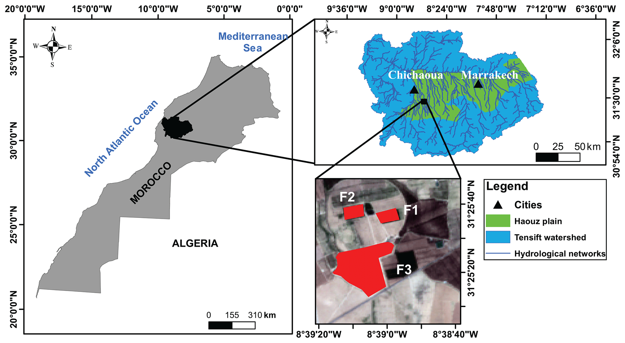
Figure 1 Location of the study fields: F1, F2 and F3 are drip-irrigated wheat plots in a private farm (Domaine Rafi) near the city of Chichaoua in the Haouz plain, central Morocco.

2.2 Experimental sites

The database concerns three irrigated fields (F1, F2 and F3) located within a private farm in the province of Chichaoua located 65 km west of Marrakech city (Fig. 1). F1 and F2 are monitored during two successive growing seasons (2016/17 and 2017/18), while F3 is monitored during the season 2018/19. The fields are sown using an automatic seed drill. They are irrigated using the drip technique. For all the fields, the wheat is cropped once a year during winter–spring (see Table 1 for sowing and harvest dates). After harvest, the fields are generally used for cattle grazing until mid-July when the plowing work starts. Table 1 summarizes some general information about the fields. Please note that during the 2017/18 season, wheat in F2 was affected by specific growing conditions: (i) the development of adventices belonging to the wild thistle family characterized by a horizontal structure, (ii) the seeding density being higher than in F1, and (iii) the seeding being a mixture of barley and wheat within F2. This resulted in very long stems: 146 cm in F2 compared to 110 cm in F1 in April 2018. Finally, these long stems in F2 were laid down by the wind from 12 April 2018. A picture of F2 during 2017/18 is provided in Appendix A (Fig. A1). Although such exceptional growing conditions are not very likely, it has been chosen to include this crop season in the data set to cover different conditions of growth.

Table 1 General information about the three fields.

3 Database

3.1 Field data sets

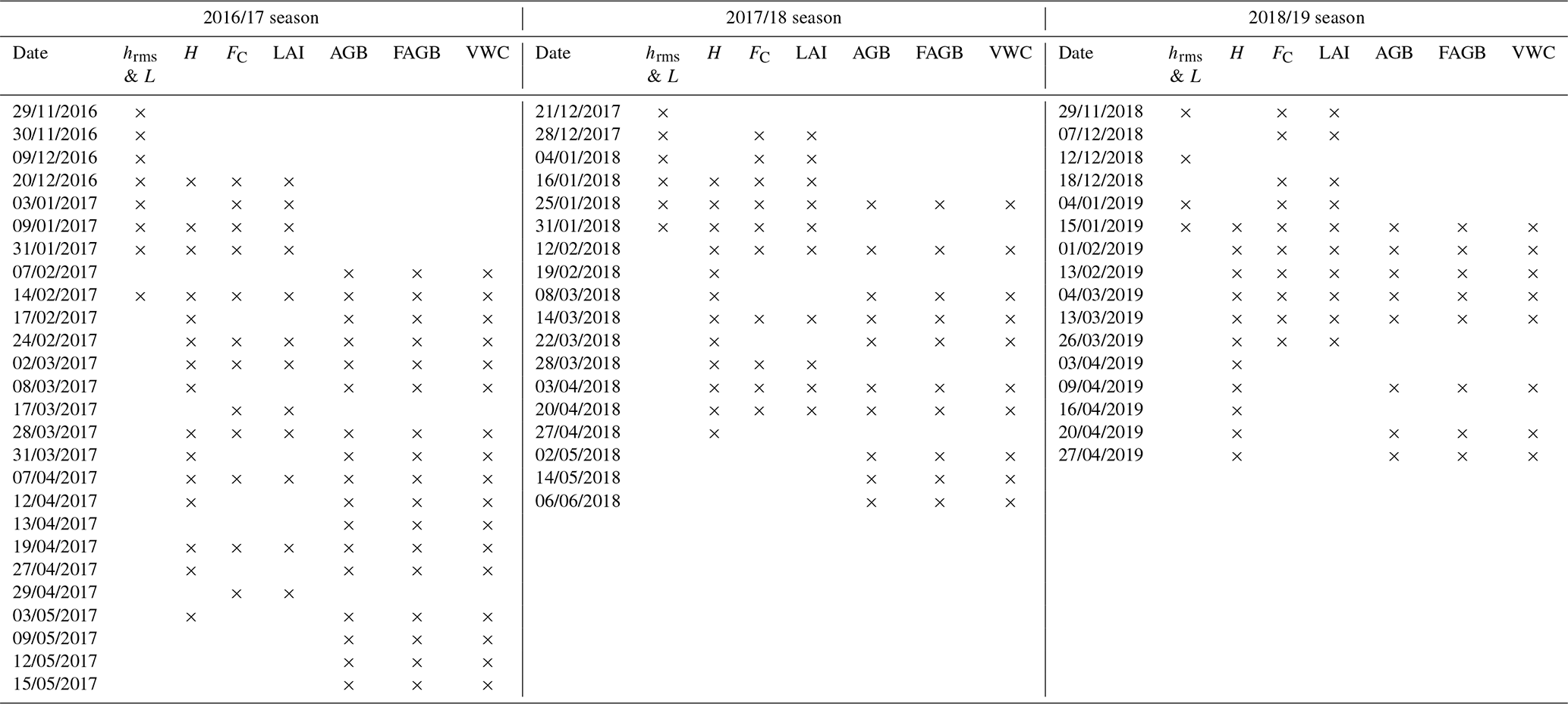
The field data sets consist of automatic measurements of soil moisture and weather data in addition to field surveys for surface roughness, biomass, vegetation water content, canopy height, the green leaf area index and the cover fraction. Table A1 in the Appendix summarizes the details of the 26, 18 and 16 field campaigns carried out during the 2016/17, 2017/18 and 2018/19 seasons, respectively.

3.1.1 Soil moisture

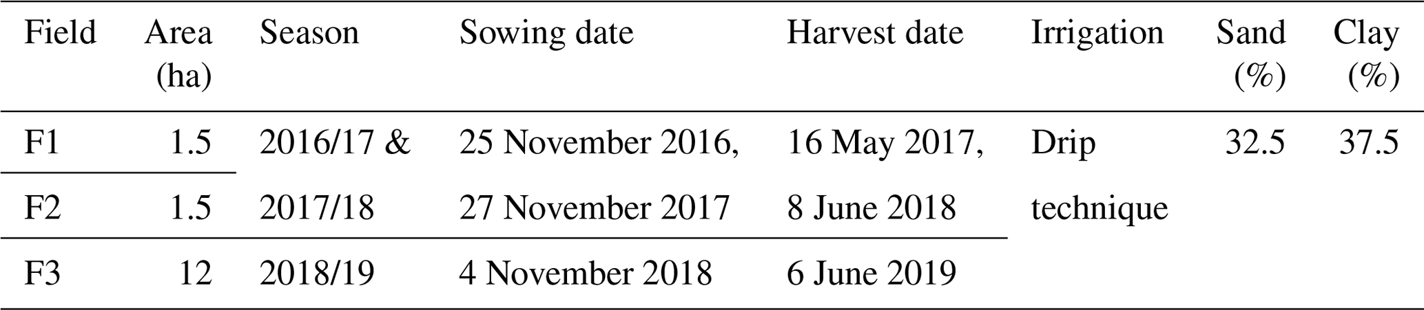
SSM is automatically measured every 30 min using time domain reflectometry (TDR) sensors (Campbell Scientific CS616) using two sensors buried at a depth of 5 cm: one under the drippers and another one between them. The average is computed in order to obtain a representative SSM value of the field. In addition, similar sensors are buried for RZSM measuring at 25 and 35 cm of depth in F1 and F3, while one sensor is buried at 30 cm in F2 because of the lack of an additional sensor. Figure 2a illustrates an example of TDR sensors at different depths.

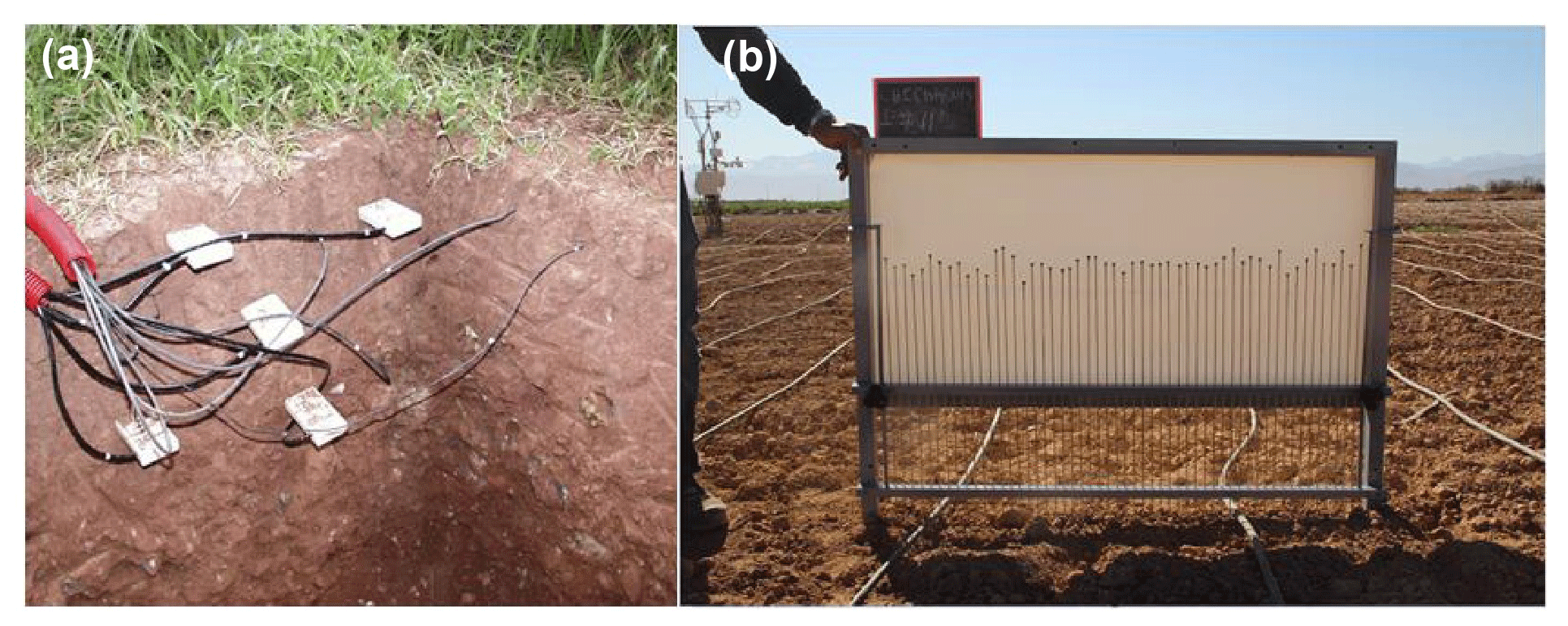
Figure 2 Examples of (a) TDR sensors installed at different depths and (b) a pin profiler picture taken over one of the plowed field with drip irrigation tubes installed.

TDR sensors are calibrated using the gravimetric technique. The calibration is performed during the 2016/17 season using samples taken from the first 5 cm from both fields F1 and F2, and then the calibrated equation is applied to F1, F2 and F3 data as the soil characteristics are similar and the same sensors are used. For that purpose, an aluminum core of 392.5 cm³ is used to collect samples at the TDR installation depths. Three samples are collected per day and per field during 5 d chosen with different soil moisture conditions in order to cover a wide range of values (0.08 to 0.33 m³ m⁻³). A linear regression is established between the volumetric water content and the square root of the TDR time response (named τ, in seconds) as follows:

$$\begin{array}{}\text{(1)}& \mathrm{SSM}=a_{\mathrm{TDR}}\times \sqrt{\mathit{\tau }}+b_{\mathrm{TDR}}.\end{array}$$

The calibrated values using data of both fields are a_TDR=0.275 m³ m⁻³ s^−0.5 and $b_{\mathrm{TDR}}=-\mathrm{1.154}$ m³ m⁻³. Figure 3 illustrates the calibration results with all the samples displayed. The statistical metrics are the correlation coefficient R = 0.97, root mean square error RMSE = 0.018 m³ m⁻³ and no bias. When considering both fields separately, the results for (F1, F2) are R = (0.90, 0.94), RMSE = (0.023, 0.01) m³ m⁻³ and bias = (−0.002, 0.003) m³ m⁻³.

Figure 3 Surface soil moisture measured by TDR versus gravimetric measurements using samples collected in both fields F1 and F2 during the 2016/17 growing season. The solid blue line is the linear regression, and the dashed line is Y=X.

The calibrated equation is also applied for the RZSMs assuming that the soil properties are the same at different depths. Figure A2 in Appendix A illustrates an example of an RZSM time series in F1.

3.1.2 Surface roughness

Surface roughness characterizes the micro-variation in the ground surface elevation within a given area/field (Allmaras et al., 1966). It affects particularly the SAR signal and to a lesser extent the visible and near infrared (Girard and Girard, 1989). The two parameters that characterize the surface roughness are the root mean square height (h_rms) and the correlation length (L). h_rms provides a vertical descriptor of ground roughness by measuring the elevation of the surface along one or more observation lines and calculating the standard deviation of the recorded values. The second parameter (L) corresponds to the distance between measurements from which the heights between points are statistically independent. This parameter provides a horizontal description of the ground surface roughness, more specifically the organizational structure and spatial continuity of the microtopography (Nolin et al., 2005). Over the three studied fields, measurements of the surface roughness are taken during the first stage of wheat (from emergence to early tillering) when the ground is not totally covered by the canopy. We used a pin profiler of 1 m length, composed of a set of 53 metal needles of equal length every 2 cm (Fig. 2b). A total of 16 sample pictures are taken per field and per date including 8 pictures parallel and 8 pictures perpendicular to the rows' direction. The pictures are taken using a Canon 6EOS 600D equipped with a Tamron lens (Model A14).

Table 2 Average values of the roughness parameters (eight samples are gathered per field and per direction).

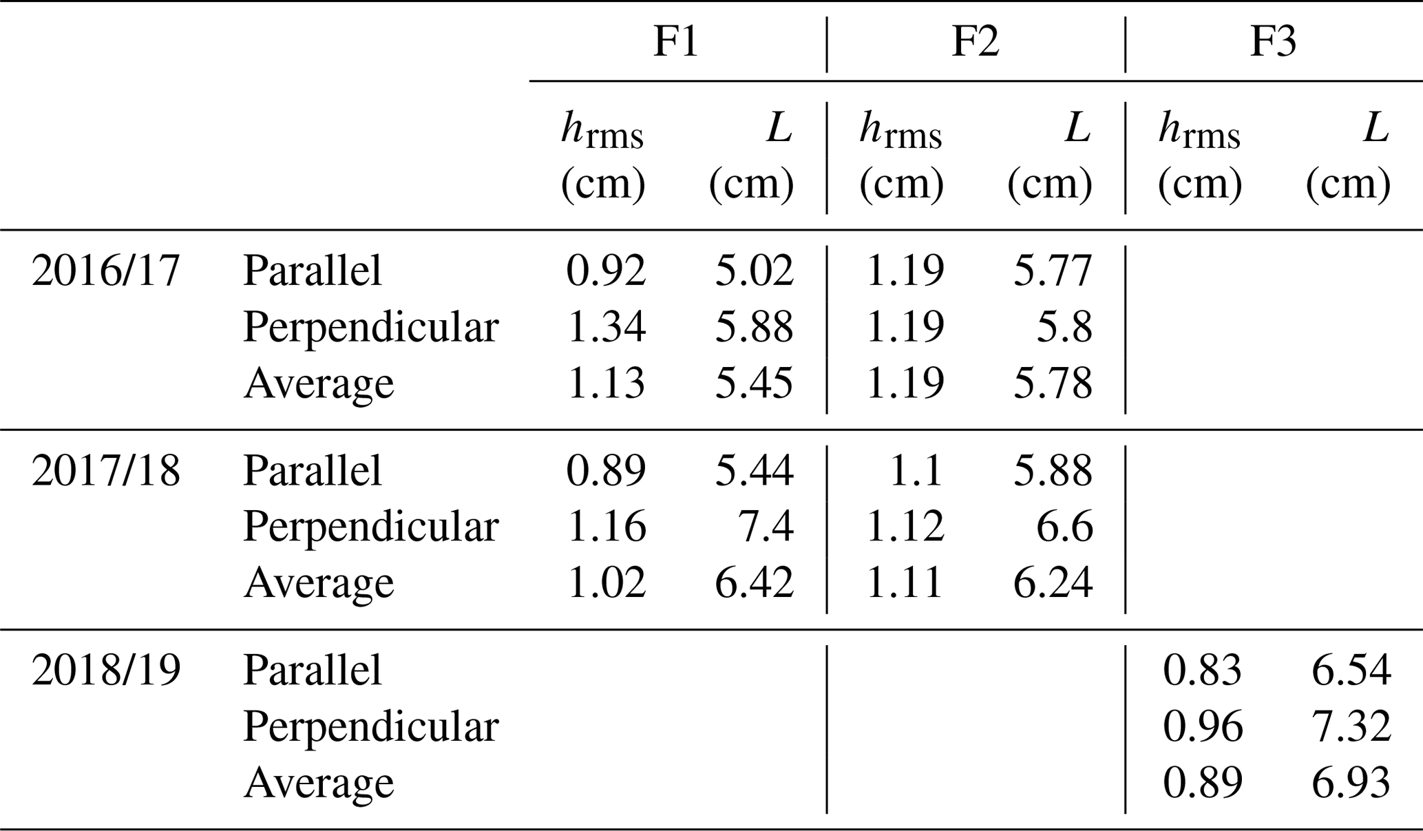
The images are processed in MATLAB based on the detection of the top position of each needle. h_rms and L are computed from the auto-correlation function, and then the average per direction, per field and per date is computed. For illustration, Fig. 4 shows the time series of h_rms and L parameters computed separately for each direction for F1 and F2 during the season 2017/18, while the average values per season are summarized in Table 2 for F1, F2 and F3.

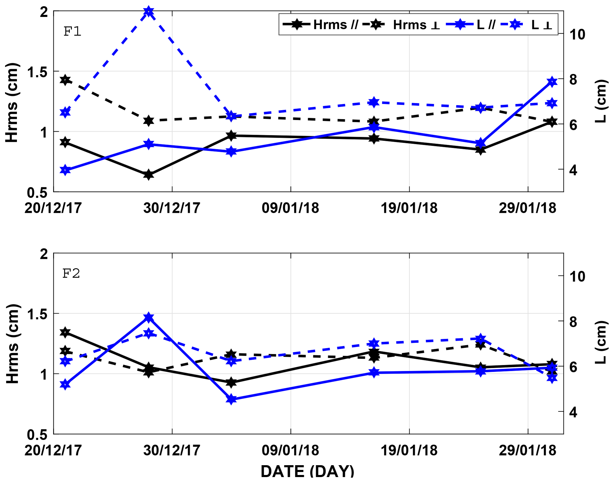
Figure 4 Time series of h_rms and L computed from parallel and perpendicular measurements separately for F1 and F2 during the season 2017/18.

Based on the range of h_rms measurements (0.83 < h_rms < 1.35), it can be clearly seen that the fields are characterized by a slightly rough or smooth surface, which is generally the case for disc-tilled fields. After sowing, a slight change is observed at the start of the crop season (28 December 2017; see Fig. 4). At that time, the soil has just been prepared for sowing and rows are directly exposed to rain. The fact that the rows are still visible in the field also explains the differences observed between both directions early in the season. This anisotropy disappeared quickly with irrigation, rainfall and plant growth. h_rms and L are almost constant from early January onwards. Indeed, it has been shown that after sowing, roughness is affected by very limited temporal variations (Bousbih et al., 2017) as no soil works occur after sowing. It is usually kept constant during the crop season (El Hajj et al., 2016; Gherboudj et al., 2011; Gorrab et al., 2015; Ouaadi et al., 2020b).

3.1.3 Biomass and water content

Biomass and water content are two biophysical parameters of crucial importance in different agricultural applications including particularly plant stress monitoring, radar backscattering response, crop yield and evapotranspiration modeling. Within each field, eight samples are collected once a week/every 2 weeks during the growing season. The samples are chosen randomly so that the average is representative of the plot. A quadrate of an area of 0.0625 m² is used for the sampling (Fig. 5). The samples are weighed first in the field to obtain fresh aboveground biomass (FAGB). The corresponding aboveground biomass (AGB) expressed in kilograms of dry matter per square meter is determined at the laboratory by drying the samples in an electric oven at 105 ^∘C for 48 h. The vegetation water content (VWC) is thus computed as the difference between FAGB and AGB (Gherboudj et al., 2011).

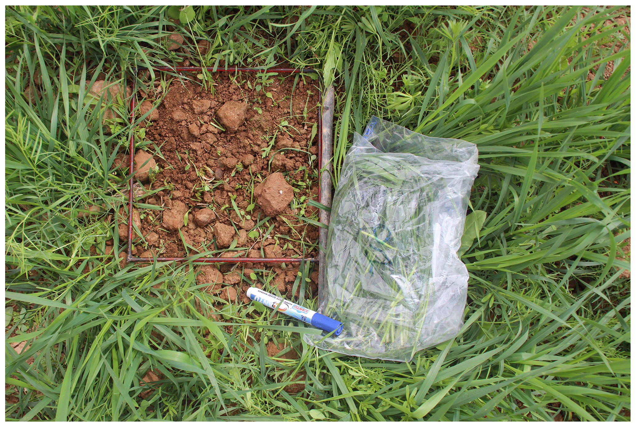
Figure 5 Photo taken during a measurement campaign illustrating a sample of aboveground biomass measurement.

3.1.4 Canopy height, green leaf area index and cover fraction

The canopy height (H), green leaf area index (GLAI) and cover fraction (F_C) are measured every week during the growing season. Values from 11 different places are averaged and considered a representative measure of the field. H is simply measured using a measuring tape, while the GLAI and F_C are computed by processing hemispherical photos (Fig. 6b) using MATLAB software following the method described in Duchemin et al. (2006) and Khabba et al. (2009). The eight photos per date and per field are taken using a Canon 6EOS 600D camera with a SIGMA 4.5 mm F2.8 EX DC circular fisheye HSM (Fig. 6a). Photos are taken in optimal lighting conditions to avoid shadow effects and over-exposure phenomena which make classification more difficult. The algorithm is based on the binarization of the hemispherical images by thresholding a greenness index. Next, the useful part of the images is extracted by masking the operator and the high viewing angles (> 75^∘) (Fig. 6c). Finally, the ground-covered area is extracted on concentric rings associated with fixed viewing angles, and the average of all pictures is the field GLAI. Using the same process, F_C is calculated as the ratio of the vegetation pixel number to the total pixel number.

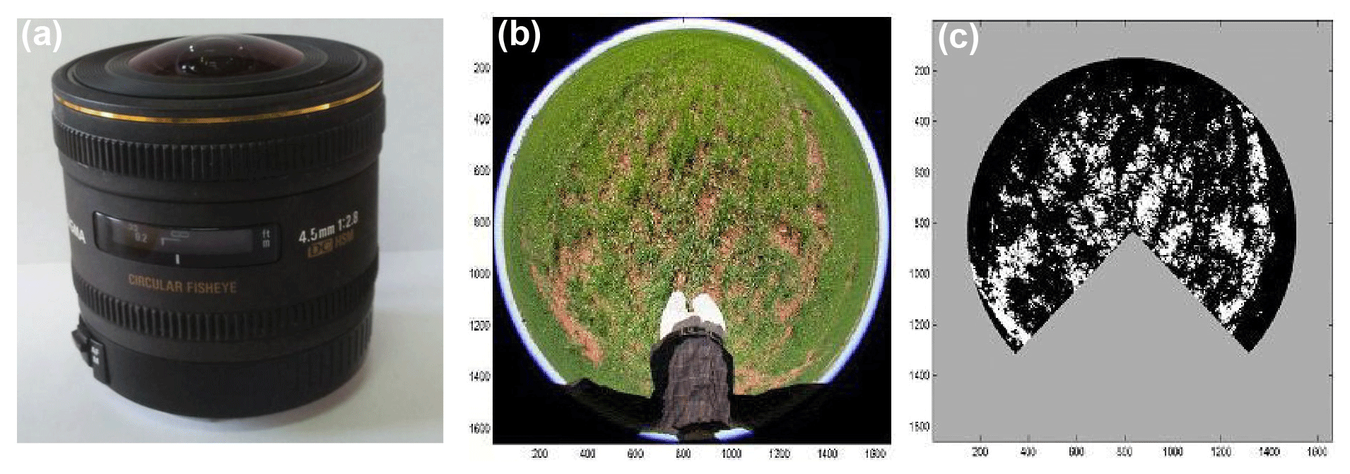
Figure 6 (a) The 4.5 mm F2.8 EX DC circular fisheye HSM, (b) a hemispherical photo, and (c) the result of the processing after binarization and after masking the operator and the high viewing angles (> 75^∘).

3.1.5 Irrigation and weather data

F1, F2 and F3 are irrigated using the drip technique. Irrigation quantities are determined by the farmer by estimating the daily evapotranspiration under standard conditions (ET_c) in the region computed using the FAO 56 model simple approach (Allen et al., 1998). The cumulative ET_c for a given period (usually 1 week) is applied during one or more events per week depending on the farmer's constraints (e.g., availability of workforce) and on the weather conditions (e.g., occurrence of rain). The irrigation pipes are spaced by 0.7 m, while the distance between the drippers along the pipe is 0.4 m. In F1 and F2, the flow rate of each dripper is 7.14 mm h⁻¹. The irrigation takes place for about 105 min (12.53 mm). A flowmeter mounted downstream of a valve allowed an accurate collection of irrigation volumes. F2 and F3 are irrigated according to FAO recommendations, while F1 is stressed voluntarily. The stress involved in F1 is during the first season (2016/17) only. By contrast, the 2017/18 season was wet, so there is no clear stress observed on the field. The irrigation dates and amounts in F1 and F2 during both seasons are made available throughout this database, while the irrigation in F3 is not available.

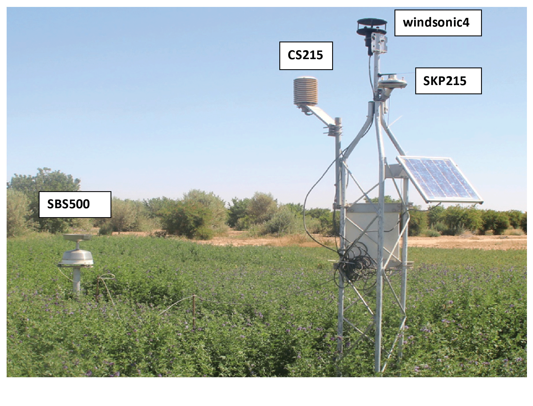
The weather data including precipitation, air temperature, relative humidity, solar radiation, and wind speed and direction are collected by an automatic weather station installed over an alfalfa field near the studied fields (Fig. 7). The weather station provides continuously meteorological data every 30 min. The Campbell sensor CS215 is used to measure the air temperature and the relative humidity (Fig. 7). The global solar radiation and the wind direction and speed are measured using the Campbell SKP215 and Campbell WindSonic4, respectively. The precipitation is measured using the rain gauge (Campbell SBS500) shown in Fig. 7.

Figure 7 Automatic weather station installed in an alfalfa field near F1, F2 and F3.

3.2 Remote sensing data sets

3.2.1 Sentinel-1

Sentinel-1A (S1A) and Sentinel-1B (S1B) are Earth observation satellites developed for the Copernicus initiative and launched by the European Space Agency in April 2014 and April 2016, respectively. During full operation, S1A and S1B are maintained in the near-polar Sun-synchronous orbit at 693 km in altitude, phased 180^∘, providing a revisit time of 6 d (Torres et al., 2012). Sentinel-1 (S1) is a synthetic aperture radar operating at the C-band with a frequency of 5.33 GHz, mapping the entire world in 175 orbits per cycle. The main operational imaging mode is the Interferometric Wide (IW) swath mode. IW acquires data with a wide swath of 250 km with high geometric (azimuth resolution 20 m and ground range resolution 5 m) and radiometric resolution (European Space Agency, 2012). The IW mode supports operation in single and dual polarization (HH, VV, HH–HV and VV–VH) and covers a range of incidence angles between 31 and 46^∘. The product is composed of three sub-swaths acquired with the TOPSAR imaging technique which significantly reduces the scalloping effect (De Zan and Guarnieri, 2006).

Level-1 products are systematically processed and available within 24 h, free of charge from the Copernicus Open Access Hub website (https://scihub.copernicus.eu, last access: 19 July 2021). The website provides data for two types of products: GRDH (Ground Range Detected High Resolution) and SLC (Single Look Complex).

Table 3 Characteristics of the sentinel-1 products processed over the three fields for the monitored periods.​​​​​​​

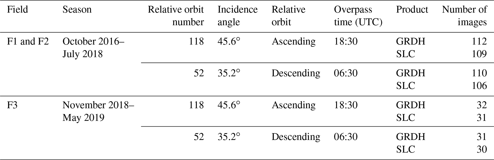
In this database, 561 GRDH and SLC products are processed (Table 3). Among them, 124 images are acquired over F3 during the 2018/19 growing season and 437 over F1 and F2 from 1 October 2016 to 31 July 2018, along the ascending no. 118 (221 images) and descending no. 52 (216 images) relative orbits. This period includes two agricultural seasons in addition to the summer period.

Backscattering coefficient

GRDH products are provided by ESA with a square pixel size and contain only the intensity information. The backscattering coefficients are extracted using the Orfeo ToolBox (CNES, 2018). The processing procedure consists of three steps (Frison and Lardeux, 2018):

1. Thermal noise removal. The SAR product contains not only the useful signal but also the unwanted noise disturbing the information contained in the intensity images, especially when the backscattered power is low. The thermal noise is an additive noise. The compensation for this noise can be performed by subtracting the scaled noise power using the calibrated noise vectors provided by ESA.

2. Calibration. The calibration step aims to convert the digital accounts into a physically interpreted parameter: the backscattering coefficient. A calibration vector included in the GRDH products contains the necessary information to convert the digital values to the backscattering coefficient.

3. Terrain correction. S1 SAR data are sensed with a viewing angle greater than zero which induces distortion in the products because of the lateral viewing geometry. The “Terrain correction” module is used to compensate for these distortions and obtain as many images as possible with real geometric representation. The images are projected on the Earth's surface using a digital elevation model (DEM). The SRTM (Shuttle Radar Topography Mission) DEM of 30 m resolution is used according to the method described in Small and Schubert (2008).

SAR images are affected by the speckle noise, which is mainly due to the relative phase of individual scatters within a resolution cell. Many filters have been developed to remove the speckle noise although the best filter is the spatial average. The presented database is generated using a simple average per field of 120, 121 and 1100 pixels for F1, F2 and F3, respectively, with a mean standard deviation of around 1.55 dB. In order to visualize data dynamics, backscattering coefficients are converted into decibels.

Interferometric coherence

Sentinel-1 SLC products are provided in slant-range geometry. They contain three sub-swath images: IW1, IW2 and IW3. Each sub-swath is composed of nine bursts with black-fill demarcation. By contrast with GRDH, both intensity information and phase information are kept. The phase information is used for the computation of interferometric coherence. SAR interferometry consists of correlating two images acquired from two positions in space slightly separated from each other (with two radars mounted on the same platform) or at different times by exploiting repeated orbits of the same satellite such as for Sentinel-1. Thanks to its high temporal resolution (6 d per orbit), the interferometric coherence is computed from two consecutive acquisitions of the same orbit.

The interferometric coherence, given by Eq. (2), for a local neighborhood of N pixels, is generated by cross-multiplying, pixel by pixel, the first SAR image z_i with the complex conjugate ${z_i^{\prime }}^{\ast }$of the second (Bamler and Hartl, 1998; Touzi et al., 1999).

$$\begin{array}{}\text{(2)}& \mathit{\rho }={\displaystyle \frac{\sum _{i=\mathrm{1}}^N{z}_i\cdot {z_i^{\prime }}^{\ast }}{\sqrt{\sum _{i=\mathrm{1}}^N{\left|z_i\right|}^{\mathrm{2}}\cdot \sum _{i=\mathrm{1}}^N{\left|z_i^{\prime }\right|}^{\mathrm{2}}}}}\end{array}$$

The interferometric coherence $\left|\mathit{\rho }\right|$ varies between zero (incoherence) and 1 (perfect coherence). The interferometric coherence is related to the movements of the scatterers within a given canopy. It decreases (loss of coherence) in the case of dense vegetation, while high values are obtained over bare soils. Loss of coherence could be caused by the temporal interval between acquisitions, orbit errors, vegetation development/movement or processing errors. The random dislocation of scatters because of the weather (wind and rain) or the plants' growth is the main cause of the temporal decorrelation.

The Sentinel application platform SNAP is used to compute the interferometric coherence from S1 SLC products in five steps (Veci, 2015):

1. Apply-Orbit-File. This module is applied for a better estimation of the position and speed of the satellite using the orbit state vector. Preliminarily, a predicted orbit state vector is contained in the metadata, but it is not accurate. The precise orbit is made available 1 month after data acquisition at the latest. For this reason, the automatic download in SNAP is used in order to update the orbit state vectors.

2. Back-Geocoding. The two images need to be co-registered. One of the images is the master, and the other is the slave. This step ensures that each pixel of the slave image is aligned with the corresponding pixel in the master image so that both pixels contain contributions from the same target. The DEM is required for the Back-Geocoding step; SNAP allows us either to enter it manually or to download it automatically.

3. Coherence. This module in SNAP allows the computation of the interferometric coherence between the two images for a given local neighborhood. In order to obtain a square pixel of 13.95 m, azimuth × range is fixed to 3 × 15 in the processing.

4. TOPSAR-Deburst. The black fills in between bursts are deleted separately for both polarization images (VV and VH).

5. Terrain-Correction. Finally, the processed images are projected on the Earth's surface using a DEM.

3.2.2 Sentinel-2 NDVI

Sentinel-2 optical satellites S2A and S2B were launched by ESA in June 2015 and March 2017, respectively. They are placed in opposition on the same orbit at an altitude of 800 km. Sentinel-2 provides data every 5 d with a width of 290 km and a resolution of 10 to 60 m according to spectral bands (13 bands) ranging from visible to the medium infrared. The National Centre for Space Studies (CNES) provides Level-2A products atmospherically corrected free of charge via PEPS (https://peps.cnes.fr/, last access: 19 July 2021) or the Theia website (https://theia.cnes.fr/, last access: 19 July 2021). Data are corrected for atmospheric effects by the Center for the Study of the Biosphere from Space (CESBIO) using the MAJA chain (Hagolle et al., 2015). The atmospheric corrections are performed in three steps:

1. The satellite top-of-atmosphere (TOA) reflectances are corrected for the absorption by the atmospheric gas molecules using the absorption part of the Simplified Model for Atmospheric Correction (SMAC) method by Rahman et al. (1994). The concentrations of the ozone, the oxygen and the water vapor are obtained from satellite data (ozone) and meteorological data (water vapor, pressure).

2. The detection of the clouds (and clouds' shadows) is based on the multi-temporal cloud detection method proposed by Hagolle et al. (2010).

3. The estimation of the aerosol optical thickness (AOT) relies on a hybrid method merging the criteria of a multi-spectral method with the multi-temporal technique developed initially for the VENµS satellite mission by Hagolle et al. (2010). The AOT is used along with the surface altitude, the viewing geometry and the wavelength in the parameterization of look-up tables for the conversion of TOA reflectances already corrected in step 1 into surface reflectances. The look-up tables are provided by the successive orders of scattering code (Lenobel et al., 2007) used in the modeling of molecular and aerosol scattering effects. A different look-up table is computed for each aerosol model.

Data are downloaded from the Theia site. Among the available products, only the products non-covered with clouds are used corresponding to 10, 25 and 26 images for the 2016/17, 2017/18 and 2018/19 agricultural seasons, respectively. Please note that during the season 2016/17, only S2A was in the orbit which explains the limited number of images (10). Next, the normalized difference vegetation index (NDVI) corresponding to each pixel is computed from band 4 and 8. An average per field is used to compute the time series of each field.

4 Data analysis

4.1 Vegetation variables

In this section, the relationships between the different variables (GLAI, FAGB, AGB, VWC and H) that characterize the vegetation growth and development are first investigated. These relationships are extensively used for different applications such as the calibration of backscattering models and the development of retrieval approaches (Chauhan et al., 2018). Several land surface or crop models rely on empirical relationships to predict F_C or H as well (Bigeard et al., 2017; Castelli et al., 2018). Other agricultural models compute AGB from the GLAI using linear or polynomial relationships (Major et al., 1986; Petcu et al., 2003). Figure 8 displays the resulting relationships using data from F1 by selecting only the 2016/17 season for illustrative purposes. These relationships are computed separately based on the data recorded before and after the peaks of the GLAI and FAGB.

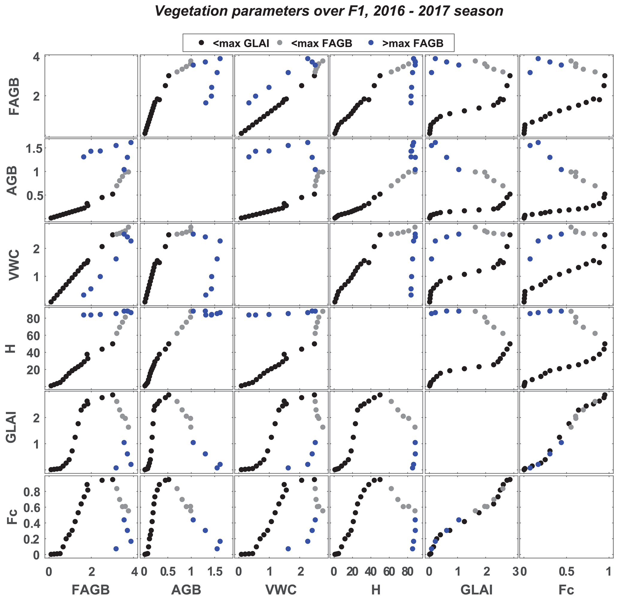
Figure 8 Scatterplots of the relationships between wheat measured variables: FAGB, AGB, VWC, H, GLAI and F_C. Data are presented separately using the maximum of the GLAI and FAGB as thresholds: data < max GLAI are in black; data < max FAGB (and > max GLAI) are in grey, and data > max FAGB (and > max GLAI) are in blue.

The nature of the relationship changes depending on the structure (biomass variables) or on the greenness of the plant (GLAI). The biomass variables (FAGB, AGB and VWC) and H increase up to the biomass peak. Afterwards, a reverse evolution can be observed, characterized in particular by a decorrelation between FAGB/VWC and AGB. This is mainly related to the senescence process of the vegetation; the leaves begin to dry progressively with the start of the grain filling, so the sap flow (water, carbohydrates, proteins and mineral salts) migrates to the heads at the top of the plant (Farineau and Morot-Gaudry, 2018). Indeed, VWC and AGB are highly correlated until the vegetation peak (the correlation coefficient is R = 0.94 before the peak and R = −0.20 afterwards), while FAGB being dominated by the plant water content is highly correlated with VWC during the whole crop season (R = 0.99 before the peak, and R = 0.98 afterwards). Likewise, H is highly correlated to FAGB, VWC and AGB until the vegetation peak (R > 0.97) when H remains at its maximum value while AGB continues to increase with grain filling and VWC and FAGB decrease because of the vegetation drying. The relationship of these variables (FAGB, AGB, VWC and H) with the GLAI and F_C is quite different. The curves are of a parabolic shape with a maximum reached around the GLAI peak. A timing shift between the peaks of the GLAI and FAGB is observed. This is probably related to the senescence of the lower leaves, which leads to an earlier drop of the GLAI than of FAGB. Between the peaks of the GLAI and FAGB, the GLAI decreases while (i) AGB and H increase and (ii) FAGB increases slightly while VWC is almost constant. After the FAGB peak, AGB goes on increasing due to grain filling while the VWC decreases due to drying of the plant. FAGB, which is the sum of AGB and VWC, is almost constant.

4.2 Radar data

The time series of the backscattering coefficient, the polarization ratio and the interferometric coherence are analyzed here for two agricultural seasons and a summer period on F1 and F2 and at two incidence angles (35.2 and 45.6^∘).

4.2.1 The backscattering coefficient

Figure 9 displays the time series at 45.6^∘ in F2 for illustrative purposes: (a) backscattering coefficient at VV polarization (${\mathit{\sigma }}_{\mathrm{VV}}^{\mathrm{0}}$); (b) backscattering coefficient at VH polarization (${\mathit{\sigma }}_{\mathrm{VH}}^{\mathrm{0}}$) as well as wheat phenological stages; (c) SSM, air temperature, irrigation and rainfall. Figures A3–A5 in Appendix A show the same time series in F1 and F2 at 35.2^∘ and F1 at 45.6^∘, respectively. The backscattering coefficients reveal a strong seasonal signal with two cycles. The first cycle takes place from sowing to the heading stage, and the second takes place from heading to harvest with the minimum reached around the heading stage. The highest values at 35.2^∘ are observed in the first cycle, while at 45.6^∘, σ^∘ is higher during the second peak. The maximum values of ${\mathit{\sigma }}_{\mathrm{VV}}^{\mathrm{0}}$ reached the same value for F1 and F2, while higher values are observed on F2 at VH. ${\mathit{\sigma }}_{\mathrm{VV}}^{\mathrm{0}}$ is more sensitive to soil moisture variation until mid-January, corresponding to the tillering stage, when the soil is not yet fully covered by vegetation. Although it is agreed that the signal during this period is governed by the dynamics of soil moisture, its behavior differs from one site to another, giving the difference in soil hydric conditions and surface roughness. After this period, the signal behavior is similar to the profiles obtained by Cookmartin et al. (2000), El Hajj et al. (2019), Nasrallah et al. (2019) and Veloso et al. (2017). It decreases gradually from the early tillering until the heading stage (around 13 March) by about 10 dB on F2 and 5 dB on F1 because of the attenuation by the canopy during the development of the stems (extension stage) (Cookmartin et al., 2000; Mattia et al., 2003; Picard et al., 2003; Wang et al., 2018). Obviously, the attenuation is more important at VV polarization because of the vertical structure of wheat (stems) in line with the results of Fontanelli et al. (2013), Picard et al. (2003) and Wang et al. (2018). The response of ${\mathit{\sigma }}_{\mathrm{VH}}^{\mathrm{0}}$ to SSM variation and canopy attenuation is lower than for ${\mathit{\sigma }}_{\mathrm{VV}}^{\mathrm{0}}$. After the heading stage, the signal starts to increase again. This is clearer on F2 than on F1 and at 45.6^∘ than at 35.2^∘. The heading stage is the phenological stage of wheat when the spike or head starts emerging out from the leaf sheath. This change in the structure of the canopy shields the stems from the radar signal through the appearance of a thick, wet, top layer composed of the heads. The C-band wavelength penetrates this layer only, resulting in increased volume scattering, while attenuation becomes low. This effect is stronger for F2 than for F1, at VH than at VV and at 45.6^∘ than at 35.2^∘. This increase was first reported by Ulaby and Batlivala (1976). Subsequently, Ulaby et al. (1986) suggested that an additional term must be added to the traditional three-term model (vegetation volume diffusion, soil attenuation and soil–vegetation interaction) to properly represent wheat backscattering after heading. Later on, similar behavior was observed and attributed by numerous authors to the appearance of the heads followed by the grain (Brown et al., 2003; El Hajj et al., 2019; Mattia et al., 2003; Patel et al., 2006; Veloso et al., 2017). The exceptional growing conditions in F2 during the 2017/18 season is behind the origin of the observed plateau of the backscattering coefficient which remains quite stable until harvest. This is due to a significant contribution of volume scattering which is a behavior that characterizes a crop developing a random canopy structure in relation to the numerous and dense adventices as already highlighted (see picture Fig. A1 in Appendix A).

Figure 9 Time series of the backscattering coefficient at VV (a) and VH (b) polarizations on F2 at a 45.6^∘ incidence angle during the period from 1 October 2016 to 31 July 2018. The tilling works and phenological stages of wheat are superimposed in panels (a) and (b), respectively. The air temperature, surface soil moisture (SSM), irrigation and rainfall are displayed in panel (c).

The low variation observed on F1 during the 2016/17 season is mainly related to the limited development of vegetation because of the triggered water stress. Likewise, the difference between the two seasons in F2 is related to a higher density of grown seeds and wetter conditions in the 2017/18 season compared to 2016/17 (the amount of rainfall during the growing season – from sowing to harvest – reached 167.23 mm in 2017/18 while only 69.94 mm is recorded in 2016/17). With the drying of the head layer, the backscattering decreases again at the end of the season to reach the lower observed values. Indeed, as the head layer dries, the vegetation becomes transparent to the signal. The soil is also dry at the end of the season because irrigation is stopped. These low values remain until the first deep plowing on 11 July, when a sharp increase is observed because of a drastic change in soil roughness. Hereafter, the signal is again stable until the seedling preparation work for the next 2017/18 season (22 November).

4.2.2 The interferometric coherence and the polarization ratio

Figure 10 displays the time series at 45.6^∘ in F2 of the (a) interferometric coherence at VV (ρ_VV) and VH (ρ_VH) polarizations together with sowing and tilling dates; (b) polarization ratio (PR = ${\mathit{\sigma }}_{\mathrm{VH}}^{\mathrm{0}}/{\mathit{\sigma }}_{\mathrm{VV}}^{\mathrm{0}}$), as well as wheat phenological stages; (c) Sentinel-2 NDVI and measured GLAI; and (d) measured FAGB, AGB, VWC and H. Likewise, Figs. A6–A8 in Appendix A display the time series in F1 and F2 at 35.2^∘ and F1 at 45.6^∘, respectively. The time series of ρ_VV and ρ_VH follows a similar evolution. Before sowing, coherence is at its highest value corresponding to 0.9 for ρ_VV and 0.7 for ρ_VH (Fig. 10a). These values express a dominance of coherent scattering, corresponding to the response of bare soils composed of big rocks. Indeed, during the summer, the plots are subjected to deep plowing which yields big clods that resist any change in surface structure caused by climatic factors such as wind or rain. The second tilling breaks up the clods for the next seeding. Soil works and farming activities induce a large decrease in coherence in line with the observation of Wegmuller and Werner (1997). The surface roughness is a main parameter that influences not only the amplitude at the C-band but also the phase. Indeed, abrupt drops are observed around each sowing event and tilling works (vertical brown lines in Fig. 10a).

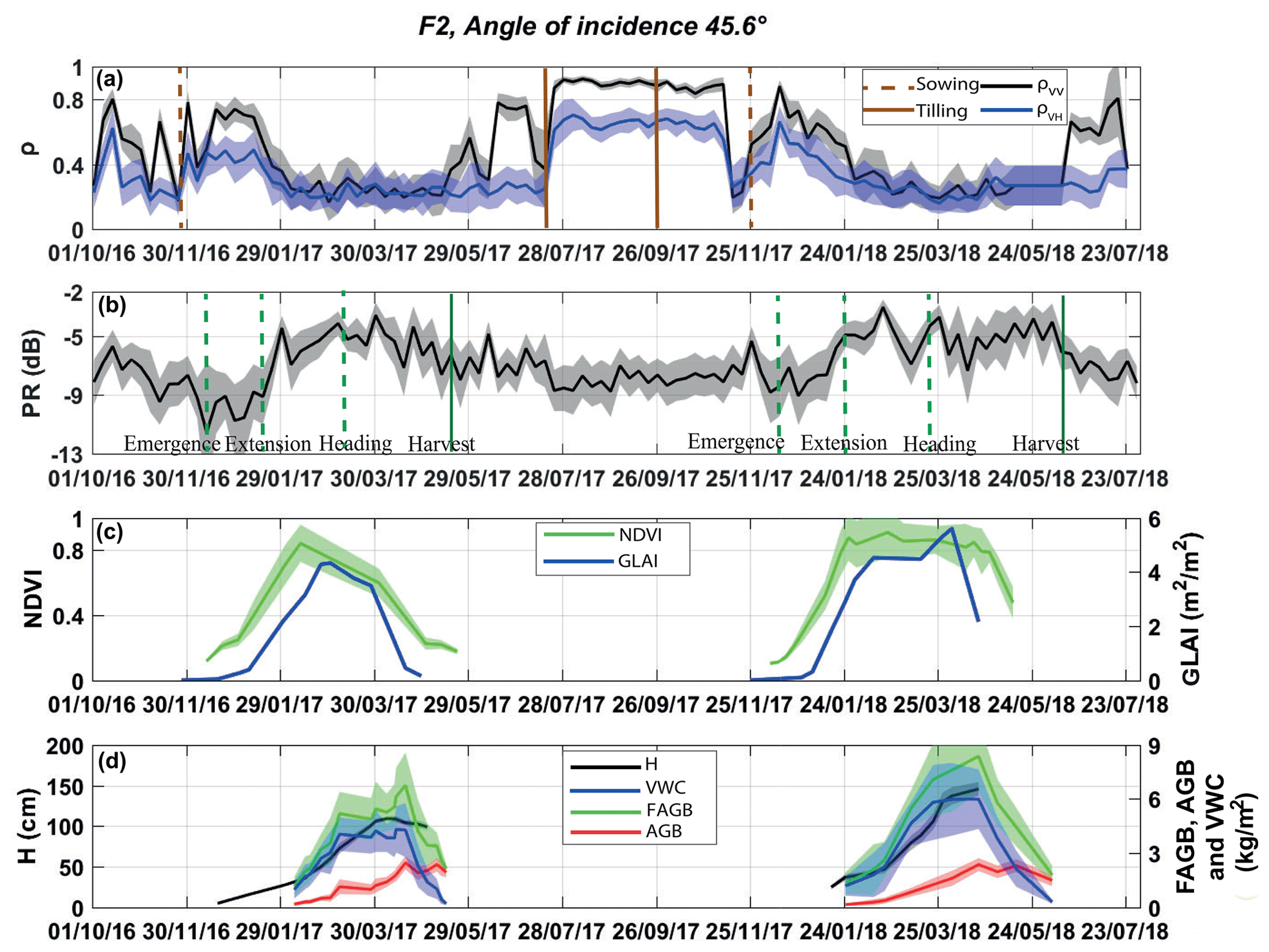
Figure 10 Time series of the interferometric coherence at VV and VH polarizations (a) and the polarization ratio (b) on F2 at a 45.6^∘ incidence angle during the period from 1 October 2016 to 31 July 2018. The tilling works and phenological stages of wheat are superimposed in panels (a) and (b), respectively. The NDVI and measured GLAI are displayed in panel (c). Measured H, FAGB, VWC and AGB are plotted in panel (d). Time series are presented by mean values (solid lines) and standard deviations (shading surrounding the solid lines).

After sowing, the evolution is similar to that of the profiles obtained by Blaes and Defourny (2003) and Engdahl et al. (2001). The interferometric coherence increases from 0.15 to 0.7 and then starts to decrease slightly from the emergence of wheat, becoming almost constant after stem extension with values < 0.3 corresponding to the noise level. Indeed, using the ERS-2–Envisat Tandem mission, Santoro et al. (2010) demonstrated that coherence measurements of vegetated fields are always below the level of bare soil coherence. Actually, the interferometric coherence is known to decrease exponentially with wheat growth (Lee et al., 2012). Vegetation growth and random dislocation of scatters cause a degradation of coherence (Blaes and Defourny, 2003; Engdahl et al., 2001; Wegmuller and Werner, 1997), especially under wind and rain effects. Between sowing and emergence, the observed variation is assumed to be related to the installation of irrigation drippers that took place up to 2 weeks after sowing. The changes that occur between the harvest and the first tilling could be attributed to livestock grazing, a common practice in the region after wheat harvest, which could change the surface roughness.

The polarization ratio (PR) is closely related to the biomass dynamic. Both increase from emergence to heading and then start to decrease until harvest. The maximum timing is around the middle of April. The significant differences in biophysical parameters between F1 and F2 are due to irrigation, as already highlighted for the backscattering coefficient time series. Likewise, the difference between the two seasons in F2 is related to a higher sowing density and wetter conditions in the 2017/18 season compared to 2016/17. As shown in Fig. 8, the time series of FAGB and VWC are in line with AGB and H up to the peak of FAGB and then decrease together while AGB continues to increase and H remains at its maximum value. FAGB and VWC drop at the same time but 50 d later when compared to the GLAI and NDVI and about 15 d before the backscattering coefficient.

4.3 Relationship between SAR data and vegetation variables

The polarization ratio and the interferometric coherence have been shown to be related to vegetation growth. In this section, the relationships between PR; ρ_VV and ρ_VH; and vegetation variables, including AGB, VWC, H, the GLAI and the NDVI, are analyzed. Figure 11 displays the results at a 35.2^∘ incidence angle, and Fig. A9 in Appendix A displays the results at 45.6^∘. H is used to illustrate the vegetation growth because its evolution is monotonic so that data corresponding to before and after maximum development can be easily separated. The determination coefficient R² and the Spearman rank correlation R_s are superimposed on the subplots together with the fitting equations using the whole database. Overall, a good correlation has been found between SAR variables (PR, ρ_VV and ρ_VH) and AGB, VWC, the GLAI and H. A hysteresis behavior is obviously observed for the vegetation variables with a non-monotonic dynamic (VWC, NDVI and GLAI). Using PR, the relationships are more scattered and characterized by lower saturation values. Although the range of variation of ρ_VH is limited with regards to PR, the statistical metrics of the relationships between interferometric coherences and the vegetation variables are better than those obtained using PR. ρ_VV exhibited better correlation with the vegetation variables than ρ_VH. With the exception of the NDVI, R_s is always greater than 0.67. The best fit is obtained between ρ_VV and H (R_s = 0.78, and R² = 0.65) with higher saturation values than the other relationships (∼ 55 % of H range which is about 77 cm). By contrast, a visual inspection of Fig. 11d, i and n shows that relationships with the NDVI are poorer when using data of the whole growing season. The dispersion is strong over the season. Data before and after the maximum development can be distinguished, particularly using ρ_VV and to a lesser extent ρ_VH. Figure 11i and n show that a linear relationship exists between the NDVI and SAR data using data before maximum development only, i.e., when the vegetation is still green. During the beginning of the season, the slope of ρ_VV–NDVI and ρ_VH–NDVI is low compared to the other vegetation variables. This is because the NDVI increases faster around the emergence of wheat while ρ_VV is still high because of the low vegetation cover fraction at this time. The hysteresis effect observed after the maximum of vegetation development is due to the senescence of the leaves when the NDVI starts decreasing while ρ_VV and ρ_VH are stable at low values.

Figure 11 Scatterplots of the relationships between PR; ρ_VV and ρ_VH; and AGB, VWC, H, the NDVI and the GLAI at a 35.2^∘ angle of incidence. The entire database from the three fields (F1, F2 and F3) is used. H is used to monitor the evolution during the growing season. All the determination coefficients (R²) and the Spearman rank correlations (R_s) are significant at 99 %.

When considering SAR data at a 45.6^∘ incidence angle (Fig. A9), a similar behavior to that shown in Fig. 11 is observed with AGB, VWC, H and the NDVI. The same hysteresis and scattering are observed for the NDVI although higher correlations are obtained. Similarly, ρ_VV is better correlated to vegetation variables than ρ_VH and PR. By contrast, the GLAI is better correlated with SAR variables than H. The PR–GLAI relationship is more scattered than at 35.2^∘ while the ρ_VV–GLAI relationship has the best metrics (R_s = 0.82, and R² = 0.73) with a higher saturation value around 50 % of the GLAI range (3 m² m⁻²).

Unlike PR, the metrics at both 35.2 and 45.6^∘ are stable for the relationships between ρ_VV and AGB, VWC and H. By contrast, the PR–GLAI relationship is more stable than the ρ_VV–GLAI relationship at both incidence angles.

4.4 Relationship between backscattering coefficient and SSM

Figure 12 displays the relationships between σ⁰ and SSM using the entire database at 45.6 and 35.2^∘ incidence angles. H is used as an indicator of vegetation growth. The correlation coefficient is computed separately for the entire database and for data corresponding to H lower than a threshold value (H_tr) corresponding to GLAI < 1.5. This value of the GLAI corresponds to wheat not fully covering the soil (Ouaadi et al., 2020b). H_tr is about 23.5, 23.5, 32.9 and 26 cm for F1 and F2 during 2017/18, for F2 during 2016/17 and for F3. Overall, ${\mathit{\sigma }}_{\mathrm{VV}}^{\mathrm{0}}$ is obviously better correlated to SSM than ${\mathit{\sigma }}_{\mathrm{VH}}^{\mathrm{0}}$, in line with the results of numerous studies (Holah et al., 2005; Li et al., 2014; Ulaby and Batlivala, 1976). Likewise, metrics at 35.2^∘ are better than those obtained at 45.6^∘. This is expected as the contribution of vegetation is dominant at higher incidence angles and at VH polarization. The relationships are scattered when using data from the whole season. This is attributed to the presence of vegetation and mainly to the attenuation of the soil signal backscattered by the wheat. The sensitivity of σ⁰ to SSM decreases progressively during the growing season as shown by the decreasing slope of the relationships with the vegetation development. By considering the early-season data only, when the soil is not yet covered by vegetation, a better fitting is obtained between σ⁰ and SSM. Indeed, the correlation coefficient using data with H < H_tr is improved whatever the polarization and the incidence angle. Obviously, the highest correlation is obtained at VV polarization and a 35.2^∘ incidence angle (R = 0.73) and to a lesser extent at VV at 45.6^∘ and VH at 35.2^∘ with R ≥ 0.66.

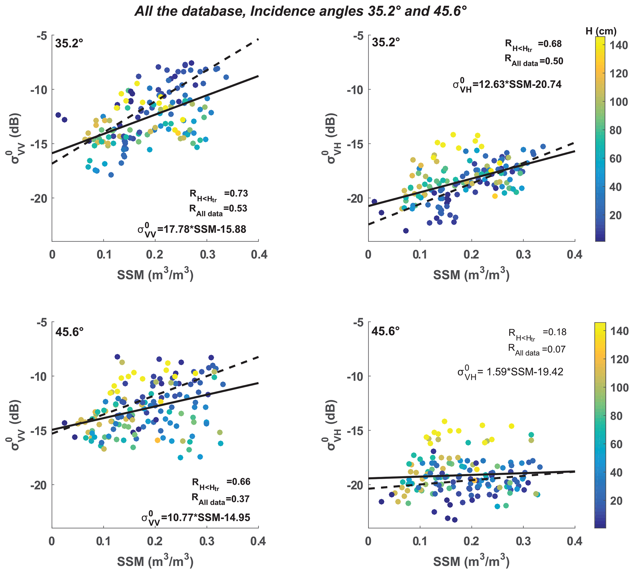
Figure 12 Scatterplots of the relationships between ${\mathit{\sigma }}_{\mathrm{VV}}^{\mathrm{0}}$ and ${\mathit{\sigma }}_{\mathrm{VH}}^{\mathrm{0}}$ and SSM at 45.6 and 35.2 2^∘ angles of incidence. The entire database from the three fields (F1, F2 and F3) is used. H is used to monitor the evolution during the growing season. The significant correlation coefficients are in bold. The solid and the dashed lines correspond to the whole database and data with GLAI < 1.5, respectively.

5 Data availability

This database is archived in DataSuds repository of the French National Research Institute for Sustainable Development (IRD). The database is accessible free of charge with a CC BY license at https://doi.org/10.23708/8D6WQC (Ouaadi et al., 2020a). It can be downloaded as xlsx files accompanied by a variable dictionary containing the variable names and units. The files are also accompanied by metadata including a description of the database, time coverage, keywords and other general information.

6 Conclusion

This paper presents a 3-year database of C-band radar data and all necessary ancillary ground measurements to improve our understanding of the radar signal and to develop inversion methods for land surface parameter retrieval. The data are collected from three heavily monitored wheat fields under semi-arid conditions in the center of Morocco. The database offers a complete set of data for radar applications for wheat monitoring. The measured parameters include fresh and dry aboveground biomass, canopy height, the leaf area index, the cover fraction, surface soil moisture, root zone soil moisture, and surface roughness, in addition to the normalized difference vegetation index and SAR data (the backscattering coefficient and the interferometric coherence). The irrigation and meteorological data are also provided. This database opens up the opportunity to use remote sensing together with measured parameters to understand and investigate the behavior of wheat crops and subsequently to retrieve soil moisture and vegetation variables. The database analysis presented in this paper demonstrates the potentialities of SAR data for wheat monitoring by addressing the well-known sensitivity of SAR to surface soil moisture and vegetation variables. The obtained relationships between SAR measurements including the backscattering coefficient, polarization ratio and interferometric coherence can be used for the application of several backscattering models, the retrieval of biophysical variables and yield prediction in crop models. They can also be useful for land surface models relying on accurate estimation of vegetation height such as the energy balance models (i.e., TSEB, two-source energy balance; Norman et al., 1995). The data set also illustrates the complex signal acquired by C-band radar over wheat crops that is not yet fully understood as it mixes the responses from highly dynamic contributions of soil and vegetation elements. The unique data set provided in this paper should contribute through future studies to improving our understanding of the response of C-band radar observations over annual crops.

Appendix A: Complementary figures

Figure A1 Picture taken over F2 during 2017/18 growing season (14 May 2018) illustrating the specific growing conditions (adventices and stems laid down by wind).

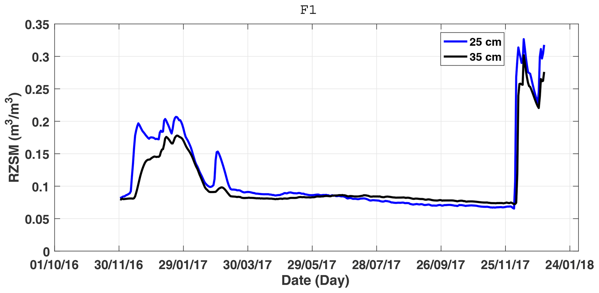
Figure A2 Time series of root zone soil moisture (RZSM) at 25 and 35 cm of depth measured in F1 from 1 December 2016 to 31 December 2017.

Figure A3 Time series of the backscattering coefficient at VV (a) and VH (b) polarizations on F1 at a 35.2^∘ incidence angle during the period from 1 October 2016 to 31 July 2018. The tilling works and phenological stages of wheat are superimposed in panels (a) and (b), respectively. The air temperature, surface soil moisture (SSM), irrigation and rainfall are displayed in panel (c).

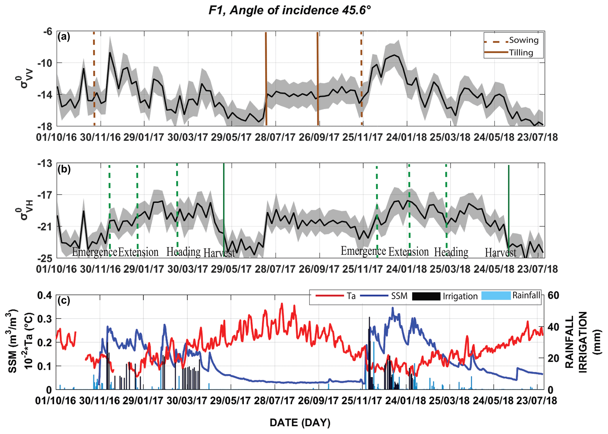
Figure A4 Time series of the backscattering coefficient at VV (a) and VH (b) polarizations on F1 at a 45.6^∘ incidence angle during the period from 1 October 2016 to 31 July 2018. The tilling works and phenological stages of wheat are superimposed in panels (a) and (b), respectively. The air temperature, surface soil moisture (SSM), irrigation and rainfall are displayed in panel (c).

Figure A5 Time series of the backscattering coefficient at VV (a) and VH (b) polarizations on F2 at a 35.2^∘ incidence angle during the period from 1 October 2016 to 31 July 2018. The tilling works and phenological stages of wheat are superimposed in panels (a) and (b), respectively. The air temperature, surface soil moisture (SSM), irrigation and rainfall are displayed in panel (c).

Figure A6 Time series of the interferometric coherence at VV and VH polarizations (a) and the polarization ratio (b) on F1 at a 35.2^∘ incidence angle during the period from 1 October 2016 to 31 July 2018. The tilling works and phenological stages of wheat are superimposed in panels (a) and (b), respectively. The NDVI and measured GLAI are displayed in panel (c). Measured H, FAGB, VWC and AGB are plotted in panel (d). Time series are presented by mean values (solid lines) and standard deviations (shading surrounding the solid lines).

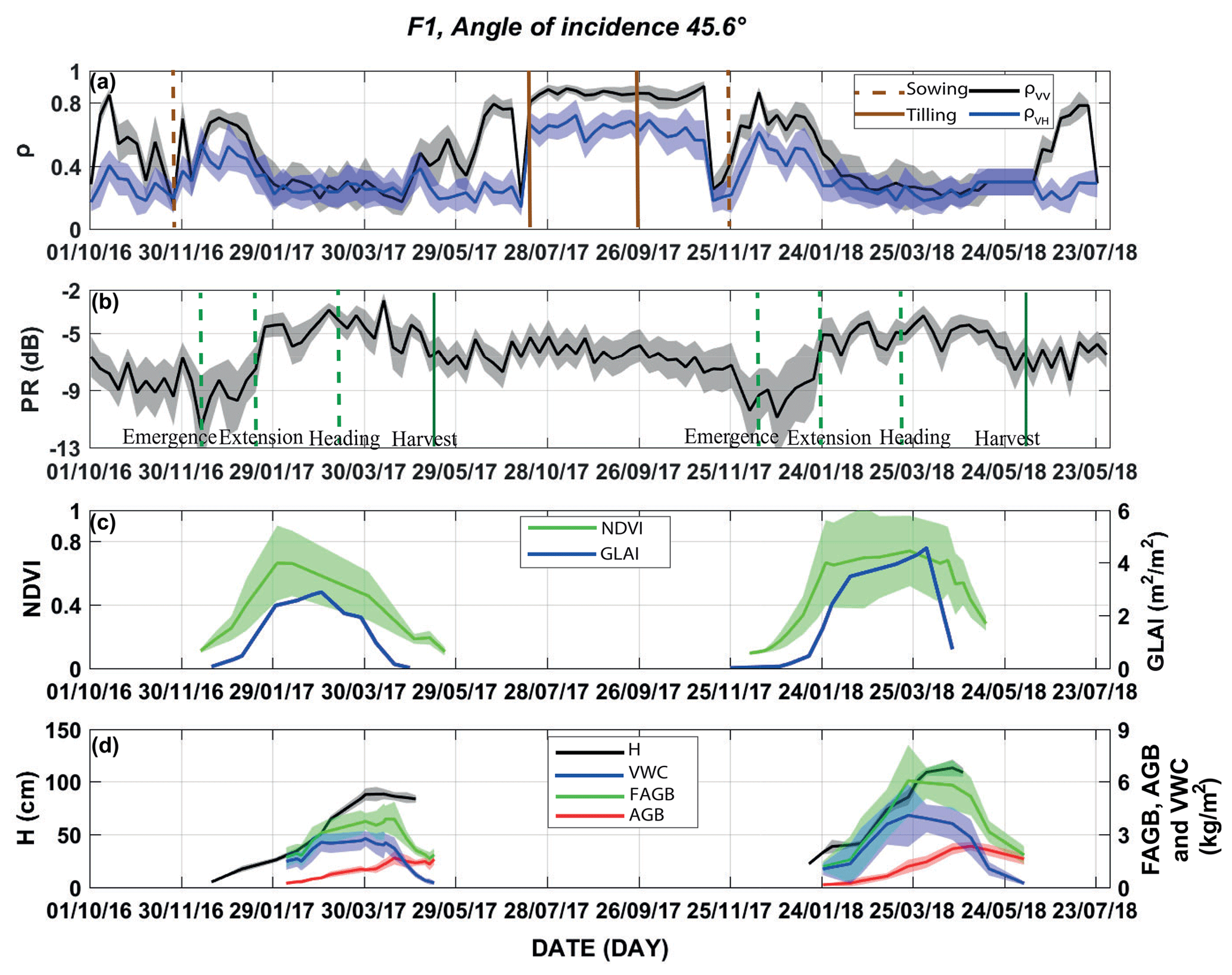
Figure A7 Time series of the interferometric coherence at VV and VH polarizations (a) and the polarization ratio (b) on F1 at a 45.6^∘ incidence angle during the period from 1 October 2016 to 31 July 2018. The tilling works and phenological stages of wheat are superimposed in panels (a) and (b), respectively. The NDVI and measured GLAI are displayed in panel (c). Measured H, FAGB, VWC and AGB are plotted in panel (d). Time series are presented by mean values (solid lines) and standard deviations (shading surrounding the solid lines).

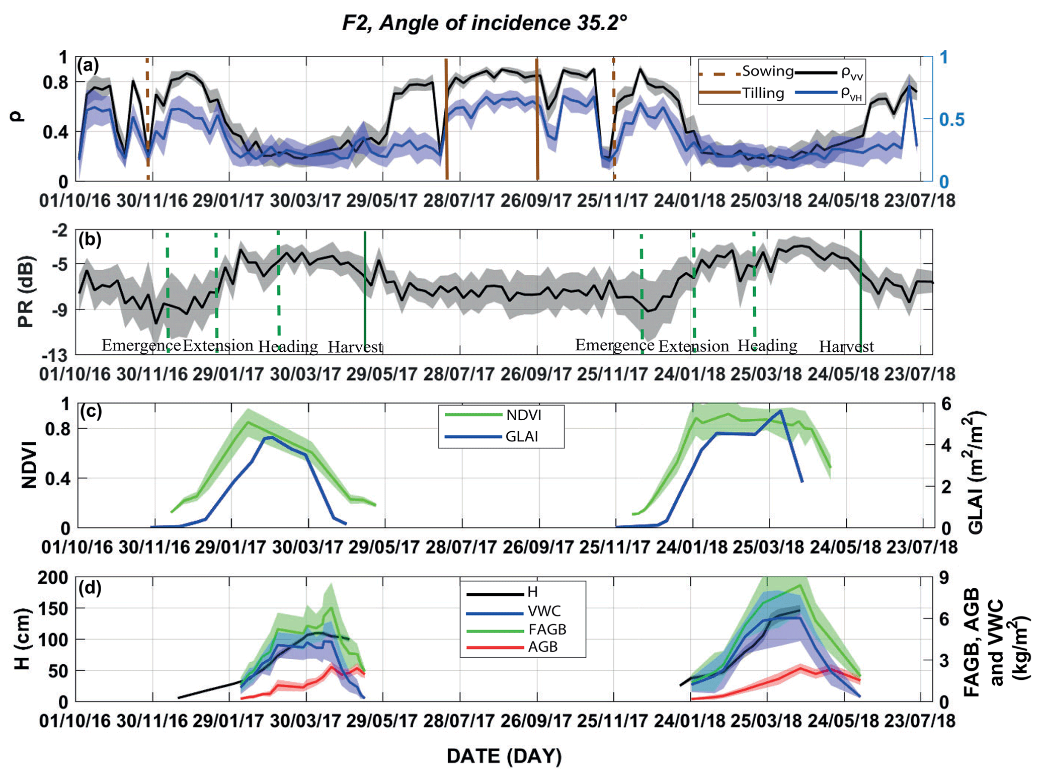
Figure A8 Time series of the interferometric coherence at VV and VH polarizations (a) and the polarization ratio (b) on F2 at a 35.2^∘ incidence angle during the period from 1 October 2016 to 31 July 2018. The tilling works and phenological stages of wheat are superimposed in panels (a) and (b), respectively. The NDVI and measured GLAI are displayed in panel (c). Measured H, FAGB, VWC and AGB are plotted in panel (d). Time series are presented by mean values (solid lines) and standard deviations (shading surrounding the solid lines).

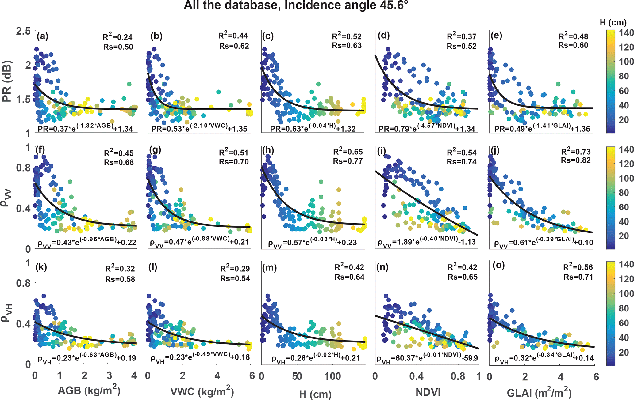
Figure A9 Scatterplots of the relationships between PR; ρ_VV and ρ_VH; and AGB, VWC, H, the NDVI and the GLAI at a 45.6^∘ angle of incidence. The entire database from the three fields (F1, F2 and F3) is used. H is used to monitor the evolution during the growing season. All the determination coefficients (R²) and the Spearman rank correlations (R_s) are significant at 99 %.

Table A1 Details of the field campaigns during the 2016/17, 2017/18 and 2018/19 agricultural seasons. The date format is dd/mm/yyyy.​​​​​​​