The NY-Ålesund TurbulencE Fiber Optic eXperiment (NYTEFOX): investigating the Arctic boundary layer, Svalbard

The NY-Ålesund TurbulencE Fiber Optic eXperiment (NYTEFOX) was a field experiment at the Ny-Ålesund Arctic site (78.9^∘ N, 11.9^∘ E) and yielded a unique meteorological data set. These data describe the distribution of heat, airflows, and exchange in the Arctic boundary layer for a period of 14 d from 26 February to 10 March 2020. NYTEFOX is the first field experiment to investigate the heterogeneity of airflow and its transport of temperature, wind, and kinetic energy in the Arctic environment using the fiber-optic distributed sensing (FODS) technique for horizontal and vertical observations. FODS air temperature and wind speed were observed at a spatial resolution of 0.127 m and a temporal resolution of 9 s along a 700 m horizontal array at 1 m above ground level (a.g.l.) and along three 7 m vertical profiles. Ancillary data were collected from three sonic anemometers and an acoustic profiler (minisodar; sodar is an acronym for “sound detection and ranging”) yielding turbulent flow statistics and vertical profiles in the lowest 300 m a.g.l., respectively. The observations from this field campaign are publicly available on Zenodo (https://doi.org/10.5281/zenodo.4756836, Huss et al., 2021) and supplement the meteorological data set operationally collected by the Baseline Surface Radiation Network (BSRN) at Ny-Ålesund, Svalbard.

1 Introduction

Atmospheric model predictions are either established components of our everyday life – such as weather forecasts – or the subject of vivid scientific, political, and public discussion when it comes to climate projections.

A key quantity in atmospheric models is the transport of heat, momentum, and matter within and across the atmospheric boundary layer (ABL), whose state is most critical for life on Earth. Despite its essential role in the Earth system, the behavior of the ABL is poorly understood for large areas and periods where the boundary layer tends to be stably stratified; therefore, it does not follow similarity theories that apply to the convective boundary layer (CBL) (Sun et al., 2020; Thomas, 2011; Sun et al., 2012; Stiperski and Calaf, 2018; Pfister et al., 2021a; Mahrt, 2010; Acevedo et al., 2014). As a consequence, climate predictions in areas systematically prone to stable boundary layers (SBLs), such as polar regions, suffer from the largest uncertainties – for example, the 2 m temperature, which is highly affected by SBL processes (Holtslag et al., 2013; Davy and Esau, 2014; Stocker, 2014). Therefore, understanding the underlying mechanisms and forcings of key variables is of the utmost importance, as the rate of warming in the Arctic is more than twice as fast as the global average – a phenomenon commonly known as “Arctic amplification” (Cohen et al., 2014; Overland et al., 2016; Davy and Esau, 2014).

A suitable location for conducting SBL research is NY-Ålesund, Svalbard, which is a center for several polar research institutions including the joint French–German AWIPEV station operated by the Alfred Wegener Institute (AWI) and the IPEV (Institut polaire français Paul-Émile Victor). It hosts several long-term observing systems providing complementary observations. Located at 79^∘ N, it experiences long-lived SBLs during the polar night as well as diurnal SBLs during transition seasons.

Under stable weak-wind conditions, classic theories predict turbulence to be totally suppressed by dynamic stability (Monin and Obukhov, 1954). However, a large body of evidence demonstrates that turbulent motions are maintained even for extremely stable conditions (Acevedo et al., 2007; Galperin et al., 2007; Mahrt et al., 2013; Zeeman et al., 2015; Zilitinkevich et al., 2008). This weak-wind turbulence differs greatly from the turbulence dominating the CBL. It covers a broad variety of motions, summarized as submesoscale motions (e.g., Mahrt et al., 2009), which do not correspond to any classic similarity assumption but are significantly nonstationary (Kang et al., 2015; Mahrt et al., 2009).

The fast-evolving, transient, or quasi-stationary nature of submesoscale motions has prompted the development of novel observational systems capable of resolving their temporal and spatial scales: contrary to classic isotropic and homogeneous turbulence, propagation speed and direction of submesoscale motions may differ from those of the mean airflow. Taylor’s hypothesis of frozen turbulence may not be appropriate to translate temporal observations at one point into spatial scales, as ergodicity is often violated (Mahrt et al., 2009; Thomas, 2011). Therefore, to investigate the behavior and motions of the SBL, real spatial observations on an appropriate scale are required (Mahrt and Thomas, 2016). The innovative fiber-optic distributed sensing (FODS) technique (Selker et al., 2006a; Thomas et al., 2012; Pfister et al., 2017) offers the much needed observational capabilities and is at the focus of this unique Arctic field campaign. We deployed a large, horizontal, trapezoidal-shaped, 700 m long FODS array in combination with three vertical profiles at its corners that were about 7 m high to record air temperatures and wind speeds at high temporal (9 s) and spatial (0.127 m) resolution. Using a high-resolution coil-wrapped FODS column (Sigmund et al., 2017), air and snow temperatures were recorded along a 2.5 m vertical profile at subcentimeter resolution. To validate the results and place them in a broader context, FODS observations were complemented by measurements from three sonic anemometers at the corners of the FODS array to collect high-frequency wind measurements, as well as an acoustic wind profiler (minisodar, sodar is an acronym for “sound detection and ranging”) yielding wind statistics between 10 and 300 m a.g.l.

The main objectives of the campaign were as follows

• to investigate the spatiotemporal variability of the stable Arctic ABL during the polar night and shed light on the poorly understood physical mechanisms that drive or determine turbulent and submesoscale motions in the SBL. A deeper understanding will help to find parameters that predict the appearance and character of atmospheric mixing and transport.

• to close the observational gap between point measurements made by the operational infrastructure at AWIPEV and to evaluate their representativeness for different incident flow regimes. The FODS setup was designed to allow the identification, characterization, and tracking of individual atmospheric turbulent and submesoscale motions over several hundreds of meters. Deploying the minisodar also allowed one to close the observational gap between ground measurements from flux towers and operational wind lidar (light detection and ranging) observations, which are available for 150 m a.g.l. upwards.

• to conduct a pilot feasibility study for the technical setup of a large-scale FODS installation in the extreme environment of the Arctic winter.

2 Site description

The experiment was conducted for a period of 14 d from 26 February to 10 March 2020 in Ny-Ålesund ($\mathrm{78}{}^{\circ }{\mathrm{55}}^{\prime }{\mathrm{24}}^{\prime \prime }$ N, $\mathrm{11}{}^{\circ }{\mathrm{55}}^{\prime }{\mathrm{15}}^{\prime \prime }$ E). Ny-Ålesund is one of the northernmost year-round inhabited settlements in the world, located in the Kongsfjord on the west coast of Svalbard's main island of Spitsbergen (see Fig. 1). To the northeast, the village is confined by the fjord, and to the south and west, it is confined by mountains of 500 to almost 800 m a.s.l. (above sea level) as well as several glaciers with their snouts towards Ny-Ålesund.

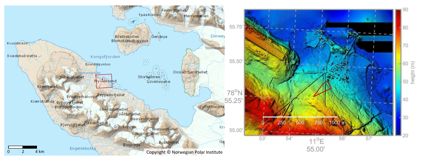
Figure 1 The left panel shows the location of Ny-Ålesund in the Kongsfjord (Copyright © Norwegian Polar Institute, http://toposvalbard.npolar.no, last access: 8 June 2021). The right panel is a visualization of a digital elevation model published by Boike et al. (2018) with the setup marked using a red polygon.

Despite its location at 79^∘ N, Ny-Ålesund experiences relatively mild conditions with mean temperatures varying between −17.0 and −3.8 ^∘C in January and 4.6 and 6.9 ^∘C in July (period from August 1993 to July 2011; Maturilli et al., 2013). These moderate air temperatures are caused by the advection of warm air masses from the Atlantic region (Shears et al., 1998) and the West Spitsbergen Current transporting water from the North Atlantic into the Arctic Ocean, passing Svalbard’s west coast (Aagaard and Greisman, 1975; Haugan, 1999). However, during the measurement period in February and March 2020, Ny-Ålesund experienced very low temperatures down to −30 ^∘C with a mean temperature of −17 ^∘C at 2 m height for the measurement period. The climate of Ny-Ålesund is strongly influenced by polar night and day, which last from 24 October to 18 February and from 18 April to 24 August, respectively (Maturilli et al., 2013). Due to the low solar elevation angle in spring, the mountain ridge south of Ny-Ålesund cast a shadow on the experimental area during the whole field campaign except for very short periods of direct solar radiation on the last days.

The ABL over Ny-Ålesund is determined by the presence of a land–sea contrast, channeling effects induced by the fjord and the topography, and katabatic airflows from mountains and glaciers in the vicinity of the village. The local wind field is driven by orography, resulting in three main wind sectors. The year-round predominant wind directions are southeast and northwest corresponding to the fjord axis with the full range of wind speeds (Maturilli et al., 2013; Jocher et al., 2012; Esau and Repina, 2012, Fig. 1). High wind speeds along this axis result from strong synoptical forcing. The third main wind direction is southwest with wind speeds typically less than 5 m s⁻¹ (Maturilli et al., 2013). Southwesterly winds are associated with katabatic flows down Zeppelin Mountain and the Brøgger Glacier and orographic channeling of the flow by the Brøgger Massif (Schulz, 2017). In wintertime, southwesterly winds are often accompanied by stable stratification and gravity waves excited at low wind speeds (Jocher et al., 2012).

3 Setup

The NYTEFOX experiment was conducted at the southern perimeter of the Ny-Ålesund science station. A picture of the field installation and the settlement taken from Zeppelin station (474 m a.s.l.) and the schematic setup are shown in Fig. 2.

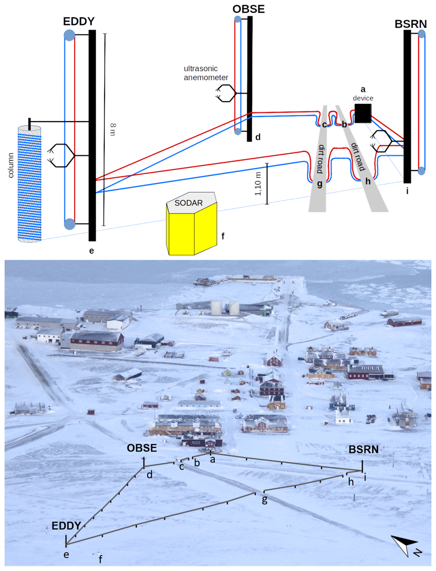
Figure 2 Schematic setup (top panel) and picture of the setup (bottom panel) from the Zeppelin Mountain from the south. The fiber-optic array has a length of 700 m. The letters refer to the locations of the FODS device (a); the road crossings (b, c, g, h); the 10 m towers (d, e, i), and the minisodar (f). The letters a–i refer to the same elements in both panels.

The setup consisted of six main components, which are displayed in Fig. 3, and combined three different sampling techniques: (1) fiber-optic distributed sensing including a horizontal array, and vertical low- and high-resolution profiles yielding air and snow temperature and wind speed (Fig. 3a.1, a.2, a.3); (2) ultrasonic anemometers enabling the computation of atmospheric flux densities using the eddy-covariance technique and other flow statistics (Fig. 3b); and (3) acoustic ground-based remote sensing (minisodar, sound detection and ranging) yielding profile measurements of wind speed and direction and turbulent mixing strength (Fig. 3c). The operational parameters and accuracies for all sampling systems are listed in Table 1. The horizontal, trapezoidal-shaped fiber-optic array had a perimeter of approximately 700 m, whose corners were marked by three 10 m tall towers and the AWIPEV balloon house. The first tower was located near the balloon house and the AWIPEV observatory (referred to as “OBSE” and marked using “d” in Fig. 2), the second tower was located in close proximity to the AWI eddy-covariance station (referred to as “EDDY” and marked using “e” in Fig. 2), and the third tower was south of the AWI meteorological tower at the BSRN field (referred to as “BSRN” and marked using “i” in Fig. 2).

Figure 3 Main components of the NYTEFOX field setup: (a.1) fiber-optic cable (metal encased) – horizontal temperature and wind speed measurements; (a.2) fiber-optic cable (metal encased) – low-resolution vertical profiles of temperature and wind speed across 7 m of height, here at the EDDY tower; (a.3) fiber-optic cable (PVC-coated) – high-resolution vertical temperature profile across the first 2.5 m a.g.l. (column); (b) ultrasonic anemometer – flux densities, wind direction, and wind speed measurements at the towers, here at the BSRN tower; (c) acoustic profiler (minisodar) – wind measurements located near the EDDY tower.

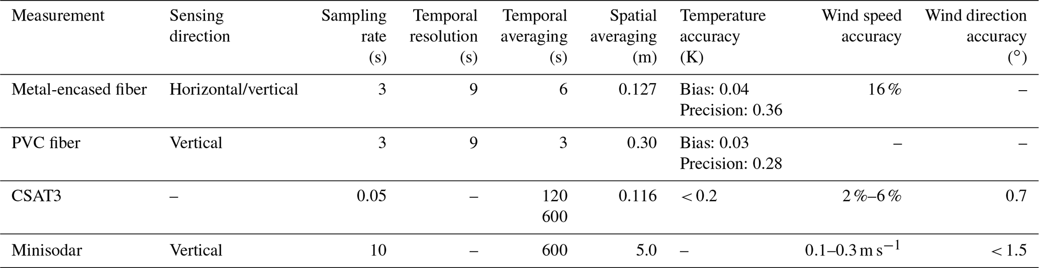
Table 1 Specifications of the measurement techniques: sampling rate, temporal resolution and averaging, spatial averaging, and accuracy of the measurements. The accuracy of the minisodar and CSAT3 wind measurements were taken from their manuals. The accuracy of the CSAT3 temperature measurements was calculated by Fritz et al. (2021). The accuracy of the temperature measured by FODS is based on the readings in the calibration baths: the bias is defined as the standard deviation of the daily averaged differences between the fiber and reference (PT100) temperatures in each bath; the precision is defined as the median of the daily spatial standard deviation of fiber temperatures within each bath. The accuracy of the fiber wind speed is computed as the standard deviation of the fractional absolute deviation of the fiber readings from those of the reference (CSAT3) instrument aggregated to 30 s. The bias systematically depends on the location along the fiber and ranges from an 8 % underestimation to a 13 % overestimation with an average overestimation of 4 %.

Ancillary atmospheric observations of the AWIPEV station complement the abovementioned experiment-specific observational systems. These data include meteorological tower measurements from the Baseline Surface Radiation Network (BSRN) site (Maturilli, 2020a) as well as balloon-borne meteorological data from radiosondes (Maturilli, 2020b).

3.1 Fiber-optic distributed sensing measurements

The fiber-optic distributed sensing (Thomas and Selker, 2021) technique can be utilized to measure the spatial and temporal variability of air temperature and wind speed at a high spatiotemporal resolution. It enables the resolution of short-lived turbulent and longer submesoscale motions in space and time (Peltola et al., 2020; Thomas et al., 2012; Pfister et al., 2019; Zeeman et al., 2015). A main advantage of FODS is that it does not require assumptions regarding spatial homogeneity and ergodicity, as it explicitly resolves thermal and dynamic structures in space and time (Mahrt et al., 2020; Pfister et al., 2021a, b; Zeeman et al., 2015). Therefore, it is a key technology for investigating spatiotemporal phenomena that cannot be observed by traditional meteorological point measurements or their relatively sparse networks.

The sampling principle of the deployed FODS technique is based upon Raman backscattering (see Selker et al., 2006b for details). The frequency-shifted backscatter of a near-infrared laser pulse emitted into a fiber-optic glass core is analyzed for two spectral bands known as Stokes (red shifted) and anti-Stokes (blue shifted). The ratio of their backscatter intensities is proportional to the temperature of the light-scattering portion of the fiber-optic cable, which is why this technique is more commonly referred to as distributed temperature sensing (DTS).

In our setup, the fiber-optic cable was assumed to be in thermal equilibrium with the air and snow temperatures – a reasonable assumption for the low-solar-intensity environment of the polar night – which helps minimize the radiative error (Sigmund et al., 2017). The distance along the fiber-optic cable is resolved by range gating with known values for the speed of light and the length and geometry of the fiber-optic cable. This yields a resolution of 0.127 m along the cable (Table 1) using the highest-resolution DTS device currently on the market (ULTIMA DTS, 5 km variant, Silixa, London, UK).

3.1.1 FODS reference baths

As DTS devices yield only relative temperature measurements, portions of the fiber-optic cables are guided through known and stabilized temperature environments, so-called reference calibration sections, to convert the raw Stokes/anti-stokes ratios into physically meaningful environmental temperatures (Hausner et al., 2011; Van De Giesen et al., 2012; des Tombe et al., 2020). Typically, liquid water baths are used as reference sections in which the fiber-optic cable is loosely coiled while stratification is prevented by mechanical mixing. As liquid water baths are difficult to maintain in the cold Arctic polar night, we deployed a pair of novel solid-state reference baths. Each solid-state reference bath was made up of a 25 kg cylinder of pure copper consisting of four interlocking parts. Their design allowed for an internal groove between a central core and an outer ring to contain several coils of each fiber-optic cable. The temperature of each copper cylinder was thermoelectrically controlled by Peltier elements to within ±0.06 K and observed with two independent high-accuracy platinum resistance (PT-100) thermometers embedded within the copper body next to the fiber-optic cables. The walls of the internal groove housing the fiber-optic cables were painted with a high-emissivity paint (ϵ=0.95) to enhance the radiative transfer between the adjacent solid-state reference parts in order to eliminate thermal differences. Each solid-state reference bath was contained in an insulated portable case to minimize temperature fluctuations in time and across the copper core. One solid-state reference bath was cooled (referred to as “cold bath”) whereas the other was heated (referred to as “warm bath”) to span the range of environmental temperatures observed within the fiber-optic array.

Additionally, an ambient (non-temperature-controlled) reference bath was deployed at the EDDY tower using an insulated plastic case, whose temperature was measured by a high-precision and high-accuracy resistance thermometer (RBRsolo³ T, RBR, Ottawa, ON, Canada). This bath served as an additional reference section at the far end of the PVC-coated fiber (high-resolution vertical profile) only.

3.1.2 FODS measurement components

The key FODS sensor is a pair of two fiber-optic cables, both metal-encased loosely buffered 50 µm single-core fiber (outer diameter 1.12 mm, C-Tube, BRUGG, Switzerland) coated with a 0.2 mm thick polyethylene (PE) white jacket for electric insulation: one actively heated (red fiber in Fig. 2) and one unheated (blue fiber in Fig. 2) fiber-optical cable to obtain wind speed measurements in addition to those of air temperature. The underlying principle of wind speed measurements is the changing temperature difference between both fibers due to convective cooling of the heated cable (see Sayde et al., 2015, and van Ramshorst et al., 2020, for details). As this cooling is sensitive to the angle of attack, only winds orthogonal to the fiber are represented correctly. Therefore, we only obtain relative wind speed information horizontally, and this constraint disappears vertically. Four equally long sections were continuously heated in parallel at a variable heating rate adjusted to environmental conditions (Heat Pulse System, Silixa, London, UK).

The horizontal fiber-optic array was arranged in a trapezoidal shape (see Figs. 2 and 3a.1). The fiber-optic cables were installed at 1.2 m a.g.l. with height being measured at the center between fibers and varying with orography. We chose a two-dimensional array geometry in order to detect the propagation of turbulent and submesoscale structures in all horizontal directions. This was motivated by the frequently changing and meandering wind directions, which are known for weak-wind conditions. The unheated fiber was mounted above the heated fiber at a vertical distance of 0.1 m. Every ≈30 m, tripods were used to support the fiber to avoid excessive sagging. To keep tension on the fiber, clamping fixtures commonly used for pasture fences (see Fig. 3a.1) were mounted at both ends of each section and readjusted when needed. These tensioners were both efficient and relatively easy to deploy in the extreme Arctic conditions.

Using 10 m tall towers, vertical fiber-optic profile observations of air temperature and wind speed (referred to as low-resolution vertical profiles; see Fig. 3a.2) were mounted at three corners of the horizontal array. A total of four fiber-optic sections (heated and unheated, for each upward and downward direction) were secured by plastic disks at the top and at the bottom by horizontal support booms. Due to radiative and mechanical artifacts induced by these support structures, the effective height of the vertical profile decreases to around 7 m (see Sect. 4.1 for the data processing).

The third fiber (see Fig. 3a.3) in the array was an unheated PVC-coated Kevlar-reinforced tightly buffered 50 µm single-core fiber (AFL, Duncan, SC, USA). At the EDDY tower (“e” in the schematic setup in Fig. 2), a high-resolution vertical profile consisting of a 2.5 m high column was used to sample snow and air temperature. The PVC fiber-optic cable was helically coiled around a support structure made from reinforcement fabric (Sigmund et al., 2017), resulting in a subcentimeter vertical resolution (see the data description in Sect. 4.1).

3.2 Ultrasonic anemometers' measurements

Three ultrasonic anemometers (CSAT3, Campbell Scientific, Inc.) were installed at each 10 m tower at approximately 1.4 to 1.5 m a.g.l. and an azimuth angle of about 205^∘ to measure turbulent three-dimensional wind speed components and sonic (acoustic) temperature at a sampling frequency of 20 Hz (see Fig. 3b). For further details on the measurement technique, see Aubinet et al. (2012) and Foken and Napo (2008).

3.3 Minisodar

To observe airflow across the near-surface and lower boundary layer, a heated ground-based acoustic remote sensing instrument (minisodar, sound detection and ranging, SFAS, Scintec AG, Rottenburg, Germany) was set up south of the EDDY tower with an azimuthal orientation of 356^∘ (schematic setup in Figs. 2f, 3c) to measure horizontal wind speed and direction, vertical velocity variance, backscatter intensity, and turbulence kinetic energy from 10 up to 300 m altitude at a 5 m vertical gate resolution (for further details of the basic operation principle, see Neff, 1975). The minisodar was operated in multifrequency mode using eight different acoustic frequencies ranging from 2.4 to 4.8 kHz and provided averaged Doppler and non-Doppler quantities over 10 min increments as output. The minisodar wind profile complements the existing AWI wind lidar (light detection and ranging) system installed on the observatory roof, whose profile observations start at approximately 150 m a.g.l.

4 Data description

In the following, the data processing procedure for each observational system is presented. Observations from all systems are displayed for a 24 h period on 5 March 2020, as this day featured a transition between atmospheric flow and temperature regimes in the early afternoon hours.

4.1 Fiber-optic distributed sensing

The metal-encased fiber (see Fig. 3a.1 and a.2) was attached to the DTS machine via two different optical channels in a double-ended configuration (Thomas and Selker, 2021) such that the observations from the alternating directions were recorded separately. The unheated and heated fibers of the horizontal array, including the low-resolution vertical profiles, were sampled as one optical path by connecting them via a fusion splice in the middle. We recall that each section within this one optical path was routed through the solid-state reference baths, resulting in a total of eight calibration reference sections.

The PVC-coated fiber (high-resolution vertical profile, Fig. 3a.3), which was operated in a single-ended configuration, was calibrated separately, using the two solid-state reference baths and the additional ambient bath at the EDDY tower.

4.1.1 Processing steps

The data processing and fiber calibration was done using the “pyfocs” software package – an open-source Python library from the University of Bayreuth Micrometeorology Group (Lapo and Freundorfer, 2020). The implemented double-ended calibration procedure is based on des Tombe et al. (2020).

The FODS data were converted from length along the fiber (LAF) to a geographically referenced coordinate system. To retrieve this information, several steps had to be performed during and after the measuring period. First, physical locations of all points of interest (e.g., start and end of each defined fiber section) were mapped during the field campaign. Second, artifacts of the fiber holders, street crossings, and edge effects in the calibration sections were removed by employing diagnostics. Artifacts were visible as spatial perturbations in the mean temperature where the fiber was in contact with solid structures, like the fiber holders, due to different heating or cooling from radiation and/or convection. Additionally, these structures subdue the variability in air temperature and, hence, diminish the standard deviation of temperature for adjoining fibers. In an iterative process, the section margins were manually adjusted, discarding as little FODS data as possible. Third, all unheated and heated fiber sections were spatially aligned by finding the maximum spatial cross-correlation when no heating was applied. The necessity for this arises from the wind speed derivation, which requires the paired fibers to be spatially aligned. Due to strong vertical gradients, even small mismatches in the vertical coordinate on the order of a single LAF bin strongly reduces the data quality. Fourth, the aligned temperatures were mapped to physical geographic coordinates (UTM, with the z coordinate being height a.g.l.) by interpolating the values obtained for the start and end points of each fiber-optic section. As a last step, data were temporally resampled to an evenly spaced time step of 9 s to eliminate small deviations in integration times by the internal signal processing in the DTS device.

4.1.2 Corrections

Due to deployment-specific technical difficulties in the cold solid-state calibration bath, its temperature slowly drifted over time, rendering FODS observations implausible whenever the temperature differences between warm and cold baths were small or even reversed. Hence, a criterion for quality control was established: 2 min temporal averages of the sonic temperature were compared to the most closely co-located FODS section in the three vertical low-resolution profiles. Sonic temperatures were converted into dry-bulb temperatures, using slow response humidity data from the Baseline Surface Radiation Network (Maturilli et al., 2013). The fiber temperature was spatially averaged over 1 m centered at the ultrasonic anemometer mounting heights for each profile for the ascending and descending branches of the unheated fiber, resulting in a spatial average over 14 bins. Next, the first approximate derivative of the temperature difference (the change in difference between each 2 min interval) between the FODS and sonic temperatures was calculated and averaged across all three towers. All data exceeding $\left|\mathrm{0.61}\right|$ K per 2 min, defining the upper 99th percentile, were rejected. To avoid small data snippets, data between the resulting gaps were rejected if they were shorter than 1 h 17 min, which was the minimum duration needed for scientific interpretation in subsequent data analysis. A total of 20 h 50 min of data were excluded from the fiber-optic data set for both the metal-encased and PVC-coated fiber.

The bottom of the high-resolution profile (column, PVC-coated fiber) was immersed in snow of varying density due to uneven snow drift and compaction, resulting in substantial horizontal heterogeneity across the cross-section of the column. The heterogeneity manifested itself as systematic alternating stripes of warmer and colder temperatures across each coil. To eliminate this artifact in snow temperatures, only the side of the column where the signal was most strongly uncorrelated with air temperatures above the snow surface was retained. This step led to an effective coarser vertical resolution in the snow of 10 mm instead of 2.5 mm in the lowermost aerial section.

4.1.3 Final data

All provided fiber-optic data have a temporal resolution of 9 s. The sampling resolution is 0.127 m for the metal-encased fiber. The sampling resolution of the PVC fiber used for the high-resolution column was 0.254 m along the fiber, but the coil wrapping yielded a much higher effective vertical resolution of 2.5 mm in the lowest quarter (0 to 0.625 m), 5 mm from 0.625 to 1.25 m, 10 mm from 1.25 to 1.875 m, and 20 mm from 1.875 to 2.5 m. The effective vertical resolution was varied due to the logarithmic nature of vertical temperature and wind speed gradient close to the surface.

In the following, we present the observations for the 5 March 2020 as an example for the FODS temperature between the OBSE and EDDY towers (Fig. 4). Figure 4a displays the entire 24 h period, covering a distinct temperature regime change around 15:00 UTC. The two temporal subsets below illustrate the different character of structures during a strong-wind (Fig. 4b) and weak-wind (Fig. 4c) regime, showing the unique capabilities of true spatiotemporal observations. As the different regimes go along with characteristic wind direction patterns, the direction at both towers is additionally plotted in Fig. 4.

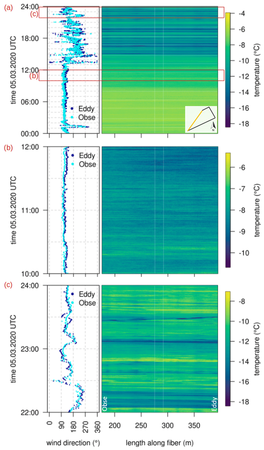
Figure 4 Fiber-optic temperature along the OBSE–EDDY transect and the ultrasonic anemometer wind direction (temporal resolution =30 s) at the OBSE and EDDY towers for the whole day on 5 March (a) and for two 2 h subsets during the strong-wind regime in the morning (b) and weak-wind regime at night (c).

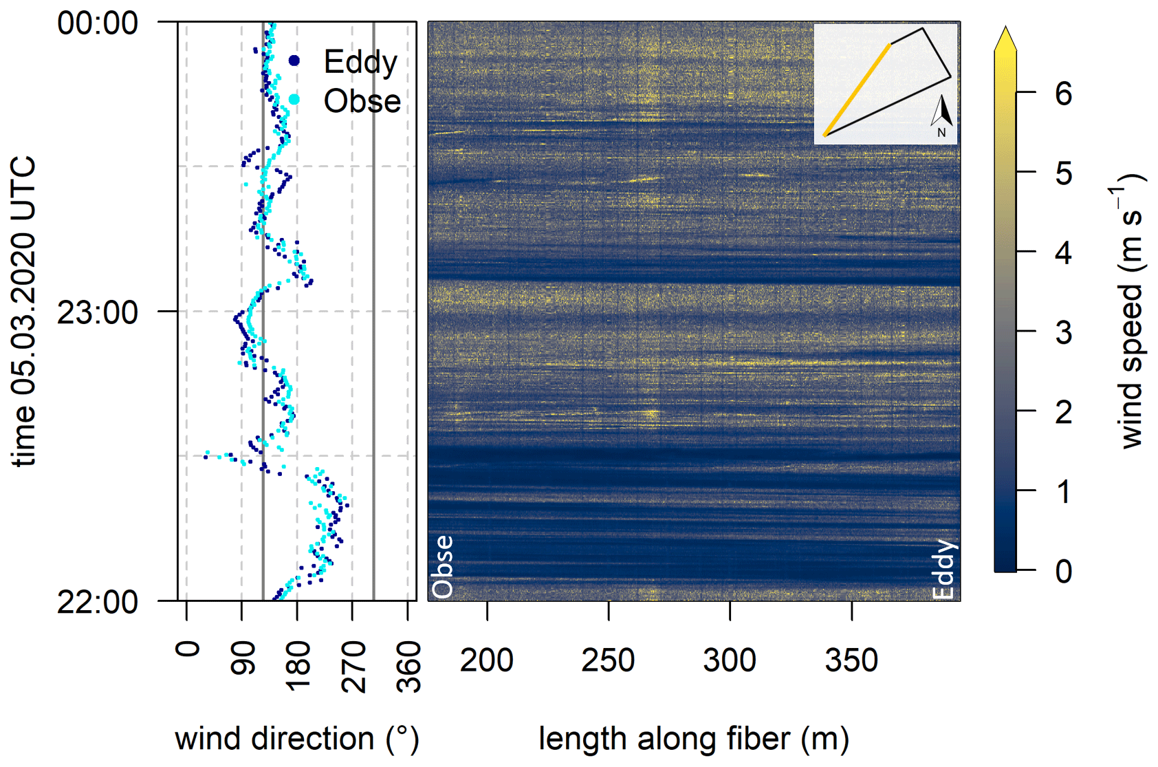
Figure 5 Fiber-optic wind speed along the OBSE–EDDY transect for the 5 March. For visualization purposes, some of the stronger artifacts created by fiber holders and marking tape (appearing as vertical lines) were removed using spatial interpolation. The heating rate for this period was 1.6 W m⁻¹. The left panel shows the ultrasonic wind direction (temporal resolution =30 s) at the OBSE and EDDY towers. Gray vertical lines indicate the wind directions orthogonal to the fiber, where wind speeds are not biased by the angular dependence of the method.

During the morning, temperatures were mostly uniform in space and time due to the intense shear-driven mixing as a result of high wind speeds (see Fig. 7). After the breakdown of the strong winds around 13:15 UTC and the first meandering at this time, it takes almost 2 h for the temperature to drop and characteristic weak-wind, submesoscale structures to dominate. The latter appear as oscillating wind direction and strong temperature nonstationarities that start around 15:00 UTC. The observed oscillations in both speed and direction are a typical submesoscale phenomenon called meandering (Anfossi et al., 2005; Mahrt et al., 2009). Especially the wind direction shift from the southwest to the east-northeast between 22:00 and 22:30 UTC, which exceeded 180^∘ in magnitude, caused the passage of cold-air structures. The dramatic temperature drop of almost 10 K during its passage suggests that it was katabatic outflow originating from the Brøgger glacier that is situated southwest of the measurement site.

The visualization proves that submesoscale motions during weak-wind situations can be resolved and tracked with FODS, as aimed for in the second objective outlined in Sect. 1.

The distributed wind speed observations for the abovementioned temporal weak-wind subset (Fig. 5) indicate a coherence between temperature and wind patterns. While low temperatures mostly go along with low orthogonal wind speeds (cf. Figs. 4c and 5), this implies either overall low velocities or a change in wind direction due to the directional dependence of the measurement technique (see Sect. 3.1.2; Pfister et al., 2019; van Ramshorst et al., 2020). Overall, variability is higher in time than in space. However, there are still periods during which winds varied spatially across the displayed section, such as the passing atmospheric feature around 23:30 UTC.

The regime change between a strong-wind and a weak-wind regime observed horizontally in Fig. 4 was also clearly articulated in the vertical FODS profiles (Fig. 6). This change caused an abrupt transition from isothermal to strongly stably conditions, with a surface-based inversion that is captured especially by the high-resolution vertical column (right graph). Note that the lower 0.23 m of the column was immersed in snow, which results in higher and more homogeneous temperature values.

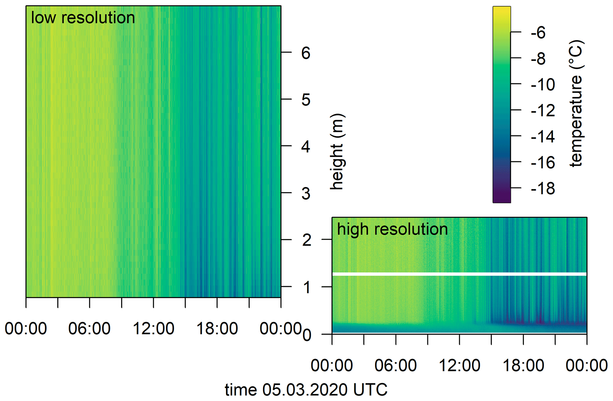
Figure 6 Low-resolution vertical temperature profile at the EDDY tower (left graph) and the high-resolution temperature profile across the first 2.5 m a.g.l. (column) at the EDDY tower (right graph) for the 5 March 2020. The white stripe in the right plot results from rejected data where the fiber was in contact with a plastic support ring.

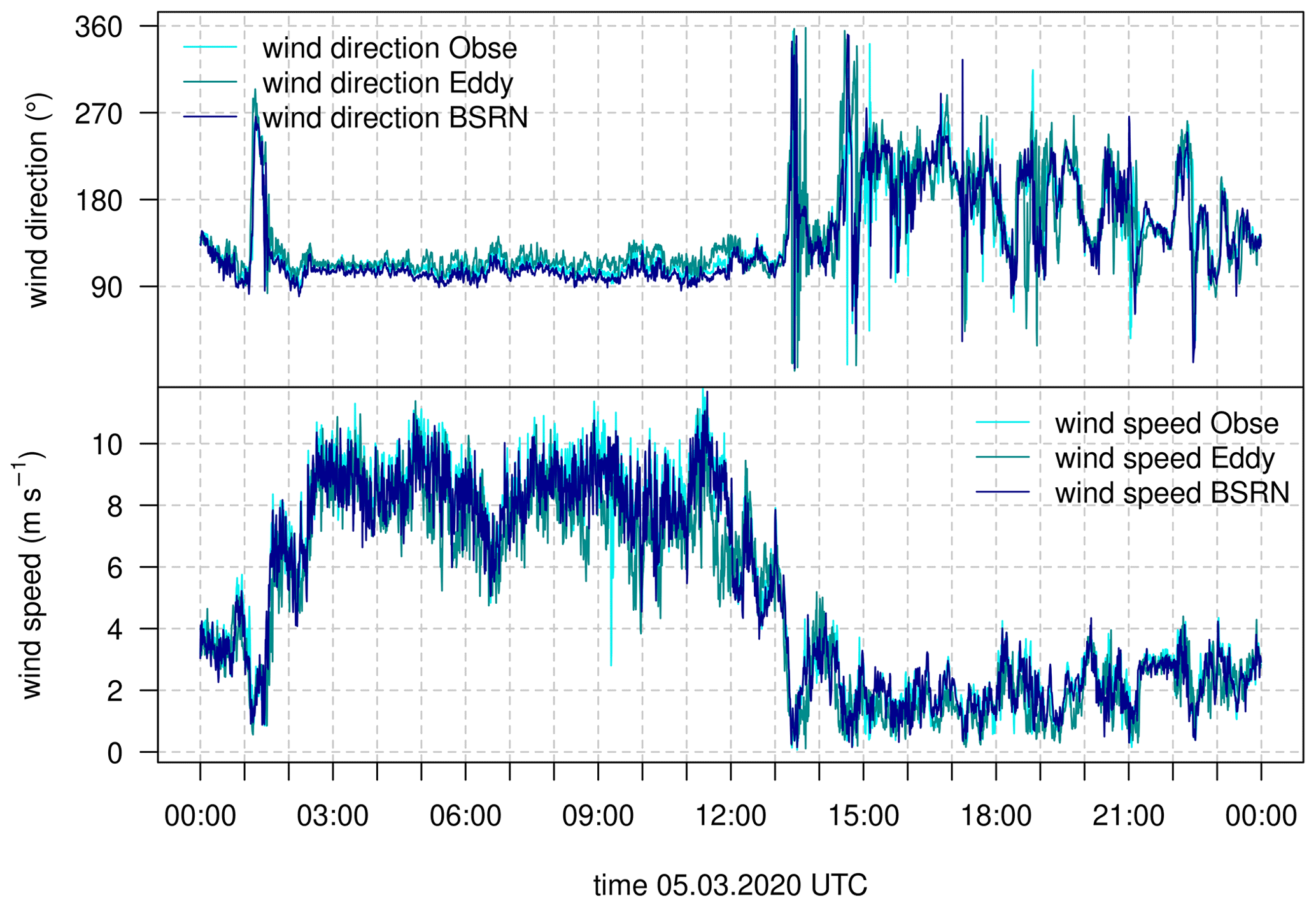
Figure 7 Wind direction and wind speed (temporal average 30 s) for all three ultrasonic anemometers at the three towers (OBSE, EDDY, and BSRN) for the 5 March.

4.2 Ultrasonic anemometers

Eddy-covariance fluxes from sonic anemometers located on the three towers were computed using fixed perturbation timescales of 30 s and subsequently averaged to 2 min using the “bmmflux” software tool of the Micrometeorology Group of the University of Bayreuth (see the Appendix in Thomas et al., 2009). First, the raw data were filtered according to instrument flags and plausibility limits. Subsequently, unphysical turbulence data were removed using a despiking routine (Vickers and Mahrt, 1997). A three-dimensional rotation routine was applied aligning the flow for each averaging interval into the horizontal along- and cross-wind components and eliminating the mean vertical component potentially caused by a tilt in the ultrasonic anemometer, surface conditions, or semi-stationary eddies of timescales exceeding the perturbation timescale (Wilczak et al., 2001). Computed fluxes were corrected for low- and high-pass losses following Moore (1986). The buoyancy flux was converted into sensible heat flux by a post hoc buoyancy correction (Liu et al., 2001). Quality flags for turbulent fluxes were computed according to Foken et al. (2004) and applied to discard data either not satisfying stationarity or compliance with similarity theory. The scheme runs from 1 (best quality) to 2 (worst quality), and we discarded data with flags >1. For the 2 min data triple-order moment variables are computed. A comprehensive list of bmmflux output statistics is provided as part of the data repository. The ultrasonic anemometer wind speed and wind direction are consistent with the regime change observed in the FODS data (Fig. 7): the near-surface easterly airflow starts to decrease in strength around noon, reaching a first minimum of ≤ 1 m s⁻¹ around 13:30 UTC. The calmer winds with speeds ranging from 0.5 to 4 m s⁻¹ came predominantly from southwest, interrupted by sudden distinct wind direction shifts.

4.3 Acoustic profiler (minisodar)

Raw acoustic backscatter at all eight frequencies from each acoustic pulse were subject to quality control using the built-in instrument filtering routines for spectral width, ground clutter, signal-to-noise ratio, and plausibility limits. Quality-filtered data from all frequencies were then combined to compute vertical profiles of the horizontal wind speed and direction, vertical velocity variance, turbulence kinetic energy, and backscatter intensity over an averaging interval of 600 s (Fig. 8).

Identical to the changes found in the FODS and sonic anemometer measurements, the regime shift in wind speed and direction was also observed by the acoustic profiler. However, the profiler observations limit the distinct regime change in wind direction (east-southeast to southwest) after 13:30 to a maximum depth of ≤ 80 m a.g.l. Flow further aloft remained easterly showing common boundary-layer profiles with a logarithmic increase in wind speeds of up to ≈ 8 m s⁻¹. This supposedly larger-scale synoptic flow was interrupted by shorter, approximately 1 h long periods of very weak westerly winds beyond 140 m a.g.l. The vertical directional shear characteristic for these interruptions suggests that strong vertical decoupling and strongly stable near-surface temperature gradients are required to maintain the decoupling in spite of relatively strong southwesterly surface winds of up to 4 m s⁻¹ (see Fig. 7). The depth of the katabatic cold-air intrusion from the Brøgger Glacier between 22:00 and 22:30 UTC was restricted to the lowest 30 m a.g.l. and characterized by a calm period throughout the observation layer. This example period emphasizes the role of local topography as source areas for local flows and submesoscale motions when the synoptic forcing is negligible. Deriving such potential drivers of submesoscale motions addresses the first objective of the experiment, as outlined in Sect. 1. The varying maximum measuring height (missing data displayed in gray) was caused by low clouds, snowfall, and wind noise around the acoustic enclosure during the strong-wind period.

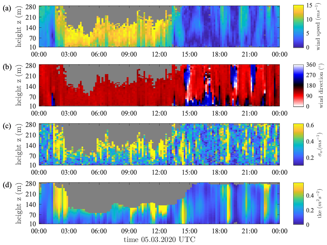
Figure 8 Time–height plots (sodargrams) observed with the minisodar data on 5 March 2020: (a) horizontal wind speed, (b) horizontal wind direction, (c) standard deviation of the vertical wind velocity σ_w, and (d) turbulence kinetic energy (tke). Each pixel represents an average over the gate height of 5 m and a period of 10 min. Missing data are displayed in gray.

5 Data availability

The data available from all observational systems for the NYTEFOX campaign period in February and March 2020 are summarized in Fig. 9. Gaps in the records were caused by instrument failure and post-field data processing, as described in Sect. 4.1. The FODS data files containing actively heated fiber temperatures (used for wind speed computations) in the Zenodo repository include data from a period when heating was only working intermittently or was at non-optimal heating rates (start to 27 February 2020, 18:44 UTC). After 27 February 2020 at 18:45 UTC, all heating issues were resolved, and this period offers the best data quality (as indicated in Fig. 9).

The complete data set is available on Zenodo: https://doi.org/10.5281/zenodo.4335461 (Huss et al., 2021). The Python library “pyfocs”, used for processing and calibration of the fiber-optic data (see Sect. 4.1.1), can also be retrieved from Zenodo via https://doi.org/10.5281/zenodo.4292491 (Lapo and Freundorfer, 2020).

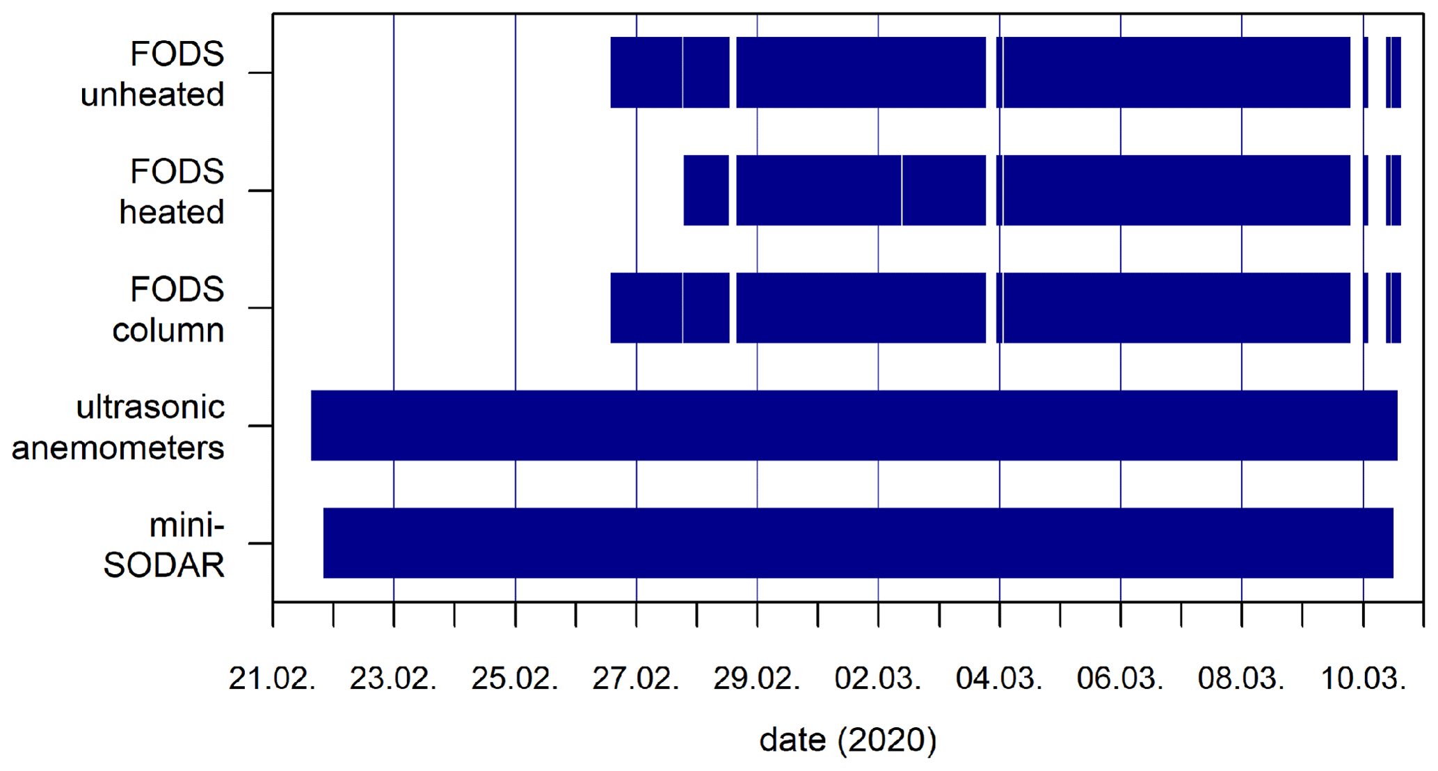
Figure 9 Data availability of the different NYTEFOX data sets for the campaign period in February and March 2020.

6 Summary and outlook

The NYTEFOX field campaign yielded a unique near-surface and boundary-layer meteorological data set for the Arctic polar night above land, which, for the first time, combines observations from fiber-optic distributed temperature and wind sensing, sonic anemometry, and acoustic profiling in this environment. This combination allowed for unprecedented detail in observing the horizontal and vertical thermal and dynamic structure across the land–snow–air continuum. These data can be used to explore the role of submesoscale motions on the SBL in the Arctic. Our complementary setup provides the unique ability to observe the role of topography in processes such as the interactions between katabatic outflows from the surrounding glaciers and the synoptic-scale flow over the Svalbard archipelago. The data allow for the identification of the horizontal and vertical scales of turbulent and submesoscale structures and their trajectories. The first interpretation of findings supports the dominant role of any topographic variation – at a scale ranging from decimeters to hundreds of meters – in airflow and near-surface transport when flows and turbulent transport are sufficiently weak, solely enabled by distributed sensing.

One goal of the NYTEFOX campaign was to provide a proof of concept for future applications of the horizontal fiber-optic distributed sensing technique in similarly challenging environments. While the feasibility of FODS has been proven for midlatitude boundary layers (Thomas et al., 2012; Sayde et al., 2015; Peltola et al., 2020; Schilperoort et al., 2020; Pfister et al., 2021a), the high-quality FODS data and their physical consistency with other more traditional near-surface meteorological observations underline the technical feasibility and the functionality of FODS deployments in extreme temperature and wind conditions of the polar regions. Note that temperatures during the measuring period dropped to −30 ^∘C with an average of −17 ^∘C, which is extraordinarily cold for NY-Ålesund and more representative of the higher Arctic. Therefore, this innovative observational technique has unique merit to complement future boundary-layer studies (even in challenging environments) to observe motions and transport in a spatially resolving fashion across interfacial boundaries.