the Creative Commons Attribution 4.0 License.
the Creative Commons Attribution 4.0 License.
 | 13 Jul 2021
A mean-sea-level pressure time series for Trieste, Italy (1841–2018)
Fabio Raicich
Renato R. Colucci
A time series of mean-sea-level pressure was built from observations performed in Trieste from 1 January 1841 to 31 December 2018. Original historical documents provided information on the instruments and on the observation sites. Mercury barometers have always been available. Until 1877 they represented the only instruments in operation, while from 1878 onwards barograph records became available. The time series consists of mean daily values that were computed from 24-hourly data, when possible, or otherwise adjusted to 24 h means on the basis of climatological daily pressure cycles. The time series was homogenized on the basis of the available metadata, reducing pressure to 0 ∘C and to mean sea level. Basic quality checks were applied, including the comparison with pressure time series from nearby stations. As a result, the data prior to 1865 turned out to be suspect. A mean-sea-level pressure trend of 0.5 ± 0.2 hPa per century was estimated for the 1865–2018 period. The data are available through PANGAEA (https://doi.org/10.1594/PANGAEA.926896; Raicich and Colucci, 2021).
- Article
(6777 KB) - Full-text XML
- BibTeX
- EndNote


Long time series of environmental observations represent key elements for climate studies.
In the last decades, significant efforts have been made in Europe to recover long meteorological time series, among which those of the atmospheric pressure. Quality-checked and homogenized time series of daily pressure data were produced for several European cities in the framework of the IMPROVE project, extending from the mid-18th century to the 1990s (Camuffo and Jones, 2002). Pressure data for various sites of the Po Plain, in Italy, were recovered by Maugeri et al. (2004). More recently, Cornes et al. (2012a, b) reconstructed over 300-year-long time series for London and Paris, respectively. A comprehensive global inventory of pressure time series that started before 1850 can be found in Brönnimann et al. (2019).
In Trieste, regular observations of the atmospheric pressure and the air temperature were reported to start in 1788 (Rossetti, 1829); however, only sparse data are available for the period before 1802. Since then, the observations have been performed regularly. The earlier observations are only available from local newspapers, while data from 1841 onwards can be found in original manuscripts that are held in the archives of the Institute of Marine Sciences of CNR (CNR-ISMAR) in Trieste (Italy).
This paper focusses on the reconstruction of a daily mean-sea-level pressure time series from 1841 to 2018 using the original observations and the information on the instruments and their heights above mean sea level.
In the next section, the data used in this work will be described, together with their sources and the instruments. The methods used to derive the daily mean-sea-level pressure will be outlined in Sect. 3. Section 4 will include basic information on the data availability. Concluding remarks will be summarized in Sect. 5. Technical details on the barometer corrections and the trend estimates will be presented in Appendices A and B, respectively.
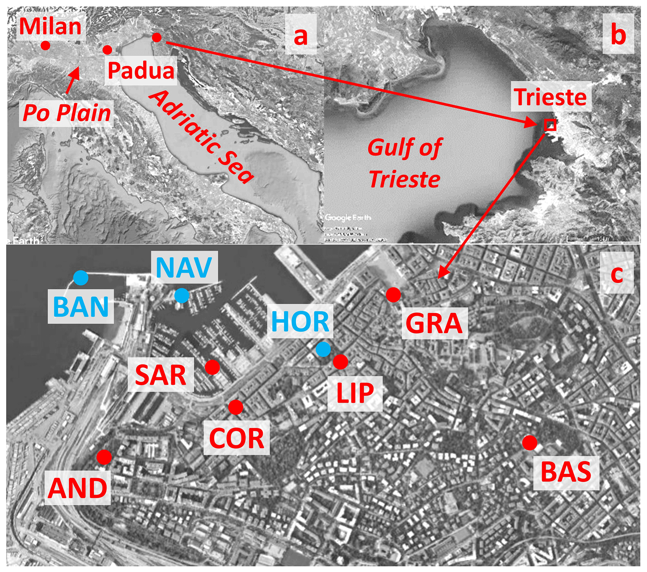
Figure 1(a) The Adriatic and Po Plain regions. (b) The Gulf of Trieste. (c) Aerial image of Trieste. The observation sites whose data are relevant for this study are displayed in red; other sites cited in the text are shown in light blue. (Images extracted from © Google Earth; © 2020 Landsat/Copernicus, © 2020 CNES/Airbus, © 2020 Digital Globe, © 2020 TerraMetric.)
2.1 Overview
Pressure observations were initially performed under the responsibility of the local institution committed to the education of future seamen. It operated under different denominations until 1898, namely the Nautical School (Scuola di Nautica) until 1812, the Royal and Nautical Academy (Accademia Reale e di Nautica) from 1817 to 1844, and the Commercial and Nautical Academy (Accademia di Commercio e Nautica) until 1878; in that year the meteorological and the astronomical observatories of the academy were merged into the Maritime Observatory (Osservatorio Marittimo). In 1898 the new Astronomical-Meteorological Observatory (Osservatorio Astronomico-Meteorologico), independent of the academy, was established. In 1904, the name was changed back to Maritime Observatory, which was renamed Geophysical Institute (Istituto Geofisico) in 1919 and subsequently Thalassographic Institute (Istituto Talassografico) in 1941. Finally, in 2002, the latter became part of the newly established Institute of Marine Sciences (Istituto di Scienze Marine) of the Italian National Research Council.
Until 1812, the observations were performed in the Public Library situated in the Grand Square (piazza Grande, GRA, Fig. 1c). A second-order meteorological station was established in 1817 (Osnaghi, 1886) on the premises of the Royal and Nautical Academy in Leipzig Square (piazza Lipsia, LIP, Fig. 1c). In 1841, a new observatory was set up in the same building. In 1868, the meteorological station and service were reorganized. In the first half of that year, a new temporary station, located in another room and with new instruments, was operated in parallel with the old one. A fully equipped observatory was finally established on the first floor in July 1868, and the old one was discontinued. Probably in 1868, but certainly before 1884, the observatory became a first-order station (Osnaghi, 1886). In 1870, the station was relocated to the third floor and, finally, in 1876 to a new room on the roof. In 1903, the whole observatory was moved from Leipzig Square, not far from the harbour, to Villa Basevi (BAS, Fig. 1c), on a nearby hill, and it was equipped with new instruments. In February 1920, the station was relocated to Sant'Andrea (AND, Fig. 1c), again in the low-lying part of the city near the harbour. On 10 June 1944, the building hosting the station partially collapsed due to an aerial bombing and, as a consequence, the barograph and the control barometers were moved to the university premises in Corsica Street (via Corsica, COR, Fig. 1c). In August 1950, the instruments were relocated to the previous site (AND) in the rebuilt institute, and they remained there until the beginning of January 2019, when the station was moved to Molo (pier) Sartorio (SAR, Fig. 1c). The positions of the observation sites are summarized in Table 1.
Table 1Summary of the observation sites shown in Fig. 1c, their geographical positions (from Google Earth), and the time intervals when the observations were made.
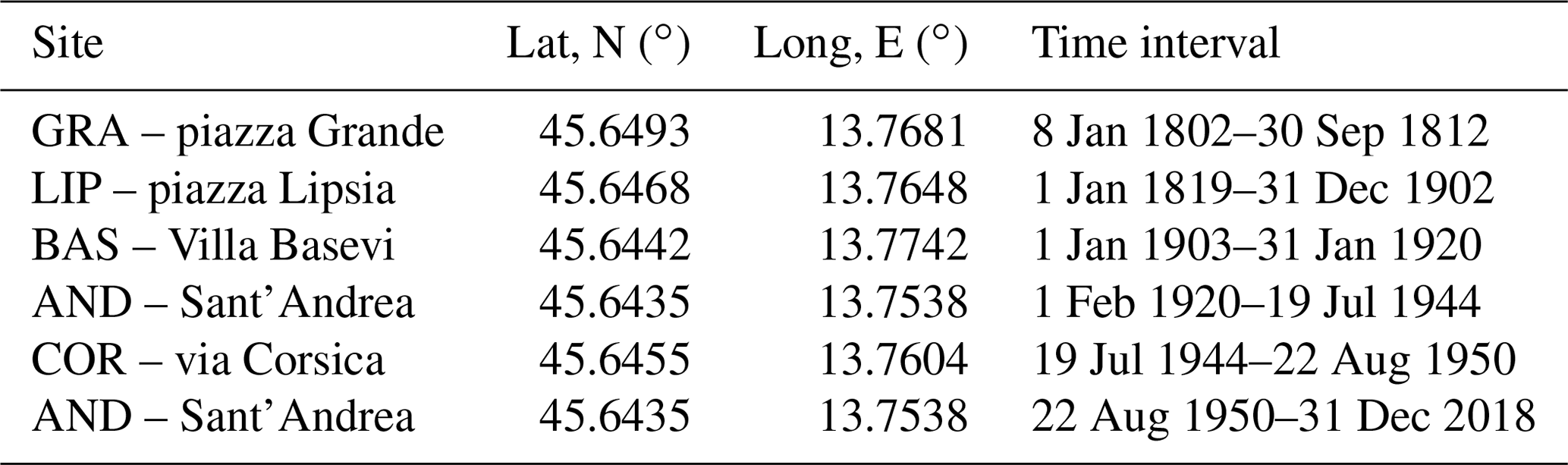
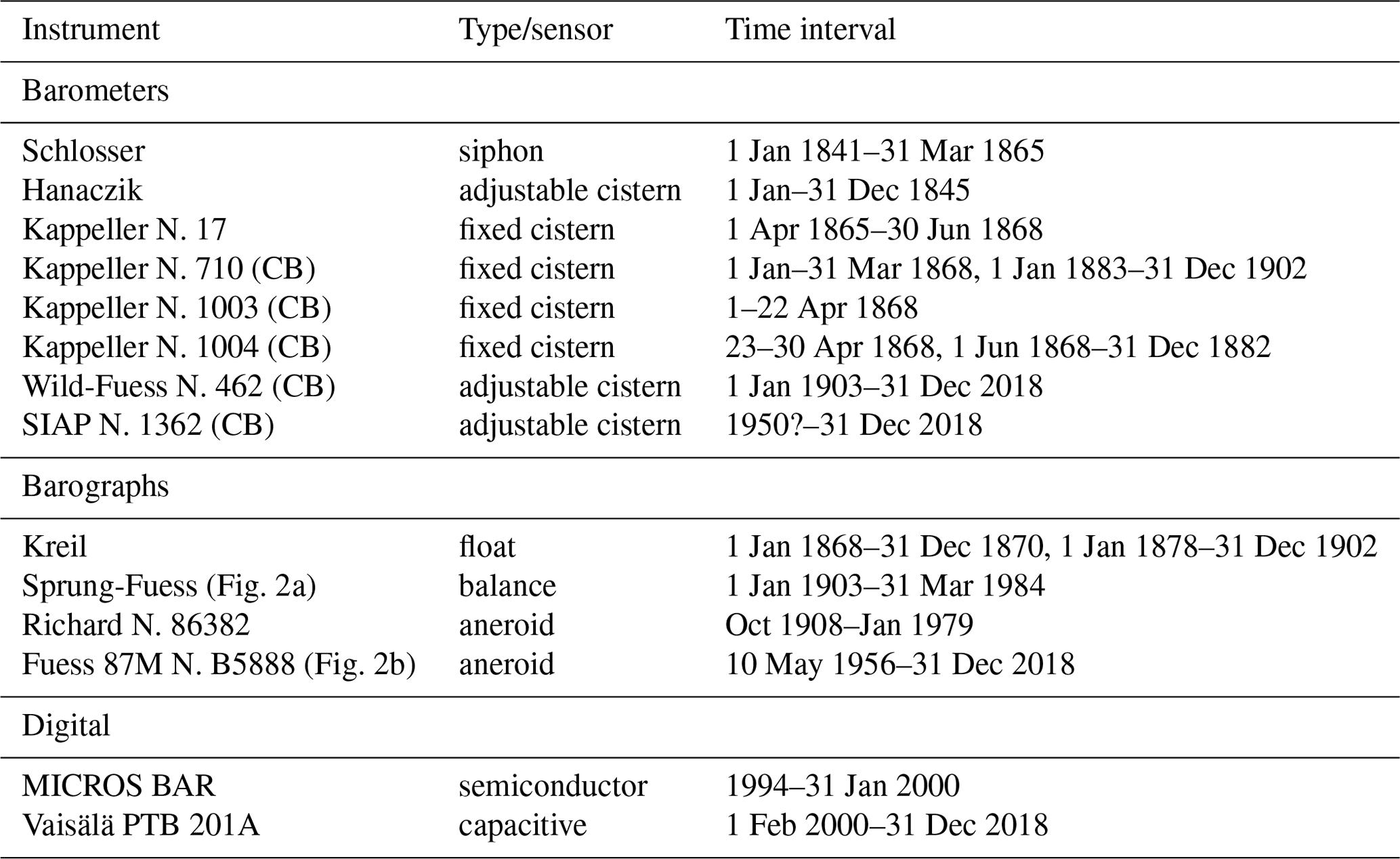
Table 2Summary of the instruments used for the observations. Those indicated with “(CB)” were also used as control barometers for the barographs.
For the sake of completeness, we should mention other meteorological stations where atmospheric pressure is being measured in Trieste, namely: Molo (pier) Fratelli Bandiera (BAN, Fig. 1c), managed by the Civil Protection of Friuli Venezia Giulia Region (since 1994); piazza Hortis (Hortis Square, present name of Leipzig Square, HOR, in Fig. 1c), managed by the Nautical Technical Institute and the University of Trieste (since 1993); Molo (jetty) Lega Navale (NAV, Fig. 1c), managed by the Istituto Superiore per la Protezione e la Ricerca Ambientale (Superior Institute for the Environmental Protection and Research) since 1998.
Data prior to 1841 can only be found in the local newspaper L'Osservatore Triestino, which in January 1802 started publishing the observations of pressure, temperature, and the “state of the sky”, namely cloudiness and precipitation. The publication of meteorological data was rather regular until 1808 then increasingly irregular until September 1812 when it ceased; it was resumed in January 1819 and continued regularly except for occasional interruptions.
Original meteorological records and summaries have only been available since January 1841; they are held in the archives of CNR-ISMAR. The data from 1 January 1841 to 30 June 1868 were collected in seven handwritten volumes, named Repertori (Gallo, 1841–1868). Subsequently, the direct meteorological observations were summarized on monthly data sheets. When automatic recording instruments became available, hourly data were also tabulated on a monthly basis.
Note that the unavailability of any data before 1802 and of the original observations until 1840 was already stated by Gallo (1846). The second part of this statement is surprising because he took over the responsibility for the observations on 1 January 1841, but he seemed unaware of the activity performed in the very same place until 31 December 1840. Moreover, he explicitly said that the barometer used in 1841 had also been used previously (Gallo, 1841–1868, 1846).
2.2 The instruments and the observations
Mercury barometers were available during the whole 1802–2018 period, while barographs were used in 1868–1870 and from 1878 onwards. The station was always equipped with at least one control mercury barometer that was checked against a standard barometer (also named Normal Barometer). Barograph records were always calibrated by means of the observations made with a control barometer. Three types of mercury barometer were used, namely siphon (Gay-Lussac type), with adjustable cistern (Fortin type), and with fixed cistern (Kappeller type). In order to obtain the atmospheric pressure in standard conditions, that is 0 ∘C temperature and mean sea level (MSL), the observations require appropriate corrections, described in Appendix A.
The original data sheets and summaries generally reported the essential information on the barometers in use, namely model and manufacturer, and height above MSL. Table 2 summarizes the instruments from which the pressure data used in this study were obtained, as retrieved from the original documents and from review works (Mazelle, 1889, 1907; Polli, 1951–1952; Stravisi, 2006). Unfortunately, the 1802–1840 period lacks metadata, namely the barometer location, height, and temperature; therefore, those data were excluded from further analyses.
Three direct measurements of the atmospheric pressure were made with the control barometer (Table 2) in the morning, in the early afternoon and in the evening, namely at 07:00, 14:00, and 22:00 from 1 January 1841 to 30 June 1868, then at 07:00, 14:00, and 21:00 until 31 December 1918, at 09:00, 15:00, and 21:00 until 31 March 1920, at 08:00, 13:00, and 18:00 until 7 April 1927, and at 08:00, 14:00, and 19:00 until approximately 1980. More recently, only one daily observation was performed, usually in the morning.
Until 31 May 1974, pressure was expressed as the height of the mercury column, the units being the Paris line (1 line = in. = ft, 1 Paris foot = 324.845 mm; Martini, 1883) until 1870 and the millimetre from 1871 onwards. On 1 June 1975, the atmospheric pressure started being expressed in hectopascals.
The 1841–1868 pressure data of the Repertori (Gallo, 1841–1868) are generally raw measurements, that is, without any corrections and normalization. According to Gallo (1846), the observations were made at “true time”, that is the local apparent time. On 8 September 1852, the local astronomical observatory began signalling the “medium noon”, corresponding to ahead of Greenwich mean time (I.R. Accademia di Commercio e Nautica, 1853). As astronomers and meteorologists were in close contact, perhaps Gallo adopted such a “medium time” when it became available. Based on the equation of time (Meeus, 1998), the difference between apparent and mean times is between −15 min, on 3 November, and +16 min, on 11 February. Except during extreme events, pressure changes in 15 min are usually small compared to the daily pressure range; therefore, we disregarded that time difference. We also neglected the 5 min difference corresponding to the difference between the station longitude (Table 1) and the 15 ∘E meridian, where modern standard time is defined.
The barometer temperature is also available, making it possible to correct the raw data to 0 ∘C. The instrumental correction for the Kappeller N. 17 is available from the Repertorio for 1864–1866 (Gallo, 1841–1868) and from Central-Anstalt (1866).
The three daily observations from 1868 to 1902, made with the Kappeller N. 1004 and 710 barometers (Table 2), include uncorrected pressure, barometer temperature, and pressure corrected to 0 ∘C. The instrumental corrections and the constants of normalization to the standard barometer can be found in Central-Anstalt (1884, 1885). In some years, pressure reduced to MSL is also included.
According to the original documents, all the direct observations from 1 January 1903 onwards include the correction to account for the barometer temperature and the normalization to a standard barometer, but, unlike the previous data, they are not reduced to MSL. With regard to instrumental corrections and performance, we only know that the Wild-Fuess N. 462 control barometer (Table 2) was checked by the manufacturer in 1938 and 1952 and that all the control barometers were cross-checked several times (Polli, 1951–1952; Stravisi, 2006).
No information was found about possible instrumental drifts; however, the calibrations and cross-checks have probably allowed them to be kept under control.
Besides the three daily observations, pressure was measured every hour on the solstices and equinoxes from 1843 to 1864 and, from 7 to 22 h only, during the whole year of 1845. The 1845 data were obtained with a barometer manufactured by Hanaczik (Table 2); the original observations are missing, but the daily means were published in a conference communication (Gallo, 1846). Barographs were operated from 1868 to 1870 and from 1878 onwards. The Kreil, Sprung-Fuess, and Fuess 87M barographs were used as main instruments, while the Richard barograph worked as a backup (Table 2).
3.1 The estimate of daily means
The time series consists of daily mean pressures reduced to 0 ∘C and to MSL.
First, the data underwent a preliminary basic quality control in order to recognize and correct evident errors. At that stage we only corrected those errors that could be easily justified, for example, by a writing or printing mistake or missing conversions to metric units. The latter problem occurred in a limited number of cases from 1871 to 1902, when pressure and temperature were reported in metric units but were still measured with instruments that had scales of Paris inches and degrees Réaumur, respectively. Subsequently, pressure changes (Δp) between adjacent observation times were used to detect suspect values. A visual inspection was carried out when three daily observations were available. By contrast, suspect hourly data were identified when hPa (the threshold value was chosen arbitrarily). When possible, these data were checked in comparison with the original barograph charts. Erroneous values that could not be corrected were removed from the data set.
Instead of adopting the pressure data reduced to 0 ∘C reported in the manuscripts for 1868–1902, we recomputed them, taking advantage of the availability of observed pressure, barometer temperature, barometer corrections, and constants of normalization to the standard barometer.
Thanks to the redundancy of several barometers, it was possible to fill almost all the gaps caused by instrumental failures. Nevertheless, interruptions still exist, particularly in the original hourly record. By contrast, the direct observations at 07:00, 14:00, and 21:00 or 22:00 are generally available. Table 3 summarizes the data used to build the 1841–2018 time series.
Table 3Chronology of the atmospheric pressure observations composing the 1841–2018 time series. Heights are above mean sea level.

We assumed the “true” daily mean pressure to be obtained by averaging 24 hourly observations, in order to account for the daily cycle. When at least one observation was available, a provisional daily mean was computed; if fewer than 24 data were available, a correction was subsequently applied to adjust it to the 24 h mean.
Mean corrections were estimated following an approach similar to the one adopted in Raicich and Colucci (2019). For each calendar day (1 January–31 December), climatological values were obtained by averaging hourly (0–23) pressures and mean daily pressures. This was done when all the 24 hourly observations were available, in order to have the full daily cycle represented.
If h is the hour, d the day, m the month, and y the year, let be the observed pressure, the climatological hourly pressure, and P24c(d,m) the climatological daily pressure:
where w is a weighting factor, equal to 1 if Po is available and 0 if it is not; and y1 and y2 are the first and last year of the period over which the sums are made. A 91 d running mean is subsequently applied to Pc and P24c in order to smooth out the effect of outliers. The values for 29 February are interpolated using those of 28 February and 1 March.
The MSL pressure at each observation site is characterized by a peculiar daily cycle, mainly related to the air temperature used to estimate the correction to the mean sea level. In fact, the air temperature cycle depends on the exposure of the outdoor thermometer, its distance from buildings, and its height above the ground, all of which changed a few times (Table 3). The effect of such issues in historical temperature time series are discussed, for instance, by Cocheo and Camuffo (2002) and Maugeri et al. (2002b). Therefore, we adopted different climatologies to adjust the provisional daily means. The data for 1841–1870 were adjusted using the 1878–1902 climatology, although the 1868–1870 climatology was also available. We compared the adjustments obtained with both climatologies, and we found that the daily differences were mostly less than 0.1 hPa, in absolute value; only in 4 % of the cases were absolute differences larger than 0.1 hPa and never larger than 0.2 hPa. Although either period could be adopted, we chose the climatology based on the longer time series, which makes it less sensitive to outliers.
As a consequence, the climatology computed from the 1878–1902 data was used to adjust all the 1841–1902 daily means. Potentially, 25 values of Po are available for a given , but, because of data gaps, the actual number varies between 21 and 24, except on 26 February (19 data) and 26–27 October (20 data). The 1903–1919 climatology was used to adjust the daily means of the same period; in this case there are 17 or 18 values of Po. The daily means from February 1920 onwards do not require adjustments as 24 hourly observations are always available every day.
The daily value was not estimated only when no data were available, which occurred on 21 September, 24 September–20 October 1845; 20–25 March and 1 September 1862; 2 June, 22–23 June, 15–18 July and 30–31 December 1915. Therefore, 8 d are missing in September 1845, 20 in October 1845, 6 in March 1862, 1 in September 1862, 3 in June 1915, 4 in July 1915, and 2 in December 1915, making a total of 44 missing days out of 65 013. The data of September–October 1845 are missing because the barometer temperature is unavailable and those of 20–25 March 1862 due to the observer's illness (Gallo, 1841–1868). In the other cases, the lack of observations occurs for unknown reasons.
The mean daily pressure is estimated as
where w=1 if the observation is available, and w=0 if it is not. Padj (adjusted) is represented by the daily climatological pressure plus a correction consisting of the mean difference between observed and climatological pressures, computed using the hourly values available on the relevant day. Clearly, if Po is available for all h from 0 to 23, then Padj is not used in Eq. (3), and P is the arithmetic average of the 24 observations.
The error on P, namely σ, is computed from those on the observation, σo, and on the climatologies, σ24c and σc, respectively.
where σo is the observational error, and σc and σ24c are the errors on the hourly and daily climatological values, respectively.
These errors were assessed semi-empirically as explained in the following. Due to the often uncertain information on the instrumental performances, we did not aim at accurate error estimates but rather at obtaining reasonable representative values.
An observation is basically affected by an instrumental error and an environmental error. The instrumental error can be estimated on the basis of the uncertainty on instrumental corrections and normalizations and the nominal reading precision.
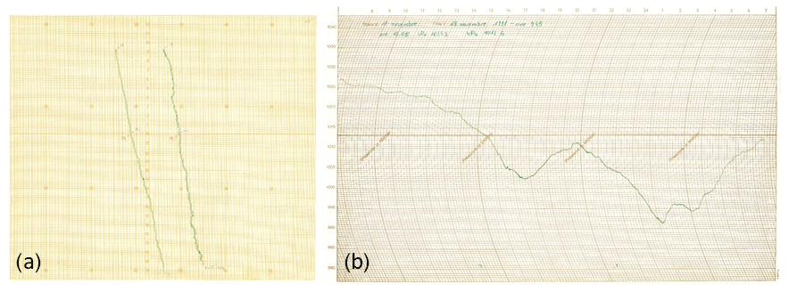
Figure 2(a) Sprung-Fuess barograph chart from 2 February 1954 at 10:00 to 4 February 1954 at 09:00. (b) Fuess 87M barograph chart from 11 November 1991 at 10:05 to 18 November 1991 at 09:45.

Figure 3Daily corrections (c, panel a) and errors (σ, panel b) from 1841 to 1920 in hectopascals. From 1920 onwards, c=0 hPa and σ=0.06 hPa.
The environmental error is caused by pressure fluctuations occurring at sub-hourly timescales that may affect the (nominally) instantaneous measurement.
No information was found about errors on the instrumental corrections. With regard to the normalization to a standard barometer, errors were only found for the Kappeller N. 17, 1004, and 710 barometers, namely 0.16, 0.15, and 0.12 hPa, respectively (Central-Anstalt, 1866, 1869, 1870). We assume that a typical normalization error of 0.10–0.15 hPa can be acceptable for the control barometers.
Mercury barometers were provided with verniers, and the nominal reading precisions were 0.1 mm (0.133 hPa) for the Kappeller N. 1004 and 710 barometers (Polli, 1951–1952), and 0.05 mm (0.067 hPa) for the Wild-Fuess N. 462 (Mazelle, 1907; Polli, 1951–1952). The nominal reading precision of barographs can be estimated as half the interval between the chart markings, namely 0.1 mm (0.133 hPa) for the Sprung-Fuess barograph (Fig. 2a) and 0.25 hPa for the Fuess 85M (Fig. 2b). The accuracy of digital instruments is about 0.2 hPa.
The environmental error was estimated as the average hourly pressure range. These were computed using the hourly pressure extremes, available for 2008–2017. The mean hourly pressure range turns out to be 0.13 hPa, and on 90 % of the days it is lower than 0.24 hPa.
Thus, taking all errors into account, we cautiously assumed the observational error on an individual reading (σo) to be 0.3 hPa, independent of time. The errors on the climatological values, σc and σ24c, were obtained as the standard deviations of Pc and P24c, respectively (Eqs. 1 and 2), to account for the interannual variability of pressure. For both climatologies (1878–1902 and 1903–1919), σc varies approximately between 4.0 hPa in July and 9.5 hPa in January, while σ24c varies between 0.8 and 2.0 hPa in the same months. These errors are much greater than σo, but they only contribute when the hourly observation is missing.
Figure 3 shows the daily corrections (c, panel a), to be added to the provisional daily means to adjust them to 24 h means, and the related errors (σ, panel b). Only the 1841–1920 period is displayed because, from February 1920 onwards, 24 observations per day are always available; therefore c=0 hPa and .06 hPa. Two data sampling schemes can be distinguished, namely in 1841–1867 and 1871–1877, when pressure was observed three times per day, and in 1868–1870 and from 1878 onwards, when barograph records were available.
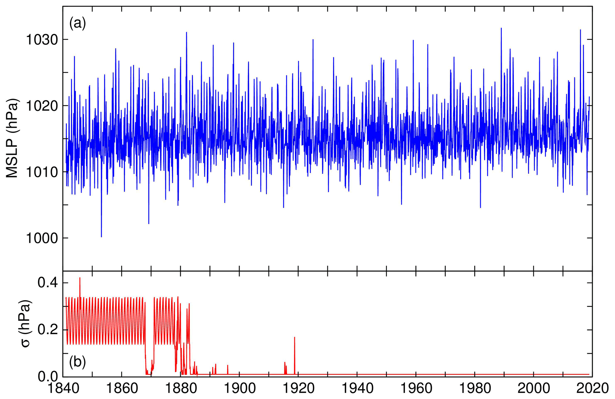
Figure 4Monthly mean-sea-level pressure (MSLP, panel a) and errors (σ, panel b) in hectopascals.
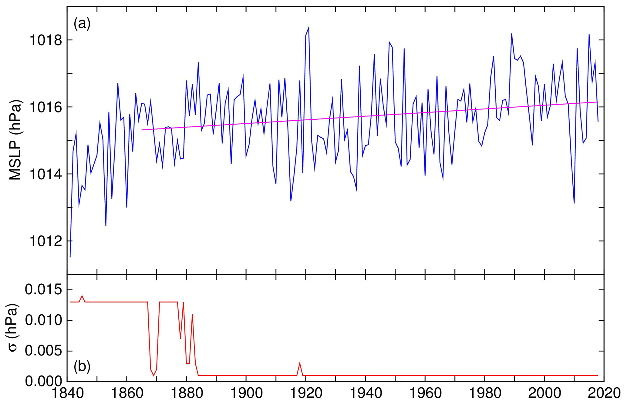
Figure 5Annual mean-sea-level pressure (MSLP, panel a) and errors (σ, panel b) in hectopascals. The 1865–2018 linear trend of 0.5 ± 0.2 hPa per century is shown (magenta line).
When three daily observations are available (1841–1867 and 1871–1877), marked annual cycles of both corrections and errors can be seen due to the seasonal variations of the daily cycle. In 1841–1867, corrections normally range between −0.09 and +0.09 hPa with a mean value of −0.01 hPa, while in 1871–1877, the mean correction is +0.03 hPa, ranging between −0.05 and +0.12 hPa. The difference is the result of changing the time of the evening observation from 22:00 to 21:00. Note that observing at 07:00, 14:00, and 22:00 makes the mean annual bias almost negligible. The spike corresponds to 19 March 1862, when only one observation is available. In 1841–1867, the mean error is 1.30 hPa, and it normally ranges between 0.76 and 1.85 hPa. On solstices and equinoxes of 1843–1864, the error drops to 0.4 hPa. In 1868–1870 and from 1878 onwards, the magnitudes of corrections and errors reflect the abundance of the observations. In the few cases when fewer than three observations are available, .2 hPa and σ attains 1.8 hPa.
The daily means were used to compute monthly (Fig. 4) and annual (Fig. 5) mean pressures and errors. In 1841–1867 and 1871–1877, the monthly error generally varies between 0.15 and 0.35 hPa, and the annual error is less than 0.015 hPa. In 1868–1870 and from 1878 onwards, monthly errors can be as low as 0.01 hPa (Fig. 4b) and annual errors smaller than 0.005 hPa, depending on the number of observations (Fig. 5b).
3.2 Comparison with other stations
In order to detect suspect or erroneous data, we compared the daily means, reduced to 0 ∘C and to MSL, with those of nearby stations, namely the homogenized time series of Padua (1725–1999; Camuffo et al., 2006) and Milan (1763–1998; Maugeri et al., 2002a, b). These time series were selected as they include most of the period of our interest, as only the last 20 years are missing, and because of the relatively short distances from Trieste, namely about 160 and 350 km, respectively. Another reference was used, namely the daily means of mean-sea-level pressure available on a grid from the 20th Century Reanalysis, version 3 (Compo et al., 2011; Giese et al., 2016; Slivinski et al., 2019), interpolated onto the stations' positions. This data set was not used to check the actual pressure values but rather as a help to detect possible persistent anomalies and drifts in the individual local time series.
Note that anomalous pressure differences can temporarily occur between Trieste and Padua or Milan, situated in the Po Plain, that are not related to the barometer performance. Particularly in autumn and winter, the weather in Trieste is often characterized by bora, a katabatic northeasterly wind with mean hourly speeds that can be higher than 20 m s−1 and gusts that can frequently exceed 30 m s−1 (Raicich et al., 2013). Gusty wind causes pressure fluctuations that alter the barometer readings (Liu and Darkow, 1989; WMO, 2018) and, therefore, affect the comparison of daily pressure between Trieste and Padua and/or Milan. Typically, strong bora can last from a couple of days to a week and occasionally up to a couple of weeks (e.g. Raicich et al., 2013).
The daily pressure difference between Trieste and Padua and between Trieste and Milan show anomalous behaviours from 10 March 1844 to 23 May 1846. The 91 d running means, used to smooth day-to-day variability, are displayed in Fig. 6 (only the 1841–1855 period is shown). Seasonal cycles, retained by the running mean, are clearly visible, with higher values in the early months of the year and lower values in the later months. Initially, all the Trieste data reported in the Repertori were reduced to 0 ∘C (Fig. 6, thin lines). However, the amplitudes of the seasonal cycles of the pressure differences appear much larger in March 1844–May 1846. We attributed the anomaly to the fact that, unlike the previous and following observations, the Trieste pressures were written after being reduced to 0 ∘C and, therefore, were erroneously reduced again. Figure 6 (thick curves) shows that the seasonal cycles appear more coherent when the Trieste data from 10 March 1844 to 23 May 1846 are retained as reported in the Repertori.
The anomalous behaviour of the March 1844–May 1846 period was confirmed by comparing the monthly means with those reported in Kreil (1854), Jelinek (1867), Osnaghi (1874), and Mazelle (1889), which were also computed from Gallo's data and explicitly reported to be reduced to 0 ∘C. Perhaps the pressure measured with the Schlosser barometer was reduced for comparison with the data measured with the Hanaczik, mentioned in Sect. 2.2, which were also reduced to 0 ∘C and MSL (Gallo, 1846).
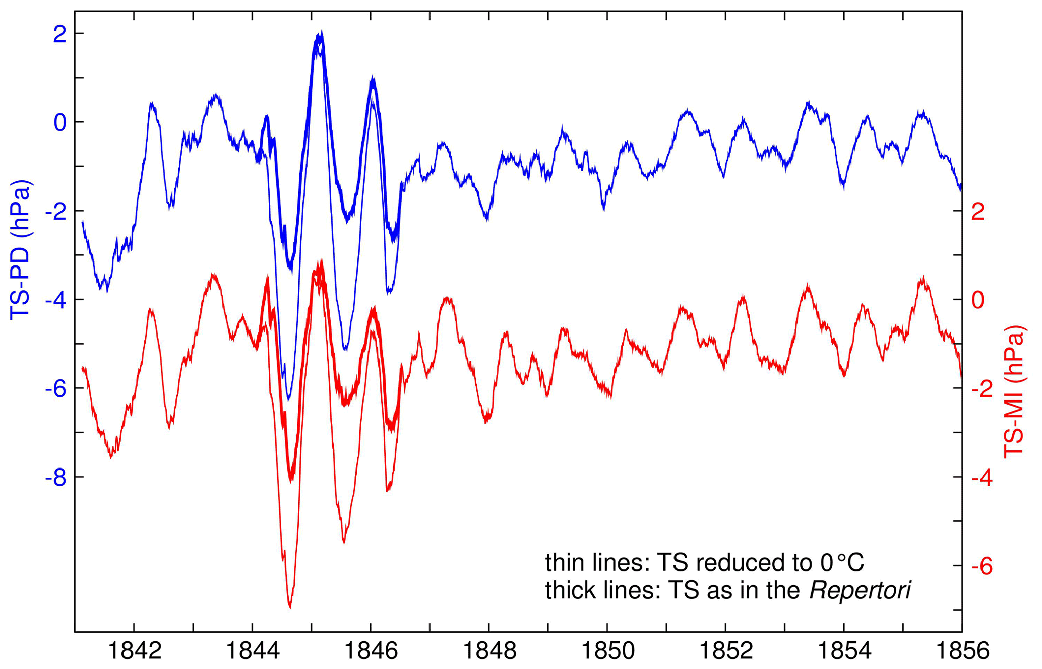
Figure 691 d running means of daily mean-sea-level pressure differences between Trieste (TS) and Padua (PD) (blue curves, left scale) and between Trieste and Milan (MI) (red curves, right scale). The thin lines correspond to Trieste pressure reduced to 0 ∘C, and the thick lines correspond to Trieste pressure from 10 March 1844 to 23 May 1846 as it appears in the Repertori.
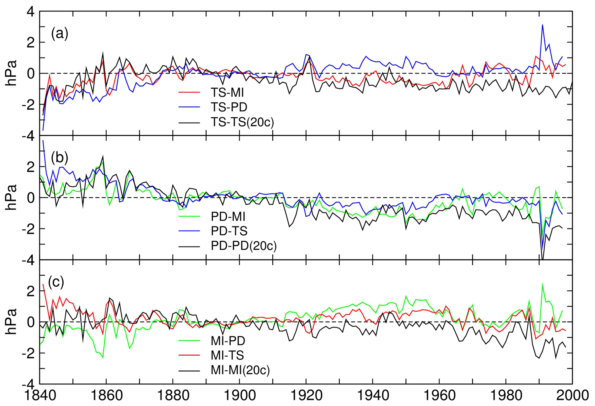
Figure 7Comparisons of annual mean pressures (hPa): (a) differences involving Trieste (TS); (b) differences involving Padua (PD); and (c) differences involving Milan (MI). Black curves represent the comparisons between each station and the corresponding time series from the 20th Century Reanalysis (20c); the comparison between Trieste and Milan is shown in red, that between Trieste and Padua in blue, and that between Padua and Milan in green.
The annual differences between pressure at Trieste, Padua, and Milan are displayed in Fig. 7. In earlier decades, Trieste seems to be lower than expected by at least 1 hPa until the mid-1850s, relative to all the reference time series (Fig. 7a). Another anomaly may occur in the early 1860s but not relative to the reanalysis. The year 1921 also seems anomalous; note that two instrument height changes took place in 1920 (Table 3).
In general, the differences between station data and the respective reanalysis decrease. The average rates from 1861 (after the increase observed at Trieste) onwards are −1.1 hPa per century (Trieste), −1.9 hPa per century (Padua), and −1.2 hPa per century (Milan). This might be related to the reanalysis behaviour in the area of interest; however, for our purpose, it indicates that the Trieste behaviour cannot be attributed to local observations. Another anomaly in the reanalyses is observed in the 1910s, probably connected with a lack of good observations during WWI. Systematic problems are not easy to detect because, when compared to each other, all the time series seem affected by anomalous behaviours. For instance, Padua data seem too high with respect to both Trieste and Milan from 1920 to 1960 (Fig. 7a, c) and in the early 1990s (Fig. 7b). Milan itself seems affected by a systematic decrease in the early 1960s when compared to the reanalysis; Maugeri et al. (2004) pointed out that the Milan station was relocated in 1951 (Fig. 7c).
We can conclude that Trieste pressure of the 1841–1864 period should be considered suspect, while no other major problems can be detected. We recall that in late December 1856 the barometer was moved to a higher position (Table 3), and in April 1865 a new instrument was introduced (Tables 2, 3). Possible reasons of anomalous behaviours of Trieste data are represented by missing instrumental corrections of the Schlosser barometer, used until March 1865, and inaccurate information about instrument heights.
Besides the time series used for the daily data comparisons, monthly time series are available from other stations close to Trieste, namely Zagreb-Grić (Croatia, 1862–2007) and Ljubljana (Slovenia, 1854–2009), both available from the HISTALP database (Auer et al., 2007), and Udine (Italy, 1803–1855; Meteorologisch Jaarboek, 1871). Overall, these time series allow us to corroborate the conclusions drawn from the comparisons with Milan and Padua daily data. In particular, Udine is coherent with Milan and Padua in 1841–1855, thus confirming the anomalous behaviour of Trieste.
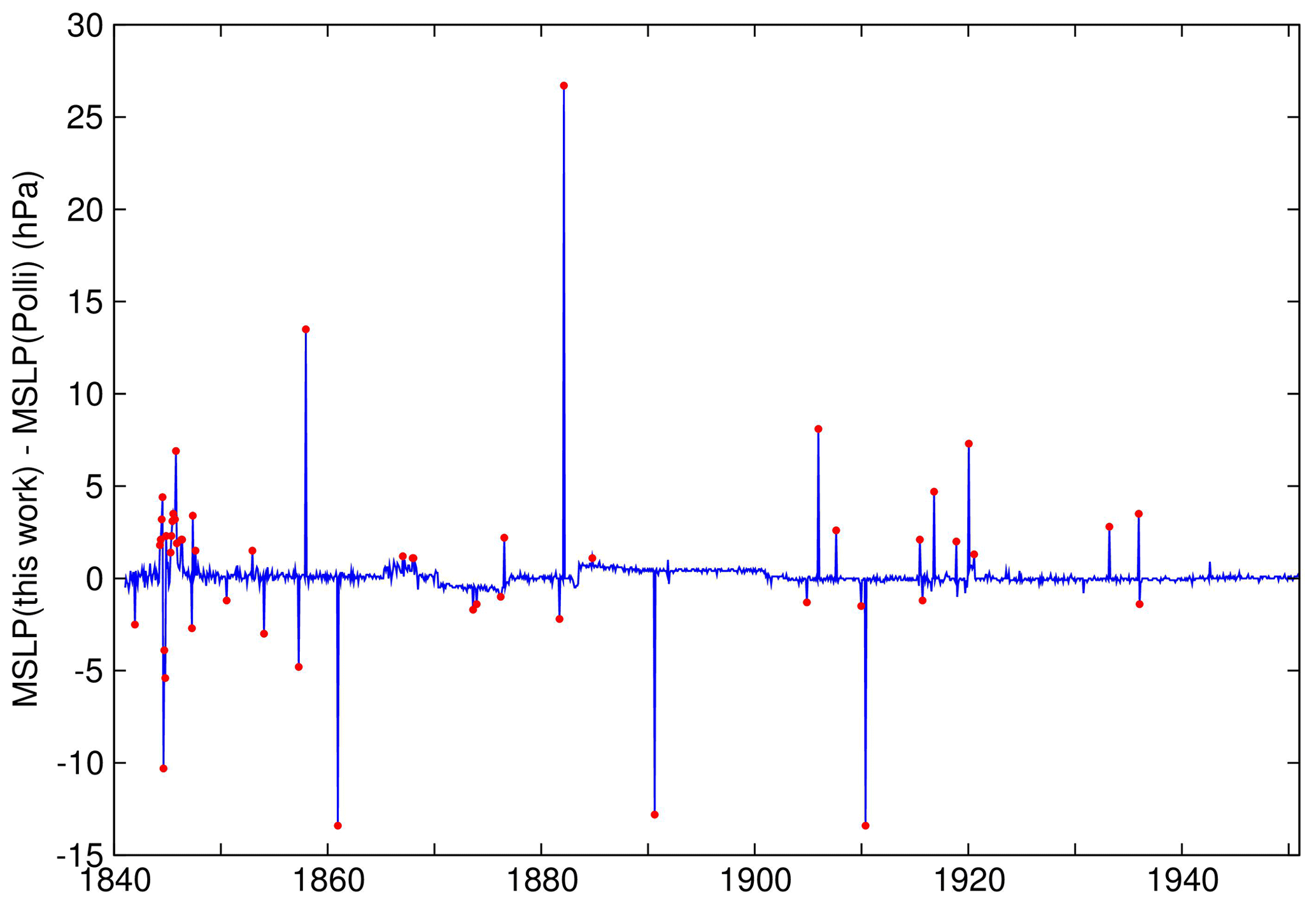
Figure 8Differences between monthly pressures from this work and from Polli (1951–1952). Those exceeding 1 mmHg, i.e. about 1.33 hPa, are highlighted by red dots.
Having discarded the suspect period, Trieste mean-sea-level pressure of 1865–2018 exhibits a trend of 0.5 ± 0.2 hPa per century, significant at p=0.02 (Fig. 5a), after taking into account serial correlation (see details in Appendix B).
3.3 Comparison with previous monthly Trieste time series
A time series of mean daily pressure is discussed in this work for the first time; however, in the past, monthly time series were already produced by different authors (Kreil, 1854; Jelinek, 1867; Osnaghi, 1874; Mazelle, 1889). Much more recently, Polli (1951–1952) summarized the monthly pressures, reduced to the MSL, for 1841–1950.
Figure 8 displays the differences between the monthly means from the present work and those in Polli (1951–1952) that were originally reported in millimetres of mercury (mmHg). The red dots highlight the absolute differences exceeding 1 mmHg, corresponding to about 1.33 hPa, which occur in 53 months out of 1320, i.e. 4 %.
Discrepancies up to a few tenths of a millimetre of mercury are found in most cases, generally due to small differences in calculations or rounding. The data from March 1844 to May 1846 obviously differ as a consequence of the corrections discussed in Sect. 3.2. The step-like discontinuities in 1865, 1868, 1876, and 1903 correspond to changes of the barometer height (Table 3) and are related to the reduction to the MSL. In fact, for each height, average annual corrections were used until 1902 and constant monthly corrections from 1903 onwards. By contrast, we reduced the individual pressure values before further calculations. In at least four cases, pressure was too high or too low by exactly 10 or 20 mmHg due to misprints. In several cases, Polli's data and those in the original data source do not match. Finally, some mistakes may have occurred in the original calculations.
The 1841–2018 daily mean pressures and the derived monthly and annual mean pressure used in this work are available from PANGAEA as “Mean-sea-level atmospheric pressure from 1841 to 2018 at Trieste, Italy” (https://doi.org/10.1594/PANGAEA.926896; Raicich and Colucci, 2021).
Thanks to the observations performed during 178 years, we built a time series of daily mean atmospheric pressures, reduced to 0 ∘C and MSL. Data corrections were generally possible thanks to the metadata reported in the original data sources and in contemporary literature. The daily means were computed from 24 hourly values, when possible, or from the available data amount with adjustments based on climatological values. Errors on the daily means were also estimated, which account for the uncertainties on the instruments performances, known from the metadata, and the uncertainties associated with the adjustment to the 24 h mean, when required. Although the uncertainties on the individual observations can be rather large, even in the early decades the daily errors are always less than 2 hPa, the monthly errors less than 0.4 hPa, and the annual errors less than 0.015 hPa.
A linear trend of 0.5 ± 0.2 hPa per century was estimated for the 1865–2018 period. For comparison with Padua and Milan, the trends were computed over the common period 1865–1997, obtaining highly consistent values, namely 0.48 ± 0.25 hPa per century (Trieste), 0.40 ± 0.24 hPa per century (Padua), and 0.52 ± 0.24 hPa per century (Milan).
In conclusion, the whole data set represents a valuable tool to study the pressure variability particularly on monthly timescales and longer.
We summarize here the main corrections applied to reduce pressure measurements to standard conditions, focussing on the instruments used at Trieste. Jelinek (1876) provided descriptions and discussions of instrument types and methodologies adopted in the 19th century in Austria, while more general information can be found in Abbe (1888) and WMO (2018).
A1 Gravity
The mercury barometer readings were reduced to the standard gravity of 9.80665 m s−2 (WMO, 2018). This is achieved using the relationship
where pg is pressure reduced to standard gravity, p is the observed pressure, gloc is local gravity acceleration, and gstd is standard gravity acceleration. The value gloc=9.80568052 m s−2 was obtained in autumn 1991 in the village of Basovizza, about 8 km east of Trieste (Zerbini et al., 1996); as a result, pg=0.9999 p, and the correction turns out to be negligible. In the past, gravity correction has been disregarded too because the latitude of Trieste, namely 45.75∘ N, is very close to 45∘ N, to which standard gravity used to refer.
A2 Temperature
The barometer readings are affected by the dilatation of the mercury column and of the scale, usually made of brass, caused by temperature variations. The reduction to the standard temperature of 0 ∘C was computed as
where p0 is pressure reduced to 0 ∘C, p is the observed pressure, ∘C−1 and ∘C−1 are the thermal dilatation coefficients of mercury and brass, respectively, and t is the barometer temperature (∘C).
In principle, the Kreil float barograph (Table 2) required a temperature correction that is unknown, but, in practice, its records were normalized to the direct observations. The Sprung-Fuess barograph was temperature-compensated (Mazelle, 1907), as well as the aneroid instruments (Table 2).
A3 Barometer corrections
Fixed-cistern barometers require an adjustment to account for the relative change of mercury heights in the tube and in the cistern. Each Kappeller-type instrument used in Trieste was provided with a factory correction (f), to be added to the measured value, of the form
where c is a constant, specific of the individual instrument, pn is a “neutral” pressure value, and p the observed pressure. By contrast, in the Fortin-type barometers the adjustment to a fixed reference level (zero point) is made by means of a screw; therefore, no such correction is needed. Technical details about the various barometer types used in the 19th century can be found in contemporary literature, for instance Jelinek (1876) and Abbe (1888), as well as in modern articles (e.g. Camuffo et al., 2006; Brugnara et al., 2015).
Another correction is a constant to be added to normalize the measurement to that of a primary barometer. Before 1919, the reference was the Normal Barometer of the Central Institute for Meteorology and Earth Magnetism in Vienna. By contrast, the primary barometer adopted afterwards is unknown.
Capillarity also alters the reading of a mercury barometer. No specific information was found, and we can only assume that its effect was either already included in the known barometer corrections or it was negligible.
Table A1 summarizes the values of the barometer and normalization constants that could be found in the literature and in the original documents (Gallo, 1841–1868; Central-Anstalt, 1856, 1866, 1869, 1870, 1874, 1885; Jelinek, 1867; Adria Commission, 1869; Mazelle, 1889). On the basis of the available information, we corrected the 1841–1868 data. The data for 1868–1902 were already corrected by the observers, but we recomputed the corrections. The data from 1903 onwards were corrected by the observers (Sect. 2.2).
Table A1Mercury barometer corrections and constants of normalization to standard barometers.
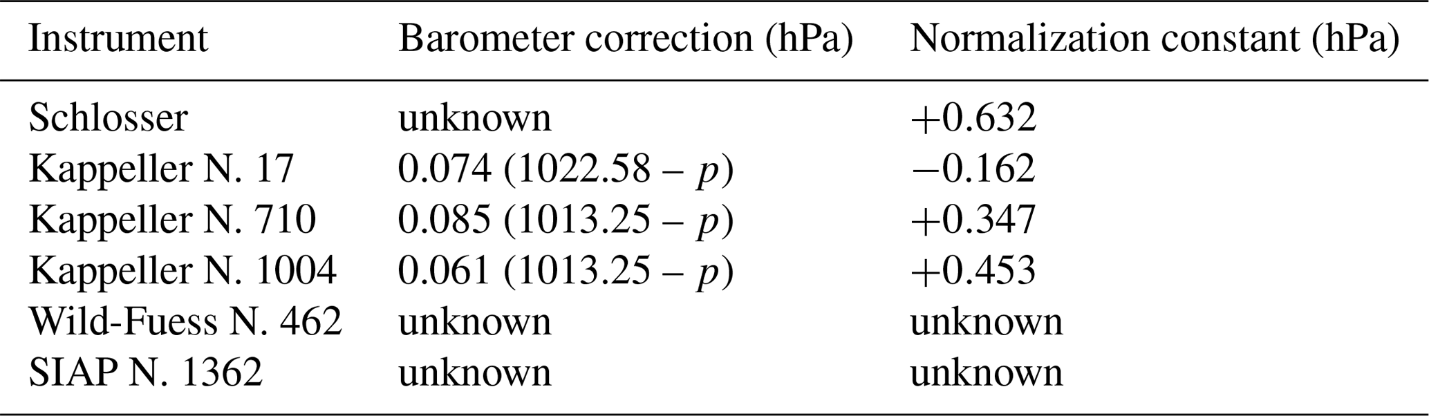
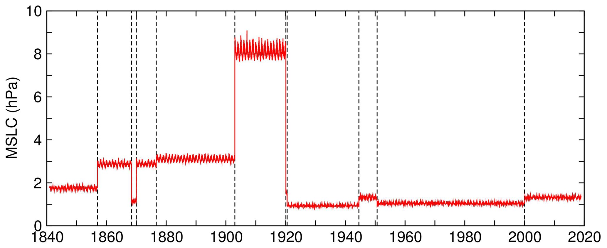
Figure A1Daily corrections to reduce pressure to MSL (MSLC) in hectopascals. The dashed vertical lines correspond to the barometer height changes summarized in Table 3.
A4 Reduction to MSL
The equation used to reduce the station pressure to MSL is
where p0 is the reduced pressure, ps is the station pressure, g is the gravity acceleration, z is the barometer height above MSL, R=287.053 J kg−1 K−1 is the dry air constant, and is the adjusted virtual temperature in kelvin. The formula was taken from Stravisi (1988), which includes the details on the involved variables and the calculation, based on Eq. (16) in WMO (1968), having rewritten some variables. is computed using the observed air temperature and a monthly climatological relative humidity. The adoption of climatological values is justified because the effect of humidity variations on pressure reduction is much smaller than the effect of temperature variations (e.g. WMO, 1954). Figure A1 displays the daily time series of the reductions to MSL, as a function of the barometer heights of Table 3. The seasonal cycle of air temperature causes the high-frequency oscillations.
We estimated the linear trend of the atmospheric pressure time series by linear regression. In order to properly estimate the associated error, the data autocorrelation in time was taken into account. The effect of time autocorrelation is essentially a lower number of degrees of freedom and, if neglected, the consequent underestimation of the standard error.
To account for autocorrelation, we followed Zervas (2001). A time series consisting of n data points is modelled according to
where yk is the detrended mean annual pressure (k runs from 1 to n), obtained by subtracting the linear trend from the original data, b is the slope of the fitting line, tk represents time in years, ρ1 is the lag-1 autoregressive coefficient, and εk is the residual. As a result of autocorrelation, the standard error of the trend increases from σb to (autoregressive) by an amount that can be approximated by the square root of the variance inflation factor (VIF):
where
(Maul and Martin, 1993; von Storch and Zwiers, 2001; Wilks, 2006).
FR retrieved the archived data, prepared the data sets, and led the writing of the paper. RRC was involved in pressure measurement, data collection, and data processing and collaborated in the writing of the paper.
The authors declare that they have no conflict of interest.
Publisher's note: Copernicus Publications remains neutral with regard to jurisdictional claims in published maps and institutional affiliations.
The 20th Century Reanalysis V3 data were provided by the NOAA/OAR/ESRL PSL, Boulder, Colorado, USA, from their website at https://psl.noaa.gov/ (last access: 25 September 2020).
The authors acknowledge the work done by the previous staff of the Commercial and Nautical Academy, the Maritime Observatory, the Astronomical-Meteorological Observatory, the Geophysical Institute, the Thalassographic Institute, and the Institute of Marine Sciences, who managed and performed the observations and processed and preserved the data used to build the data set. In particular, the authors would like to thank Francesco Antonio Immediato, Massimo Iorio, and Emilio Caterini, in the current staff of the Institute of Marine Sciences of CNR.
The authors thank Philip Jones and an anonymous reviewer for their comments that improved the paper.
This paper was edited by Qingxiang Li and reviewed by Philip Jones and one anonymous referee.
Abbe, C.: Treatise on Meteorological Apparatus and Methods, Annual Report of the Chief Signal Officer for 1887, Appendix 46, Government Printing Office, Washington, DC, USA, available at: https://books.google.it/books?id=i0c5AQAAMAAJ&print sec=frontcover&dq=abbe+Treatise+on+Meteorological+Appara tus+and+Methods&hl=it&sa=X&ved=2ahUKEwjv7Mvtqt7rAh XCrIsKHQkYCTwQ6AEwAHoECAUQAg#v=onepage&q=abb e%20Treatise%20on%20Meteorological%20Apparatus%20and %20Methods&f=false (last access: 27 January 2021), 1888.
Adria Commission: Erster Bericht der ständigen Commission für die Adria an die kais, Akademie der Wissenschaften, k.k. Hof- und Staatsdruckerei, Vienna, Austria, available at: https://books.google.it/books?id=8_-ZG6mCcp0C&printsec=frontcover&source=gbs_atb&redir_esc=y#v=onepage&q&f=false (last access: 27 January 2021), 1869.
Auer, I., Böhm, R., Jurkovic, A., Lipa, W., Orlik, A., Potzmann, R., Schöner, W., Ungersböck, M., Matulla, C., Briffa, K., Jones, P., Efthymiadis, D., Brunetti, M., Nanni, T., Maugeri, M., Mercalli, L., Mestre, O., Moisselin, J.-M., Begert, M., Müller-Westermeier, G., Kveton, V., Bochnicek, O., Stastny, P., Lapin, M., Szalai, S., Szentimrey, T., Cegnar, T., Dolinar, M., Gajic-Capka, M., Zaninovic, K., Majstorovic, Z., and Nieplova, E.: HISTALP – Historical instrumental climatological surface time series of the greater Alpine region, Int. J. Climatol., 27, 17–46, https://doi.org/10.1002/joc.1377, 2007.
Brönnimann, S., Allan, R., Ashcroft, L., Baer, S., Barriendos, M., Brázdil, R., Brugnara, Y., Brunet, M., Brunetti, M., Chimani, B., Cornes, R., Domínguez-Castro, F., Filipiak, J., Founda, D., García Herrera, R., Gergis, J., Grab, S., Hannak, L., Huhtamaa, H., Jacobsen, K. S., Jones, P., Jourdain, S., Kiss, A., Lin, K. E., Lorrey, A., Lundstad, E., Luterbacher, J., Mauelshagen, F., Maugeri, M., Maughan, N., Moberg, A., Neukom, R., Nicholson, S., Noone, S., Nordli, Ø., Ólafsdóttir, K. B., Pearce, P. R., Pfister, L., Pribyl, K., Przybylak, R., Pudmenzky, C., Rasol, D., Reichenbach, D., Řezníčková, L., Rodrigo, F. S., Rohr, C., Skrynyk, O., Slonosky, V., Thorne, P., Valente, M. A., Vaquero, J. M., Westcott, N. E., Williamson, F., and Wyszyński, P.: Unlocking pre-1850 instrumental meteorological records. A Global Inventory, B. Am. Meteorol. Soc., 100, ES389–ES413, https://doi.org/10.1175/BAMS-D-19-0040.1, 2019.
Brugnara, Y., Auchmann, R., Brönnimann, S., Allan, R. J., Auer, I., Barriendos, M., Bergström, H., Bhend, J., Brázdil, R., Compo, G. P., Cornes, R. C., Dominguez-Castro, F., van Engelen, A. F. V., Filipiak, J., Holopainen, J., Jourdain, S., Kunz, M., Luterbacher, J., Maugeri, M., Mercalli, L., Moberg, A., Mock, C. J., Pichard, G., Řezníčková, L., van der Schrier, G., Slonosky, V., Ustrnul, Z., Valente, M. A., Wypych, A., and Yin, X.: A collection of sub-daily pressure and temperature observations for the early instrumental period with a focus on the “year without a summer” 1816, Clim. Past, 11, 1027–1047, https://doi.org/10.5194/cp-11-1027-2015, 2015.
Camuffo, D. and Jones, P.: Improved Understanding of Past Climatic Variability from Early Daily European Instrumental Sources, Kluwer Academic Publishers, Dordrecht, The Netherlands, 2002.
Camuffo, D., Cocheo, C., and Sturaro, G.: Corrections of systematic errors, data homogenisation and climatic analysis of the Padova pressure series (1725–1999), Climatic Change, 78, 493–514, https://doi.org/10.1007/s10584-006-9052-3, 2006.
Central-Anstalt: Jahrbücher der k.k. Central-Anstalt für Meteorologie und Erdmagnetismus, Jahrgang 1852, IV Band, k.k. Hof- und Staatsdruckerei, Vienna, Austria, available at: https://opacplus.bsb-muenchen.de/title/BV042125944 (last access: 27 January 2021), 1856.
Central-Anstalt: Jahrbücher der k.k. Central-Anstalt für Meteorologie und Erdmagnetismus, Jahrgang 1864, N.F. I Band, k.k. Hof- und Staatsdruckerei, Vienna, Austria, available at: https://opacplus.bsb-muenchen.de/title/BV042125944 (last access: 27 January 2021), 1866.
Central-Anstalt: Jahrbücher der k.k. Central-Anstalt für Meteorologie und Erdmagnetismus, Jahrgang 1867, N.F. IV Band, k.k. Hof- und Universitäts-Buchhändler, Vienna, Austria, available at: https://opacplus.bsb-muenchen.de/title/BV042125944 (last access: 27 January 2021), 1869.
Central-Anstalt: Jahrbücher der k.k. Central-Anstalt für Meteorologie und Erdmagnetismus, Jahrgang 1868, N.F. V Band, k.k. Hof- und Universitäts-Buchhändler, Vienna, Austria, available at: https://opacplus.bsb-muenchen.de/title/BV042125944 (last access: 27 January 2021), 1870.
Central-Anstalt: Jahrbücher der k.k. Central-Anstalt für Meteorologie und Erdmagnetismus, Jahrgang 1872, N.F. IX Band, k.k. Hof- und Universitäts-Buchhändler, Vienna, Austria, available at: https://opacplus.bsb-muenchen.de/title/BV042125944 (last access: 27 January 2021), 1874.
Central-Anstalt: Jahrbücher der k.k. Central-Anstalt für Meteorologie und Erdmagnetismus, Jahrgang 1882, N.F. XIX Band, k.k. Hof- und Universitäts-Buchhändler, Vienna, Austria, available at: https://opacplus.bsb-muenchen.de/title/BV042125944 (last access: 27 January 2021), 1884.
Central-Anstalt: Jahrbücher der k.k. Central-Anstalt für Meteorologie und Erdmagnetismus, Jahrgang 1884, N.F. XXI Band, k.k. Hof- und Universitäts-Buchhändler, Vienna, Austria, available at: https://opacplus.bsb-muenchen.de/title/BV042125944 (last access: 27 January 2021), 1885.
Cocheo, C. and Camuffo, D.: Corrections of systematic errors and data homogenisation in the daily temperature Padova time series (1725–1998), Climatic Change, 53, 77–100, https://doi.org/10.1023/A:1014950306015, 2002.
Compo, G. P., Whitaker, J. S., Sardeshmukh, P. D., Matsui, N., Allan, R. J., Yin, X., Gleason, B. E., Vose, R. S., Rutledge, G., Bessemoulin, P., Brönnimann, S., Brunet, M., Crouthamel, R. I., Grant, A. N., Groisman, P. Y., Jones, P. D., Kruk, M., Kruger, A. C., Marshall, G. J., Maugeri, M., Mok, H. Y., Nordli, Ø., Ross, T. F., Trigo, R. M., Wang, X. L., Woodruff, S. D., and Worley, S. J.: The Twentieth Century Reanalysis Project, Q. J. Roy. Meteor. Soc., 137, 1–28, https://doi.org/10.1002/qj.776, 2011.
Cornes, R. C., Jones, P. D., Briffa, K. R., and Osborn, T. J.: A daily series of mean sea-level pressure for London, 1692–2007, Int. J. Climatol., 32, 641–656, https://doi.org/10.1002/joc.2301, 2012a.
Cornes, R. C., Jones, P. D., Briffa, K. R., and Osborn, T. J.: A daily series of mean sea-level pressure for Paris, 1670–2007, Int. J. Climatol., 32, 1135–1150, https://doi.org/10.1002/joc.2349, 2012b.
Gallo, V.: Repertori, 7 volumes, CNR-ISMAR Archive, Trieste, Italy, 1841–1868.
Gallo, V.: Sullo stato attuale della meteorologia in Trieste, in: C. Palomba e Comp., Raccolta di lettere ed altri scritti attorno alla fisica e alle matematiche, Anno II, 54–57, 114–117, 147–148, 194–196, 212–213, 289–295, 323–325, Tip. Marini e Morini, Rome, Italy, available at: https://books.google.it/books?id=YTU3AAAAYAAJ&printsec= frontcover&dq=Raccolta+di+lettere+ed+altri+scritti+attorno+ alla+fisica+e+alle+matematiche&hl=it&sa=X&ved=2ahUKEwiK 5ZroqN7rAhViposKHcY8B5YQ6AEwAHoECAEQAg#v= onepage&q=Raccolta di lettere ed altri scritti attorno alla fisica e alle matema40&f=false (last access: 27 January 2021), 1846.
Giese, B. S., Seidel, H. F., Compo, G. P., and Sardeshmukh, P. D.: An ensemble of ocean reanalyses for 1815–2013 with sparse observational input, J. Geophys. Res.-Oceans, 121, 6891–6910, https://doi.org/10.1002/2016JC012079, 2016.
I.R. Accademia di Commercio e Nautica: Prospetto degli studj dell'I.R. Accademia di Commercio e Nautica per l'anno scolastico 1852–1853, Tipografia del Governo, Trieste, 38 pp., 1853.
Jelinek, C.: Anleitung zur Anstellung meteorologischer Beobachtungen und Sammlung von Hilfstafeln, k.k Hof- und Staatsdruckerei, Vienna, Austria, available at: https://books.google.it/books/about/Anleitung_zur_Anstellung_meteorologische.html?id=Yt9Lo9e2914C&redir_esc=y (last access: 27 January 2021), 1876.
Jelinek, K.: Über den Jährlichen Gang der Temperatur und Luftdruckes in Österreich und an einigen benachbarten Stationen. k.k. Akademie der Wissenschaften, Denkschriften der mathematisch-naturwissenschaftlichen Classes, XXVI Band, 28–63, available at: https://books.google.it/books?id=a29FAQAAMAAJ&pg=PA1&dq= Jelinek,+K.:+%C3%9Cber+den+J%C3%A4hrlichen+Gang+der+ Temperatur+1867&hl=it&sa=X&ved=2ahUKEwi9puCkqN7rAh VmoosKHWtGDxQQ6AEwAnoECAYQAg#v=onepage&q&f= false (last access: 27 January 2021), 1867.
Kreil, K. (Ed.): Mehrjärige Beobachtungen in Triest, Vom Jahre 1841 bis 1850, Jahrbücher der k.k. Central-Anstalt von Meteorologie und Erdmagnetismus, I. Band – Jahrgang 1848 und 1849, k.k. Hof- und Staatsdruckerei, Wien, 196–207, 1854.
Liu, H. and Darkow, G.: Wind effect on measured atmospheric pressure, J. Atmos. Ocean. Tech., 6, 5–12, https://doi.org/10.1175/1520-0426(1989)006<0005:WEOMAP>2.0.CO;2, 1989.
Martini, A.: Manuale di Metrologia, Ossia Misure, Pesi e Monete in Uso Attualmente e Anticamente Presso Tutti i Popoli, Loescher, Turin, Italy, available at: http://www.braidense.it/dire/martini/indice.htm (last access: 27 January 2021), 1883.
Maugeri, M., Buffoni, L., and Chlistovsky, F.: Daily Milan temperature and pressure series (1763–1998): history of the observations and data and metadata recovery, Climatic Change, 53, 101–117, https://doi.org/10.1023/A:1014970825579, 2002a.
Maugeri, M., Buffoni, L., Delmonte, B., and Fassina, A.: Daily Milan temperature and pressure series (1763–1998): Completing and homogenising the data, Climatic Change, 53, 119–149, https://doi.org/10.1023/A:1014923027396, 2002b.
Maugeri, M., Brunetti, M., Monti, F., and Nanni, T.: Sea-level pressure variability in the Po Plain (1765–2000) from homogenized daily secular records, Int. J. Climatol., 24, 437–455, https://doi.org/10.1002/joc.991, 2004.
Maul, G. A. and Martin, D. M.: Sea Level rise at Key West, Florida, 1846–1992: America's longest instrumental record?, Geophys. Res. Lett., 20, 1955–1958, https://doi.org/10.1029/93GL02371, 1993.
Mazelle, E.: Ueber den Luftdruck in Triest, Rapporto annuale dell'Osservatorio Marittimo 1886, Tipografia del Lloyd Austro-ungarico, Trieste, Italy, 1889.
Mazelle, E.: Prefazione, Rapporto annuale dell'Osservatorio Marittimo 1903, Tipografia del Lloyd Austriaco, Trieste, Italy, 1907.
Meeus, J.: Astronomical algorithms, Willmann-Bell Inc., Richmond, VA, USA, 1998.
Meteorologisch Jaarboek: Meteorologisch Jaarboek voor 1870, Koninklijk Nederlandsch Meteorologisch Instituut, Utrecht, The Netherlands, available at: https://opacplus.bsb-muenchen.de/Vta2/bsb11035259/bsb:43925481871 (last access: 2 June 2021), 1871.
Osnaghi, F.: Zusammenstellung der Monat- und Jahresmittel sowie der Extreme aus den meteorologischen Beobachtungen der k.k. Handels- und nautischen Akademie in Triest für die Jahre 1841–1873, Jahrbücher der k.k. Central-Anstalt von Meteorologie und Erdmagnetismus, neue Folge IX. Band – Jahrgang 1872, k.k. Hof- und Staatsdruckerei, Vienna, Austria, 173–195, available at: https://opacplus.bsb-muenchen.de/title/BV042125944 (last access: 27 January 2021), 1874.
Osnaghi, F.: Prefazione, Rapporto annuale dell'Osservatorio Marittimo 1884, Tipografia del Lloyd Austro-ungarico, Trieste, Italy, 1886.
Polli, S.: 110 anni di osservazioni meteoriche eseguite a Trieste (1841–1950), P. VII. Le serie barometriche, Boll. Soc. Adr. Sc. Nat., 46, 111–122, 1951–1952.
Raicich, F. and Colucci, R. R.: A near-surface sea temperature time series from Trieste, northern Adriatic Sea (1899–2015), Earth Syst. Sci. Data, 11, 761–768, https://doi.org/10.5194/essd-11-761-2019, 2019.
Raicich, F. and Colucci, R. R.: Mean-sea-level atmospheric pressure from 1841 to 2018 at Trieste, Italy, PANGAEA, https://doi.org/10.1594/PANGAEA.926896, 2021.
Raicich, F., Malačič, V., Celio, M., Giaiotti, D., Cantoni, C., Colucci, R.R., Čermelj, B., and Pucillo, A.: Extreme air-sea interactions in the Gulf of Trieste (North Adriatic) during the strong Bora event in winter 2012, J. Geophys. Res.-Oceans, 118, 5238–5250, https://doi.org/10.1002/jgrc.20398, 2013.
Rossetti, D.: Elementi per la statistica di Trieste e dell'Istria. Parte I, Archeografo Triestino 1 (1st series), 13–34, available at: https://books.google.it/books?id=BEujYkY4F0AC&hl=it&source=gbs_book_other_versions (last access: 27 January 2021), 1829.
Slivinski, L. C., Compo, G. P., Whitaker, J. S., Sardeshmukh, P. D., Giese, B. S., McColl, C., Allan, R., Yin, X., Vose, R., Titchner, H., Kennedy, J., Spencer, L. J., Ashcroft, L., Brönnimann, S., Brunet, M., Camuffo, D., Cornes, R., Cram, T. A., Crouthamel, R., Domínguez-Castro, F., Freeman, J. E., Gergis, J., Hawkins, E., Jones, P. D., Jourdain, S., Kaplan, A., Kubota, H., Le Blancq, F., Lee, T., Lorrey, A., Luterbacher, J., Maugeri, M., Mock, C. J., Moore, G. K., Przybylak, R., Pudmenzky, C., Reason, C., Slonosky, V. C., Smith, C., Tinz, B., Trewin, B., Valente, M. A., Wang, X. L., Wilkinson, C., Wood, K., and Wyszyński, P.: Towards a more reliable historical reanalysis: Improvements for version 3 of the Twentieth Century Reanalysis system, Q. J. Roy. Meteor. Soc., 145, 2876–2908, https://doi.org/10.1002/qj.3598, 2019.
Stravisi, F.: A BASIC program for psychrometric computation and mercury barometer corrections, Università degli Studi di Trieste, Dipartimento di Fisica Teorica, Report FTC 88/3, available at: http://docplayer.net/38480357-A-basic-program-for-psychrometric-computations-and-mercury-barometer-corrections.html (last access: 27 January 2021), 1988.
Stravisi, F.: La meteorologia a Trieste, in: La variabilità del clima locale relazionata ai fenomeni di cambiamento globale, edited by: Cortemiglia, G. C., Pàtron Editore, Bologna, Italy, 245–288, 2006.
von Storch, H. and Zwiers, F. W.: Statistical analysis in climate research, Cambridge University Press, Cambridge, UK, 2001.
Wilks, D. S.: Statistical methods in the atmospheric sciences, Academic Press, Burlington, MA, USA, 2006.
WMO: Reduction of Atmospheric Pressure (Preliminary Report on Problems Involved), WMO Technical Note No. 7, WMO-No. 36.TP.12, Geneva, Switzerland, available at: https://library.wmo.int/doc_num.php?explnum_id=3443 (last access: 27 January 2021), 1954.
WMO: Methods in Use for the Reduction of Atmospheric Pressure, WMO Technical Note No. 91, WMO-No. 226.TP.120, Geneva, Switzerland, available at: https://library.wmo.int/doc_num.php?explnum_id=3445 (last access: 27 January 2021), 1968.
WMO: Guide to Meteorological Instruments and Methods of Observation, Volume I – Measurements of meteorological Variables, WMO-No. 8, Geneva, Switzerland, available at: https://library.wmo.int/doc_num.php?explnum_id=10179 (last access: 27 January 2021), 2018.
Zerbini, S., Plag, H.-P., Baker, T., Becker, M., Billiris, H., Bürki, B., Kahle, H.-G., Marson, I., Pezzoli, L., Richter, B., Romagnoli, C., Sztobryn, M., Tomasi, P., Tsimplis, M., Veis, G., and Verrone, G.: Sea level in the Mediterranean: a first step towards separating crustal movements and absolute sea-level variations, Global Planet. Change, 14, 1–48, https://doi.org/10.1016/0921-8181(96)00003-3, 1996.
Zervas, C. E.: Sea level variations of the United States, 1854–1999, NOAA Technical Report NOS CO-OPS 36, U.S. Dept. of Commerce, National Oceanic and Atmospheric Administration, National Ocean Service, Silver Spring, MD, USA, available at: https://data.globalchange.gov/report/noaa-nos-co-ops-36 (last access: 10 September 2020), 2001.