A national topographic dataset for hydrological modeling over the contiguous United States

Topography is a fundamental input to hydrologic models critical for generating realistic streamflow networks as well as infiltration and groundwater flow. Although there exist several national topographic datasets for the United States, they may not be compatible with gridded models that require hydrologically consistent digital elevation models (DEMs). Here, we present a national topographic dataset developed to support gridded hydrologic simulations at 1 km and 250 m spatial resolution over the contiguous United States. The workflow is described step by step in two parts: (a) DEM processing using a Priority Flood algorithm to ensure hydrologically consistent drainage networks and (b) slope calculation and smoothing to improve drainage performance. The accuracy of the derived stream network is evaluated by comparing the derived drainage area to drainage areas reported by the national stream gage network. The slope smoothing steps are evaluated using the runoff simulations with an integrated hydrologic model. Our DEM product started from the National Water Model DEM to ensure our final datasets will be as consistent as possible with this existing national framework. Our analysis shows that the additional processing we provide improves the consistency of simulated drainage areas and the runoff simulations that simulate gridded overland flow (as opposed to a network routing scheme). The workflow uses an open-source R package, and all output datasets and processing scripts are available and fully documented. All of the output datasets and scripts for processing are published through CyVerse at 250 m and 1 km resolution. The DOI link for the dataset is https://doi.org/10.25739/e1ps-qy48 (Zhang and Condon, 2020).

1 Introduction

Topography is one of the most important inputs to hydrologic simulations; it defines watershed boundaries and shapes river networks. Surface flow travel times and runoff characteristics are very sensitive to hillslope characteristics (D'Odorico and Rigon, 2003; Freer et al., 2002; Frei et al., 2010; Gupta and Mesa, 1988). In addition to shaping surface flow networks, groundwater fluxes and residence times are also strongly driven by topographic gradients (e.g., Condon and Maxwell, 2015). High-resolution elevation data are not difficult to find; for example the National Elevation Dataset provides a 30 m resolution digital elevation model (DEM) across the US (Gesch et al., 2002). It is well established that topographic datasets require processing to be suitable for hydrologic simulation because flow networks and slopes can be sensitive to noise in the DEM and can be affected by the resolution and spatial gridding of a DEM (Habtezion et al., 2016; Sørensen and Seibert, 2007; Thompson et al., 2001; Vaze et al., 2010; Wolock and McCabe, 2000; Wu et al., 2008; Zhang and Montgomery, 1994). This processing generally consists of some combination of steps to (1) remove erroneous local minima that impeded flow (Kenny et al., 2008; Lindsay, 2016a, b); (2) lower or “burn” in the drainage network to ensure that flow occurs along identified stream segments (Lindsay, 2016b; Woodrow et al., 2016), and (3) smooth the DEM to remove noise introduced by the sampling resolution (Gallant, 2011; Lindsay et al., 2019).

Although there are many tools and methods available to process topography for hydrologic applications, processing is generally site specific, and we lack a national topographic dataset for the US that is designed specifically for gridded physical hydrology simulations. At the national scale there are four main topographic datasets for the US. First, as previously noted the National Elevation Dataset (NED), provides 30 m national DEM primarily derived from the U.S. Geological Survey (USGS) 10 and 30 m DEMs (Gesch et al., 2002). This provides a high-resolution national topographic dataset that includes hydrologic information such as flow directions and accumulation; however, it is not directly processed for DEM-based hydrologic simulations which may require more smoothing.

Second, the National Hydrography Dataset Plus (NHDPlus) dataset provides a collection of geospatial data, including various key features of stream network including elevation, drainage area and watershed boundary, in multiple resolutions, i.e., NHDPlus High Resolution in 10 m and NHD Medium Resolution in 30 m. It is derived from the 10 m USGS elevation data and the national complete Watershed Boundary Dataset (Viger et al., 2016). Because of its public availability, high resolution and large spatial coverage, the dataset has been applied in many hydrologic studies considering runoff, river routing and flood inundation (David et al., 2011; Garousi-Nejad et al., 2019; Smith et al., 2013; Zhang et al., 2018). The NHDPlus dataset provides the most complete hydrologic mapping of the US; however, spatial inconsistences and noise in these datasets make it difficult to use these data directly for gridded hydrologic modeling. The NHDPlus stream network is derived from various topographic map sources, leading to spatial inconsistencies and inaccuracies in river network (Moore et al., 2019). Spatial discrepancies have also been found between NHDPlus and the local higher-resolution light detection and ranging data (lidar)-derived stream network (Samu, 2012). It was found that the NHDPlus stream network is not well aligned with DEM-used height above nearest drainage (HAND), which can lead to discrepancies in hydraulic properties for NHDPlus reaches (Garousi-Nejad et al., 2019).

Third, the National Water Model (NWM) is a national hydrologic modeling framework that simulates terrestrial hydrology at 250 m spatial resolution. This model has its own DEM and stream mask that are derived from the 30 m DEM in NED and stream network in NHDPlus (Gochis et al., 2018). The NWM DEM was developed using the TauDEM topographic processing tool (Tarboton, 2005) to generate a connected drainage network (Gochis et al., 2018). Although the NWM DEM does include hydrologically based topographic processing, the NWM configuration that this dataset was assembled for uses a network routing approach for streamflow (as opposed to gridded streamflow simulations directly applied to the DEM) (Gochis et al., 2018; Johnson et al., 2019). As a result, stream gradients are calculated on a reach-by-reach basis using an abstracted stream network rather than resulting directly from the gridded DEM. For hydrologic models that rely on partial differential equations (PDEs) to simulate gridded streamflow, additional smoothing and DEM processing is required to improve simulation performance. These models require a topographic dataset which represents these stream reaches accurately within the DEM itself. Also, in PDE-based simulations fluxes occur across grid cell faces, so improved performance can be achieved by directly aligning the DEM processing with grid cell faces.

Finally, the Hydrological data and maps based on SHuttle Elevation Derivatives at multiple Scales (HydroSHEDS) provide hydrographic information for global-scale applications. It offers a set of hydrological datasets, including river networks, watershed boundaries, drainage directions and flow accumulations at ∼ 90 m resolution based on a high-resolution elevation data from NASA's Shuttle Radar Topography Mission (SRTM) (Wickel et al., 2007). HydroSHEDS does include a hydrologically conditioned DEM derived through a series of processing steps, including stream burning, “weeding” of coastal zones and sink filling, as well as river and flow direction layers similar to NHDPlus (Lehner et al., 2006). Previous studies have compared NHD to HydroSHEDS within the US and have shown that NHD has a more complete drainage network (Guth, 2011). Here we stick with the NHD dataset because it has been developed and more rigorously evaluated for the US specifically, and because it has already been mapped to the USGS stream gage network (David et al., 2011).

Here we present a topographic dataset of the contiguous United States (CONUS) designed for PDE-based hydrologic modeling applications that simulate surface and subsurface flows with a single, consistent topographic input. The workflow is discussed step by step in the following sections in two parts: (a) DEM processing by Priority Flood algorithm and (b) slope calculation and smoothing. Several cases are implemented for both parts with comparative analysis to illustrate the improvements of additional procedures. We compared the drainage area with measurements and applied slope into a hydrologic model to evaluate the surface flow simulation.

2 Data and methods

This section covers the detailed information about input datasets including DEM and stream network maps (Sect. 2.1), topographic processing methodology for DEM adjustment and slope calculation (Sect. 2.2), and evaluation metrics used to assess the accuracy of the drainage network and drainage performance (Sect. 2.3).

2.1 Domain and input datasets

Our approach requires three primary inputs: (1) a gridded DEM of topography, (2) a mask of known stream locations, and (3) a mask of lakes and terminal points for endorheic basins (shown in Fig. 1). All analysis covers CONUS plus areas in Canada and Mexico that drain to CONUS. This spatial coverage is consistent with the NOAA National Water Model (NWM) (Sampson and Gochis, 2018). All analysis is completed and available at 1 km and 250 m spatial resolution, but for the purposes of discussion we focus on the 1 km analysis throughout the results section. Our input datasets are primarily derived from the NWM version 1.2. The NWM inputs are derived from publicly available national datasets and have already been processed for hydrologic consistency within their modeling framework, which provides an ideal starting point for this work.

Note that we intentionally start from NWM datasets as opposed to a raw DEM product in order to ensure that the resulting products are as consistent as possible with this growing framework of national hydrologic datasets. Our processing only adjusts the NWM processing where it is needed to improve performance of gridded simulations. This approach is intended to minimize DEM-based discrepancies between modeling approaches and to facilitate future model comparisons and coupling between different modeling approaches.

We start from a 250 m DEM that was developed for the NWM V1.2, which was developed from the 30 m resolution National Elevation Dataset (Gesch et al., 2002) and processed using the TauDEM (Tarboton, 2005) to ensure drainage in a D8 routing scheme (i.e., with flow allowed out of every grid cell in eight directions). The NED dataset provides elevation of bare ground without considering the tall vegetation. We start from this DEM directly for 250 m analysis, and for the 1 km analysis we upscale the NWM DEM by selecting the minimum elevation within every 1 km cell (Condon and Maxwell, 2019). The derived stream network is significantly affected by the upscaling approach (Moretti and Orlandini, 2018). The DEM is upscaled based on the minimum as opposed to the average because this is appropriate in identifying the lowest points and capturing hydrologic features such as streams.

The stream network mask is derived from a rasterized version of the NWM stream vector subset based on Strahler stream order thresholds (Horton, 1945; Strahler, 1957) (note that here too we start from the NWM network to ensure consistency between our final product and existing frameworks). The stream mask is used to guide the drainage patterns in the DEM for the topographic processing in this study. By experimenting with different stream densities, we found that the stream networks consisting of fifth-order and higher streams provide the best guidance in 1 km resolution processing and a denser network consisting of third-order and above streams is ideal for 250 m resolution processing. Figure 1 shows the fifth-order stream network that was used for the 1 km DEM processing. For both the third- and fifth-order stream masks additional manual adjustments were made to improve the resulting drainage network, which is discussed in more detail in Sect. 3.1.

The final input is a mask of lakes and terminal points for endorheic basins. Our topographic processing ensures that all grid cells in the domain drain to either an ocean cell, internal lake or a terminal point within endorheic basins, referred to as “sinks”. The lakes and sinks presented in our domain mask provide end points for all internally draining (i.e., not draining to the ocean) cells. We selected 13 major lakes from the NWM lake shapefile, which was developed based on NHDPlus. Only the major terminal lakes which are critical for watershed delineation were included in this topographic processing. The extents of these lakes are rasterized as shown in Fig. 1 with the borders treated as outlets, and the interior lake cells are excluded from topographic processing.

For the more arid endorheic basins, such as are commonly found in the Great Basin of the western US, intermittent rivers drain to much smaller water bodies which may not be perennially inundated. For these basins, we designate single cells at the river outlet as sink cells which were added to the domain manually based on the fifth-order stream mask. A total of 262 sinks were added to the domain as shown in Fig. 1. The significance of these sinks for topographic processing is discussed further in Sect. 3.1.

Figure 1 Map of the DEM dataset, stream network, lakes and sinks used for processing the 1 km hydrographic dataset.

2.2 Topographic processing workflow

While some hydrologic processing has already been implemented in NWM DEM as described in the previous section, additional processing is needed for the purpose of our processing (1) to ensure a fully connected drainage network for fluxes occurring across cell faces and (2) to improve runoff performance for gridded overland flow simulations. In our processing, we require drainage be accomplished in D4 (i.e., only in the primary north, south, east, west directions); this is useful for partial differential equation (PDE)-based hydrologic simulations where fluxes occur across cell faces (although it should be noted that each grid cell has both an x and y slope so the resulting vectors can point in any direction). Additionally, we provide additional smoothing and analysis of the resulting river network that is generated within the DEM grid.

Figure 2 summarizes the topographic processing workflow for the final dataset we present. All of the processing steps were completed using the PriorityFlow V1.0 toolbox (Condon and Maxwell, 2019), which is available on GitHub (https://github.com/lecondon/PriorityFlow/releases/tag/v1.0, last access: 5 July 2021) and can be installed as an R library. The parameters for each step of the workflow and their values are provided in Table 1. The primary output from the topographic processing workflow is a hydrologically consistent DEM processed to ensure realistic drainage networks and overland flow patterns. In addition to the DEM, many other outputs are generated throughout the processing that define the drainage network, slopes and watersheds. These outputs are listed in Fig. 2 and summarized in more detail in Sect. 4. The steps of the processing workflow are as follows.

1. Minor stream burning. First we apply a very small stream “burn in”, decreasing the elevation of all cells on the stream mask by 1 m. Stream burning is an approach that has been used in previous studies to enforce flow along predefined channel segments (Lindsay, 2016b). Here a very minor elevation adjustment of 1 m is to help locate streams in very flat parts of the domain where the channel may not be captured at all by the 250 m or 1 km DEM. A larger stream burn is not necessary because the later processing steps ensure that the processed DEM reflects the channel network. We would like to emphasize here that this stream burning step is very small, and it is not intended to control the final stream elevation but just to provide some information on stream location. The subsequent steps are the primary elevation adjustments steps.

2. Initial topographic smoothing. It is well established that the spatial resolution of a DEM can introduce artificial noise in the observed topography. Therefore, before processing we apply a smoothing filter to the DEM (Habtezion et al., 2016). Here we use a feature-preserving smoothing approach from the whitebox library in R to remove the DEM roughness for the domain. The approach is a modified feature-preserving normal vector field smoothing technique, so it is feasible for large DEM raster (Lindsay et al., 2019). To remove the noise as well as preserve the topographic characteristics, the filter kernel size (filter) is set to 20 grid cells, and the maximum difference in normal vectors (norm_diff) is 15^∘. Three elevation-update iterations (num_iter) are implemented with a maximum allowable absolute elevation change (max_diff) of 5 m for the whole domain.

3. Priority Flood algorithm to ensure D4 drainage. To be useful for hydrologic simulation, non-physical local minima must be removed from the domain. In this step, we ensure that every cell in the domain has a drainage path out of the domain or to one of the predefined lake or sink internal boundaries. The Priority Flood algorithm is a well-established and mathematically optimal approach to remove erroneous local minima in a DEM and ensure complete drainage (Barnes et al., 2014; Liu et al., 2009; Soille and Gratin, 1994; Wang and Liu, 2006; Zhou et al., 2016). The standard Priority Flood approach starts from the exit points of a domain and works sequentially inward, lifting cells as required to ensure that every cell is guaranteed a monotonically decreasing path to the exit. The Priority Flood algorithm is mathematically optimal in that it achieves a fully draining DEM with the least possible adjustments (or filling) to the original DEM; however, it may not always yield the desired drainage network given a noisy or low-resolution DEM. To address this limitation, Condon and Maxwell (2019) developed a new approach applying the Priority Flood algorithm in two steps: first along a pre-specified drainage network and then to the rest of the cells in the domain treating the processed stream network as the outlets. In this case we can provide it with the NWM stream network to help ensure that our final solution will be consistent with this framework. With this approach the advantages of the Priority Flood algorithm are maintained by the user and also can incorporate information about the stream network to prioritize drainage along this pre-specified network first. Additionally, the user can specify an optional epsilon height to be added to cells' elevation as they are processed by the algorithm. If an epsilon is used, then filling will be applied such that upstream cells are at least epsilon greater than their downstream neighbor. Here we use a stream_epsilon values of 0 for the first round of processing along the stream and a global_epsilon value of 0.1 m for the rest of the domain. A small value of epsilon is to guarantee the drainage without large change to the original DEM. The results of this processing step are (1) a fully draining DEM and (2) a set of D4 flow directions indicating the primary flow direction for every grid cell in the domain.

4. Stream elevation smoothing. While the Priority Flood algorithm ensures a monotonically decreasing path from any grid cell in the domain to an exit, it does not evaluate the smoothness of this path. Furthermore, at 250 m or 1 km resolution the DEM is more reflective of hillslope scale patterns than channel bathymetry. For physically based hydrologic simulations, slopes along stream channels are an important variable controlling surface water drainage. Smoothing elevation gradients along stream reaches has been shown to decrease artificial ponding and improve the runoff simulations performance (Barnes et al., 2016).

   We first derive a new stream network to be used for the stream elevation smoothing, using a drainage area threshold (stream_th). The flow direction files resulting from the Priority Flood processing can be used to calculate the drainage area for every grid cell in the domain. From this, a stream network of any density can be derived based on the stream_th. This allows us to apply smoothing to a denser stream network than was used in the earlier Priority Flood processing script. The smaller the stream_th is, the denser the identified stream network will be, and the more cells will be smoothed. This stream network can then be divided into segments and associated sub-watersheds. Here we use a drainage area threshold of 100 km².

   Stream segments are smoothed by adjusting the elevations along the segment to maintain a constant slope from the starting to the ending point of each segment. After these adjustments are made to the stream reaches an additional elevation processing pass must be made to ensure that all of the bank cells along a stream reach still drain to the stream. Here we apply an epsilon threshold (bank_epsilon) to require that adjacent cells are at least bank_epsilon greater than their downstream neighbor. The bank adjustment step traverses up a stream segment checking that all cells draining to every stream cell (based on flow direction) are at least bank_epsilon (0.1 m in this dataset) higher. Anywhere this is not the case, neighboring cells are filled accordingly, and processing continues up the bank until it reaches a point where all upstream neighboring cells are fully draining.

5. Slope calculations and final slope smoothing. Some hydrologic simulations require slopes rather than elevations as inputs. Therefore, the final step in processing is to convert the processed DEM to slopes in the x and y directions. Here we include three additional processing steps.

   • a.

     Applying maximum and minimum slope thresholds. Maximum and minimum slope thresholds can be specified globally or for the hillslope (slope_max, slope_min) and stream cells (slope_min_stream) separately. Setting minimum slope thresholds has a similar effect to applying an epsilon in the Priority Flood algorithm; however, it can be preferable because it does not propagate to upstream cells. For example, in very flat portions of the domain, even small epsilons can lead to large DEM adjustments as they are additive. The maximum slope is limited for the whole domain; slope_min and slope_min_stream are set to 10⁻⁴.

   • b.

     Removing or dampening secondary slopes. The priority Flood algorithm provides primary D4 flow directions for every grid cell (referred to as the primary flow direction). However, slopes are calculated for every cell in both x and y directions (i.e., in the primary flow direction and a secondary flow direction). Some previous approaches removed all slopes that transverse to the primary flow direction. For example, if a cell's primary flow direction is north then only its y slope would be used, and its x slope would be set to zero (Barnes et al., 2016). However, previous research has shown that hydrologic performance is improved when secondary slopes are included (Barnes et al., 2014; Daniels et al., 2011). Additional details on slope calculations and secondary slope smoothing can be found in Condon and Maxwell (2019). Here we set no restrictions for the secondary slope outside the stream network but remove the secondary slope along the stream network to improve the drainage inside the stream.

   • c.

     Fixing flat cells. Finally, despite the fact that the Priority Flood algorithm ensures that all cells can drain and there are no local minima in the domain, anomalous water ponding points can still be created where the outlet slope of a grid cell is significantly less than the cells draining to it. Therefore, as a final smoothing step if the total slope out divided by the total slope into a given cell is less than a specified adjustment ratio (adj_th, set to 10⁻³ here), the new outlet slope will be set to initial outlet slope times some scaler (adj_ratio, set to 10 here).

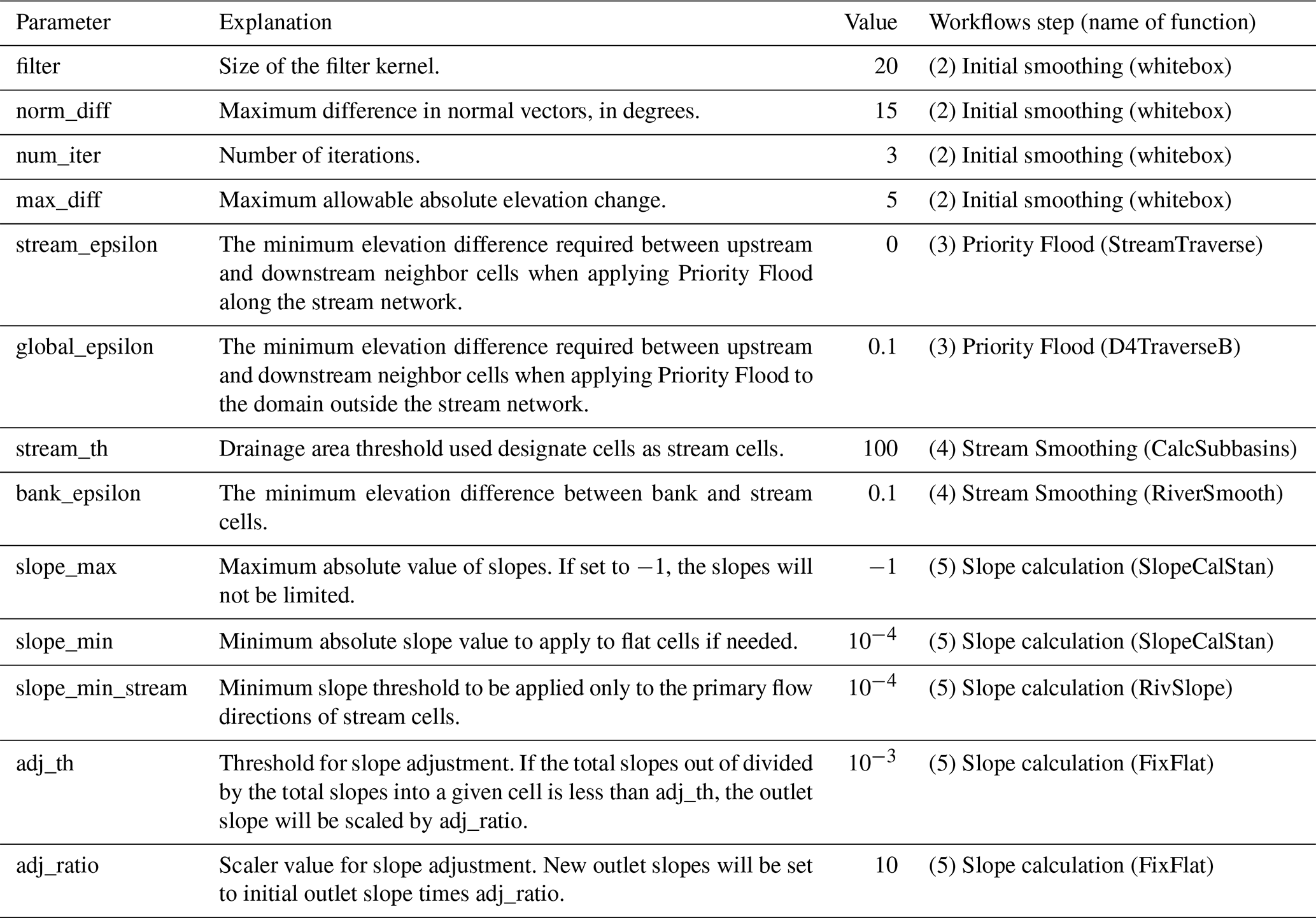
Figure 2 Workflow diagram outlining the major processing steps used and the outputs generated; input parameters are listed in italics and described in more detail in Table 1.

Table 1 Parameters for the topographic processing and values in this dataset.

2.3 Evaluation metrics

As noted in Sect. 2.1, there are already multiple national elevation datasets that are well established and have been previously validated. Our goal is to start from these datasets to develop a national topographic dataset that is as consistent with these products as possible but is designed for gridded overland flow simulation. Because we are starting from established elevation models (DEM for NWM V1.2), our evaluation is focused on the hydrologic improvements to the dataset. Specifically, we evaluate (1) the extent to which the resulting drainage network matches observations and (2) the drainage characteristics of the resulting dataset. Details on the approach for evaluating each of these metrics follow.

1. Accuracy of drainage network. The location of drainage networks can be very sensitive to topographic processing especially when working with relatively-low-resolution DEMs, which do not resolve small stream channels. This is why we incorporate stream network information into the topographic processing with the initial stream burning step and in the Priority Flood algorithm. We evaluate the resulting stream network by calculating the drainage area for every grid cell in the domain based on the derived flow directions and comparing with the drainage areas reported through the USGS stream gage network. The Gages-II dataset includes 7542 gages with drainage area ranging from 0.02 to 2 975 585 km² across the US (Falcone, 2011). When mapping the gages to the DEM we use the reported stream gage latitude and longitude to identify the closest grid cell. We provide a 3 km buffer around each stream gage, allowing the gage to move up to 3 grid cells in any direction for 1 km resolution (12 grid cells for 250 m resolution) if the percentage difference of the resulting drainage area between calculated and USGS observation is less than 20 %. This adjustment step corrects for locations where the grid resolution may result in a gage being mapped to a hillslope cell adjacent to the intended stream cell or where a gage may incorrectly fall on a tributary as opposed the main stem (or vice versa). After allowing for these minor adjustments we evaluate percentage difference in drainage area between the simulated drainage areas based on the topographically processed DEM and the stream gage network.

2. Drainage performance. In addition to the drainage network patterns we apply a hydrologic model to evaluate the hydrologic performance of the entire domain. Here we are concerned primarily with anomalies in the resulting DEM which inaccurately disrupt flow. To test this, we apply the hydrologic model ParFlow (Ashby and Falgout, 1996; Jones and Woodward, 2001; Kollet and Maxwell, 2006; Kuffour et al., 2020; Maxwell, 2013), which is an integrated hydrologic model that includes groundwater and surface water simulation, but for the purposes of this study we focus only on the overland flow simulation. ParFlow simulates overland flow using Manning's equation and the kinematic wave formulation where flow is driven by the bed slope and surface roughness (as specified by Manning's roughness coefficient). Here we evaluate the ponding depth of water over time to evaluate drainage patterns and identify stagnation points.

The model is configured with a single shallow layer (0.1 m) with an impervious surface (permeability in 10⁻⁶ m/h) so that groundwater flow and infiltration processes are essentially ignored. A constant Manning roughness coefficient to 4.4 × 10⁻⁴ is applied across the entire domain. To test the runoff performance, we simulate a single rainfall recession event. The runoff test consists of a 200 h simulation with 1 h rainfall event at a rate of 50 mm followed by 199 h of recession. The intent with this idealized impervious runoff simulation is to isolate the impacts of topography on runoff processes. The runoff test provides an easy visual way to identify locations where the topography is contributing to erroneous runoff behavior and to quantitatively identify locations with poor drainage or anomalous ponding.

3 Topographic processing evaluation

We explored a wide range of parameter combinations in our testing to obtain a reliable topographic dataset for hydrologic modeling. Table 1 outlines all of the parameters that were used for the final topographic processing reflected in the datasets published here. For the purposes of this discussion, we focus on the processing steps that had the largest impact on the accuracy of the resulting drainage network spatially (Sect. 3.1) and the runoff dynamics (Sect. 3.2). The goal here is not to present a sensitivity study of parameters in topographic processing. Rather this discussion is provided to illustrate the key topographic processing steps that can improve hydrologic performance. This section demonstrates the improvements of the published dataset over existing topographic products, specifically for hydrologic modeling applications. Furthermore, the workflow described above and the results presented here can help guide others developing DEMs for different domains or resolutions.

3.1 Drainage network analysis

In this section we explore the impact of incorporating a prior stream network to guide the topographic processing. Figure 3 shows the difference in drainage area between the processed DEM and reported stream gage area when the processing is run without an initial stream mask included in the PriorityFlow adjustment step. Figure 3a shows the percent difference in drainage area for all 7542 gages used for comparison, while Fig. 3b shows only 1195 gages with drainage area over 5000 km². As illustrated by the green dots in the figure, in many locations the stream network matches well with stream gage observations even without incorporating the stream network. However, there are also a large number of gages with very significant mismatches in drainage (1661 gages overall and 204 large gages have more than a 20 % difference in drainage area). Many of the poorly performing gages shown by red and dark blue dots are located in flat regions (e.g., downstream of the Mississippi River and Great Lakes) and the southwest where many internally draining basins exist. Although, poor performance is not limited to these areas exclusively. The large number of gages with large drainage area differences demonstrate the need to incorporate some stream location information into the topographic processing.

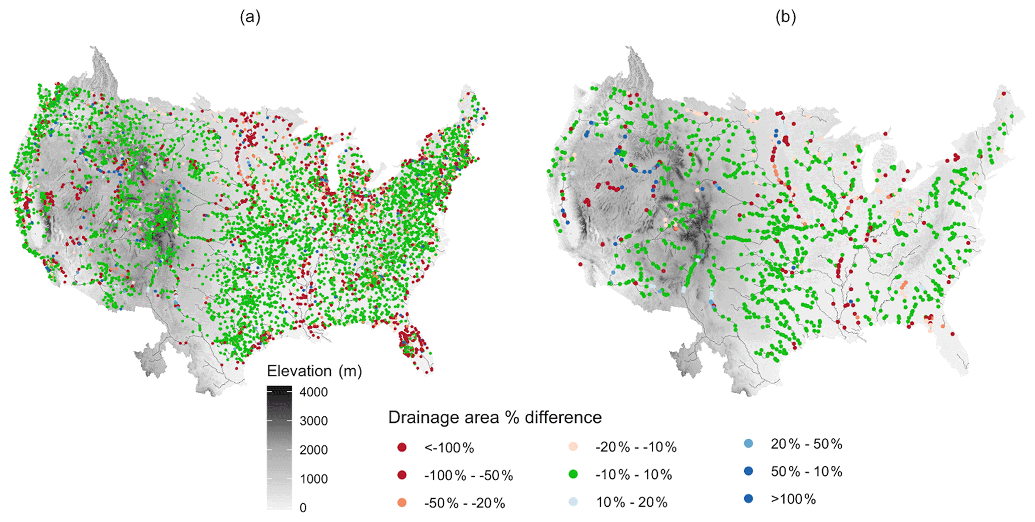
Figure 3 Drainage area comparison between processed with no initial stream network and USGS gage measurements. (a) All gages for comparison; (b) gages with drainage area over 5000 km².

To address this, we use the fifth-order stream mask to guide the topographic processing of the 1 km domain (third order for the 250 m domain). Figure 4 shows the stream gage performance maps by adding fifth-order stream mask. Adding the stream mask to processing increases the number of gages with area matches within 10 % from 5066 in the original processing without any stream mask provided to 5189 (880 to 937 for the large stream gages). Furthermore, it decreases the number of gages with area differences greater than 20 % to 204 overall and 158 among the large gages. This is a clear improvement over the processing without a stream mask. However, there are still many locations with poor drainage area matches, including large gages.

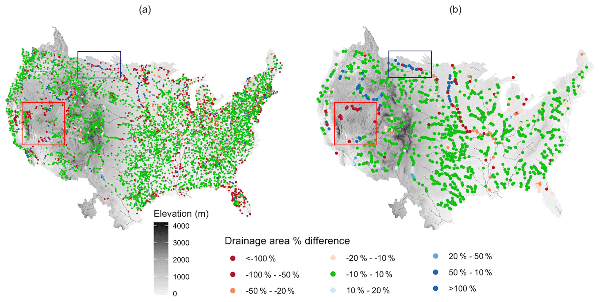
Figure 4 Drainage area comparison between processed with initial fifth-order stream network and USGS gage measurements. (a) All gages for comparison; (b) gages with drainage area over 5000 km².

Therefore, as a final step we applied a series of manual fixes to the stream network. Three primary types of fixes were applied: (1) adding sinks to the domain to increase the number of terminal points for internally draining basins, (2) manually modifying the stream mask to reflect higher-resolution information, (3) removing erroneous stream outlets that were created where the headwater cells in the stream mask intersects the boundary of the domain. This last adjustment corrected some of the anomalously high drainage areas in the norther portion of the domain (blue box in Fig. 4). For discussion purposes we will focus on the first two adjustments that impacted a much larger portion of the stream network.

Sinks were added primarily in the Great Basin portion of the domain (the red box in Fig. 4), where endorheic basins are common. This arid portion of the domain is characterized by ephemeral streams (i.e., streams that do not flow year-round) that are often poorly mapped. Figure 5 shows a portion of the Great Basin before and after sinks were added. Figure 5a shows the input topography and cells with drainage area over 10³ km² processed by the Priority Flood approach without sinks. Before sinks are added to the stream network, the Priority Flood algorithm forces all of the cells within this area to drain out, resulting in the linear stream network that does not align with the topography well and poor drainage area matching. The triangles in Fig. 5b show the sinks that were added according to the topography and fifth-order stream network. Including these as terminal points in the topographic processing improves the resulting stream network and stream gage area matches significantly. Overall a total of 262 sinks were added to the domain.

Figure 5 Panels (a) and (b) are maps illustrating the effect of sinks in drainage network derivation, a selected domain in the Great Basin (the highlighted red box in the upper-right CONUS map). In panels (a) and (b), the background is the elevation map; blue cells are the cells with drainage area over 1000 km² from processing; colored dots represent the percentage difference of drainage area between processed and USGS observations (a) without sinks and (b) with pre-defined sinks.

By far the most common manual update that was made in the processing step was to manually update the location of the stream mask. This was accomplished by visually comparing the fifth-order stream network to the higher-order streams and NHD streamlines and extending the fifth-order stream mask as needed to reflect this additional information in headwater regions. Note that simply applying a denser stream mask nationally (for example using the third-order stream mask for the 1 km domain processing) is not a viable solution here. When translated to the 1 km grid these denser stream masks result in too many grid cells being classified as stream cells and a decreased quality of the stream network overall. Therefore, we work primarily from the fifth-order stream mask but incorporate higher-resolution information as needed in an iterative process comparing our resulting drainage network to the stream gage areas. Figure 6 gives an example of a location at the northern portion of the domain where the fifth-order stream mask was expanded to improve performance of stream network derivation. Figure 6a shows the fifth-order stream network in black lines and third-order stream network in red lines. Figure 6b shows the linear drainage network that results from the initial processing with the fifth-order stream. In this flat region, it is difficult to obtain the correct drainage path with only the topographic information. By adding the third-order stream network, the drainage path presents a more reasonable pattern and an improved drainage area matching in Fig. 6c. A similar process was completed for the 250 m resolution starting from the third-order streams and extending using the second-order streams.

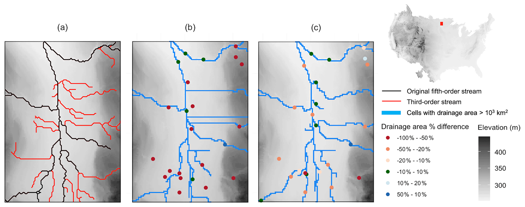
Figure 6 Panels (a), (b) and (c) are maps illustrating the impact of stream order used for the drainage mask on the resulting drainage network for a selected valley in the northern portion of CONUS (highlighted in the red box in the upper-right CONUS map). The background map is the elevation. (a) The third (red) and fifth (black) order stream network. Panels (b) and (c) are results from fifth-order stream network and third-order stream network respectively. Blue cells in panels (b) and (c) are cells with drainage area over 1000 km² after processing. Colored dots in panels (b) and (c) represent the percentage difference of drainage area between topographic processed and USGS.

Figure 7 shows the final drainage area evaluation after all the adjustments to the stream network are incorporated. Overall this demonstrates a strong improvement in the drainage area network relative to both the case with no stream network at all and the original fifth-order stream mask. Nearly all (90.0 %) of the large drainage area gages (from 880 with no stream mask to 1075 gages with the final stream mask) now have area agreements within 10 % and 74.2 % of the gages overall (from 5066 with no stream mask to 5595 gages with the final stream mask). Figure 7c summarizes the performance across the three test cases grouped by drainage area. As can be seen here, the final channel network improves performance across all drainage area categories. Performance remains most variable in the smallest drainage basins (< 100 km²). This makes sense as these are the locations where the DEM resolution will have the largest impact and also where the stream mask will have the least impact (because fifth-order streams do not extend into small headwater basins generally). Certainly, the performance of small drainage basins could be further improved with additional manual corrections to the stream network. The focus here though is on larger basins which will be most relevant for 1 km resolution hydrologic simulations.

The 250 m domain is not plotted here but is included in the processed datasets. Similar analysis of the 250 m DEM shows that, as would be expected, a higher-resolution DEM provides better information for drainage network derivation. There are 6048 gages that have area agreements within 10 % using the unmodified third-order stream mask directly from NWM. For reference this is 982 more gages than the 1 km DEM with the unmodified stream mask. Similar improvements have been found by applying all the processes to 250 m resolution. Here too the processing does not significantly improve performance for gages less than 100 km². Area agreement is enhanced vastly for gages over 500 km², and the number of gages with area agreements over 50 % decreases from 377 to 255.

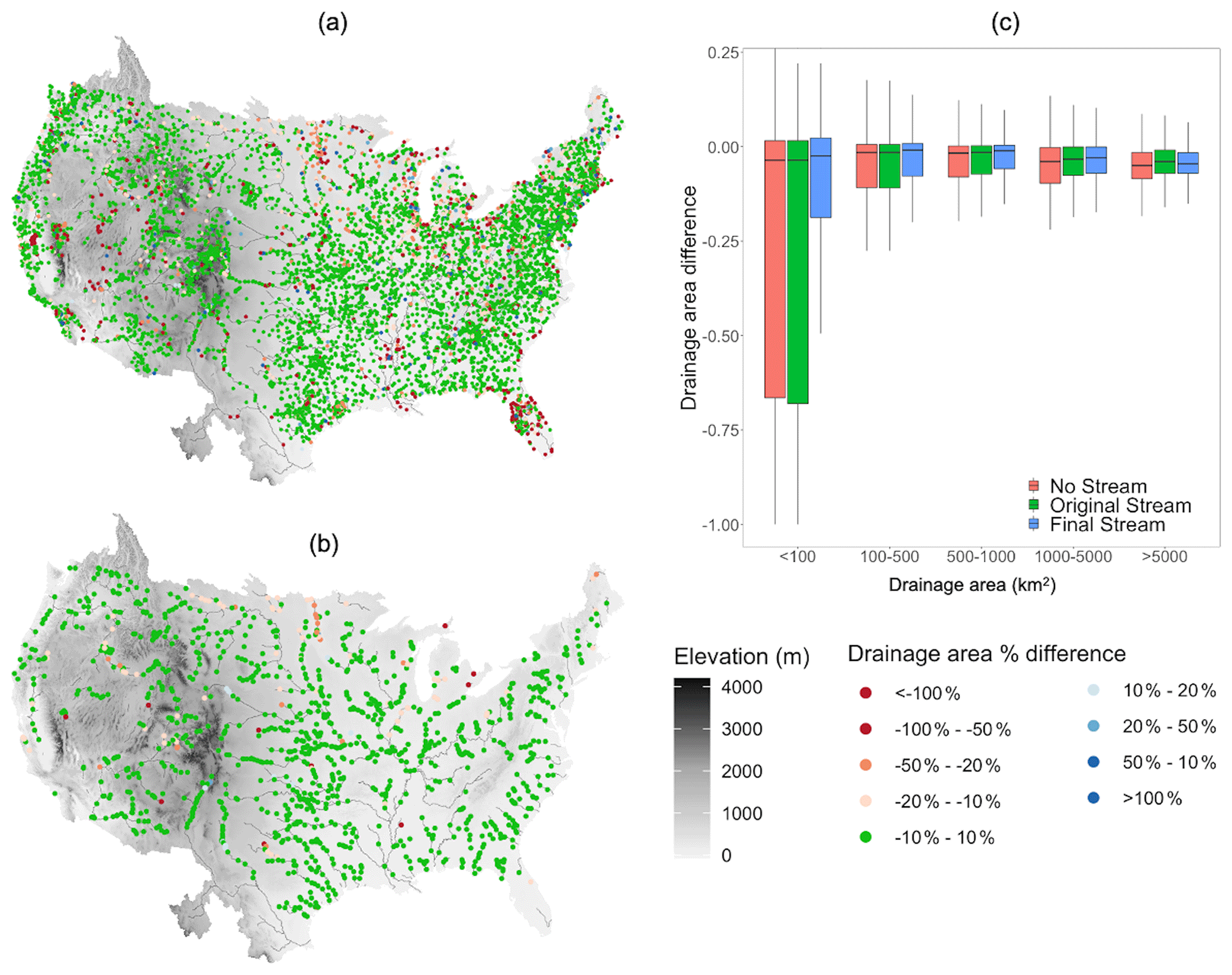
Figure 7 Drainage area comparison between processed with final-order stream network and USGS gage measurements. (a) All gages for comparison; (b) gages with drainage area over 5000 km². (c) The boxplot of drainage area difference with different stream networks grouped by drainage area size.

3.2 Drainage and overland flow performance

In addition to the drainage network location we evaluate how the topographic processing influences the runoff characteristics of the domain. As described in Sect. 2.3, this behavior is evaluated using runoff tests and assessing anomalously high ponding depths. Note that in this section we evaluate how our processing reduces ponding locations. This is not meant to imply that we are trying to get rid of all ponding in the domain. Rather we are looking for locations where the DEM resolution is leading to what we expect to be non-physically realistic ponding – specifically, discontinuities along the drainage network or anomalous locations along the hillslope. Here we consider the impact of smoothing along the stream (step 4 in the topographic processing), the flat fix step applied to the rest of the domain (step 5c in the topographic processing) and removing the secondary slope along the stream cells (step 5b in the topographic processing). For reference we compare four cases listed below with progressively more processing steps applied.

• a.

  No smooth. The slope is calculated by adjusted DEM from the Priority Flood algorithm without any stream smoothing or flat fixing.

• b.

  Add stream smooth. This consists of the no smooth case with stream smoothing added.

• c.

  Add fix flat. This consists of the add stream smooth case with the flat fix applied to the domain.

• d.

  Remove secondary. This consists of the add fix flat case with removed secondary slope along the stream cells.

Note that in all of these cases processing steps 1–3 in the topographic processing remain the same; therefore, the flow directions and location of the drainage network remain unchanged. The smoothing steps evaluated here do not alter the primary flow directions; they simply adjust the gradients along flow paths.

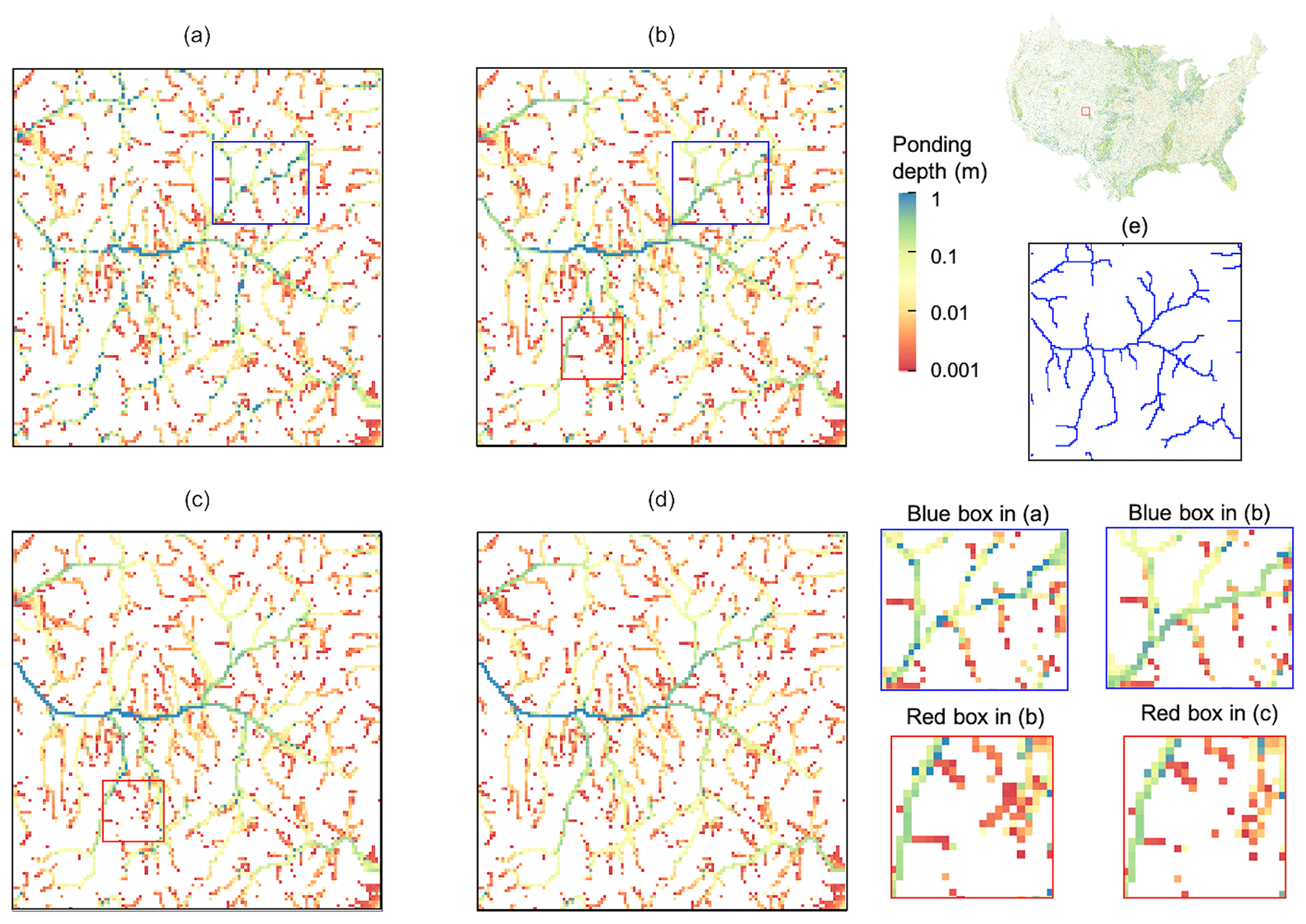
Figure 8 The ponding depth from runoff tests from four slope cases. (a) No smooth. (b) Add stream smooth. (c) Add flat fix. (d) Remove secondary. Panel (e) is the stream network from the Priority Flood approach with drainage area over 100 km². The blue and red boxes are examples to be explained in detail in the text.

Ponding depths from a small domain located in Colorado at hour 20 of the runoff test are displayed in Fig. 8 to illustrate the local impact of smoothing. The domain is 16 254 km² (126 km by 129 km), and the elevation ranges from 1601 to 4054 m. The expected stream network based on drainage area thresholds is plotted in Fig. 8e, and additional stream smoothing area is applied along the stream network.

As would be expected, the resulting stream network shape is the same, and the largest ponding depths occur along the main stem of the drainage network in all cases. What is notable in this figure though are the spatial differences in how this ponding occurs. In the no smoothing case there are discontinuities along the main stem of the stream as well as and many localized high ponding points across the domain (Fig. 8a). Applying the stream smoothing in the three subsequent cases smooths these discontinuities along the main drainage network where smoothing was applied. An example of this improvements is shown in the blue box of the domain in Fig. 8a and b and the magnified figure in the bottom-right part. Adding the flat fix step decreases the number of isolated ponding points outside the stream network (an example is shown in the red boxes in Fig. 8b and c). Note that even with this smoothing step applied there are still isolated ponding locations. This is acceptable as all cells still have the ability to drain even if it is slow and because our goal is not to achieve uniformly fast drainage everywhere. Rather the flat fix step is intended only to address those locations where large anomalies in the processed DEM result in significant ponding which may not be physically realistic. Finally, the “removed secondary slope along stream” step does not change the smoothing properties of the domain; it simply removes the secondary slope in the stream to force water in the stream drain only in the primary direction, which increases the drainage speed of stream cells.

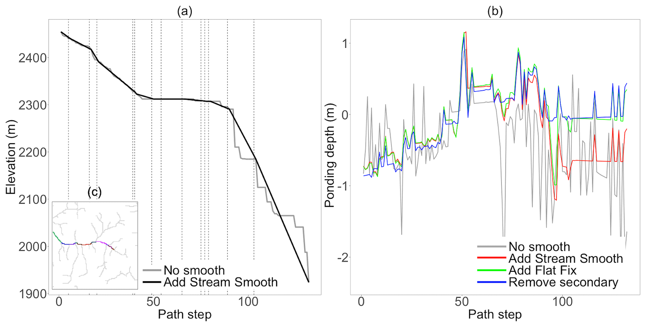
Figure 9 (a) The elevation along an example stream segment (shown in panel c) before and after smoothing applied along the stream; the stream is divided into segments by dashed lines; (b) the ponding depth along the main stem from the runoff tests with four slope cases; (c) the main stem with segments plotted by different colors

To further illustrate the impact of the stream smoothing step, Figure 9a plots the elevation along the main stem shown in Fig. 9c before and after smoothing is applied. Segments are plotted in different colors in Fig. 9c and separated by dashed lines in Fig. 9a. As can be seen here, in both cases the stream path is monotonically decreasing. However before stream smoothing is applied, there are many large steps along the stream path. With smoothing constant slopes are applied along each stream segment by adjusting the DEM along the stream. Note that the same elevation smoothing along the stream is carried out in the three smoothed test cases. Figure 9b compares the ponding depth along the stream for all four cases. Comparing the no smooth to the add stream smooth cases, it can be seen that the stream smoothing step has the largest impact on the ponding depths in the stream. Figure 9 illustrates that it significantly reduces the ponding depth variability from cell to cell. Adding the flat fix increases the ponding depth especially shown at the downstream. This is because the flat fix step increases the drainage speed of the domain as a whole, resulting in larger ponding depth in the stream. Finally, removing the secondary slope along the stream results in the smoothest pressure variation along the stream network by draining all water only to the primary direction.

The small domain shown in Figs. 8 and 9 illustrates the major behaviors seen across the domain in response to the smoothing steps. Figure 10 summarizes the results across the CONUS simulation. The background of Fig. 10 shows the ponding depth from the runoff test with the final slope at hour 20, and the barplots summarize the percentage decrease in cells with ponding greater than 0.1 m outside the main stream network after 20 h of the runoff simulation relative to the baseline, no smooth case. The stream cells are excluded from this analysis as larger ponding depth is expected in the stream network. Results are summarized by major watershed outlined in black on the figure. Still, smoothing the stream increases the drainage rate across the domain so the add stream smooth case does significantly decrease the number of ponding points outside the domain. The add flat fix case impacts a small number of cells in most basins, which is also to be expected given that it is targeting isolated discontinuities in the DEM. The flat fix step has the largest relative impact in steeper domains such as the upper Colorado due to the large variability of slopes between neighbor cells here. Removing the secondary slope has the largest impact in flatter portions of the domain such as the Mississippi Embayment.

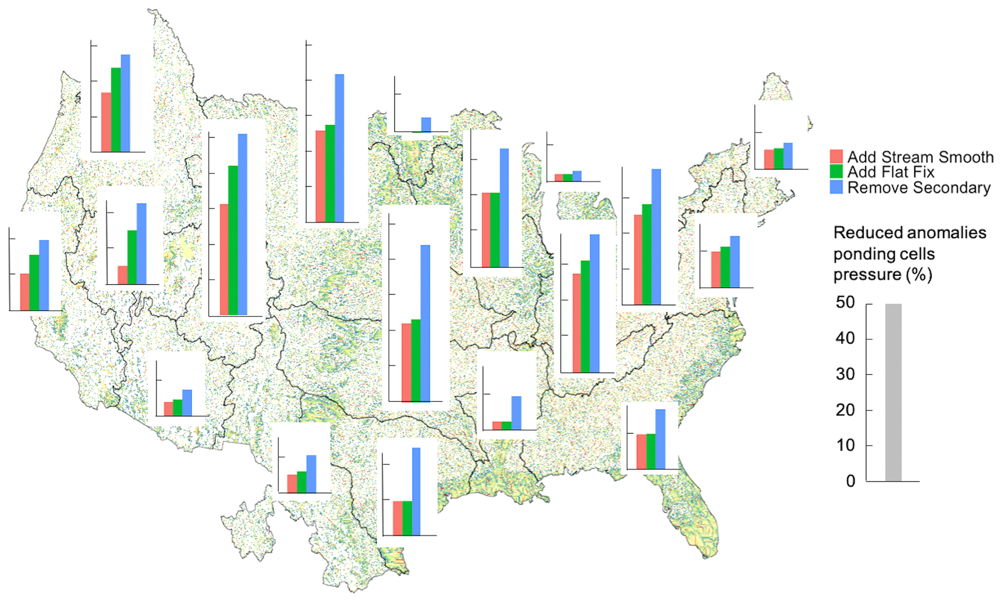
Figure 10 The background map is the ponding depth from runoff test at hour 20 with the final slope; barplots are the percentage decrease of anomalies' ponding cells (ponding depth over 0.1 m) outside the main stream network relative to the baseline (no smooth case) in HUC2s. The scale of the barplot in each HUC is the same, with the grey bar shown in the right of figure.

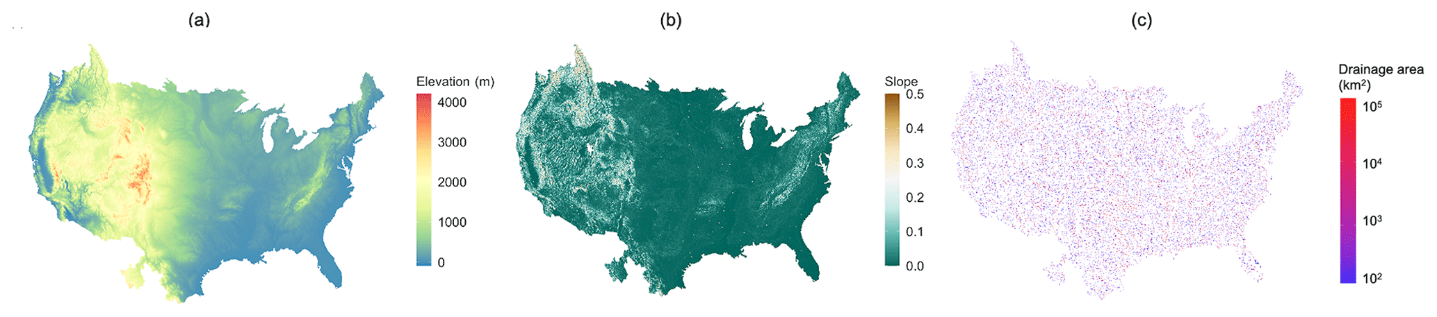
Figure 11 Demonstration of output datasets over CONUS: (a) processed DEM, (b) slope and (c) drainage area.

Table 2 Summary of gridded outputs included in the dataset.

4 Final topographic dataset

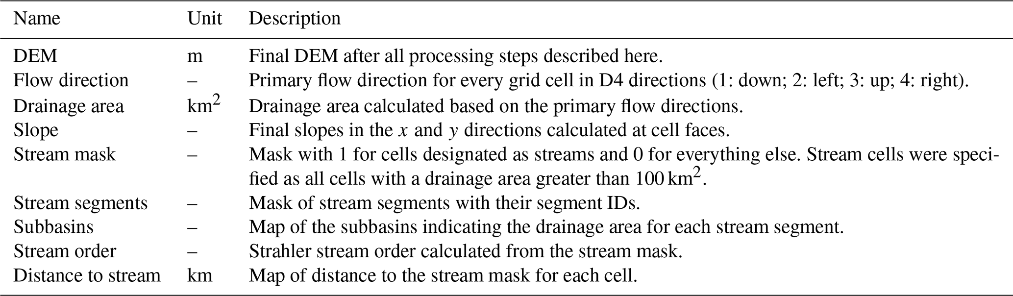
Figure 11 shows the final elevation map, slope and drainage area that result from the topographic processing. These maps plot the 1 km outputs, but all results are also available at 250 m resolution. Elevations and slopes are the primary inputs for the hydrologic modeling, but additional datasets defining the drainage networks and watersheds are also generated through the processing step (as shown by the final outputs in Fig. 2). While there are other national datasets that derive drainage networks and watersheds, we include these outputs here too because they are on the same grid and derived through the same processing steps as the DEM and therefore provide spatial information which is perfectly aligned with the final processed topography. The dataset includes a gridded map of elevation, slope in the x and y directions, primary flow directions, drainage area, stream segments, drainage basins associated with stream segments, and distance to streams. Details on each of these output datasets are listed in Table 2.

Figure 12 summarizes the differences between the final DEM of this study and the original DEM, including both the fraction of grid cells where the elevation changes and how much elevations were adjusted by. DEM adjustments are split into two categories according to the processing step where they occurred: (1) the Priority Flood adjustment step where elevations were adjusted to ensure complete drainage and (2) the subsequent smoothing steps. Results are summarized by regional hydrologic unit codes (HUC2s). The contiguous US is divided into hydrologic units identified by a unique HUC. The first level of classification divides the contiguous US into 18 major geographic regions, known as HUC2s. Overall the Priority Flood algorithm changed the elevation in 11.6 % of the grid cells, while the stream smoothing steps impacted 17.4 % of the cells. In both cases the median slope adjustment magnitude is small (1.74 m for Priority Flood and 3.12 m for smoothing). The Priority Flood algorithm frequently results in larger elevation adjustments than the stream smoothing step. Note also in Fig. 12b that the Priority Flood algorithm only increases elevations from the original to the processed DEMs, whereas the stream smoothing step can both increase and decrease elevations. Spatially the largest fraction of grid cells is adjusted in the flatter basins, for example the Mississippi Embayment (HUC 8), while the largest elevation adjustments occur in the steeper western portions of the domain such as Colorado and California (HUCs 13–18).

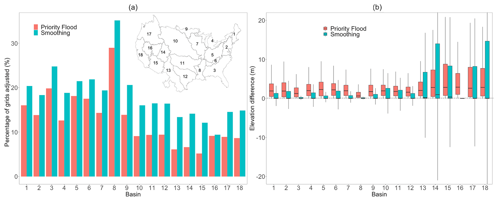
Figure 12 (a) The percentage of grids processed in two processing parts in HUC2 basins; (b) the elevation difference after the two processing parts.

5 Code and data availability

All of the topographic processing was completed with the PriorityFlow R library, which is available on GitHub (https://github.com/lecondon/PriorityFlow, last access: 5 July 2021). All of the output datasets listed in Table 2 at 250 m and 1 km resolution are published through CyVerse (DOI link: https://doi.org/10.25739/e1ps-qy48, Zhang and Condon, 2020). Datasets are available in tif, text and pfb formats. Along with these outputs, the input datasets they were generated from and the R scripts used for processing are also available. This will allow others to reproduce our work as well as generate their own versions with different processing settings if desired.

6 Conclusions

This study presents a topographic dataset developed for physically based hydrologic simulations. We combine a Priority Flood topographic processing algorithm with a priori stream network mask and USGS stream gage drainage areas to develop DEM and flow direction rasters which will closely match observed drainage networks. We also apply a series of slope smoothing steps along stream reaches and globally to improve surface runoff performance. These smoothing steps are unique from other global topographic smoothing approaches because we directly consider flow direction and stream locations to provide different smoothing along the stream reaches. The resulting DEM is designed to capture hydrologic features and improve runoff simulations for PDE-based hydrologic models which rely on gridded topography for overland flow simulations. This performance is evaluated nationally using reported drainage areas from the USGS stream gage network and runoff simulations. All outputs from the processing are available across the contiguous US at both 1 km and 250 m resolution. The processing workflow developed here uses the open-source R package PriorityFlow and is fully documented with the published datasets so that others can modify processing for different resolutions or specific subdomains as desired.