the Creative Commons Attribution 4.0 License.
the Creative Commons Attribution 4.0 License.
 | 07 Jul 2021
A fine-resolution soil moisture dataset for China in 2002–2018
Xiangjin Meng
Fei Meng
Jiancheng Shi
Jiangyuan Zeng
Xinyi Shen
Yaokui Cui
Lingmei Jiang
Zhonghua Guo
Soil moisture is an important parameter required for agricultural drought monitoring and climate change models. Passive microwave remote sensing technology has become an important means to quickly obtain soil moisture across large areas, but the coarse spatial resolution of microwave data imposes great limitations on the application of these data. We provide a unique soil moisture dataset (0.05∘, monthly) for China from 2002 to 2018 based on reconstruction model-based downscaling techniques using soil moisture data from different passive microwave products – including AMSR-E and AMSR2 (Advanced Microwave Scanning Radiometer for Earth Observing System) JAXA (Japan Aerospace Exploration Agency) Level 3 products and SMOS-IC (Soil Moisture and Ocean Salinity designed by the Institut National de la Recherche Agronomique, INRA, and Centre d’Etudes Spatiales de la BIOsphère, CESBIO) products – calibrated with a consistent model in combination with ground observation data. This new fine-resolution soil moisture dataset with a high spatial resolution overcomes the multisource data time matching problem between optical and microwave data sources and eliminates the difference between the different sensor observation errors. The validation analysis indicates that the accuracy of the new dataset is satisfactory (bias: −0.057, −0.063 and −0.027 m3 m−3; unbiased root mean square error (ubRMSE): 0.056, 0.036 and 0.048; correlation coefficient (R): 0.84, 0.85 and 0.89 on monthly, seasonal and annual scales, respectively). The new dataset was used to analyze the spatiotemporal patterns of soil water content across China from 2002 to 2018. In the past 17 years, China's soil moisture has shown cyclical fluctuations and a slight downward trend and can be summarized as wet in the south and dry in the north, with increases in the west and decreases in the east. The reconstructed dataset can be widely used to significantly improve hydrologic and drought monitoring and can serve as an important input for ecological and other geophysical models. The data are published in Zenodo at https://doi.org/10.5281/zenodo.4738556 (Meng et al., 2021a).
- Article
(19146 KB) - Full-text XML
- BibTeX
- EndNote


Soil moisture (SM), which is one of the key variables in water cycle and atmospheric energy budget (Taylor et al., 2011; Shi et al., 2012; Guillod et al., 2015), has been widely used for flood forecasts (Bindlish et al., 2009), drought detection (Mao et al., 2010, 2012), crop yield estimation (Chen et al., 2011), weather prediction and hydrological modeling (Liu et al., 2017). Therefore, accurately monitoring and assessing the dynamics of the spatiotemporal distribution of SM are crucial for understanding the hydrological, ecological and biogeochemical processes associated with global and regional climate systems (Mao et al., 2008a, b; Seneviratne et al., 2010; Han et al., 2012; Wang et al., 2016). The most direct way to obtain SM is primarily from in situ measurements with SM measuring instruments at ground meteorological stations (Franz et al., 2012). SM networks based on ground stations have made great contributions to establishing long-term SM datasets (Srivastava, 2016). The in situ SM observations from these networks have also been unified into a common database (Dorigo et al., 2011). However, accurate measurements of SM are limited by the number of field sites, and measuring SM at a single location does not necessarily represent the condition of an entire region due to the large spatial heterogeneity of SM (Crow et al., 2002; Njoku and Entekhabi, 1996, 2003). With the development of remote sensing technology, satellite-based SM measurements have become one of the most effective and rapid methods to obtain large-scale SM (Loew and Schlenz, 2011; Petropoulos et al., 2015; Srivastava, 2017). Microwave remote sensing, including active microwave and passive microwave, has become the most effective means of monitoring SM (Schmugge et al., 1974; Moran et al., 2004; Shi et al., 2006; Shen et al., 2013; Bhagat, 2014) and has been used to provide global coverage for surface SM datasets (Njoku et al., 2003; Albergel et al., 2013). The European Space Agency's Water Cycle Multi-Mission Observation Strategy (ESA WACMOS) Support to Science Element (STSE) program has developed the first long-term SM data record from passive and active microwave data (Su et al., 2010). In 2012, the ESA's Climate Change Initiative (CCI) program SM datasets were first publicized on the ESA CCI web portal. This CCI product was generated by merging different microwave sensor observations and attempting to produce a complete and consistent long-term time series of SM datasets (Dorigo et al., 2017; Gruber et al., 2019). Kang et al. (2020) improved the algorithm for FY-3D microwave data and also produced a global SM product (Kang et al., 2020), and the resolution is about 0.25∘ covering 2017–2019. Chen et al. (2021) developed a novel spatiotemporal partial convolutional neural network (CNN) for AMSR2 soil moisture product gap-filling, and the resolution is about 0.25∘ covering 2003–2019. The long-term availability of SM products has been validated against extensive model simulations and in situ measurements (Albergel et al., 2012; Loew et al., 2013; Zeng et al., 2015; Dorigo et al., 2015, Preimesberger et al., 2021).
Although the SM datasets mentioned above can provide SM parameters for global climate change research, the resolution is relatively low (e.g., 10 or 25 km), which makes it very difficult to meet local refined research, especially agricultural drought monitoring. In order to obtain a soil moisture dataset with high spatial resolution, various methods have been proposed to downscale SM (Liu et al., 2009, 2011; Sandholt et al., 2002; Peng et al., 2015; Mohanty et al., 2017). The basic principle of most methods is that the drought index constructed using high-resolution visible light and thermal infrared data has a strong linear relationship with microwave soil moisture in local areas (Moran et al., 1994; Carlson et al., 1994; Jin et al., 2017; Maltese et al., 2015; Wang et al., 2016). The temperature vegetation dryness index (TVDI) was developed to estimate the SM (Sandholt et al., 2002; Choi and Hur, 2012), which is the most classic method and has been widely used for the downscaling of microwave SM and drought monitoring over different regions (Chauhan et al., 2003). Jing et al. (2018) proposed a two-step reconstruction approach for reconstructing satellite-based soil moisture product essential climate variables (ECVs) at an improved spatial resolution of 0.05∘ covering 2001–2012. The reconstruction model implemented the random forest (RF) regression algorithm to simulate the relationships between soil moisture and environmental variables, and it takes advantage of the high spatial resolution of optical remote sensing products (Jing et al., 2018). Most downscaling datasets are mainly made for a single sensor. Due to the limitation of the lifetime of satellite sensors, the time series is not long enough, and it is difficult to analyze the temporal and spatial changes in a long time series. Different satellite microwave sensors have differences in time and space, and the depth information of SM detected by the different frequencies of different microwave sensors is not consistent. In order to obtain a longer time sequence in an SM dataset, we must eliminate the differences between different sensors (Peng et al., 2017). Many methods have been proposed to handle these systematic differences among SM products from different microwave sensors (Zwieback et al., 2016). Recent studies have exploited the utility of rescaling SM product methods (Brocca et al., 2013; Zeng et al., 2020). Linear regression rescaling of SM has proven to be a simple and effective method, and a review of these rescaling methods was published by Afshar and Yilmaz (2017). To produce a soil moisture dataset with high spatial and temporal resolution, the similarity of microwave sensors must be considered, and the high-resolution visible light and thermal infrared data must be synchronized as much as possible. Few satellites meet these conditions at the same time. The Aqua satellite, which is equipped with both the Advanced Microwave Scanning Radiometer for Earth Observing System (AMSR-E) and the Moderate Resolution Imaging Spectroradiometer (MODIS) sensors, can simultaneously provide coarse-resolution passive microwave SM, land surface temperature (LST) and normalized difference vegetation index (NDVI) data, which guarantees that the data were acquired at the same time. However, AMSR-E data alone are insufficient (the instrument stopped working in October 2011), and its successor AMSR2 can be used to continue the data series. The missing data between AMSR-E and AMSR2 (from November 2011 to June 2012) can also be supplemented by SMOS-IC (Soil Moisture and Ocean Salinity designed by the Institut National de la Recherche Agronomique, INRA, and Centre d’Etudes Spatiales de la BIOsphère, CESBIO) data, which have been validated with high accuracy by using in situ measurements (Al-Yaari et al., 2019; Ma et al., 2019).
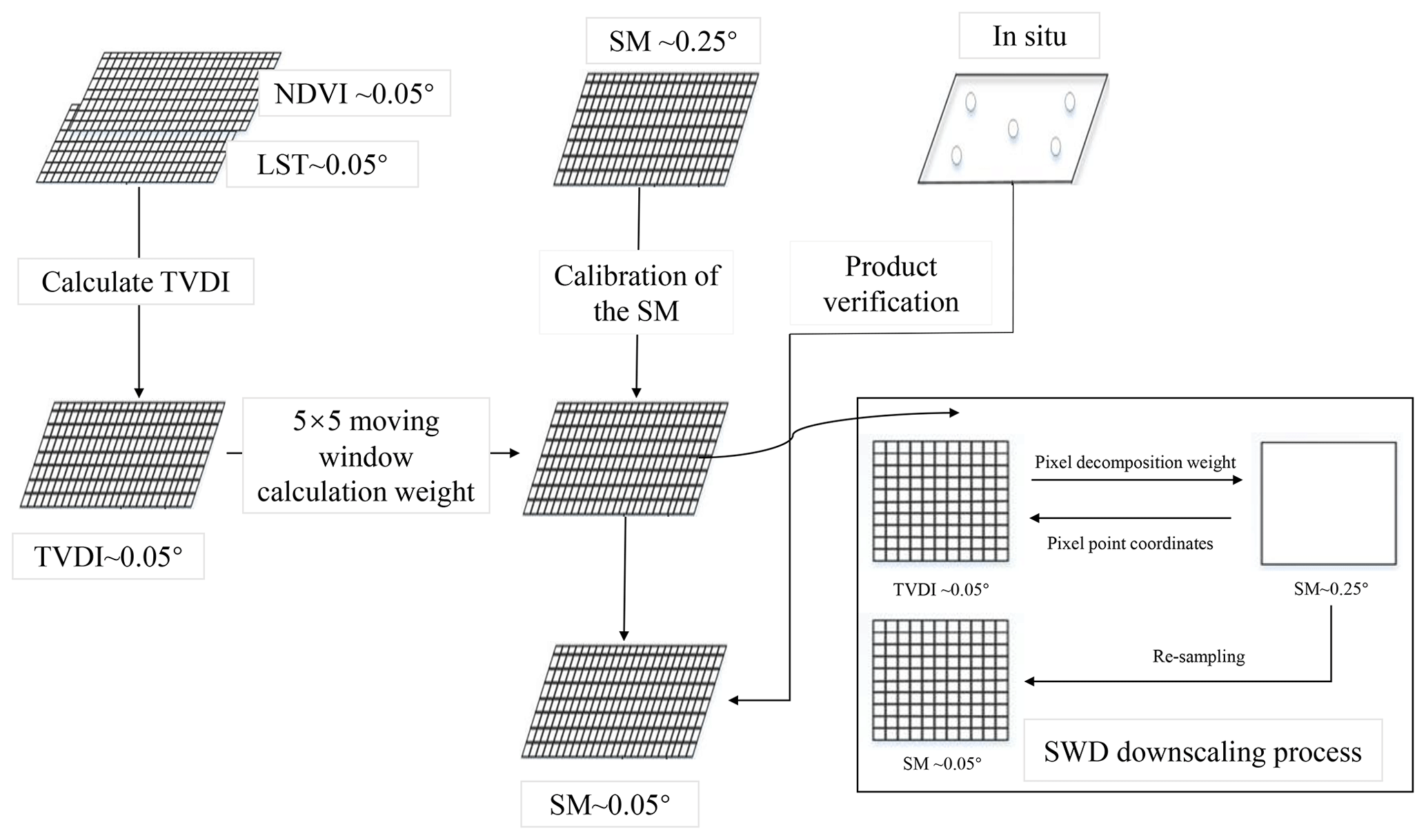
In this study, in order to obtain a SM dataset with higher spatiotemporal resolution and higher consistency, all microwave SM data are based on AMSR-E Level 3 data, uniformly corrected to the same time and the same depth of detection using a linear regression method. In addition, ground station data are incorporated, and a large area of missing and invalid pixels is restored so that the entire dataset can be guaranteed to be complete in the Chinese region. A spatial downscaling method, namely the spatial weight decomposition (SWD) model, was utilized to decompose the coarse-spatial-resolution SM products with the TVDI method into SM data with 0.05∘ spatial resolution. The dataset covers the period from 2002 to 2018 and is comprehensively compared with in situ SM datasets.
China is located in central and eastern Asia on the west coast of the Pacific Ocean, is affected by the monsoon climate and has important monsoon climate characteristics. Drought disasters in China have constantly increased over recent years, which has become one of the most serious types of natural disasters. The rapid increase in industry, irrigation and domestic water use has led to a dramatic increase in water consumption, which in turn has led to a sharp increase in drought in most parts of China, especially in northern China (Zhao et al., 2017). Thus, there is an urgent need to improve our knowledge about the spatial and temporal variability of SM to provide a basis for quantification and prediction, especially for the management of agricultural water (Liu et al., 2012). Hence, it is necessary to construct a set of high-precision and high-spatial-resolution SM datasets in China.
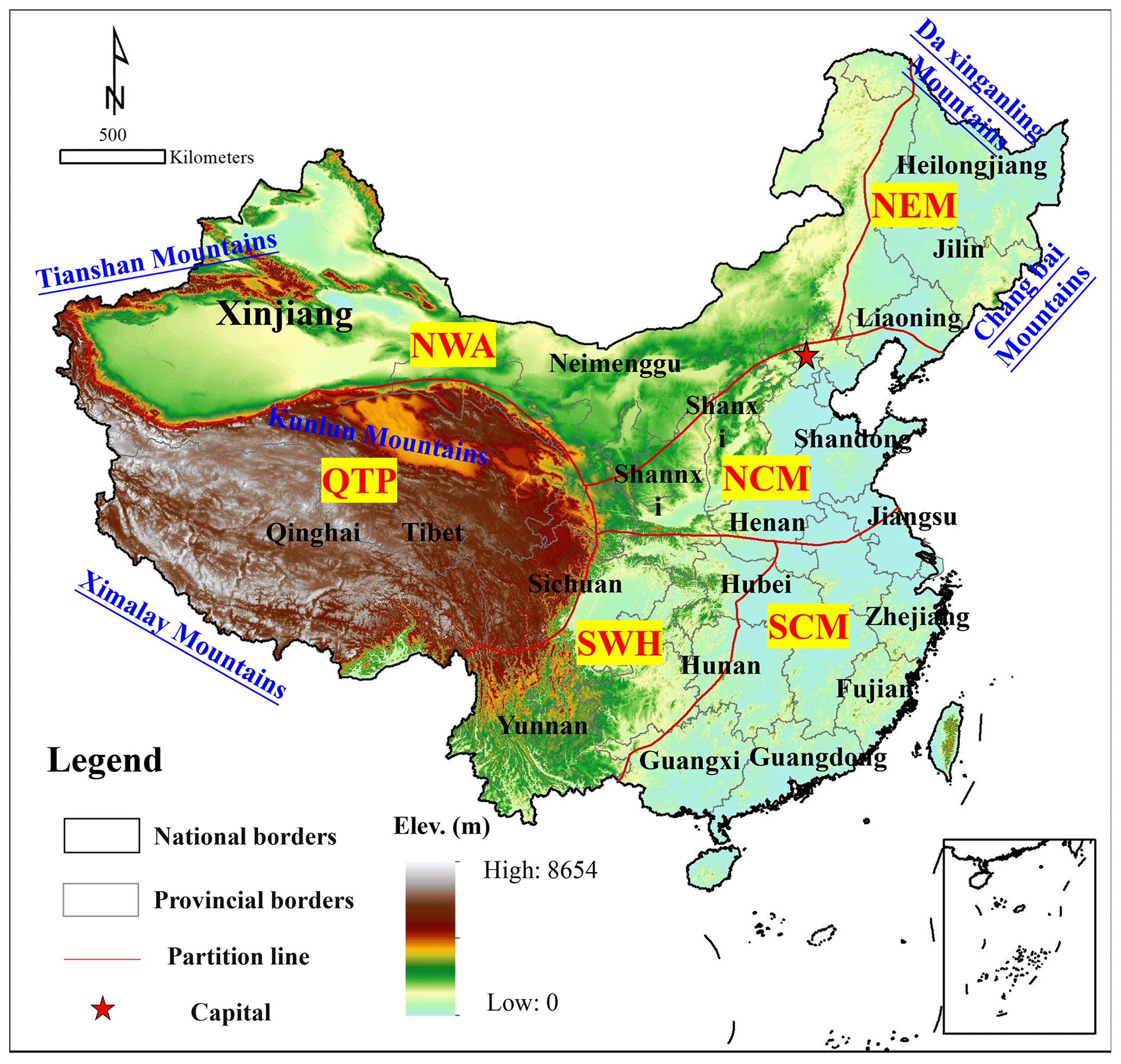
Figure 1Overview of the study area and six geographic-climatic regions in China. The base map is derived from the Resource and Environment Science and Data Center of the Chinese Academy of Sciences (http://www.resdc.cn/, last access: 16 November 2019).
To improve the quality of SM dataset and explore the spatial and temporal patterns of SM throughout the various regions of China, we further divided China into six regions based on conditions such as elevation, rainfall, topography and hydrogeology combining hydrogeologic features: Northeast Monsoon Region (NEM), North China Monsoon Region (NCM), South China Monsoon Region (SCM), Southwest Humid Region (SWH), Northwest Arid Region (NWA) and Qinghai–Tibet Plateau Region (QTP) (Liang et al., 2017). The NEM includes the areas to the south of the Heilongjiang River, to the east of the Daxing'anling mountain range and to the north of the Ming Great Wall (38–53∘ N, 117–135∘ E). The North China Monsoon Region, which extends from the Inner Mongolian Plateau to the northern part of the Qinling–Huaihe River, east to the eastern part of the Yellow Sea and the Bohai Sea, and west to the eastern part of the Qinghai–Tibet Plateau, has typical temperate monsoon climate characteristics (33–42∘ N, 103–125∘ E). The South China Monsoon Region includes the monsoon region to the east of the Yunnan–Guizhou Plateau and to the south of the Qinling Mountains–Huaihe River. This region has abundant rainfall and dense river networks and is characterized by a typical subtropical monsoon climate (105–123∘ N, 20–33∘ E). The Southwest Humid Region includes the Qinghai–Tibet Plateau and the Yunnan–Guizhou Plateau to the south of the Huaihe River and the Sichuan Basin. Precipitation is abundant in southwestern China (97–104∘ N, 21–34∘ E). The Northwest Arid Region includes the Inner Mongolian Plateau to the east of the Greater Xing'an Mountains and the vast arid and semiarid regions of northwestern China in the Tarim Basin to the north of the Qinghai–Tibet Plateau (37–55∘ N, 73–126∘ E). The Qinghai–Tibet Plateau Region includes the southern part of the Kunlun Mountains–Altun Mountains–Qilian Mountains, the area to the west of the Hengduan Mountains and the entire Qinghai–Tibet Plateau to the north of the Himalayas (27–40∘ N, 73–104∘ E; Zhao and Chen, 2011). The locations of the meteorological stations and six geographic-climatic regions in China are shown in Fig. 1.
3.1 Satellite-derived SM data
Since satellite sensors have a limited lifespan, to obtain a longer sequence of SM datasets, we need to use different satellite sensors to generate unbroken SM products. The SM data are mainly derived from the AMSR-E and AMSR2 Level 3 and SMOS-IC with spatial resolutions of 0.25∘. AMSR-E is on board the Aqua satellite (effective service period from May 2002 to October 2011) with transit times of 13:30 and 01:30, and the orbit is a sun-synchronous near-polar orbit with an orbital height of approximately 700 km (Kim and Hogue, 2012; Rüdiger et al., 2009), which has six wavelengths in the microwave spectrum (6.925, 10.65, 18.7, 23.8, 36.5 and 89 GHz). The SM data utilized in this study were obtained from the Japan Aerospace Exploration Agency (JAXA) AMSR-E SM L3 product (Koike et al., 2004), and the time series ranges from July 2002 to September 2011. This product is based on the JAXA algorithm and is posted with a 0.25∘ spatial resolution. First, a forward radiative transfer scheme is used to establish a brightness temperature dataset for a variety of frequencies and polarization-generated parameter values (soil and vegetation). Then, the brightness temperature dataset is used to create a lookup table (LUT). Finally, the SM and vegetation water content are estimated by using the microwave polarization difference index (MPDI) at 10.65 GHz and the index of soil wetness (ISW) at 36.5 and 10.65 GHz horizontal channels (Koike et al., 2004). The JAXA algorithm assumes that the optical depth of vegetation is linearly related to the vegetation water content and that the vegetation water content can be determined by the NDVI. Based on verification with the ground monitoring network, JAXA products provide acceptable SM results (Draper et al., 2009; Zeng et al., 2015).
The AMSR2 sensor is mounted on the Japanese Global Change Observation Mission – Water Satellite 1 (GCOM-W1) and was launched in May 2012. As a follow-up to AMSR-E, AMSR2 has a larger antenna reflector diameter, increasing from 1.6 to 2.0 m. Moreover, AMSR2 includes an extra C-band channel (with a frequency of 7.3 GHz) to mitigate radio frequency interference (RFI). The transit times are still 13:30 and 01:30. The data were derived from the JAXA SM products, which were released in real time, and the time span ranges from July 2012 to December 2018. As a continuation of the AMSR-E product, the AMSR2 L3 product also uses a LUT method to obtain SM retrievals, providing two products with spatial resolutions of 0.1 and 0.25∘. To better match the available data, this paper selects the data with a spatial resolution of 0.25∘. The accuracy of the JAXA AMSR2 product was verified to have a root mean square error (RMSE) of less than 0.06 m3 m−3 (for a vegetation water content of ≤ 1.5 kg m−2; Kim et al., 2015).
The SMOS satellite was launched on 2 November, 2009, and it travels along a sun-synchronous orbit with an average altitude of 758 km and a dip of 98.44∘. The transit times are approximately 06:00 (ascending) and 18:00 (descending) (all times are local solar time) with a 2 to 3 d revisit frequency. The operating L-band (1.4 GHz), measured with the Microwave Imaging Radiometer with Aperture Synthesis (MIRAS), is used to observe SM (Kerr et al., 2012; Lacava et al., 2012; González-Zamora et al., 2015). This study uses the SMOS-IC V105 SM product contributions from the Centre Aval de Traitement des Données SMOS (CATDS), with a time series ranging from October 2011 to June 2012 and a spatial resolution of 25 km. The SMOS-IC algorithm was designed by the Institut National de la Recherche Agronomique (INRA) and Centre d'Etudes Spatiales de la BIOsphère (CESBIO) (Fernandez-Moran et al., 2017). The SMOS-IC product was further quality filtered and redivided based on the previous SMOS Level 2 SM user data product (SMDUP2) algorithm. That is to say that the values of the grid point data quality index (DQX) greater than 0.07 which were affected by RFI or SM were discarded. Then, the DQX reverse-weighted average was used to group the SMDUP2 data on a 0.25∘ equal-area grid and obtain SMOS-IC-grade products with a 25 km spatial resolution. Al-Yaari et al. (2019) and Ma et al. (2019) conducted comprehensive evaluations of the SMOS-IC SM product by using ground measurements worldwide. The results showed that the SMOS-IC SM product agreed better with in situ measurements than other SMOS products (SMOS L2 and L3). The SMOS-IC scientific data were as independent as possible from auxiliary data, and the data are available at https://www.catds.fr/Products/Available-products-from-CEC-SM/SMOS-IC (last access: 29 April 2020). The data are provided on a daily timescale to match the AMSR-E and AMSR2 L3 SM products at the same scale. The SMOS-IC SM data were aggregated to a monthly temporal resolution.
3.2 MODIS LST and NDVI data
For a downscaling model, it is critical to establish the relationships between SM and other high-resolution surface variables. Im et al. (2016) utilized the relationships between SM and MODIS-derived products to improve the resolution of the AMSR-E SM product. Wang et al. (2016) downscaled SM data from a 0.25∘ resolution to a 0.05∘ resolution using a similar approach. Zhao et al. (2018) used the vegetation–thermal relationship to establish a microwave–optical and infrared downscaling model to optimize the spatial resolution of Soil Moisture Active Passive (SMAP) SM products to a very good level of precision. All these land surface variables are available from the corresponding MODIS products. The MODIS sensor on board the Aqua satellites passes over China at approximately 01:30 (descending) and 13:30 (ascending). MODIS has been widely used to monitor various environments, including land, oceans and the lower atmosphere, due to its high temporal resolution and good data quality. In this study, two MODIS products were used, namely, the MODIS/AQUA monthly LST (MYD11C3) and NDVI (MYD1C2) products, which have 0.05∘ spatial resolutions, to ensure the same transit time as the microwave SM data. The MODIS products were downloaded from the NASA Land Processes Distributed Active Archive Center (LPDAAC) at the United States Geological Survey (USGS) (https://lpdaac.usgs.gov/, last access: 1 November 2020). For consistency with the SM data, all data were averaged by day and night products, and outliers were eliminated by the first-order difference method. Furthermore, null values were interpolated using the Savitzky–Golay (S–G) filter.
3.3 Meteorological and auxiliary data
SM data from the China's national meteorological stations (CNMSs) and China's agrometeorological and ecological observation network (http://data.cma.cn/, last access: 16 November 2019) were used to validate the downscaled SM products. We used the hourly in situ SM data measured at 0–10 cm depth to investigate the accuracy of the satellite-derived surface SM estimates. Monthly products were obtained from 2420 agrometeorological stations (including Key Stations of the National Climate Observatory, Basic Stations of the National Meteorological Observatory and General Stations of the Regional Meteorological Stations). Based on the nearest neighbor data during the daily satellite transit, and aggregated into monthly products through averages to match the satellite downscaled SM products, shown in Fig. A1 for site space locations. The AMSR series satellites used in this research are taken as an example. The daily transit times of the satellites in China are 13:30 and 01:30. Therefore, the ground SM measurements in daytime (13:00 and 14:00) and nighttime (01:00 and 02:00) are averaged. In the aggregation calculation, abnormal and unrepresentative data are eliminated to ensure that the selected data can reflect all the physical conditions that affect the remote sensing signal. The China Ecosystem Research Network (CERN) has locations in different regions of the study area and records different surface and climatic conditions, which are used to validate the downscaled SM deviation in different land cover types.
In addition to the above data, the Shuttle Radar Topography Mission (SRTM) of the USGS (https://lpdaac.usgs.gov/, last access: 18 May 2021) provides digital elevation model (DEM) data with a resolution of 1 km resampled to 0.05∘. These data were used to obtain terrain factors (e.g., elevation and slope) for the downscaling studies.
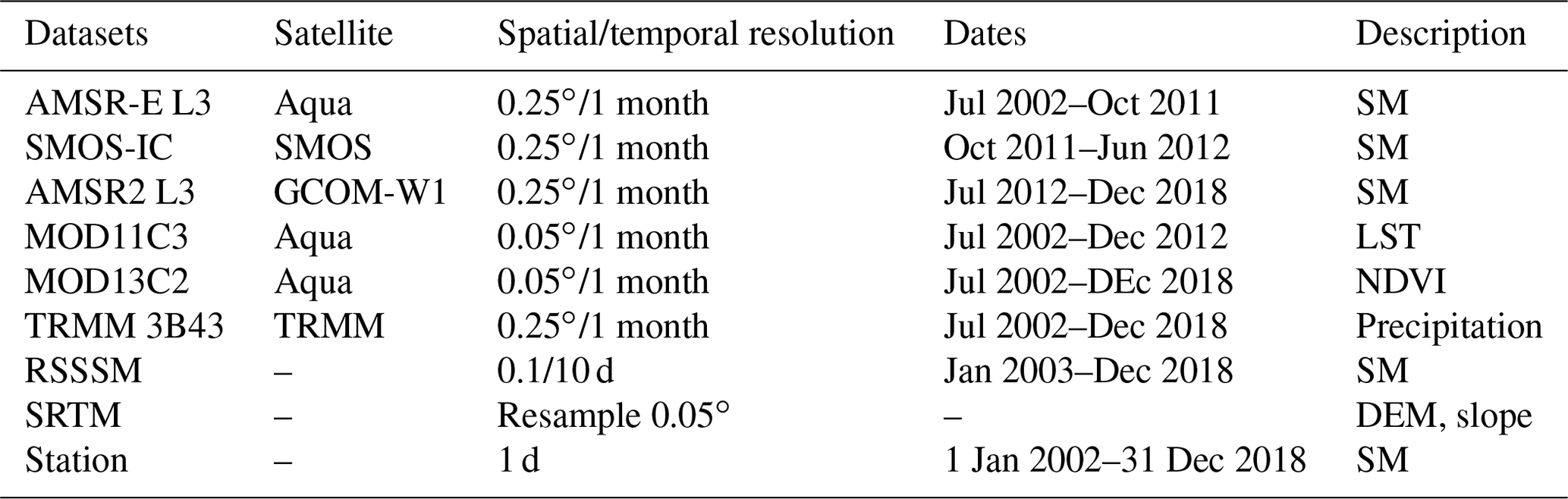
The Tropical Rainfall Measuring Mission (TRMM) 3B43 precipitation and Chen et al. (2021) developed a global remote-sensing-based surface soil moisture (RSSSM) dataset to assist in assessing the quality of downscaled products. Table 1 lists an overview of the main datasets and a description of the corresponding variables for each dataset in this study. According to the seasonal division of weather, spring ranges from March to May, summer from June to August, autumn from September to November and winter from December to February.
3.4 Methodology
3.4.1 Calibration and restoration of the satellite-derived SM
The microwave frequency and overpass time of the satellite are two important factors for deriving SM values (Cashion et al., 2005). In theory, the surface SM data retrieved from different frequencies have different soil sampling depths (Njoku and Entekhabi, 1996; Owe and Van de Griend, 1998). The diurnal variations in SM and temperature may be considerable in some regions, so the overpass time of the sensor can influence the retrieved SM. AMSR-E and AMSR2 have the same ascending and descending overpass times, i.e., 13:30 and 01:30. The SMOS SM retrievals occur at dawn and nightfall, corresponding to the SMOS ascending and descending overpass times at 06:00 and 18:00. Differences in the overpass time and observed depth of the sensors could be serious issues when matching data, particularly when deriving long-term trends. Hence, the impact of differences among sensors is considered in this study. Although SM measurements retrieved from AMSR-E and AMSR2 and SMOS have some differences, they show similar seasonal patterns, which provides the possibility for calibrating and rescaling to yield a long-term dataset. AMSR-E was selected as the reference because it is associated with a relatively long time series. The linear regression matching technique was chosen as the calibration method. Similar matching approaches have been successfully used in the past. Crow and Zhan (2007) rescaled satellite SM observations with a model by linear regression matching, and Brocca et al. (2013) also established regression relationships between satellites and in situ observations for the calibration of satellite SM observations using regression matching. In general, the linear rescaling method is realized by considering the most general linear relationship between the reference dataset (X) and the original dataset (Y). In this study, the linear regression method is applied cell by cell and its form is Eq. (1).
where μX and μY are the average values of X and Y to calculate the sequence, respectively. Y∗ is the scaled value of the original data Y, and CY is a scalar scaling factor. We eliminate the impacts of different observation times in the fitting process. Here is a linear method proposed by Yilmaz and Crow (2013) to determine the size of CY, and CY is calculated with Eq. (2).
where ρXY is the correlation coefficient of X and Y, and σX and σY are the standard errors of X and Y, respectively. The calibration procedure is applied to monthly averages of SMOS-IC data. The SMOS-IC values are plotted against the AMSR-E values for the overlapping period (July 2002 to October 2011) to calculate calibrated parameters (linear equations), and then calibrating equations derived from the previous step are applied to SMOS-IC data for the period from 2011 through 2012, producing calibrated SMOS data (SMOSreg refers to the calibrated values). The AMSR2 values are calibrated against the SMOS-IC values using data from the overlapping period. The equations derived from the previous step are used to calibrate the AMSR2 data from the period 2012–2018, producing AMSR2reg. The AMSR-E, SMOSreg and AMSR2reg data are thus obtained from 2002 to 2018.
3.4.2 Downscaling method for SM
Based on the identification of a negative correlation between the SM products and LST and NDVI (Rahimzadeh-Bajgiran et al., 2012), we construct an efficient downscaling process in which the TVDI is a weighting factor for downscaling. First, we computed the fault and null value areas based on the Savitzky–Golay filter to eliminate the effects of clouds and water vapor on the MODIS LST/NDVI images. Then, we build an LST terrain correction model to reduce the influence of terrain fluctuations on the surface temperature inversion results. In addition, we establish a monthly TVDI distribution using the LST/NDVI inversion model based on LST and NDVI images acquired from MODIS at 0.05∘ spatial resolution. Finally, we construct an SWD model to decompose the SM pixel by pixel and generate a monthly 0.05∘ SM gridded product. A structural diagram of the method is given in Fig. 2.
Since visible light and thermal infrared remote sensing are greatly affected by clouds and harsh atmospheric conditions, there is a lack of continuous LST and NDVI data. To compensate for the error caused by insufficient MODIS data, the first-order difference method is used to eliminate outliers, and the Savitzky–Golay (S–G) filter is then used to reconstruct the time series data from 2002 to 2018 and to interpolate the null values of the missing data. The specific method is shown in Eq. (3).
where represents the time series data after the supplementation. is equal to half the size of the smoothing window. Ci is the fitting coefficient of the Savitzky–Golay polynomial filter, i.e., the weight of the ith value from the filter head, and N is the length of the data processed by the filter (the number of data points contained in the sliding window).
Due to the large elevation variations in China, the influence of terrain on temperature must be corrected before the TVDI can be calculated. In order to make up for missing values and reduce the influence of terrain fluctuations on the temperature data, Eq. (4) is used approximately to repair missing temperature values in areas with large terrain differences, as described in previous studies (Molero et al., 2016, Yan et al., 2020, Zhao et al., 2020).
where Tm is the corrected temperature, To is the temperature before correction, h is the elevation value at a certain pixel, and λ is the average influence coefficient of the elevation on the surface temperature inversion process (where the value of λ is about 0.006 ).
The TVDI calculation formula, which was proposed by Sandholt et al. (2002), can adequately estimate the surface water conditions of soil. Thus, the TVDI has been widely used in drought monitoring, and the TVDI expression is shown in Eqs. (5)–(7).
where Ts is the LST (∘C) in the study area, Ts min is the LST of the wet side, (a2, b2) is the simulation coefficient of the “wet edge” model, Ts max is the surface temperature of the dry side, and (a1, b1) is the simulation coefficient of the “dry edge” model.
Based on the LST/NDVI feature space, many studies have shown that the TVDI exhibits a significant negative correlation with SM (Wang et al., 2016). The high-resolution TVDI distribution is used to weight the low-resolution SM data pixel by pixel, and then the weight is used to decompose the low-spatial-resolution SM product into 0.05∘ SM products. The SWD is computed by Eq.(8).
where SMi represents the downscaled SM with 0.05∘ pixels. SMj represents the input low-resolution microwave SM with 0.25∘ pixels. TVDIa is the TVDI value calculated using the MODIS, and TVDIb is the TVDI average MODIS pixels corresponding to the area of microwave observations of SM.

Figure 3Correlations between the downscaled SM and in situ SM measurements at the (a) monthly, (b) seasonal and (c) annual scales. The solid lines are the trend lines, and the dashed lines are the y=x reference lines.
3.4.3 Evaluation metrics of downscaled SM
It is necessary to evaluate the SM downscaling results before further application. The accuracy of the fine-spatial-resolution SM is evaluated in terms of R, bias and unbiased RMSE (ubRMSE) (Ma et al., 2019).
where Ti is the downscaled SM value in the ith year. Li is the in situ SM value in the ith year. T and L are the mean downscaled and in situ SM values, respectively. N represents the total number of observations, and σT and σL represent the standard deviations of the downscaled and in situ SM values, respectively.
4.1 Validation of the downscaled soil moisture datasets
Figure A2 shows the SM images before and after downscaling in June 2002 and the value of cross-sectional pixels. The results of downscaled SM products using spatial weights not only retain the spatial distribution of the original images but also has more spatial details. Before applying the downscaled SM products, the downscaled high-spatial-resolution SM productions are first validated against the in situ observations of CNMSs over China at three temporal scales. Figure 3a displays the scatterplots between monthly downscaled SM and measured SM, and the downscaled SM agrees well with the ground-measured SM with a correlation coefficient (R) of 0.84, and the bias and ubRMSE are −0.057 and 0.056 m3 m−3, respectively. Moreover, the comparisons at seasonal and annual temporal scales are also carried out (as shown in Fig. 3b and c, respectively), which is slightly better than the monthly scale results with R, bias and ubRMSE ranging from 0.85 to 0.89, from −0.063 to −0.027 m3 m−3 and from 0.036 to 0.048 m3 m−3, respectively.
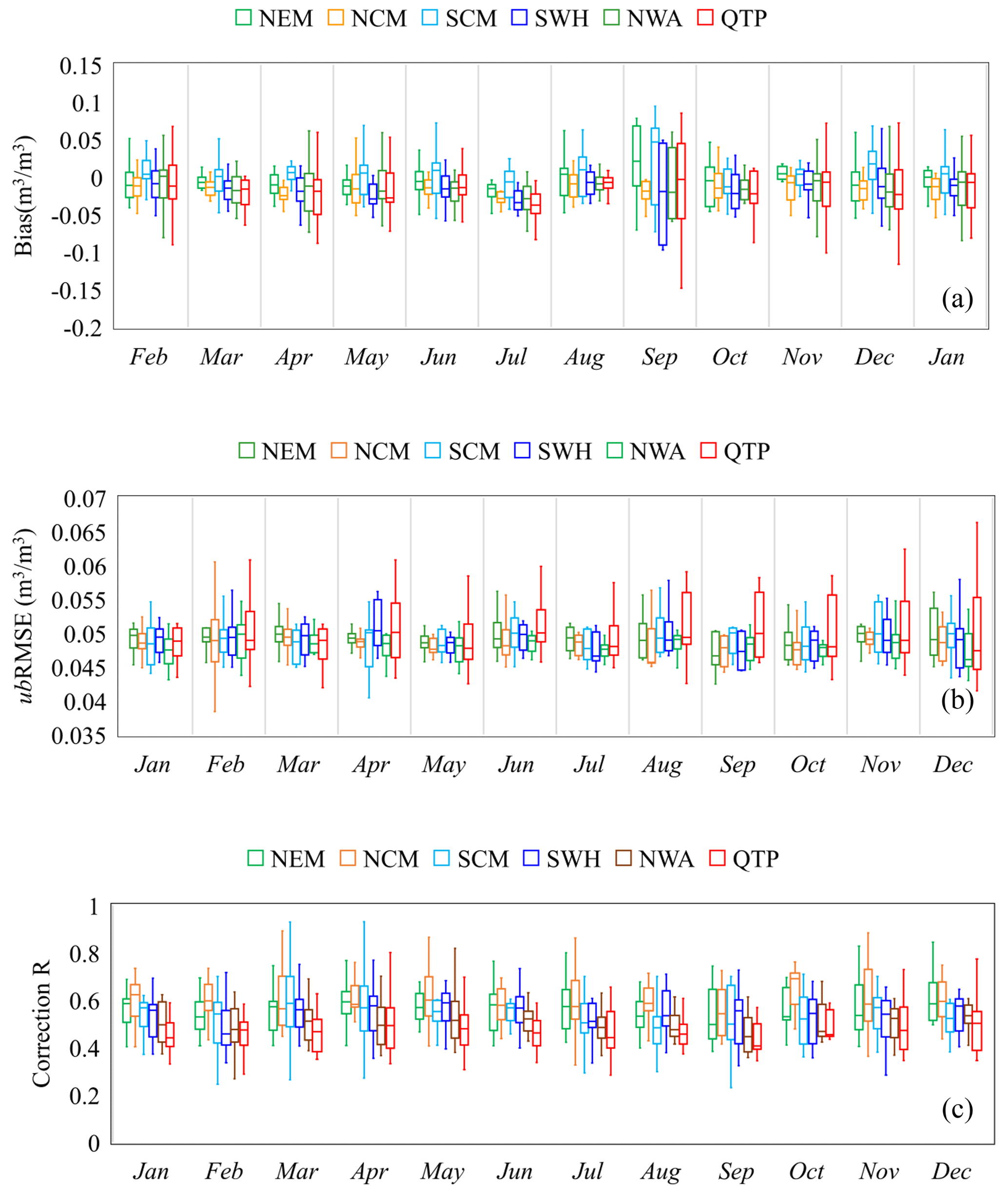
Figure 4Box plots of the RMSE, bias and R (p <0.05) of comparison between downscaled SM and in situ SM in each region.
Although the downscaled SM products generally show higher accuracy, we still further analyzed the consistency of the downscaled SM and the ground-measured SM in different regions. In Fig. 4, the box plots present the median for each indicator (the horizontal line within each box) and the first (Q1) and third quantiles (represented by the bottom and top of the box, respectively). The downscaled SM is strongly correlated with the in situ measurements, with mean R > 0.64 during 12 months in the subregions. Specifically, the downscaled SM products have the lowest R and the highest bias and ubRMSE in December. The downscaled SM products display the best correlation with in situ measurements in September (weaker vegetation impact). Compared to the values in the North China Monsoon and Northeast Monsoon regions, the deviation values in the South China Monsoon and the Qinghai–Tibet Plateau regions are more variable. The reasons for this variability are different. Some areas of the Qinghai–Tibet Plateau are covered by snow and ice all year round or in some seasons, while some regions in southern China have relatively more rainfall in some seasons. We need to know that the errors of SM data in these areas, especially in frozen soil areas, are relatively large. To maintain the integrity of the data, we retain these data because a previous study demonstrated that the JAXA AMSR-E and AMSR2 products still have some ability to capture the temporal trend of SM in frozen seasons (Zeng et al., 2015). Therefore, the follow-up verification and analysis process also follows this criterion.
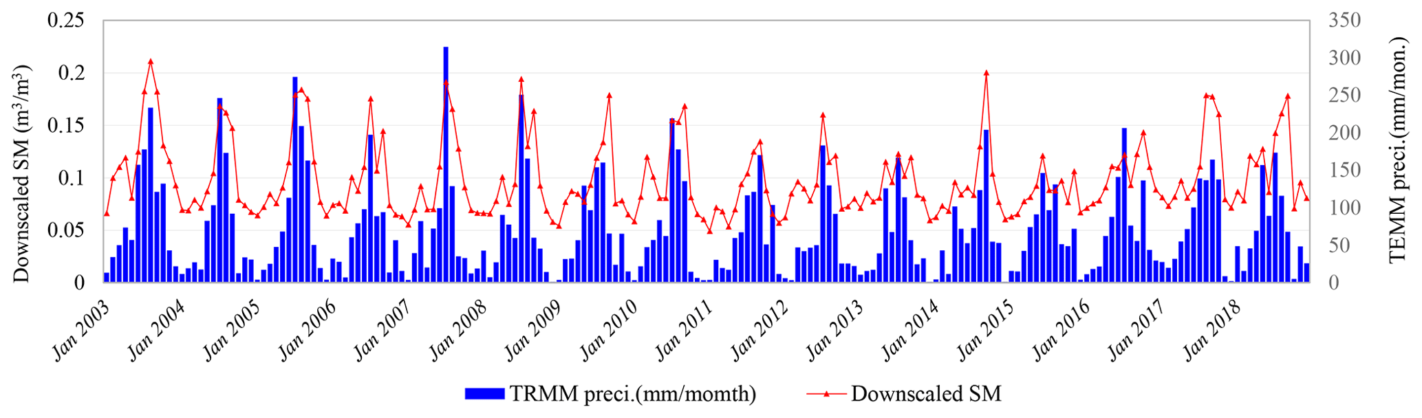
Figure 5Time series of the area mean downscaled SM and TRMM precipitation during the study period from 2003 to 2018.
In addition, due to the high correlation between soil moisture and precipitation changes, we also explored downscaling time series of SM and TRMM precipitation. The analysis in Fig. 5 shows that the SM products after downscaling are highly consistent with changes in rainfall. Overall, the above results further demonstrate the effectiveness of the downscaled SM, which means that the downscaled SM value is suitable for high-precision hydrology and drought monitoring applications.
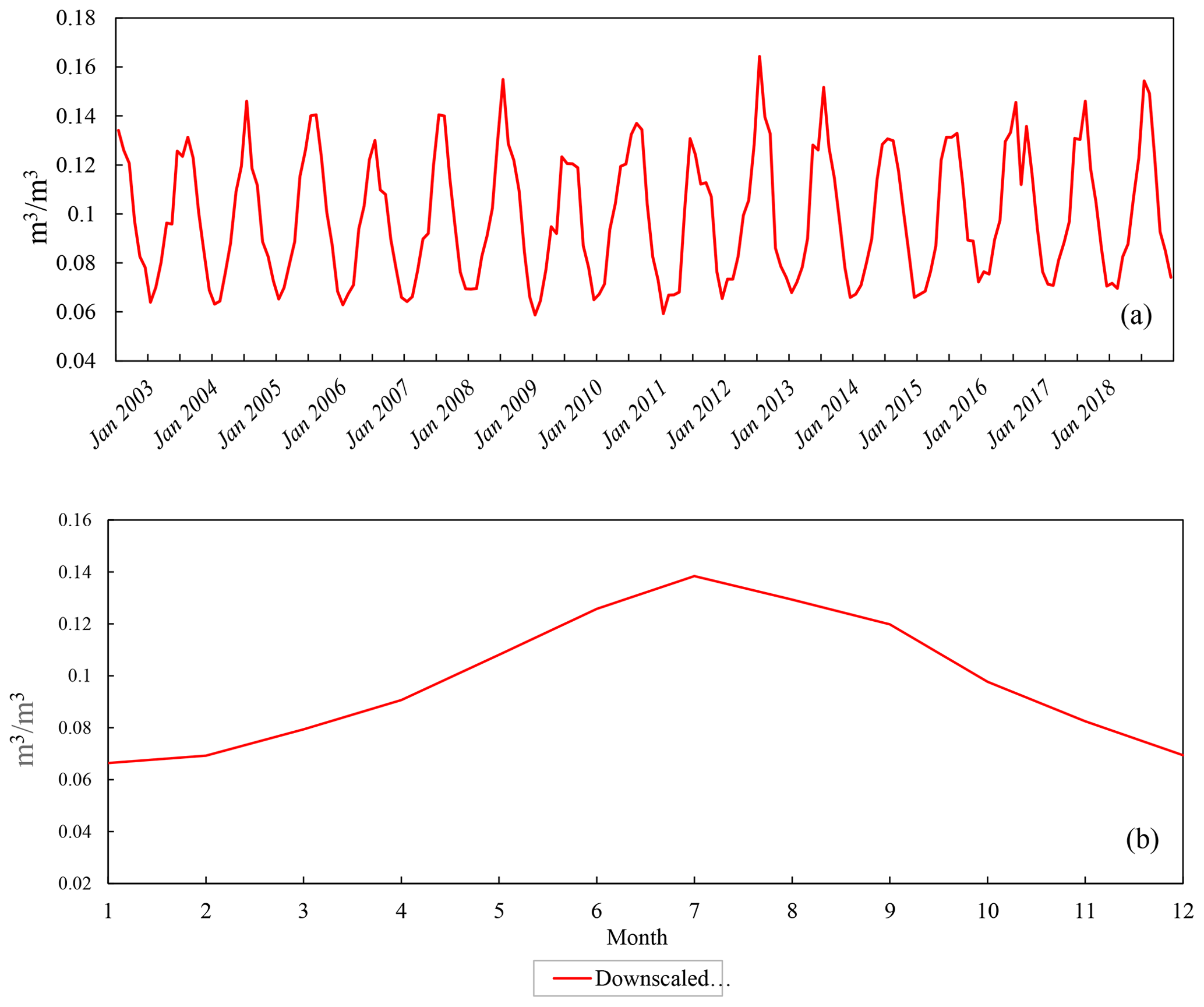
Figure 6Time series of the area mean downscaled SM during the study period from June 2002 to December 2018.
4.2 Spatiotemporal changes in SM in different natural regions of China
Figure 6a shows that downscaled SM can represent the typical seasonal variations well, with minimum SM in winter and maximum SM in summer affected by the monsoon in China. The figure also illustrates that the downscaled SM captures the extreme drought events occurring in 2009, 2011 and 2015 well.
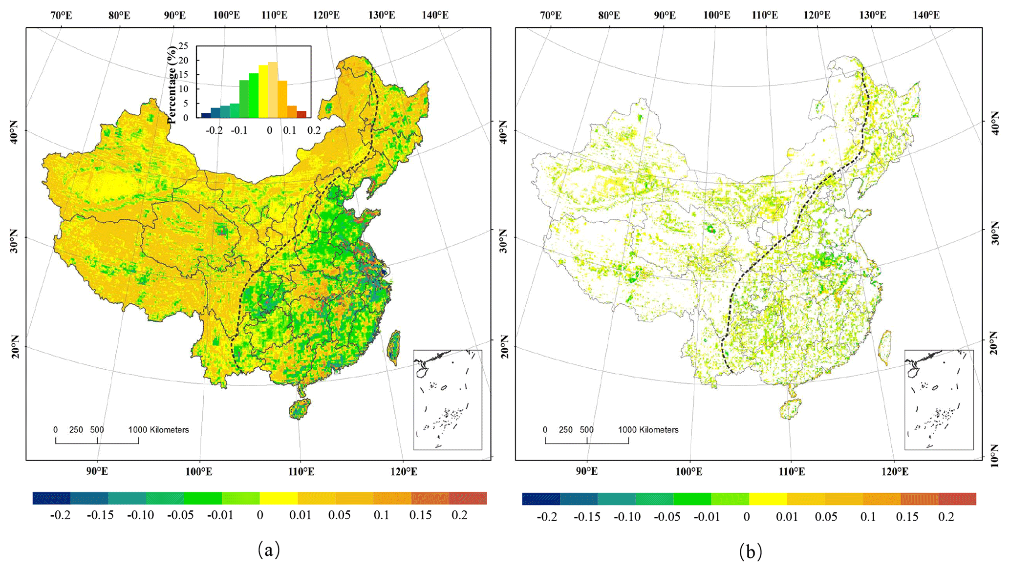
Figure 7Spatial distribution of annual SM variability in slope based on downscaled data from 2002 to 2018. (a) Slope trend values of all pixels and (b) propensity slope trend values is at 90 % confidence level. The dotted black line is the dividing line between wet and dry changes.
4.3 Characteristics of the spatiotemporal variations in SM
In order to obtain the long-term changes in the spatial details of the downscaled surface SM, a linear regression slope was performed at the pixel level from 2002 to 2018. The slope is used to represent the variation rate of the downscaled SM. If the slope value is greater than 0, SM has become wetter and wetter in the past 17 years, with a higher value indicating a more pronounced change. When the slope value is less than 0, the surface soil water has tended to become dry in the past 17 years with a higher negative value indicating a more pronounced change, and a slope = 0 indicates no change. Figure 7a is a map of the spatial trend change (slope) of SM, and Fig. 7b is propensity slope trend values at 90 % confidence level.
On the whole, most areas in northwestern China tend to become slightly wetter, while some parts of the eastern region become drier and some parts become slightly wetter. This result also just verified the view that people have been discussing, which is the gradual wetness of northwestern China in recent years (Cong et al., 2017). We think that the main reason is that global warming has promoted the intensification of the water cycle, which is the main cause of climate warming and humidification in the northwest. For the northwest region, water vapor mainly comes from the Arabian Sea and the Indian Ocean. As the Arctic warms, water vapor from the Arctic Ocean increases. Under the influence of air currents, the water vapor of the three places concentrated in the northwest of China, and the precipitation increased rapidly, resulting in an increase in soil moisture. In the eastern monsoon region, including a small part of Inner Mongolia, the junction of Jilin and Liaoning, the North China Plain, southern Shaanxi, eastern Shanxi, and most parts of Henan, Hebei and Shandong, there is a tendency to become drier, which has been reported in some studies (Liang et al., 2017). Especially in the Huai River Basin (north of SCM), that is the SCM including Jiangsu and Zhejiang, there is a trend of drying up. In southern Guangdong, the mountainous areas of Fujian and parts of Jiangxi show a trend of getting wetter. In SWH, the Sichuan Basin is expected to become drier, and the Yunnan–Guizhou Plateau is also facing a relatively dry situation. The main reason for this phenomenon is that during this period, the southwestern region experienced high temperatures leading to a large amount of evaporation which caused the soil moisture to decrease. This result indicates that the agricultural drought risk in SWH will increase in the future. As shown in Fig. 7b, the distribution of significant dryness changes (satisfying the 90 % confidence interval) is relatively scattered, accounting for about 13 % of the total pixels, mainly distributed in Horqin Sandy Land (northeast of NWA), North China Plain, Henan, Jiangsu–Zhejiang region, eastern Tibet and other places. The significant wetness area is about 10 % of the total pixels, mainly distributed in northwestern Qinghai and eastern Xinjiang. The main areas that become drier and wetter are basically consistent with the boundary between the first and second steps of elevation in Fig. 1 and the Hu's line (the dotted black line in Fig. 7). This is an interesting phenomenon which means that precipitation and topography affect not only the spatial distribution of soil moisture but also the change in SM.
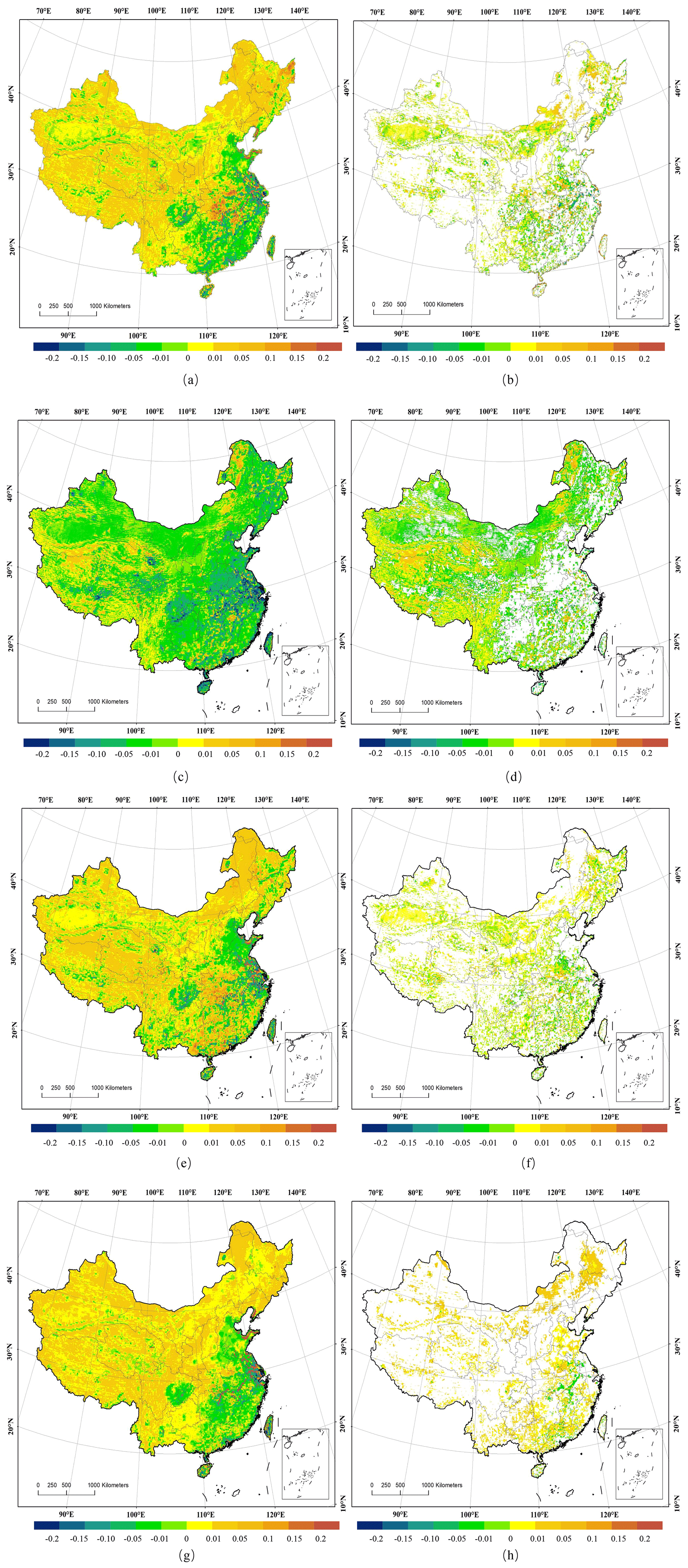
Figure 8The interannual variability rates (slopes) and correlation coefficients (R) of the seasonal average SM from 2002 to 2018, for which (a), (c), (e) and (g) are the changing trends of all pixels in spring, summer, autumn and winter, respectively, and for which (b), (d), (f) and (h) are the changing trends of pixels satisfying 90 % confidence in spring, summer, autumn and winter, respectively.
To better understand the SM changes throughout China, the spatial distributions of the annual variations in the SM for different regions in different seasons are analyzed. Figure 8 shows the pixel-level trend of SM data in each season. We found that the changes in soil moisture in spring (Fig. 8a) and autumn (Fig. 8c) are generally similar to the annual trend, while the soil moisture in most areas tends to become drier in summer (Fig. 8b). Soil moisture except for a few areas in southeast China becomes drier, while most areas of China become wetter in winter (Fig. 8d).
In the spring and autumn seasons, the line of dry and wet changes is distributed from the east to the west. The overall situation is that the east becomes drier and the west becomes wetter. The difference is that the Sichuan Basin becomes drier and the middle reaches of the Yangtze River wetter. Generally, due to the large changes in the interannual hydrothermal and monsoon precipitation, the area affected by the monsoon in the east varied greatly. From spring to summer, the range of fluctuation of SM in the South China Monsoon Region was significantly enhanced. Usually, shifts in precipitation belts occur during the rainy season. These shifts are governed by the summer monsoon and occur during the rainy season in the Pearl River Delta and Yangtze River Delta (Zhou et al., 2010). During the rainy season, the total rainfall was approximately 80 % of the annual rainfall (Yan et al., 2015). However, in summer, there are more pixels becoming drier than becoming wetter, which means the vegetation is vulnerable to drought during the main growing season. In summer and autumn, the trends in the monsoon regions are obvious. Although many rainfall events occur in the summer and autumn monsoon regions, the spatial and temporal distributions of precipitation were not balanced. In addition, the middle and lower reaches of the Yangtze River are mainly dominated by a subtropical high-pressure system in summer during which a large amount of evaporation takes place, which may have been the main cause of the observed decline. The change in SM in winter was not as significant as that in other seasons. Conversely, the SM increased in areas affected by monsoons, such as the Qinghai–Tibet Plateau Region (southern Tibet) and the Northwest Arid Region (eastern Inner Mongolia).
The code for the reconstruction model-based downscaling techniques can be downloaded at https://doi.org/10.5281/zenodo.4922393 (Meng et al., 2021b).
The fine-resolution surface soil moisture (SSM) dataset presented in this article is available under the Creative Commons Attribution 4.0 International License at the following link: https://doi.org/10.5281/zenodo.4738556 (Meng et al., 2021a). This dataset covers all of China's land area at a monthly temporal resolution and a 0.05∘ spatial resolution from July 2002 to December 2018.
Although there are many soil moisture algorithms and products, different algorithms have their own advantages and disadvantages, and their accuracy performance is inconsistent in different regions. The main reason is that the resolution of passive microwave is too low, and the theoretical model of large-scale (mixed) pixels is not very mature. Deep learning algorithms have certain advantages, but their accuracy depends on training and test data. Especially in areas with a lot of vegetation and rainfall, the accuracy performance is inconsistent for different algorithms. For example, in vegetation coverage areas, single albedo and optical thickness coefficient values are obtained differently for different retrieval algorithms, which results in some difference in soil moisture retrieval. Another difference is the treatment of heavy rainfall. When there is heavy rainfall, the soil moisture error retrieved by microwave remote sensing is also very large. Some retrieval algorithms determine that when there is heavy rainfall, the retrieval soil moisture is an invalid value or a null value, but some algorithms directly set the soil moisture saturation value as the soil moisture value. We need to overcome the above problems as much as possible and improve the accuracy of data products based on the observation data of SM at the site.
The global soil moisture dataset is constantly being produced; especially in recent years, the frequency of updates is getting faster and faster. Each soil moisture dataset and method of producing SM has its own advantages and disadvantages. Our SM dataset is mainly concentrated in China. Two similar sensors mounted on different satellites are used to produce a set of SM datasets that are continuous in time and space in China. For the missing part between AMSR-E and AMSR2 sensors, a relatively reliable sensor was used to make up for it. In order to ensure the consistency of the time and depth of the observation data of the three instruments, we have made corrections through building the reconstruction model. In particular, we took advantage of ground observation site data to make local improvements. To meet the needs of research such as agricultural drought monitoring, we downscaled the soil moisture products and obtained a higher-resolution dataset.
Based on the inversion of soil moisture products using microwave sensors mounted on three different satellites, two models were established to eliminate the difference between observation time and observation depth, and a time-continuous soil moisture dataset was generated for the period from 2002 to 2018. In order to further meet the needs of local monitoring and research, a downscaling model was constructed using visible light and thermal infrared data, and then the soil moisture dataset was downscaled to generate a set of soil moisture datasets with a spatial resolution of 0.05∘. A detailed comparison and analysis with the in situ measurements show that the reconstruction results have high precision, and the biases are −0.057, −0.063 and −0.027 m3 m−3, unbiased root mean square errors (ubRMSEs) are 0.056, 0.036 and 0.048 m3 m−3, and correlation coefficients (R) are 0.84, 0.85 and 0.89 on monthly, seasonal and annual scales, respectively. The data are freely available at https://doi.org/10.5281/zenodo.4738556 (Meng et al., 2021a). In order to cross-validate with the low-resolution soil moisture dataset (RSSSM data; Chen et al., 2021), we upscaled the soil moisture dataset and then did a cross-validation analysis. The analysis results in Appendix B show that the two datasets have a high consistency in time and space, which indirectly shows that our soil moisture dataset is reliable. The change in soil moisture is also affected by rainfall, and we further analyzed the relationship between the temporal and spatial changes in soil moisture and precipitation, showing that there is a high consistency between them.
The high-spatial-resolution monthly SM dataset constructed for China provides a detailed perspective of the patterns of the spatial and temporal changes in SM. The SM dataset was used to analyze the regional characteristics and capture the variations in SM at the annual, seasonal and monthly scales. The results showed that the soil moisture in China has been shown to generally exhibit cyclical fluctuations, which can be summarized as a slight downward trend in the southeast and a slight upward trend in the northwest. Most areas have a drying trend in summer, while most areas have the opposite in autumn. The main reason for soil moisture variation in northwestern China may be that global warming drives the intensification of the water cycle, which is the fundamental reason for the warming and humidification of the climate in northwestern China. For the northwest, water vapor mainly comes from the Arabian Sea and the Indian Ocean. As the Arctic warms, water vapor from the Arctic Ocean increases. Under the action of air currents, water vapor in the three places concentrated in the northwest, and precipitation in the northwest increased rapidly, which leads to an increase in soil moisture. The dryness of southeastern China is mainly due to the increase in evaporation caused by the increase in temperature, which leads to the decrease in soil moisture. Of course, it may also be affected by more factors, such as El Niño and La Niña, which requires further research in the future.
Due to the influence of large-scale mixed pixels and rainfall, the soil moisture retrieval algorithm has been continuously improved, and the corresponding soil moisture datasets are also constantly updated. In the past 2 years, we have updated three versions of soil moisture datasets. In order to promote research in agricultural drought monitoring and weather forecasting, we will continue to update more high-precision soil moisture products in the future.
A1 In situ SM measuring stations
The SM data are provided by China's national meteorological stations (CNMSs) and China's agrometeorological and ecological observation network (shown in Fig. A1), and the measured value is relative soil humidity (%). The shallowest observation depth of the site is 10 cm to match the surface SM. The remote sensing inversion data are expressed in volumetric water content (m3 m−3). Before comparison and verification, it is necessary to convert different units, and the formula (A1) can be used to convert the relative humidity of the site SM to the soil volumetric water content.
where VSM is the soil volumetric water content (%), Mv is the relative humidity of the soil, V is the field water holding capacity, and ρs is the soil density.
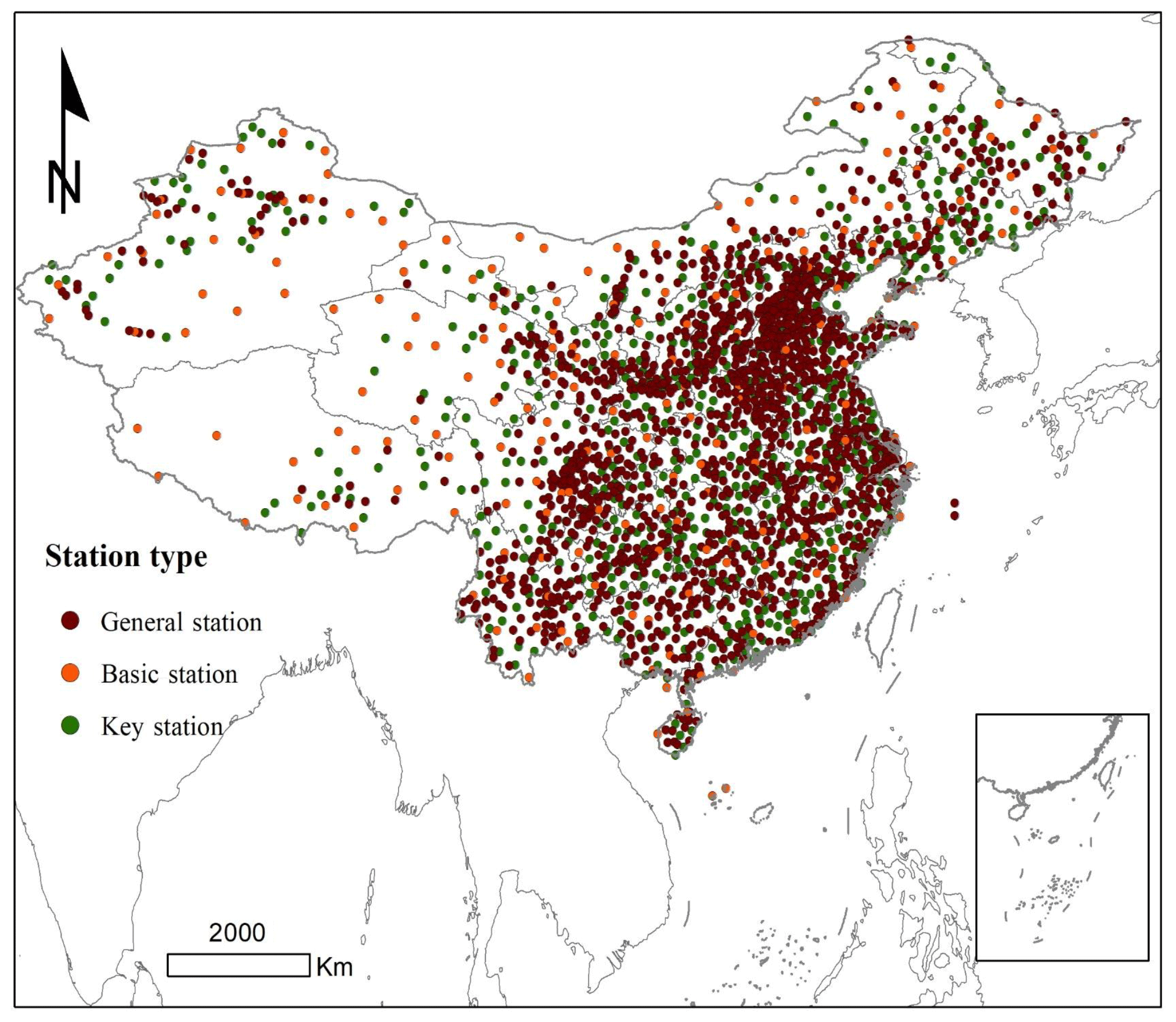
Figure A1Distribution of China's national meteorological stations (CNMSs) and China's agrometeorological and ecological observation network stations (general station, basic station and key station).
A2 Downscaled results
Figure A2 display the original and downscaled fine-resolution SM products of China, and it can be seen that the downscaled SM can present much more spatial details compared with the original SM product.
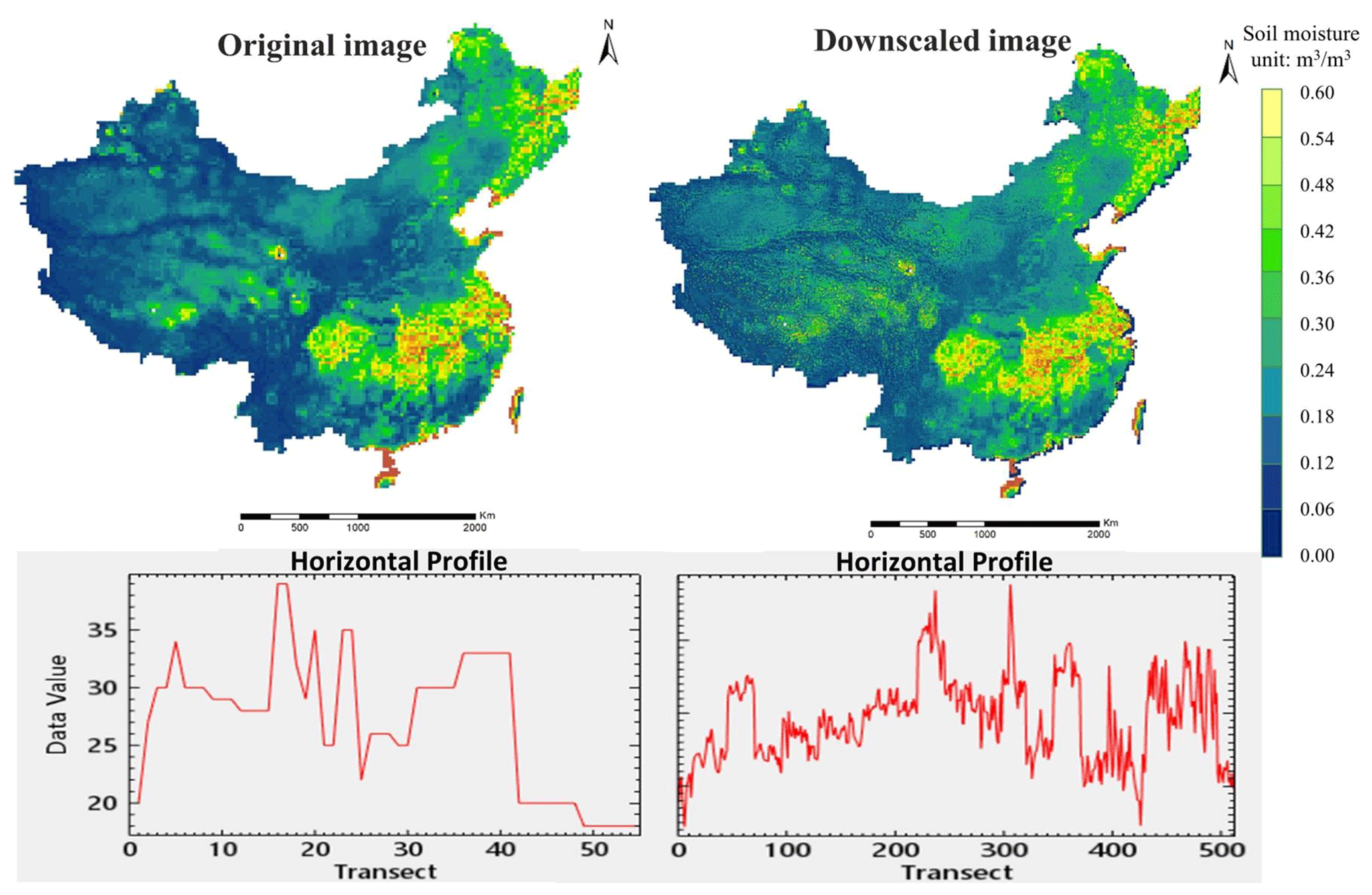
Figure A2Comparison of downscaled SM images and original images.
Scatterplots of RSSSM with downscaled SM in the six subregions are shown in Fig. B1. In general, good agreements between RSSSM and downscaled SM products can be found in the six subregions. It can also be observed that the overall value of downscaling products is lower compared with RSSSM. The depth represented by the soil moisture inverted by different data sources is inconsistent, resulting in different moisture values, which are similar to results of JAXA production reported by published studies (Zeng et al., 2015; Cui et al., 2018).

KM and FM designed the research and developed the methodology; KM and XM supervised the downloading and processing of satellite images; XM wrote the manuscript; and JS, JZ, XS, YC, LJ, ZG and all other authors revised the manuscript.
The authors declare that they have no conflict of interest.
Publisher's note: Copernicus Publications remains neutral with regard to jurisdictional claims in published maps and institutional affiliations.
The authors thank the China Meteorological Administration for providing the ground measurements, the Japan Aerospace Exploration Agency for providing the AMSR-E and AMSR2 SM data, the ESA Earth Observation User Services Portal of the European Aviation Administration for providing the SMOS-IC SM data, and the NASA Earth Observing System Data and Information System for providing the MODIS LST and NDVI data and DEM data.
This work was supported by the Second Tibetan Plateau Scientific Expedition and Research Program (STEP) “Dynamic monitoring and simulation of water cycle in Asian water tower area” (grant no. 2019QZKK0206), the National Key Project of China (grant no. 2018YFC1506602), the National Natural Science Foundation of China (grant no. 41921001), the Fundamental Research Funds for Central Nonprofit Scientific Institution (grant no. 1610132020014) and the Open Fund of the State Key Laboratory of Remote Sensing Science (grant no. OFSLRSS201910).
This paper was edited by Prasad Gogineni and reviewed by two anonymous referees.
Afshar, M. and Yilmaz, M.: The added utility of nonlinear methods compared to linear methods in rescaling soil moisture products, Remote Sens. Environ., 196, 224–23, https://doi.org/10.1016/j.rse.2017.05.017, 2017.
Albergel, C., Rosnay, P. D., Gruhier, C., Muño-Sabater, J. S., Hasenauer, S., Isaksen, L., Kerr, Y., and Wagner. W.: Evaluation of remotely sensed and modelled soil moisture products using global ground-based in situ observations, Remote Sens. Environ., 118, 215–226, https://doi.org/10.1016/j.rse.2011.11.017, 2012.
Albergel, C., Dorigo, W., Balsamo, G., Muñoz-Sabatera, J., de Rosnay, P., Isaksen, L., and Wagner, W.: Monitoring multi-decadal satellite earth observation of soil moisture products through land surface reanalyses, Remote Sens. Environ., 138, 77–89, https://doi.org/10.1016/j.rse.2013.07.009, 2013.
Al-Yaari, A., Wigneron J. P., Dorigo, W., Colliander, A., Pellarin, T., Hahn, S., Mialon, A., Richaume, P., Fernandez-Moran, R., Fan, L., Kerr, Y., and Lannoy, G.: Assessment and inter-comparison of recently developed/reprocessed microwave satellite soil moisture products using ISMN ground-based measurements, Remote Sens. Environ., 224, 289–303, https://doi.org/10.1016/j.rse.2019.02.008, 2019.
Bhagat, S. V.: Space-borne passive microwave remote sensing of soil moisture: A review, Recent Patents on Space Technology, 4, 119–150, https://doi.org/10.2174/221068710402150513123146#sthash.qA8fxZDt.dpuf, 2014.
Bindlish, R., Crow, W. T., and Jackson, T. J.: Role of passive microwave remote sensing in improving flood forecasts, IEEE Geosci. Remote S., 1, 112–116, https://doi.org/10.1109/LGRS.2008.2002754, 2009.
Brocca, L., Melone, F., Moramarco, T., Wagner, W., and Albergel, C.: Scaling and filtering approaches for the use of satellite soil moisture observations, in: Remote Sensing of Energy Fluxes and Soil Moisture Content, edited by: Petropoulos, G., Boca Raton, 411–426, ISBN:978-1-4665-0578-0, 2013.
Carlson, T. N., Gillies, R. R., and Perry, E. M.: A method to make use of thermal infrared temperature and NDVI measurements to infer surface soil water content and fractional vegetation cover, Remote Sens. Reviews, 9, 161–173, https://doi.org/10.1080/02757259409532220, 1994.
Cashion, J., Lakshmi, V., Bosch, D., and Jackson, T. J.: Microwave remote sensing of soil moisture: Evaluation of the TRMM microwave imager (TMI) satellite for the Little River Watershed Tifton, J. Hydrol., 307, 242–253, https://doi.org/10.1016/j.jhydrol.2004.10.019, 2005.
Chauhan, N. S., Miller, S., and Ardanuy, P.: Space bore soil moisture estimation at high resolution: a microwave-optical/IR synergistic approach, Int. J. Remote Sens., 22, 4599–4622, https://doi.org/10.1080/0143116031000156837, 2003.
Chen, C. F., Son, N. T., Chang, L. Y., and Chen, C. C.: Monitoring of soil moisture variability in relation to rice cropping systems in the Vietnamese Mekong Delta using MODIS data, Appl. Geogr., 2, 463–475, https://doi.org/10.1016/j.apgeog.2010.10.002, 2011.
Chen, Y., Feng, X., and Fu, B.: An improved global remote-sensing-based surface soil moisture (RSSSM) dataset covering 2003–2018, Earth Syst. Sci. Data, 13, 1–31, https://doi.org/10.5194/essd-13-1-2021, 2021.
Choi, M. and Hur, Y.: A microwave-optical/infrared disaggregation for improving spatial representation of soil moisture using AMSR-E and MODIS products, Remote Sens. Environ., 124, 259–269, https://doi.org/10.1016/j.rse.2012.05.009, 2012.
Cong, D., Zhao, S., Chen, C., and Duan, Z.: Characterization of droughts during 2001-2014 based on remote sensing: a case study of Northeast China, Ecol. Inform., 39, 56–67, https://doi.org/10.1016/j.ecoinf.2017.03.005, 2017.
Crow, W. T. and Zhan, X.: Continental-scale evaluation of remotely sensed soil moisture products, IEEE Geosci. Remote S., 3, 451–455, https://doi.org/10.1109/LGRS.2007.896533, 2007.
Crow, W. T., Berg, A. A., Cosh, M. H., Loew, A., Mohanty, B. P., Panciera, R., Rosnay, P., Ryu, D., and Walker, J. P.: Upscaling sparse ground-based soil moisture observations for the validation of coarse-resolution satellite soil moisture products, Rev. Geophys., 50, 1–20, https://doi.org/10.1029/2011RG000372, 2002.
Cui, C. Y., Xu, J., Zeng, J. Y., Chen, K. S., Bai, X. J., Lu, H., Chen, Q., and Zhao, T. J.: Soil moisture mapping from satellites: an intercomparison of SMAP, SMOS, FY3B, AMSR2, and ESA CCI over two dense network regions at different spatial scales, Remote Sens.-Basel, 33, 1–19, https://doi.org/10.3390/rs10010033, 2018.
Dorigo, W., Gruber, A., De Jeu, R., Wagner, W., Stacke, T., Loew, A., Albergel, C., Brocca, L., Chung, D., Parinussa, R., and Kidd, R.: Evaluation of the ESA CCI soil moisture product using ground-based observations, Remote Sens. Environ., 162, 380–395, https://doi.org/10.1016/j.rse.2014.07.023, 2015.
Dorigo, W., Wagner, W., Albergel, C., Albrecht, F., Balsamo, G., Brocca, L., Chung, D., Ertl, M., Forkel, M., Gruber, A., Haas, E., Hamer, D. P. Hirschi, M., Ikonen, J., De Jeu, R. Kidd, R. Lahoz, W., Liu, Y., Miralles, D., and Lecomte, P.: ESA CCI Soil Moisture for improved Earth system understanding: State-of-the art and future directions, Remote Sens. Environ., 15, 185–215, https://doi.org/10.1016/j.rse.2017.07.001, 2017.
Dorigo, W. A., Wagner, W., Hohensinn, R., Hahn, S., Paulik, C., Xaver, A., Gruber, A., Drusch, M., Mecklenburg, S., van Oevelen, P., Robock, A., and Jackson, T.: The International Soil Moisture Network: a data hosting facility for global in situ soil moisture measurements, Hydrol. Earth Syst. Sci., 15, 1675–1698, https://doi.org/10.5194/hess-15-1675-2011, 2011.
Draper, C. S., Walker, J. P., and Steinle, P. J.: An evaluation of AMSR-E derived soil moisture over Australia, Remote Sens. Environ., 4, 703–710, https://doi.org/10.1016/j.rse.2008.11.011, 2009.
Fernandez-Moran, R., Al-Yaari, A. A., Mialon, A., Mahmoodi, A., Al Bitar, G., De Lannoy, N., Rodriguez-Fernandez, E., Lopez-Baeza, Y., Kerr, and Wigneron, J. P.: SMOS-IC: An alternative SMOS soil moisture and vegetation optical depth product, Remote Sens.-Basel, 9, 1–21, https://doi.org/10.3390/rs9050457, 2017.
Franz, T. E., Zreda, M., Rosolem, R., and Ferre, T. P. A.: A universal calibration function for determination of soil moisture with cosmic-ray neutrons, Hydrol. Earth Syst. Sci., 17, 453–460, https://doi.org/10.5194/hess-17-453-2013, 2013.
González-Zamora, A., Sánchez, N., Martínez-Fernández, J., Gumuzzio, A., Piles, M., and Olmedo, E.: Long-term SMOS soil moisture products: A comprehensive evaluation across scales and methods in the Duero Basin (Spain), Phys. Chem. Earth, 83–84, 123–136, https://doi.org/10.1016/j.pce.2015.05.009, 2015.
Gruber, A., Scanlon, T., van der Schalie, R., Wagner, W., and Dorigo, W.: Evolution of the ESA CCI Soil Moisture climate data records and their underlying merging methodology, Earth Syst. Sci. Data, 11, 717–739, https://doi.org/10.5194/essd-11-717-2019, 2019.
Guillod, B. P., Orlowsky, B., Miralles, D. G., Teuling, A. J., and Seneviratne, S. I.: Reconciling spatial and temporal soil moisture effects on afternoon rainfall, Nat. Commun., 6, 1–6, https://doi.org/10.1038/ncomms7443, 2015.
Han, E., Merwade, V., and Heathman, G. C.: Implementation of surface soil moisture data assimilation with watershed scale distributed hydrological model, J. Hydrol., 416–417, 98–117, https://doi.org/10.1016/j.jhydrol.2011.11.039, 2012.
Im, J., Park, S., Rhee, J., Baik, J., and Choi, M.: Downscaling of AMSR-E soil moisture with MODIS products using machine learning approaches, Environ. Earth Sci., 15, 1120, 1–19, https://doi.org/10.1007/s12665-016-5917-6, 2016.
Jin, Y., Ge, Y., Wang, J., Chen, Y., Heuvelink, G. B. M., and Atkinson, P. M.: Downscaling AMSR-2 soil moisture data with Geographically weighted area-to-area regression kriging, IEEE T. Geosci. Remote, 56, 2362–2376, https://doi.org/10.1109/TGRS.2017.2778420, 2017.
Jing, W., Zhang, P., and Zhao, X.: Reconstructing monthly ECV global soil moisture with an improved spatial resolution, Water Resour. Manag., 32, 1–21, https://doi.org/10.1007/s11269-018-1944-2, 2018.
Kang, C. S., Zhao, T., Shi, J., Cosh, M. H., Chen, Y., Starks, P. J., Collins, C. H., Wu, S., Sun, R., and Zheng, J.: Global soil moisture retrievals from the Chinese FY-3D microwave radiation imager, IEEE T. Geosci. Remote, 5, 4018–4032, https://doi.org/10.1109/TGRS.2020.3019408, 2020.
Kerr, Y. H., Waldteufel, P., Richaume, P., Wigneron, J. P., Ferrazzoli, P., Mahmoodi, A., Bitar, A. A., Cabot, F., Gruhier, C., Juglea, S. E., Leroux, D., Moalon, A., and Delwart, S.: The SMOS soil moisture retrieval algorithm, IEEE T. Geosci. Remote, 5, 1384–1403, https://doi.org/10.1109/TGRS.2012.2184548, 2012.
Kim, J. and Hogue, T. S.: Improving spatial soil moisture representation through integration of AMSR-E and MODIS products, IEEE T. Geosci. Remote, 2, 446–460, https://doi.org/10.1109/TGRS.2011.2161318, 2012.
Kim, S., Liu, Y. Y., Johnson, F. M., Parinussa, R. M., and Sharma, A.: A global comparison of alternate AMSR2 soil moisture products: Why do they differ?, Remote Sens. Environ., 61, 43–62, https://doi.org/10.1016/j.rse.2015.02.002, 2015.
Koike, T., Nakamura, Y., Kaihotsu, I., Davva, G., Matsuura, N., Tamagawa, K., and Fujii, H.: Development of an advanced microwave scanning radiometer (AMSR-E) algorithm of soil moisture and vegetation water content, Proceedings of Hydraulic Engineering, 48, 217–222, https://doi.org/10.2208/prohe.48.217, 2004.
Lacava, T., Matgen, P., Brocca, L., Bittelli, M., Pergola, N., Moramarco, T., and Tramutoli, V.: A first assessment of the SMOS soil moisture product with in situ and modeled data in Italy and Luxembourg, IEEE T. Geosci. Remote, 5, 1612–1622, https://doi.org/10.1109/TGRS.2012.2186819, 2012.
Liang, L., Sun, Q., Luo, X., Wang, J., Zhang, L., Deng, M., Di, L., and Liu, Z.: Long-term spatial and temporal variations of vegetative drought based on vegetation condition index in China, Ecosphere, 8, 1–15, https://doi.org/10.1002/ecs2.1919, 2017.
Liu, L., Liao, J., Chen, X., Zhou, G., and Shao, H.: The microwave temperature vegetation drought index (MTVDI) based on AMSR-E brightness temperatures for long-term drought assessment across China (2003–2010). Remote Sens. Environ., 199, 302–320, https://doi.org/10.1016/j.rse.2017.07.012, 2017.
Liu, Y. Y., van Dijk, A. I. J. M. V., de Jeu, R. A. M., and Holmes, T. R. H.: An analysis of spatiotemporal variations of soil and vegetation moisture from a 29-year satellite-derived data set over mainland Australia, Water Resour. Res., 7, 4542–4548, https://doi.org/10.1029/2008WR007187, 2009.
Liu, Y. Y., Parinussa, R. M., Dorigo, W. A., De Jeu, R. A. M., Wagner, W., van Dijk, A. I. J. M., McCabe, M. F., and Evans, J. P.: Developing an improved soil moisture dataset by blending passive and active microwave satellite-based retrievals, Hydrol. Earth Syst. Sci., 15, 425–436, https://doi.org/10.5194/hess-15-425-2011, 2011.
Liu, Y. Y., Dorigo, W. A., Parinussa, R. M., de Jeu, R. A. M., Wager, W., McCabe, M. F., Evans, J. P., and van Dijik, A. I. J. M.: Trend-preserving blending of passive and active microwave soil moisture retrievals, Remote Sens. Environ., 123, 280—297, https://doi.org/10.1016/j.rse.2012.03.014, 2012.
Loew, A. and Schlenz, F.: A dynamic approach for evaluating coarse scale satellite soil moisture products, Hydrol. Earth Syst. Sci., 15, 75–90, https://doi.org/10.5194/hess-15-75-2011, 2011.
Loew, A., Stacke, T., Dorigo, W., de Jeu, R., and Hagemann, S.: Potential and limitations of multidecadal satellite soil moisture observations for selected climate model evaluation studies, Hydrol. Earth Syst. Sci., 17, 3523–3542, https://doi.org/10.5194/hess-17-3523-2013, 2013.
Ma, H., Zeng J., Chen, N., Zhang, X., Cosh, M. H., and Wang,W.: Satellite surface soil moisture from SMAP, SMOS, AMSR2 and ESA CCI: A comprehensive assessment using global ground-based observations. Remote Sens. Environ., 231, 1–14, https://doi.org/10.1016/j.rse.2019.111215, 2019.
Maltese, A., Capodici, F., Ciraolo, G., and La Loggia, G.: Soil water content assessment: Critical issues concerning the operational application of the triangle method, Sensors, 3, 6699–6718, https://doi.org/10.3390/s150306699, 2015.
Mao, K. B., Tang H. J., Zhang, L. X., Li, M. C., Y., and Zhao, D. Z.: A method for retrieving soil moisture in Tibet region by utilizing microwave index from TRMM/TMI data, Int. J. Remote Sens., 10, 2905–2925, https://doi.org/10.1080/01431160701442104, 2008a.
Mao, K. B, Shi, J. C., Tang, H., Li, Z. L., Wang, X., and Chen, K. S.: A neural network technique for separating land surface emissivity and temperature from aster imagery, IEEE T. Geosci. Remote, 1, 200–208, https://doi.org/10.1109/TGRS.2007.907333, 2008b.
Mao, K. B., Gao, C. Y., Han, L. J., and Zhang, W.: The drought monitoring in China by using AMSR-E data, 2010 Sec. IITA Inter. Confer. on Geosci. and Remote Sens., Qingdao, China, 28–31 August 2010, 181–184, https://doi.org/10.1109/IITA-GRS.2010.5603008, 2010.
Mao, K. B., Ma, Y., Xia, L., Tang, H. J., and Han, L, J.: The monitoring analysis for the drought in China by using an improved MPI method, J. Integr. Agr., 6, 1048–1058, https://doi.org/10.1016/S2095-3119(12)60097-5, 2012,.
Meng, X., Mao, K., Meng, F., Shi, J., Zeng, J., Shen, X., Cui, Y., Liang, L., and Guo, Z.: A fine-resolution soil moisture dataset for China in 2002 ∼ 2018 (Version 3.0) [Data set], Zenodo, https://doi.org/10.5281/zenodo.4738556, 2021a.
Meng, X., Mao, K., Meng, F., Shi, J., Zeng, J., Shen, X., Cui, Y., Liang, L., and Guo, Z.: A fine-resolution soil moisture dataset for China in 2002 ∼ 2018 (Version 3.0) [Code], Zenodo, https://doi.org/10.5281/zenodo.4922393, 2021b.
Mohanty, B., Cosh, M., Lakshmi, V., and Montzka, C.: Soil moisture remote sensing: state-of-the-science, Vadose Zone J., 1, 1–9, https://doi.org/10.2136/vzj2016.10.0105, 2017.
Molero, B., Merlin, O., Malbeteau Y, Malbéteaua, Y., Bitar, A. A., Kerr, Y., Bacon, S., Cosh, M. H., Bindlish, R., and Jackson, T. J.: SMOS disaggregated soil moisture product at 1 km resolution: Processor overview and first validation results, Remote Sens. Environ., 180, 361–376, https://doi.org/10.1016/j.rse.2016.02.045, 2016.
Moran, M. S., Clarke, T. R., Inoue, Y., and Vidal, A.: Estimating crop water deficit using the relation between surface-air temperature and spectral vegetation index. Remote Sens. Environ., 49, 246–263, https://doi.org/10.1016/0034-4257(94)90020-5, 1994.
Moran, M. S., Peters-Lidard, C. D., Watts, J. M., and Mcelroy, S.: Estimating soil moisture at the watershed scale with satellite-based radar and land surface models, Can. J. Remote Sens., 5, 805–826, https://doi.org/10.5589/m04-043, 2004.
Njoku, E. G. and Entekhabi, D.: Passive microwave remote sensing of soil moisture, J. Hydrol., 184, 101–129, https://doi.org/10.1016/0022-1694(95)02970-2, 1996.
Njoku, E. G., Jackson, T. J., Lakshmi, V., Chan, T. K., and Nghiem, S. V.: Soil moisture retrieval from AMSR-E, IEEE T. Geosci. Remote, 41, 215–229, https://doi.org/10.1109/TGRS.2002.808243, 2003.
Owe, M. and Van de Griend, A. A.: Comparison of soil moisture penetration depths for several bare soils at two microwave frequencies and implications for remote sensing, Water Resour. Res., 34, 2319–2327, https://doi.org/10.1029/2007JD009199, 1998.
Peng, J., Loew, A., Zhang, S., Wang, J., and Niesel, J.: Spatial downscaling of satellite soil moisture data using a vegetation temperature condition index, IEEE T. Geosci. Remote, 1, 558–566, https://doi.org/10.1109/TGRS.2015.2462074, 2015.
Peng, J., Loew, A., Merlin, O., and Verhoest, N. E. C.: A review of spatial downscaling of satellite remotely sensed soil moisture, Rev. Geophys., 55, 341–366, https://doi.org/10.1002/2016RG000543, 2017.
Petropoulos, G. P., Ireland, G., and Barrett, B.: Surface soil moisture retrievals from remote sensing: current status, products & future trends, Phys. Chem. Earth, 83, 36–56, https://doi.org/10.1016/j.pce.2015.02.009, 2015.
Preimesberger, W., Scanlon, T., Su, C. H., Gruber, A., and Dorigo, W.: Homogenization of structural breaks in the global ESA CCI soil moisture multisatellite climate data record, IEEE T. Geosci. Remote, 4, 2845–2862, https://doi.org/10.1109/TGRS.2020.3012896, 2021.
Rahimzadeh-Bajgiran, P., Omasa, K., and Shimizu, Y.: Comparative evaluation of the vegetation dryness index (VDI), the temperature vegetation dryness index (TVDI) and the improved TVDI (iTVDI) for water stress detection in semi-arid regions of Iran, ISPRS J. Photogramm., 68, 1–12, https://doi.org/10.1016/j.isprsjprs.2011.10.009, 2012.
Rüdiger, Christoph, Calvet, J. C., Gruhier, C., Holmes, T. R. H., De Jeu, R. A. M., and Wagner, W.: An inter comparison of ERS-scat and AMSR-E soil moisture observations with model simulations over France, J. Hydrol., 2, 431–447, https://doi.org/10.1175/2008JHM997.1, 2009.
Sandholt, I., Andersen, J., and Rasmussen, K.: A simple interpretation of the surface temperature/vegetation index space for assessment of soil moisture status, Remote Sens. Environ., 2, 213–224, https://doi.org/10.1016/S0034-4257(01)00274-7, 2002.
Schmugge, T., Gloersen, P., Wilheit, T., and Geiger, F.: Remote sensing of soil moisture with microwave radiometers, J. Geophys. Res., 2, 317—323, 1974.
Seneviratne, S., Corti T., Davin, E., Hirschi, M., Jaeger, E., Lehner, I., Orlowsky, B., and Teuling, A.: Investigating soil moisture-climate interactions in a changing climate: A review, Earth-Sci. Rev., 3–4, 125–161, https://doi.org/10.1016/j.earscirev.2010.02.004, 2010.
Shen, X., Mao, K., Qin, Q., Hong, Y., and Zhang, G.: Bare surface soil moisture estimation using double-angle and dual-polarization L-band radar data, IEEE T. Geosci. Remote, 7, 3931–3942, https://doi.org/10.1109/TGRS.2012.2228209, 2013.
Shi, J., Du, Y., Du, J. Y., Jiang, L. M., Chai, L. N., Mao, K. B., Xu, P., Ni, W., J., Xiong, C., Liu, Q., Liu, C. Z., Guo, P., Cui, Q., Li, Y. Q., Chen, J., Wang, A., Q., Luo, H., J., and Wang., Y., H.: Progresses on microwave remote sensing of land surface parameters, Sci. China Earth Sci., 7, 1052–1078, https://doi.org/10.1007/s11430-012-4444-x, 2012.
Shi, J., Jiang, L., Zhang, L., Chen, K., Wigneron, J., Chanzy, A., and Jackson, T.: Physically based estimation of bare-surface soil moisture with the passive radiometers, IEEE T. Geosci. Remote, 11, 3145–3153, https://doi.org/10.1109/TGRS.2006.876706, 2006.
Srivastava, P.: Satellite soil moisture: review of theory and applications in water resources, Water Resour. Manag., 10, 3161–3176, https://doi.org/10.1007/s11269-017-1722-6, 2017.
Srivastava, P., Pandey, V., Suman, S., Gupta, M., and Islam, T.: Chapter 2 – Available Data Sets and Satellites for Terrestrial Soil Moisture Estimation, in: Satellite Soil Moisture Retrieval, edited by: Srivastava, P. K., Petropoulos G. P., and Kerr, Y. K., Elsevier, 29–44, 2016.
Su, Z., Dorigo, W., Fernández-Prieto, D., Van Helvoirt, M., Hungershoefer, K., de Jeu, R., Parinussa, R., Timmermans, J., Roebeling, R., Schröder, M., Schulz, J., Van der Tol, C., Stammes, P., Wagner, W., Wang, L., Wang, P., and Wolters, E.: Earth observation Water Cycle Multi-Mission Observation Strategy (WACMOS), Hydrol. Earth Syst. Sci. Discuss., 7, 7899–7956, https://doi.org/10.5194/hessd-7-7899-2010, 2010.
Taylor, C. M., Gounou, A., Guichard, F., Harris, P. P., Ellis, R. J., Couvreux, F., and Kauwe, M.: Frequency of Sahelian storm initiation enhanced over mesoscale soil-moisture patterns, Nat. Geosci., 7, 430–433, https://doi.org/10.1038/ngeo1173, 2011.
Wang, J., Ling. Z., Yang, W., and Zeng, H.: Improving spatial representation of soil moisture by integration of microwave observations and the temperature–vegetation–drought index derived from MODIS products, ISPRS J. Photogramm., 113, 144–154, https://doi.org/10.1016/j.isprsjprs.2016.01.009, 2016.
Yan, J., Li, K., Wang, W., Zhang, D., and Zhou, G.: Changes in dissolved organic carbon and total dissolved nitrogen fluxes across subtropical forest ecosystems at different successional stages, Water Resour. Res., 5, 3681–3694, https://doi.org/10.1002/2015WR016912, 2015.
Yan, Y. B., Mao, K. B., Shi, J., Piao, S. L., Shen, X. Y., Dozier, J., Liu, Y., Ren, H. L, and Bao, Q.: Driving forces of land surface temperature anomalous changes in North America in 2002–2018, Sci. Rep., 10, 1–13, https://doi.org/10.1038/s41598-020-63701-5, 2020.
Yilmaz, M. T. and Crow, W. T.: The optimality of potential rescaling approaches in land data assimilation, J. Hydrol., 2, 650–660, https://doi.org/10.1175/JHM-D-12-052.1, 2013.
Zeng, J., Li, Z., Chen, Q., Bi, H., Qiu, J., and Zou, P.: Evaluation of remotely sensed and reanalysis soil moisture products over the Tibetan Plateau using in-situ observations, Remote Sens. Environ., 163, 91–110, https://doi.org/10.1016/j.rse.2015.03.008, 2015.
Zeng, J., Chen, K. S., Cui, C., and Bai, X.: A physically based soil moisture index from passive microwave brightness temperatures for soil moisture variation monitoring, IEEE T. Geosci. Remote, 4, 2782–2795, https://doi.org/10.1109/TGRS.2019.2955542, 2020.
Zhao, B., Mao, K., Cai, Y., Shi, J., Li, Z., Qin, Z., Meng, X., Shen, X., and Guo, Z.: A combined Terra and Aqua MODIS land surface temperature and meteorological station data product for China from 2003 to 2017, Earth Syst. Sci. Data, 12, 2555–2577, https://doi.org/10.5194/essd-12-2555-2020, 2020.
Zhao, J. and Chen, C. K.: China's geography, Higher Education Press, Beijing, China, 2011.
Zhao, S., Cong, D., He, K., Yang, H., and Qin, Z.: Spatial-temporal variation of drought in China from 1982 to 2010 based on a modified temperature vegetation drought index (mTVDI), Sci. Rep., 7, 17473, https://doi.org/10.1038/s41598-017-17810-3, 2017.
Zhao, W., Sánchez, N., Lu, H., and Li, A.: A spatial downscaling approach for the SMAP passive surface soil moisture product using random forest regression, J. Hydrol., 563, 1009–1024, https://doi.org/10.1016/j.jhydrol.2018.06.081, 2018.
Zhou, G., Wei, X., Luo, Y., Zhang, M., and Wang, C.: Forest recovery and river discharge at the regional scale of Guangdong province, Water Resour. Res., 9, 5109–5115, https://doi.org/10.1029/2009WR008829, 2010.
Zwieback, S., Su, C. H., Gruber, A., Dorigo, W. A., and Wagner, W.: The impact of quadratic nonlinear relations between soil moisture products on uncertainty estimates from triple collocation analysis and two quadratic extensions, J. Hydrol., 17, 1725–1743, https://doi.org/10.1175/JHM-D-15-0213.1, 2016.