the Creative Commons Attribution 4.0 License.
the Creative Commons Attribution 4.0 License.
 | 24 Jun 2021
AQ-Bench: a benchmark dataset for machine learning on global air quality metrics
Clara Betancourt
Timo Stomberg
Ribana Roscher
Martin G. Schultz
Scarlet Stadtler
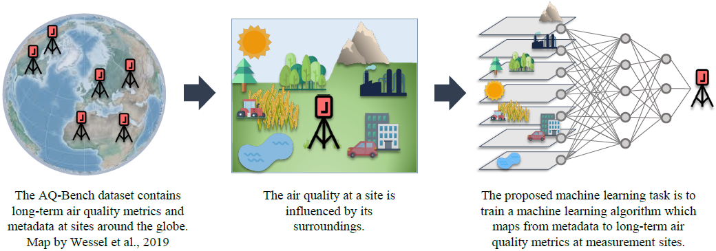
With the AQ-Bench dataset, we contribute to the recent developments towards shared data usage and machine learning methods in the field of environmental science. The dataset presented here enables researchers to relate global air quality metrics to easy-access metadata and to explore different machine learning methods for obtaining estimates of air quality based on this metadata. AQ-Bench contains a unique collection of aggregated air quality data from the years 2010–2014 and metadata at more than 5500 air quality monitoring stations all over the world, provided by the first Tropospheric Ozone Assessment Report (TOAR). It focuses in particular on metrics of tropospheric ozone, which has a detrimental effect on climate, human morbidity and mortality, as well as crop yields. The purpose of this dataset is to produce estimates of various long-term ozone metrics based on time-independent local site conditions. We combine this task with a suitable evaluation metric. Baseline scores obtained from a linear regression method, a fully connected neural network and random forest are provided for reference and validation. AQ-Bench offers a low-threshold entrance for all machine learners with an interest in environmental science and for atmospheric scientists who are interested in applying machine learning techniques. It enables them to start with a real-world problem relevant to humans and nature. The dataset and introductory machine learning code are available at https://doi.org/10.23728/b2share.30d42b5a87344e82855a486bf2123e9f (Betancourt et al., 2020) and https://gitlab.version.fz-juelich.de/esde/machine-learning/aq-bench (Betancourt et al., 2021). AQ-Bench thus provides a blueprint for environmental benchmark datasets as well as an example for data re-use according to the FAIR principles.
- Article
(1812 KB) - Full-text XML
- BibTeX
- EndNote


In recent years, machine learning has achieved remarkable success in areas such as pattern, image and speech recognition by usage of increasing computing power, innovative algorithms and high data availability (Krizhevsky et al., 2012; Amodei et al., 2016; Silver et al., 2016). This has aroused the interest of environmental scientists in exploring the application of machine learning and data-driven methods in their fields. The strength to be exploited is the ability of machine learning algorithms to find complex relationships in large multivariate, inhomogeneous datasets (as described, for example, in Wise and Comrie, 2005; Porter et al., 2015).
In air quality research, there is one pollutant which is especially challenging to track: tropospheric ozone, a toxic trace gas which harms human health and vegetation and also impacts the climate (Cooper et al., 2014; Monks et al., 2015). Tropospheric ozone is difficult to track because it has no direct emission sources but is produced as a secondary airborne pollutant by several chemical reaction chains involving a large variety of precursors and photochemistry. With a lifetime of days to weeks (Wallace and Hobbs, 2006), the ozone concentration is affected by various physical and chemical processes which produce and destroy ozone. Therefore, ozone is a scientifically interesting candidate for machine learning applications: it is influenced by many interconnected environmental factors – and it is interesting to see if machine learning algorithms can learn these.
Data-driven atmospheric chemistry research was combined with machine learning from the late 1990s to model and predict surface ozone concentrations in an alternative way to multivariate regression (Yi and Prybutok, 1996; Comrie, 1997; Elkamel et al., 2001; Caselli et al., 2009). These data-driven approaches take ground-based measurements as input and predict the pollutant concentrations for the following days at individual locations. The principle behind recent machine learning applications in ozone research is often a similar principle to the one Schultz et al. (2021) described for weather data: the input data are directly mapped to a specific data product, e.g., from meteorological and past ozone measurements to the next day's maximum ozone value. In recent studies, Sayeed et al. (2020) and Kleinert et al. (2021) predicted regional ozone time series with convolutional neural networks and meteorological input data. Furthermore, Silva et al. (2019) trained a feed-forward neural network to output ozone dry deposition at two forest measurement sites. Moreover, within computationally complex components of atmospheric chemistry models, machine learning techniques are used as emulators or surrogate models. They replace for example costly atmospheric chemistry and micro-physical calculations to improve computational performance of the models (Kelp et al., 2020). In addition, machine learning is applied in the calibration of low-cost sensors for air quality measurements in order to account for the diverse sources of interference with these measurements (Schmitz et al., 2021; Wang et al., 2020). Nevertheless, to our knowledge there are currently no machine learning projects that attempt to analyze and predict ozone on the global scale, for longer time periods and with many kinds of metadata.
Developments in machine learning are accelerated by the existence of precompiled benchmark datasets that allow machine learners to try out specific tasks, exchange solutions and compete with each other (LeCun et al., 2010; Deng et al., 2009; Rasp et al., 2020). Benchmarks can also be used for the development of explainable artificial intelligence approaches (Kierdorf et al., 2020; Roscher et al., 2020). So far, few such benchmark datasets exist in the field of environmental science, especially related to air quality. While air quality data are in principle easily accessible from a variety of archives, there is often incomplete information and insufficient metadata to develop useful machine learning applications from these data. Furthermore, harmonization of such data from different sources, which is needed to achieve a global picture of ozone air pollution, is a difficult and time-consuming task.
With the AQ-Bench dataset, we aim to fill this gap and provide a dataset of global long-term air quality metrics and metadata compiled from the TOAR database (Tropospheric Ozone Assessment Report; Schultz et al., 2017). To make these data usable for machine learning developments, this paper also describes the specific task of mapping between the metadata and the air quality metrics (see graphical abstract). Our ready-to-use, fully documented dataset is freely available under the DOI https://doi.org/10.23728/b2share.30d42b5a87344e82855a486bf2123e9f (Betancourt et al., 2020). We also provide our baseline machine learning code at https://gitlab.version.fz-juelich.de/esde/machine-learning/aq-bench (Betancourt et al., 2021), offering a low-threshold entrance to machine learning in environmental science within a relevant research topic. In Sect. 2 of this paper we present the main factors affecting tropospheric ozone as the scientific background for the design of the AQ-Bench dataset. Section 3 introduces the TOAR data products from which AQ-Bench was constructed. In Sect. 4, we describe the dataset itself. Section 5 contains the machine learning task for AQ-Bench and three baseline experiments to evaluate the applicability of these data in the machine learning context. We discuss opportunities and challenges of AQ-Bench and give problem-related expected difficulties in Sect. 6. Information on data and code availability is given in Sect. 7, followed by a conclusion in Sect. 8.
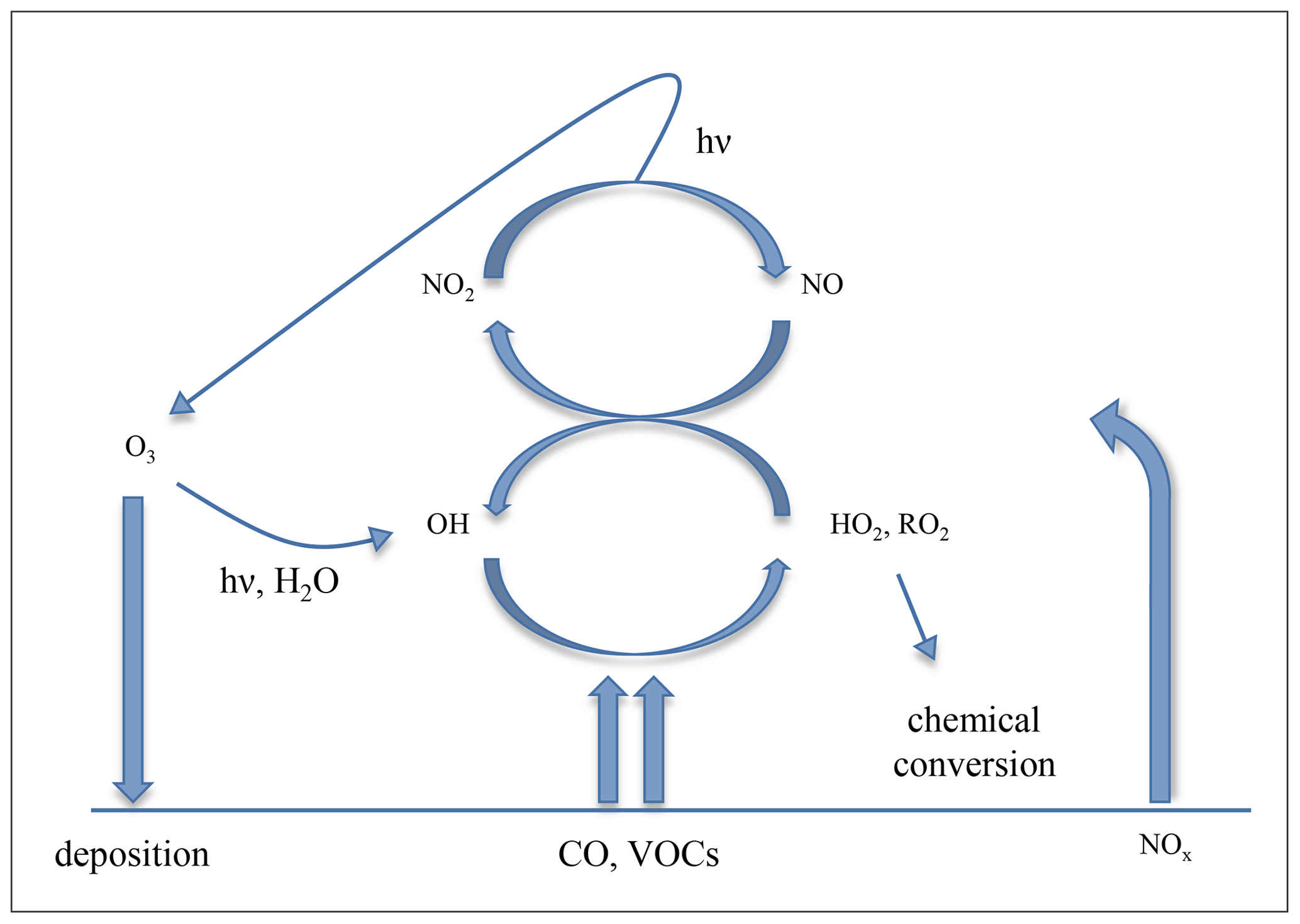
Ozone (O3) is a toxic greenhouse gas. While stratospheric ozone protects life on the planet's surface from ultraviolet radiation, tropospheric ozone is detrimental to human health, vegetation and climate. The AQ-Bench dataset and this paper focus exclusively on tropospheric ozone, more precisely the near-surface ozone to which humans, animals and plants are exposed. Ozone is a secondary pollutant that is formed from emissions of precursor substances and undergoes a variety of physical and chemical processes during its atmospheric lifetime. Figure 1 summarizes these processes, and they are further elaborated in the following subsections. How the described processes translate into the data in AQ-Bench is described in the dataset description (Sect. 4).
2.1 Precursor emissions
The most important ozone precursors are nitrogen oxides, carbon monoxide and volatile organic compounds (denoted as NOx, CO and VOCs in Fig. 1; note that NOx = NO2 + NO). Many of these precursors are emitted by human activities, e.g., from traffic, industry and agriculture (Benkovitz et al., 1996; Field et al., 1992). NOx concentrations resulting primarily from combustion processes are especially high at very heavily polluted sites such as in city centers or near power plants. Industrial and traffic pollution are closely related to energy consumption depending on population density and economic activities. Agriculture machinery emits similar trace gases to those emitted by traffic or industry. Moreover, agricultural plants are often fertilized, which adds more trace gas emissions (Veldkamp and Keller, 1997). In addition to emissions from human activities, several processes in nature also lead to emissions, especially of VOC compounds. For example, plants emit VOCs which are often more reactive (and could therefore produce more ozone) than VOCs emitted from human activities. The exact emission patterns vary among the types of plants and are thus related to land cover. Agricultural fields, forests and grasslands therefore yield different magnitudes and seasonal cycles of VOC emissions (Simpson et al., 1999). Emissions can also occur from oceans, barren land, and snow- or ice-covered surfaces. For example, the latter emit substantial quantities of NOx in Arctic regions (Wang et al., 2007).
2.2 Ozone chemistry
The daily average ozone volume mixing ratios vary in the order of 10 to 100 ppbv (parts per billion by volume), with a lifetime of days to weeks (Wallace and Hobbs, 2006). Ozone has practically no direct emissions but is exclusively formed through atmospheric chemical reactions. The chemical processes leading to ozone formation are driven by ultraviolet radiation (denoted with hν in Fig. 1). At wavelengths <0.43 nm, photons convey enough energy to release chemical bonds in nitrogen dioxide (NO2) molecules. This process (photo dissociation) leads to the formation of nitrogen oxide (NO) and a free oxygen radical (O). NO is also a radical and thus recombines quickly, while O collides with a high probability with O2 and forms O3. The produced O3 is removed rapidly when it reacts with NO to NO2 + O2. The reactions form a null cycle, because O3 is both created and destroyed. The cycle stabilizes at a certain O3 concentration, depending on the available NO2, ultraviolet light intensity and temperature. Up to a certain point, the ozone concentration rises with increasing NO2 concentrations.
The dynamic equilibrium of this cycle can be altered by the presence of VOCs and CO (denoted as primary emissions in Fig. 1), which provide chemical pathways to convert NO to NO2 without the destruction of O3 by oxidation (oxidized pollutants denoted as HO2 and RO2 in Fig. 1). This leads to a nonlinear system, where O3 concentrations depend on the ratio of VOCs + CO and NOx (= NO + NO2) concentrations. During the daytime, O3 can photo dissociate and recombine with water vapor (H2O in Fig. 1), thereby forming hydroxy radicals (OH in Fig. 2) which fuel a large share of atmospheric oxidation. There are several thousand chemical reactions occurring in the atmosphere, which need to be considered for an adequate description of ozone formation and loss processes, and Fig. 1 only provides a very small glimpse into this rather complex system. For more details on ozone chemistry we refer to Brasseur et al. (1999).
2.3 Transport and loss processes
During its atmospheric lifetime, O3 can be transported on spatial scales of hundreds or even thousands of kilometers (Schultz et al., 1999), until it is removed via atmospheric chemical reactions and deposition (indicated with downward-pointing arrows in Fig. 1). Primary chemical loss of O3 is rather indirect via removal of NO2 in polluted regimes and radical–radical reactions in clean environments with low NO2 concentrations. Besides the chemical loss, O3 can be removed by deposition on surfaces, especially on the leaves of natural or agricultural plants (Emberson et al., 2000). Ozone irreversibly damages plant tissue when the plant leaves take it up (Schraudner et al., 1997), leading to reduced crop yields (Mills et al., 2011). Ozone deposition on water surfaces is relatively slow, but due to the large extent of them, this process also matters in the context of the global ozone budget (Luhar et al., 2018).
2.4 Interconnected factors
In the following, we describe how the influences of ozone precursor emission, chemistry, transport and loss (described in Sect. 2.1–2.3) can come together. The combination of chemistry and transport of air pollutants favors ozone formation downwind of sites with high precursor exhaust. A typical example is summertime rural areas downwind of larger city centers, where peak ozone values can often be observed (Xu et al., 2011). In the close vicinity of power plants or in city centers, NOx is often very high and low ozone levels are observed (Sillman, 1999).
There are several geographical factors which determine the rates of chemical formation and loss of ozone. These factors can result in different mixes of ozone precursor emissions, varying reaction rates and varying rates of deposition. For example, the climate in a certain location determines the vegetation cover and the local weather. Since temperatures near the Equator are high and more intense sunlight is available, ozone levels are generally higher there than near the poles. Moreover, at higher altitudes the air is generally cooler and drier, which leads to changes in reaction rates. Local flow patterns can also influence the ozone concentration, for example through the transport of air masses from valleys to mountain tops (Kaiser et al., 2007).
Besides natural geographic factors, political decisions can also influence ozone formation. Many governments and decision makers worldwide strive to reduce air pollution by emission regulation, but these regulations differ between countries and may be implemented with more or less rigor. Ozone regulation is more difficult than that of primary air pollutants as one has to limit both VOC and NOx emissions in order to control ozone, because of the chemical cycles described in Sect. 2.2.
Although ozone has a rather long lifetime, the local ozone concentration can change substantially in a matter of minutes and on scales of meters (e.g., in a street canyon), but it can also remain stable across hundreds of kilometers and for several weeks (e.g., at higher altitudes over the oceans). The “radius of influence” within which ozone is determined by nearby precursor emissions and deposition surfaces is typically about 25 km in mid-latitude areas (European Union, 2008). All in all, ozone concentrations measured at a station are determined by many interconnected influences from precursor emissions, land use and land cover, and the local weather conditions. Many of these factors are poorly quantified, and often the interconnections have not yet been understood well (Schultz et al., 2017). With AQ-Bench and the machine learning task described below, we want to explore a novel way of using a multitude of geographical features to predict ground-level ozone around the world. The details of data selection are described in Sect. 4, while the machine learning task is provided in Sect. 5.1.
The TOAR database (Schultz et al., 2017) was created in the context of the Tropospheric Ozone Assessment Report (TOAR). It contains one of the world’s largest collections of near-surface ozone measurements, gathered from public bodies, research institutions and air quality networks all over the world. TOAR data products enabled the first comprehensive global assessment of the tropospheric ozone distribution and trends (Schultz et al., 2017; Fleming et al., 2018; Gaudel et al., 2018; Lefohn et al., 2018; Chang et al., 2017; Young et al., 2018; Mills et al., 2018; Tarasick et al., 2019; Xu et al., 2020). In the spirit of FAIR data usage (Wilkinson et al., 2016), these data products are openly available via the JOIN graphical interface1, a REST interface2 and the PANGAEA repository3.
For the AQ-Bench dataset, we selected and harmonized air quality metrics and metadata from TOAR (see Sect. 4 and Appendix C). This section therefore contains a description of these selected data products, introducing the concepts of metrics and metadata.
3.1 Air quality metrics
The TOAR database contains hourly ozone measurements, transmitted from air quality observation sites. The data providers conduct quality control on these data by calibrating the measurement devices and setting suitable instrument parameters. In a second step of data curation, the TOAR database administrators conduct a statistical analysis of the data to identify and remove low-quality data (Schultz et al., 2017). Hourly data are usually aggregated into statistics or “metrics” for further analysis. Ozone metrics consolidate air quality properties of longer time series (e.g., a season or a year) into a single figure, which can then be directly used for a scientific assessment and in decision-making. Longer aggregation periods also average out short-term weather fluctuations. There are specific metrics for different areas of ozone impact assessments (respiratory and cardiovascular disease, vegetation damage, climate impacts) and control.
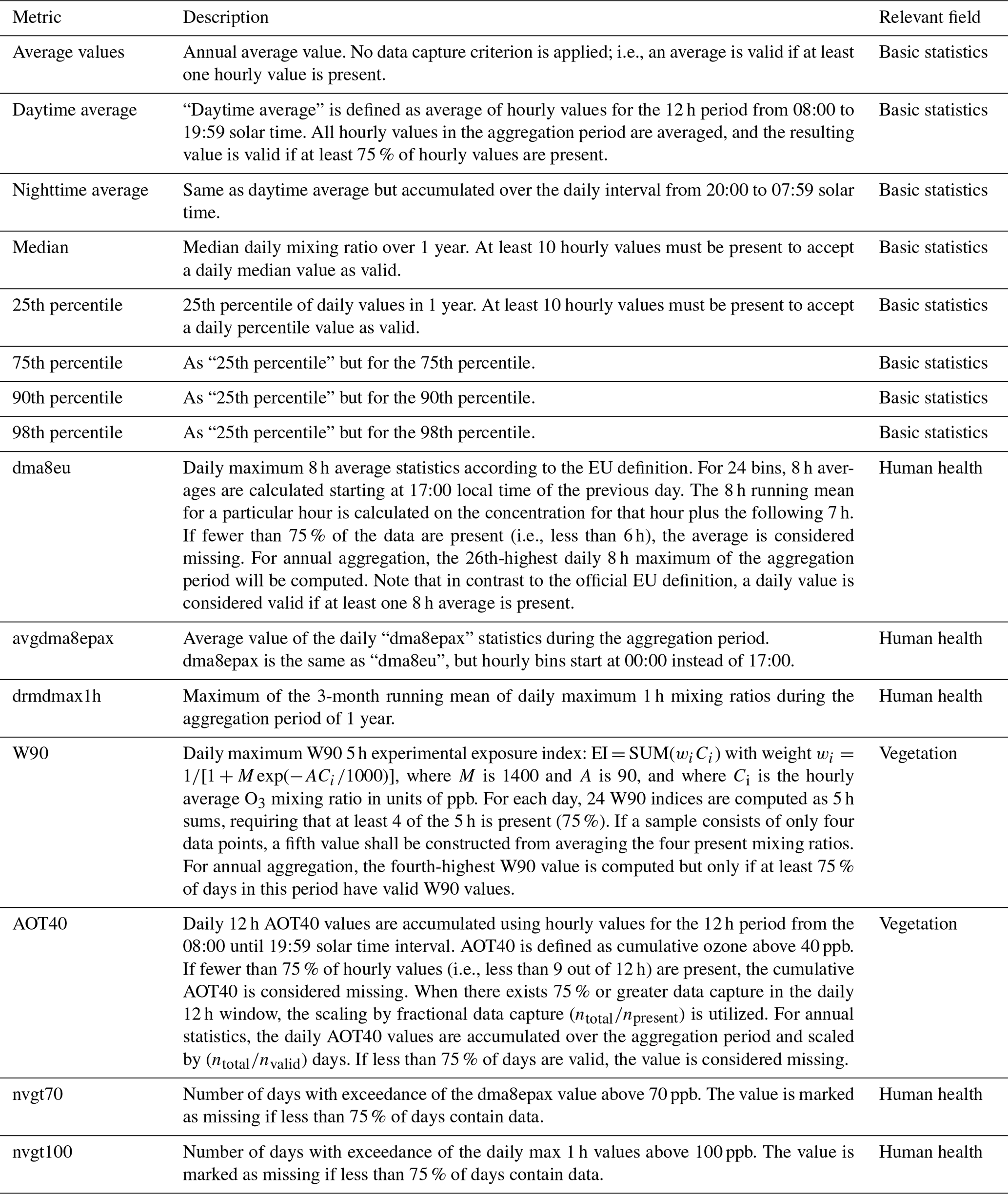
The JOIN web service is connected to the TOAR database and provides more than 30 of the most frequently used metrics as data products, calculated on-demand from hourly data. Besides these specialized metrics, basic statistics such as averages, medians and percentiles are also available in JOIN. In the context of evaluating air quality, the validity of reported ozone metrics hinges on the data capture. Typically, statistical aggregations (i.e., metrics) of air quality data can only be used for decisions on attainment or non-attainment of air quality standards if at least 75 % of the (hourly) samples in a dataset were reported. In this sense, the validity of ozone metrics is tied to the data completeness, and we will use the term “valid data” to indicate samples with sufficient coverage of accurate data. All metrics which are part of AQ-Bench are listed in Table 2 of Sect. 4. Documentation and further information on all available metrics including data capture criteria are available in Schultz et al. (2017) and Lefohn et al. (2018).
3.2 Station metadata
The TOAR database also contains geographical information on air quality measurement station locations, i.e., station metadata. Metadata give background information on the measurement site where the data were retrieved from and thus enable the characterization of the location. These metadata are collected from different sources. Some data, for instance station coordinates and altitude, are given by the data providers and quality controlled by TOAR. Others were derived from data sources with individual quality control, such as satellite Earth observations. For a complete list of the available metadata attributes see Schultz et al. (2017) and the REST interface (see footnote 2).
For the AQ-Bench dataset described in this paper, we selected metadata from the TOAR database which characterize measurement locations and their surroundings with respect to pollution-relevant properties as introduced in Sect. 2. They are listed in Table 1 of Sect. 4.
The AQ-Bench dataset consists of metadata and aggregated ozone metrics from the years 2010–2014 at 5577 measurement stations all over the world, compiled from the TOAR database. The point of interest is to determine the resulting ozone metrics (see Sect. 3.1) given all environmental influences (Sect. 2) represented by metadata (Sect. 3.2). Our contribution in data preparation is to pick metadata with expert knowledge, relate them to processes, and aggregate air quality data to metrics in a way that it is representative of long time periods and meaningful in a machine learning context.
Three key points in the conception of this benchmark dataset are as follows: (1) as targets, we use aggregated air quality metrics over 5 years. These are not influenced by short-term weather and emission forcings but by site conditions on the climatological timescale. (2) Many known environmental influences on ozone are on short timescales (see Sect. 2), but we aim to predict long-term air quality conditions at the sites. Thus, we have identified which station metadata are the climatological representations of these short forcings. (3) We use a – to our knowledge unprecedented – variety of metadata that contain diverse information about environmental influences on the climatological scale. These metadata are sometimes not directly descriptive of the influences but rather proxies for them. The benefits of machine learning must be leveraged to relate these proxies to air quality metrics.
This aggregated, climatological approach makes it possible to cover air quality data over a long period of time on the global scale with a relatively small and compact dataset. Yet, aggregated data account for long-term air quality conditions at a site, and daily or hourly influence on ozone variations is not considered. Figure 2 gives an overview of all TOAR air quality monitoring stations included in AQ-Bench.
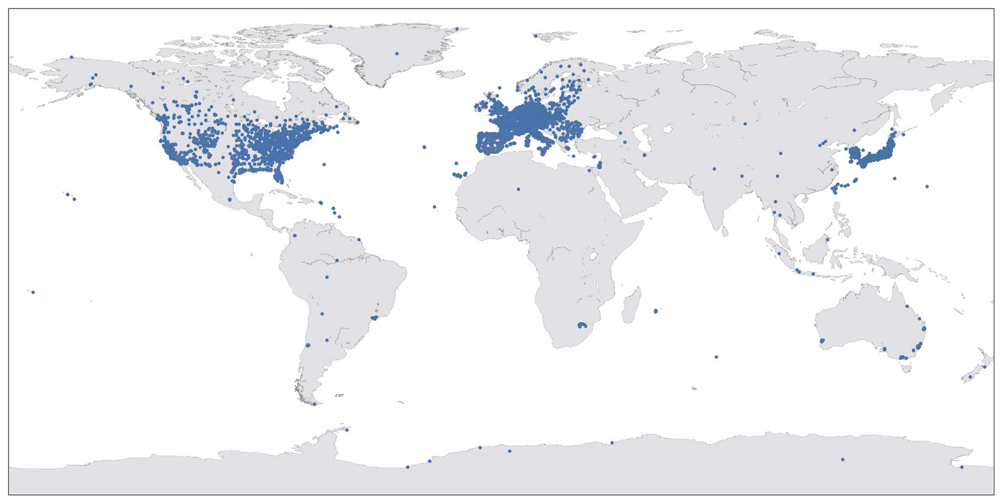
Figure 2Worldwide measurement stations which are part of AQ-Bench, selected from the TOAR database. Map by Wessel et al. (2019).
4.1 Station metadata
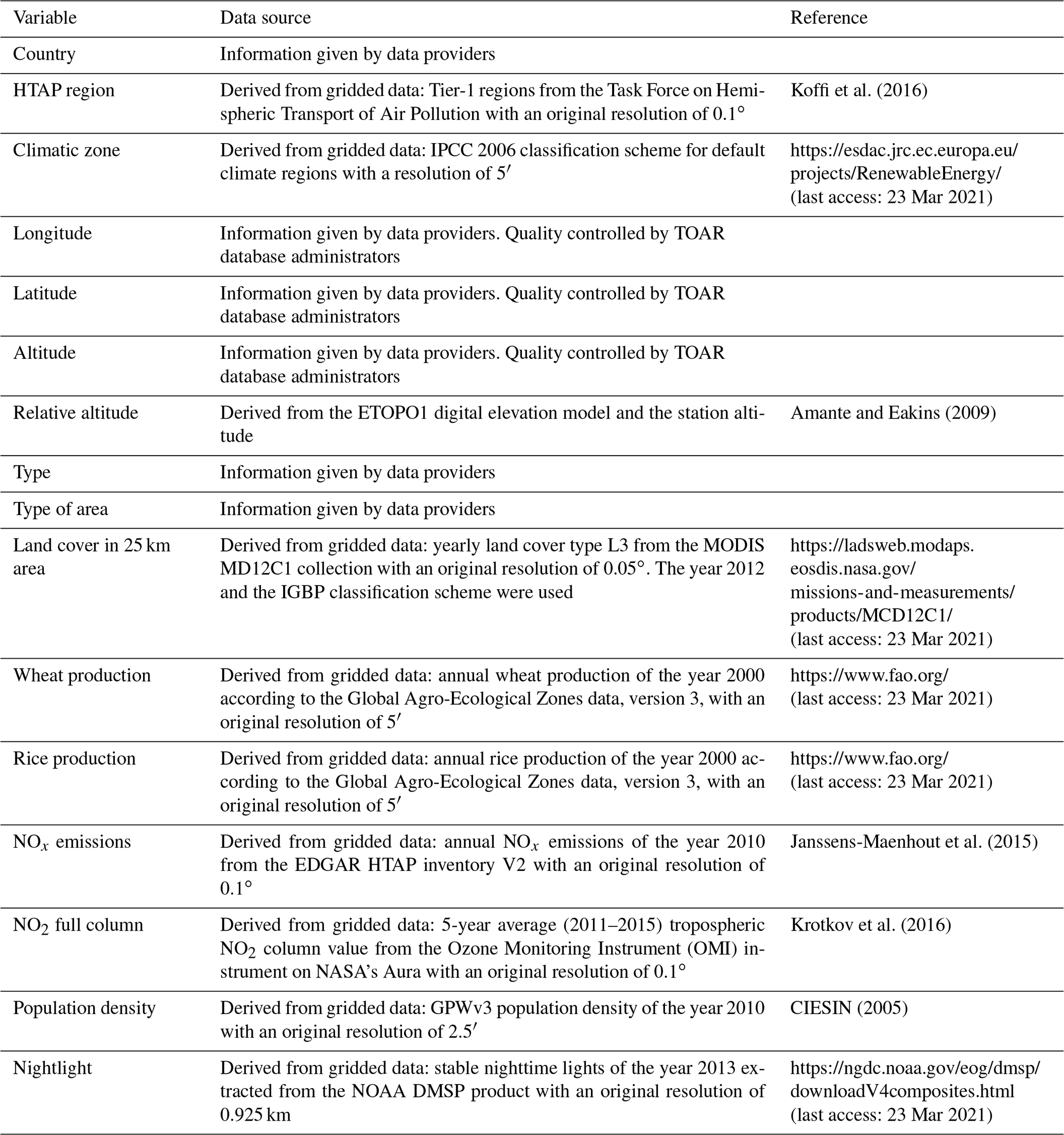
A summary of metadata in AQ-Bench is given in Table 1. The data originate from the TOAR database (Sect. 3); see Appendices A and C for details on the data sources and harmonization for machine learning purposes. The metadata contain proxies for environmental influences on ozone on the climatological scale. In the following, we give two examples.
As mentioned in Sect. 2, ozone is influenced by weather. Likewise, ozone on longer timescales is influenced by climate. One variable in the AQ-Bench dataset is the climatic zone in which the site is located. The climatic zone provides simplified information about climatic conditions at a location, for example, whether it is hot or cold, humid or dry, or of tropical climate.
A second example is ozone precursor emissions. In Sect. 2.1 we outlined that they are emitted by, for example, traffic and human activities. This means that the population density at a site is a good proxy for these activities. A second – more subtle – proxy is the stable nightlight at a location. This is the average intensity of light during the night as seen from space, an indicator for industrial activity. In Sect. 2.2, we pointed out that ozone is often formed downwind of sites with high human and industrial activity. Therefore, in the AQ-Bench dataset, we give not only population density and stable nightlights at a site but also related statistics of the closer surroundings. One example is the maximum population density in a radius of 5 km around the station.
All variables of the AQ-Bench dataset can be related to environmental impacts on the climatological timescale. We indicate the proxies in the right column of Table 1. Machine learning can make use of these proxies, even if they are not directly related to ozone concentrations.

4.2 Ozone metrics
The AQ-Bench dataset contains annually aggregated, averaged (years 2010–2014) ozone metrics as introduced in Sect. 3.1. There are therefore two steps involved in obtaining the metrics: (1) obtaining up to five yearly metrics between 2010–2014 from hourly measurements, including data cover criteria to validate the metrics, and (2) averaging over these 5 years. If fewer than two yearly values are available, the value is considered missing. Missing values are denoted with −999 in the dataset. Some suspiciously high values were eliminated, as documented in Appendix C. A summary of all metrics and their data capture criteria is given in Table 2. More details on the process of ensuring robustness through data capture are given in Appendix B.
Table 2The ozone metrics of AQ-Bench. The unit is ppb (parts per billion) for all metrics except the nvgt metrics, where it is the number of days.
In this section, we introduce the AQ-Bench dataset as a machine learning benchmark dataset. This means we combine the data documentation from the previous section (Sect. 4) with the machine learning task for this dataset. We also provide an evaluation metric, a data split and baseline experiments.
5.1 Task description and evaluation metric
The task proposed for the AQ-Bench dataset is to train a machine learning model that maps from metadata in Table 1 to the ozone metric values in Table 2. This can be achieved with individual machine learning algorithms or in one multi-output algorithm.
The evaluation metric for our baselines is R2, the coefficient of determination:
where m denotes a sample index, M denotes the total number of samples, denotes a predicted output value and ym denotes a reference target value.
R2 measures the proportion of variance in the output values that the model predicts from the input values. A larger R2 thus denotes a better model, and the largest possible value is 1, or 100 %. We choose R2 as it is comparable between all different targets, even if they cover different value ranges. The overall score of the solution is the mean of all scores achieved on the test set for all ozone metrics. For further evaluation of machine learning results, cross validation can be applied. We would like to challenge the machine learning and air pollution researchers to use this rather small dataset as efficiently as possible to extract all inherent information to accurately map onto the ozone metrics.
5.2 Data split
We provide a fixed data split within the AQ-Bench dataset to enable a comparison of our baseline results with future solutions and to provide a suitable data setup for learning (see below). As it is good practice in machine learning, the dataset is split into three subsets for training, validation and hyperparameter tuning, and testing. The three data subsets are required to be independent while having a similar statistical distribution to prevent the concealment of possible overfitting and an overestimation of accuracy. Because the dataset is relatively small, the split was chosen to be 60 %–20 %–20 %, as is commonly used for datasets of this size. It is indicated in the dataset whether an example belongs to the training, validation or test set.
In order to guarantee the spatial independence of the subsets, the data are divided into several spatial zones. The zones were created by spatial clustering, where stations are assigned to the same cluster if they are closer than 50 km to each other (European Union, 2008). Large station clusters were split again into smaller ones to ensure similar statistical distributions of the training, validation and test datasets. The final clusters were randomly assigned to the three datasets. This way, all stations within a spatially dependent cluster are allocated to the same dataset.
5.3 Baseline experiments
As baselines for machine learning approaches on the AQ-Bench dataset, we present results obtained with three standard machine learning algorithms. For preprocessing, rows with missing values are dropped. Continuous metadata are scaled, each by a quantile range from 25 % to 75 % to avoid influence from outliers. Categorical metadata are one-hot encoded, resulting in 135 input features in total. We drop the longitude from our baseline experiments, since this is a circular variable and cannot be used without additional feature engineering. The preprocessed metadata are called input data in the following. Ozone metrics, which are the targets, are not scaled.
Methods are as follows:
-
Linear regression. Linear regression models the simplest correlation between input and target values. It maps an input data example xm with , where w and b are the regression parameters weights and bias. Vector has the dimension of input vector .
-
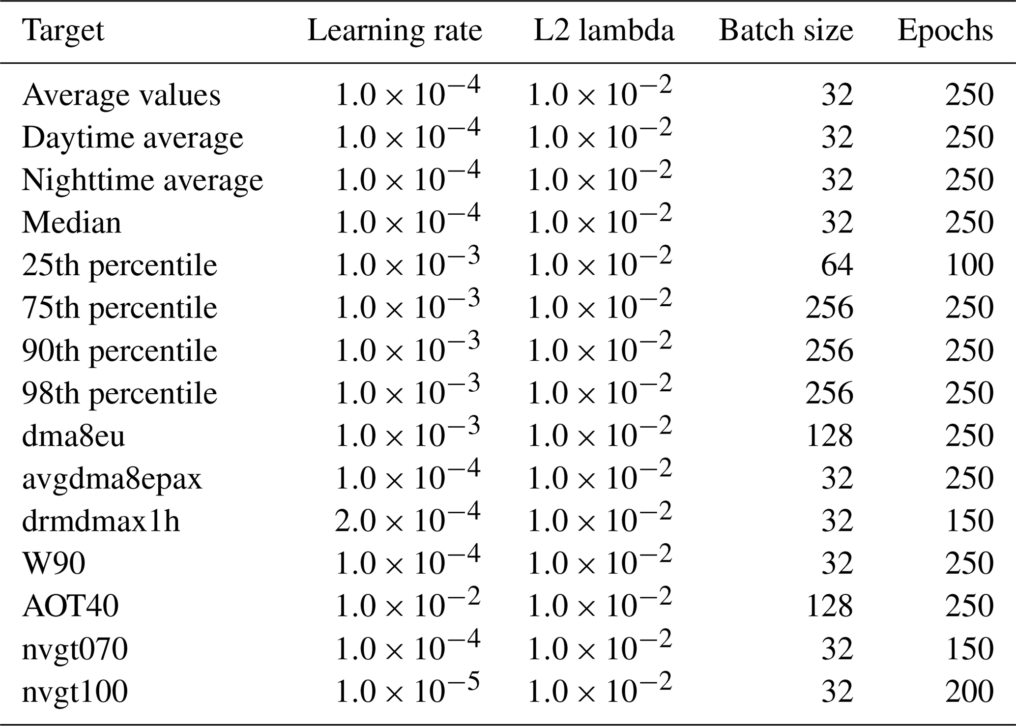
Neural network. We train a shallow fully connected neural network with two hidden layers of size 20 and 5 neurons, respectively. We use the Adam optimizer with an MSE (mean squared error) loss function, L2 regularization and ReLU (rectified linear unit) as the activation function (Goodfellow et al., 2016). Training is performed independently for each ozone metric. We optimized the learning rate and regularization parameter by empirical studies and random search. Through further empirical analyses, we decided on the hyperparameters summarized in Appendix B. The model is written in TensorFlow–Keras (Chollet et al., 2015).
-
Random forest. Our random forest model (Breiman, 2001) is built with a number of 100 trees for each target, based on empirical studies. As in the case of the neural network, we use the MSE as an optimization criterion. We use the RandomForestRegressor of scikit-learn (Pedregosa et al., 2011).
The baseline results are summarized in Table 3. Comparing the different models, random forest yields the best results for all targets except the nvgt metrics, where the neural network performs best. The linear regression is the worst for most targets except, e.g., 75th percentile, where it is the second best after the random forest. For some targets, e.g., average values, random forest is only slightly better than the neural network. However, there are targets, e.g., AOT40, where the gap between the two methods is almost 10 %. The neural network performs best for nvgt070 and nvgt100. The baseline experiment results of nvgt100 drops in comparison to other targets with partly negative R2 scores. The results of nvgt070 have the second-lowest scores. These two targets count exceedances of a certain threshold, so many values equal zero, which might be problematic for standard machine learning algorithms to capture. Except for those, R2 is higher than 50 % for at least one of the three models per target. This shows that there is a quantitative relationship between input data and targets. Nevertheless, for our baseline experiments we used rather simple models in order to prove the concept. Ozone, as a secondary pollutant with levels highly dependent on the environment and available precursors, is not captured perfectly by these simple baselines.
Table 3R2 scores of the test set in percent. Best results are marked in bold; second-best results are underlined.

6.1 Opportunities for machine learning in air quality research
With the AQ-Bench dataset, we used our knowledge on environmental influences on ozone, a toxic greenhouse gas, to bundle air quality data and metadata with machine learning approaches. By doing this, we enable a quick entry into machine learning in air quality research on a global scale with reduced machine learning overhead. Our approach enables the use of data from various sources that would otherwise be time-consuming to acquire and prepare. We provide a ready-to-use dataset for the machine learning community to support research on meaningful real-world applications (motivated by Wagstaff, 2012).
One great advantage of using machine learning for air quality research is the possibility of using data from various different sources, especially data which are not directly connected to air pollution via physical or biogeochemical models (e.g., stable nightlights). To explore this opportunity for ozone, we gathered an unprecedented variety of metadata to allow the machine learning approaches to obtain hints on the many interconnected, nonlinear influences, which determine ozone concentrations (see Sect. 2). As the results from our baseline experiments show, the AQ-Bench dataset bears some potential to exploit these relations with machine learning methods.
Currently not many air pollution researchers use purely data-driven approaches for their studies. With AQ-Bench we offer a first data-driven machine learning view on global tropospheric ozone. To achieve the global view, we use the JOIN web interface4 of the TOAR data center, which provides customized data products from the TOAR database. As proposed by Schultz et al. (2021), our approach is to output the demanded metrics directly and thus to obtain the required data products directly from machine learning. Further applications of AQ-Bench could be developed, such as a classification of ozone sites into “healthy” or “unhealthy”. Our dataset fits with the vision for benchmark datasets described by Ebert-Uphoff et al. (2017).
6.2 Limitations of AQ-Bench
AQ-Bench includes ozone metrics and metadata from 5577 stations and spans a time period of 5 years. The stations included in AQ-Bench are not distributed equally around the globe. The spatial coverage in most of the regions is low, except in the USA, European countries and some regions of East Asia (Japan and South Korea). This raises the question of whether it is possible to generalize machine learning results to regions that are not included in the training data, even if they have similar input metadata. Possibly it may be necessary to use a combination of observational data and numerical models to achieve full global coverage (cf. Chang et al., 2017).
Measurement errors, interannual changes and drift result in noisy ozone metrics. Conversely, at least in the current version of AQ-Bench, the input metadata are fixed and have no temporal evolution, an assumption which we can make because we average over 5 years of ozone metrics. It cannot be ruled out that within this time major environmental changes could have happened; e.g., settlements could grow or shrink during this time. This means, that metadata as given in AQ-Bench might not be valid for the whole time period of 5 years. The population density might have increased; the climate zone might have changed; and if a forest was cleared, for example, the land cover would have changed as well. We note that some uncertainty is introduced by the relatively lax requirement of two annual ozone metric values to form a valid 5-year average value (see Appendix B): if both yearly averages correspond to the beginning or to the end of the time period in question, a bias may be introduced if the ozone concentrations exhibit a strong trend or if the region experienced rapid changes, such as urbanization.
Another topic is the complexity of the problem, compared to the dataset size. It is doubtful whether simple machine learning models are intricate enough to grasp all complex relationships between ozone and environmental factors. On the other hand, very deep neural networks, which may be capable of learning such patterns, cannot be trained on a dataset with only 5577 samples. In Sect. 5.3 we gave some basic machine learning approaches to find a mapping between the metadata and the target ozone metrics. We assume that the inaccuracies in our baselines partly arise from the complex relationships of ozone with the environment compared to the input dataset size and complexity of these basic machine learning approaches. Furthermore, through a longer aggregation period, we emphasize robust, static features. This aggregation reduces the size of the dataset and makes global coverage possible. Due to our focus on spatial relationships we consciously ignore time-resolved patterns. We simplify the problem and make machine learning on the dataset easy – but this simplification also comes at the cost of introducing noise and uncertainties. For a more complete description of ozone processes, more input data, additional input variables and time-resolved data could be used.
6.3 Machine learning challenges arising from AQ-Bench
In order to provide some guidance on how the machine learning results could be improved compared to the standard machine learning methods applied in our baselines (Sect. 5.3), we briefly discuss some techniques here. One aspect to explore is feature engineering. Currently AQ-Bench includes for example the circular variable longitude, which cannot be accessed by the machine learning algorithm without further feature engineering. Other variables could be accumulated, or transformed to improve machine learning results. See, e.g., Duboue (2020) for an introduction to the topic. We hope that the research community will be creative in feature engineering.
Another aspect is multi-task learning. The baseline methods were performed independently for each ozone metric, but there may be a connection between them, as they all describe ozone pollution. Therefore, multi-task learning is a promising direction to exploit these connections. See Zhang and Yang (2017) for a review on this topic.
The baseline experiments show that extremes are sparse and thus difficult to catch. For example, the metric nvgt070 which counts the days where maximum ozone exceeds 70 ppb (which happens at least once a year at approx. 75 % of the stations) gives acceptable results, but nvgt100 is not captured well. This is explained by the fact that there are very few (<25 %) stations which experience occasional ozone values above 100 ppb. Extremes can be captured by imbalanced learning. See He and Garcia (2009) for a review on learning from imbalanced data.
The AQ-Bench dataset is available in .csv format at http://doi.org/10.23728/b2share.30d42b5a87344e82855a486bf2123e9f (Betancourt et al., 2020). To enable a machine learning quick start on the AQ-Bench dataset with reproduction of the baseline experiments, we also provide an introductory Jupyter notebook on https://gitlab.version.fz-juelich.de/esde/machine-learning/aq-bench (Betancourt et al., 2021). To start it directly in your browser, click the button “launch on binder” in the readme of this repository.
In this paper, we introduced AQ-Bench as a benchmark dataset for machine learning on global air quality metrics. It allows the exploration of different machine learning methods on the real-world problem of air quality analyses. Specifically, the machine learning task is to map station metadata to air quality metrics at 5577 measurement stations around the globe and to optimize the results with hyperparameter tuning and data engineering. The usability of the dataset is documented through the results from our three baseline machine learning solutions. These methods show robust relations between the input data (geospatial features) and the targets (ozone metrics), and these relations are understandable from an atmospheric chemistry point of view. As data-driven techniques for air quality research are emerging, we present a first benchmark dataset on the global scale. The purpose and significance of AQ-Bench is twofold: first, it has never been tried before to exploit a rich collection of geospatial datasets to find out which fraction of ozone pollution can be attributed to such more or less static geographical features. Second, this problem definition makes some low-level air quality analysis easily accessible to data scientists with little or no background in atmospheric chemistry. Following the vision of Ebert-Uphoff et al. (2017) to design benchmarks that bridge geoscience and data science, the key features of AQ-Bench are as follows:
-
Active research area. Ozone is a highly relevant and active field of research, as it harms living beings and the ecosystem. Ozone research benefits from making data available and developing data-driven methods for ozone assessment.
-
Understandable context. We introduced the complex mechanisms behind ozone formation as well as physical and chemical processes in Sect. 2 to make the scientific context of this dataset understandable to everyone, even without prior knowledge.
-
Impact on data science. Since AQ-Bench is relatively small and thus easy to handle, it is suitable for beginners in programming. AQ-Bench can be trained in less than a minute on a common personal computer without GPUs, so one can quickly iterate through different algorithms and configurations. Yet noise, the small size of the dataset and the complicated underlying processes make it challenging to achieve satisfactory machine learning results on this dataset.
-
A means to evaluate success. We propose R2, the coefficient of determination, as an evaluation metric for AQ-Bench. It is a suitable metric because it measures the proportion of variance in the output values that the model predicts from the input values. It is comparable between all targets.
-
Quick start. To start machine learning on AQ-Bench in a common browser, launch the “binder” in the following Git repository: https://gitlab.version.fz-juelich.de/esde/machine-learning/aq-bench (last access: 21 June 2021). Running the introductory notebook on the binder enables users to try out different training algorithms and hyperparameters directly in the browser.
-
Citability and reproducibility. The dataset has a DOI, and the baseline experiments can be reproduced with the code that is openly available on GitHub (see Sect. 7).
We hope that the AQ-Bench dataset will help to advance data-driven techniques in the field of air quality research and form a basis for future experiments and research.
Table A1Technical details on the station metadata of the AQ-Bench dataset, updated from Schultz et al. (2017). Please note that in order to keep this table uncluttered, we have summarized all types of land cover in a 25 km area, all population density and all nightlight variables in one row each.
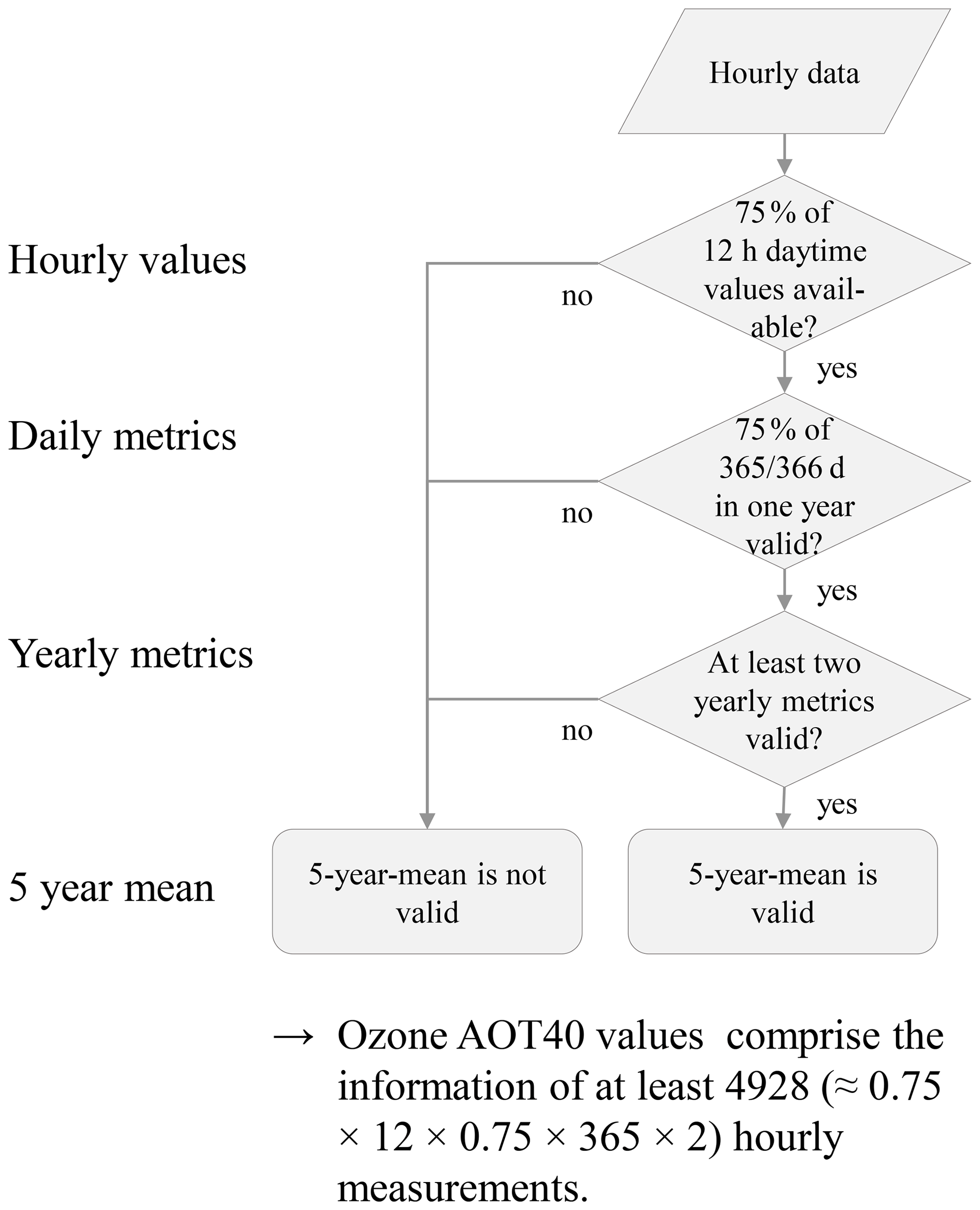
The data capture criteria applied in this work ensure robustness of the ozone metrics. Data capture criteria of hourly to annual metrics are applied through the JOIN web service (https://join.fz-juelich.de/, last access: 21 June 2021), as described in Schultz et al. (2017). The 5-year mean and its data capture criterion were applied in this work. One exception is the average value metric which does not have a data capture criterion in JOIN. Here we have verified that more than 2200 hourly values are processed to calculate the metric and that the average hourly data capture of all stations is above 50 %. The flowchart in Fig. B1 shows an example data capture criterion as applied in the AQ-Bench dataset. All data capture criteria are summarized in Table 2 of this work.
Some data from TOAR–JOIN were modified in order to make them more understandable and user-friendly.
-
HTAP region was updated according to the number code (see Table C1).
-
Climatic zone was updated according to the number code (see Table C2).
-
The variable type was harmonized, as there are some types which appear only once or twice. These types were replaced with the category they go best with:
-
The types agricultural, commercial, other-agricultural and other-marine were replaced with other.
-
The type rural was replaced with background.
-
The type urban was replaced with unknown.
Five types remain: background, industrial, traffic, other and unknown.
-
-
The variable type_of_area was harmonized in the same way as type:
-
The types alpine grasslands, background, forest and marine were replaced with unknown.
-
The types rural-nearcity and rural-regional were replaced with rural.
-
The type rural-remote was replaced with remote.
-
The type Urban was replaced with urban.
Five types of area remain: rural, urban, suburban, remote and unknown.
-
-
The station with ID 4587 was eliminated because it was a remote background station in Romania which reported an o3_average value that was one of the highest of all stations (65.5899 ppb), and it had low data coverage. We suspect its values are faulty.
-
The station with ID 4589 was eliminated because it reported a max_population_density_5km of ca. 1×10⁶ km−2 which we suspect is faulty.
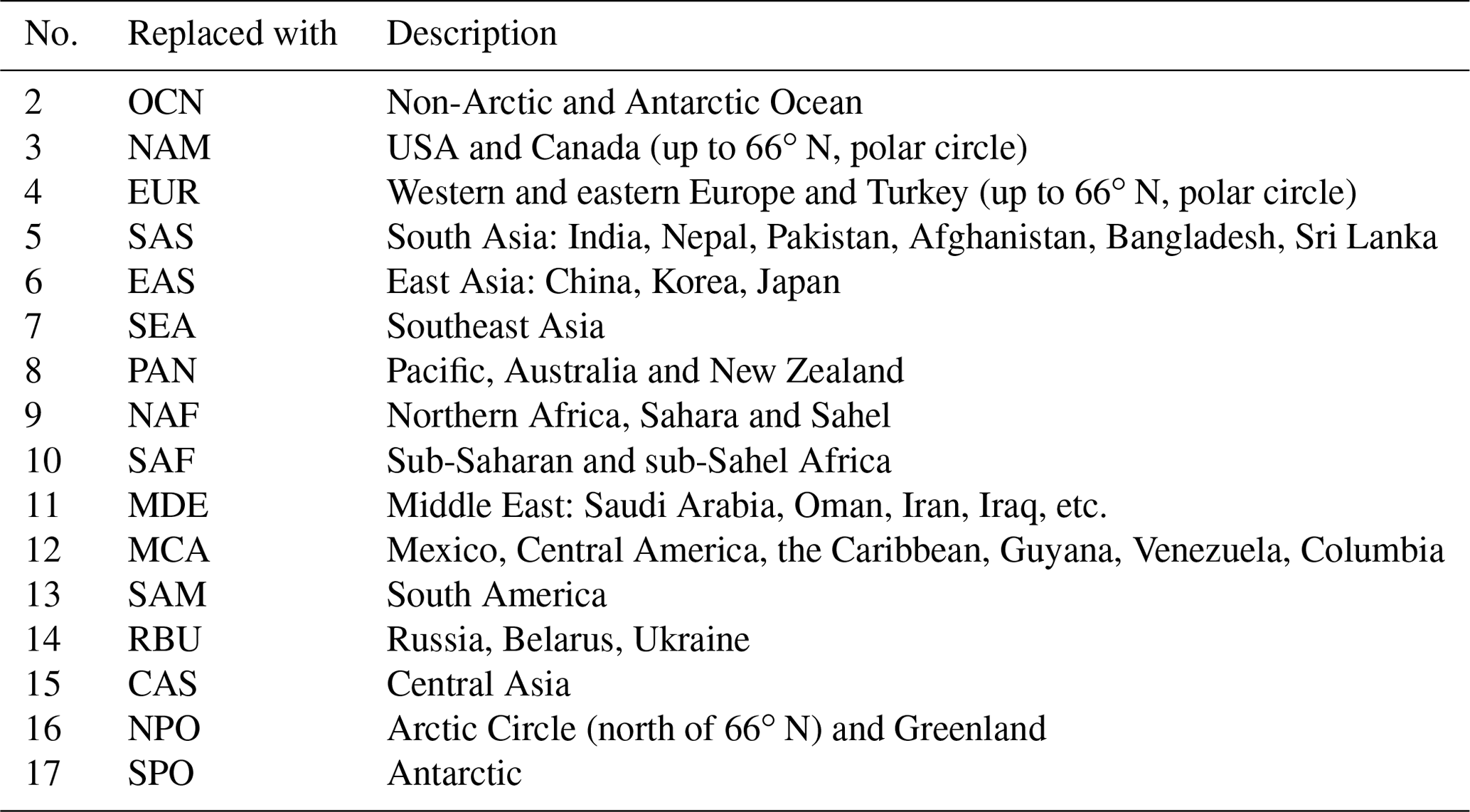
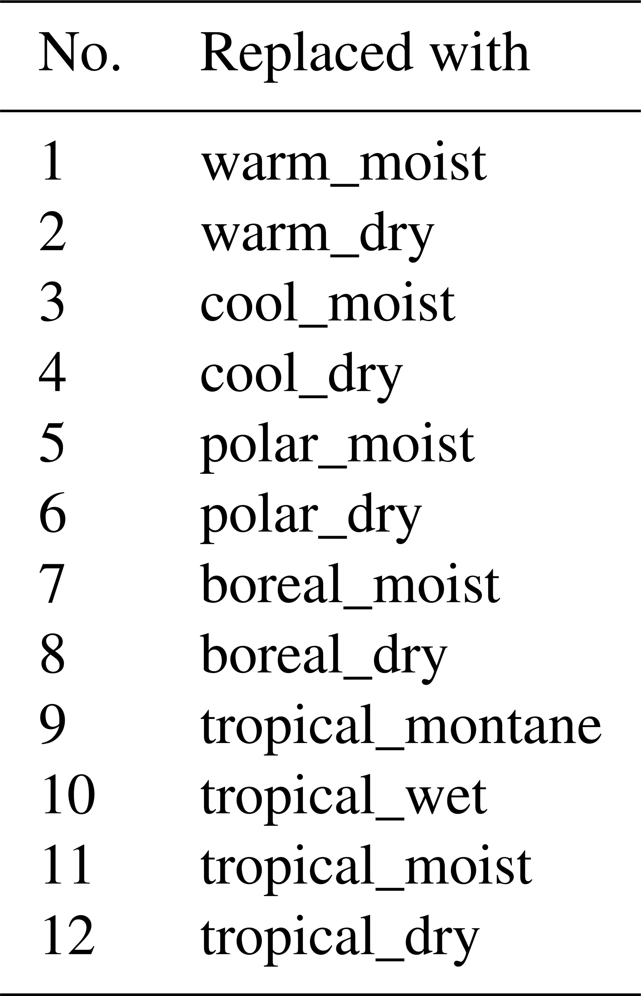
Table D1Hyperparameters for the neural network training in Sect. 5.3. They are determined from empirical studies and random search.
CB and TS prepared the dataset, developed the software and conducted the baseline experiments. CB, SS and TS prepared the initial manuscript draft. RR and MGS reviewed and edited the manuscript. All authors read and approved the manuscript. RR and MGS supervised the project. CB coordinated the project.
Martin G. Schultz is a topic editor of the ESSD journal.
Publisher's note: Copernicus Publications remains neutral with regard to jurisdictional claims in published maps and institutional affiliations.
This article is part of the special issue “Benchmark datasets and machine learning algorithms for Earth system science data (ESSD/GMD inter-journal SI)”. It is not associated with a conference.
The authors gratefully acknowledge the computing resources granted by the Jülich Supercomputing Centre (JSC). The graphical abstract of this paper was designed with icons from Flaticon (https://www.flaticon.com/, last access: 21 June 2021). We gratefully acknowledge the comments and suggestions of the two anonymous reviewers and the topical editor.
This research has been supported by the European Research Council, H2020 Research Infrastructures (IntelliAQ (grant no. ERC-2017-ADG#787576)) and the Helmholtz-Gemeinschaft (Supercomputing and Big Data of the Helmholtz Association's research field Key Technologies).
This paper was edited by David Carlson and reviewed by two anonymous referees.
Amante, C. and Eakins, B. W.: ETOPO1 arc-minute global relief model: procedures, data sources and analysis, Tech. rep., NOAA National Geophysical Data Center, available at: https://repository.library.noaa.gov/view/noaa/1163/noaa_1163_DS1.pdf (last access: 21 June 2021), 2009. a
Amodei, D., Ananthanarayanan, S., Anubhai, R., Bai, J., Battenberg, E., Case, C., Casper, J., Catanzaro, B., Cheng, Q., Chen, G., Chen, J., Chen, J., Chen, Z., Chrzanowski, M., Coates, A., Diamos, G., Ding, K., Du, N., Elsen, E., Engel, J., Fang, W., Fan, L., Fougner, C., Gao, L., Gong, C., Hannun, A., Han, T., Johannes, L., Jiang, B., Ju, C., Jun, B., LeGresley, P., Lin, L., Liu, J., Liu, Y., Li, W., Li, X., Ma, D., Narang, S., Ng, A., Ozair, S., Peng, Y., Prenger, R., Qian, S., Quan, Z., Raiman, J., Rao, V., Satheesh, S., Seetapun, D., Sengupta, S., Srinet, K., Sriram, A., Tang, H., Tang, L., Wang, C., Wang, J., Wang, K., Wang, Y., Wang, Z., Wang, Z., Wu, S., Wei, L., Xiao, B., Xie, W., Xie, Y., Yogatama, D., Yuan, B., Zhan, J., and Zhu, Z.: Deep Speech 2: End-to-End Speech Recognition in English and Mandarin, arXiv [preprint], arXiv:1512.02595, pp. 173–182, 8 December 2015. a
Benkovitz, C. M., Scholtz, M. T., Pacyna, J., Tarrasón, L., Dignon, J., Voldner, E. C., Spiro, P. A., Logan, J. A., and Graedel, T.: Global gridded inventories of anthropogenic emissions of sulfur and nitrogen, J. Geophys. Res.-Atmos., 101, 29239–29253, https://doi.org/10.1029/96JD00126, 1996. a
Betancourt, C., Stomberg, T., Stadtler, S., Roscher, R., and Schultz, M. G.: AQ-Bench, B2SHARE [data set], http://doi.org/10.23728/b2share.30d42b5a87344e82855a486bf2123e9f, 2020. a, b, c
Betancourt, C., Stadtler, S., and Stomberg, T.: AQ-Bench Git repository, GitLab – JSC [data set], available at: https://gitlab.version.fz-juelich.de/esde/machine-learning/aq-bench, last access: 21 June 2021. a, b, c
Brasseur, G., Orlando, J. J., and Tyndall, G. S. (Eds.): Atmospheric chemistry and global change, 3 edn., Oxford University Press, Oxford, UK, 1999. a
Breiman, L.: Random forests, Mach. Learn., 45, 5–32, https://doi.org/10.1023/A:1010933404324, 2001. a
Caselli, M., Trizio, L., de Gennaro, G., and Ielpo, P.: A Simple Feedforward Neural Network for the PM10 Forecasting: Comparison with a Radial Basis Function Network and a Multivariate Linear Regression Model, Water Air Soil Poll., 201, 365–377, https://doi.org/10.1007/s11270-008-9950-2, 2009. a
Chang, K.-L., Petropavlovskikh, I., Copper, O. R., Schultz, M. G., and Wang, T.: Regional trend analysis of surface ozone observations from monitoring networks in eastern North America, Europe and East Asia, Elem. Sci. Anth., 5, 50, https://doi.org/10.1525/elementa.243, 2017. a, b
Chollet, F. et al.: Keras, available at: https://keras.io (last access: 21 June 2021), 2015. a
CIESIN: Gridded Population of the World, Version 3 (GPWv3): Population Count Grid, Center for International Earth Science Information Network – CIESIN – Columbia University, United Nations Food and Agriculture Programme – FAO, and Centro Internacional de Agricultura Tropical – CIAT, Palisades, NY: NASA Socioeconomic Data and Applications Center (SEDAC), https://doi.org/10.7927/H4639MPP, 2005. a
Comrie, A. C.: Comparing Neural Networks and Regression Models for Ozone Forecasting, J. Air Waste Manage., 47, 653–663, https://doi.org/10.1080/10473289.1997.10463925, 1997. a
Cooper, O. R., Parrish, D. D., Ziemke, J., Balashov, N. V., Cupeiro, M., Galbally, I. E., Gilge, S., Horowitz, L., Jensen, N. R., Lamarque, J.-F., Naik, V., Oltmans, S. J., Schwab, J., Shindell, D. T., Thompson, A. M., Thouret, V., Wang, Y., and Zbinden, R. M.: Global distribution and trends of tropospheric ozone: An observation-based review, Elementa: Science of the Anthropocene, 2, 29, https://doi.org/10.12952/journal.elementa.000029, 2014. a
Deng, J., Dong, W., Socher, R., Li, L.-J., Li, K., and Fei-Fei, L.: ImageNet: A Large-Scale Hierarchical Image Database, in: 2009 IEEE Conference on Computer Vision and Pattern Recognition, Miami, FL, USA, 20–25 June 2009, pp. 248–255, https://doi.org/10.1109/CVPR.2009.5206848, 2009. a
Duboue, P.: The Art of Feature Engineering: Essentials for Machine Learning, 1 edn., Cambridge University Press, Cambridge, UK, https://doi.org/10.1017/9781108671682, 2020. a
Ebert-Uphoff, I., Thompson, D. R., Demir, I., Gel, Y. R., Karpatne, A., Guereque, M., Kumar, V., Cabral-Cano, E., and Smyth, P.: A vision for the development of benchmarks to bridge geoscience and data science, in: Proceedings of the 7th International Workshop on Climate Informatics, Boulder, CL, USA, 20–22 September 2017, 2017. a, b
Elkamel, A., Abdul-Wahab, S., Bouhamra, W., and Alper, E.: Measurement and prediction of ozone levels around a heavily industrialized area: a neural network approach, Adv. Environ. Res., 5, 47–59, https://doi.org/10.1016/S1093-0191(00)00042-3, 2001. a
Emberson, L., Ashmore, M., Cambridge, H., Simpson, D., and Tuovinen, J.-P.: Modelling stomatal ozone flux across Europe, Environ. Pollut., 109, 403–413, https://doi.org/10.1016/S0269-7491(00)00043-9, 2000. a
European Union: Directive 2008/50/EC of the European Parliament and of the Council of 21 May 2008 on ambient air quality and cleaner air for Europe, Official Journal of the European Union, OJ L, 1–44, available at: http://data.europa.eu/eli/dir/2008/50/oj (last access: 21 June 2021), 2008. a, b
Field, R., Goldstone, M., Lester, J., and Perry, R.: The sources and behaviour of tropospheric anthropogenic volatile hydrocarbons, Atmos. Environ. A-Gen., 26, 2983–2996, https://doi.org/10.1016/0960-1686(92)90290-2, 1992. a
Fleming, Z. L., Doherty, R. M., Von Schneidemesser, E., Malley, C. S., Cooper, O. R., Pinto, J. P., Colette, A., Xu, X., Simpson, D., Schultz, M. G., Lefohn, A. S., Hamad, S., Moolla, R., Solberg, S., and Feng, Z.: Tropospheric Ozone Assessment Report: Present-day ozone distribution and trends relevant to human health, Elem. Sci. Anth., 6, 12, https://doi.org/10.1525/elementa.273, 2018. a
Gaudel, A., Cooper, O. R., Ancellet, G., Barret, B., Boynard, A., Burrows, J. P., Clerbaux, C., Coheur, P. F., Cuesta, J., Cuevas, E., Doniki, S., Dufour, G., Ebojie, F., Foret, G., Garcia, O., Granados Muños, M. J., Hannigan, J. W., Hase, F., Huang, G., Hassler, B., Hurtmans, D., Jaffe, D., Jones, N., Kalabokas, P., Kerridge, B., Kulawik, S. S., Latter, B., Leblanc, T., Le Flochmoën, E., Lin, W., Liu, J., Liu, X., Mahieu, E., McClure-Begley, A., Neu, J. L., Osman, M., Palm, M., Petetin, H., Petropavlovskikh, I., Querel, R., Rahpoe, N., Rozanov, A., Schultz, M. G., Schwab, J., Siddans, R., Smale, D., Steinbacher, M., Tanimoto, H., Tarasick, D. W., Thouret, V., Thompson, A. M., Trickl, T., Weatherhead, E., Wespes, C., Worden, H. M., Vigouroux, C., Xu, X., Zeng, G., and Ziemke, J.: Tropospheric Ozone Assessment Report: Present-day distribution and trends of tropospheric ozone relevant to climate and global atmospheric chemistry model evaluation, Elem. Sci. Anth., 6, 39, https://doi.org/10.1525/elementa.291, 2018. a
Goodfellow, I., Bengio, Y., Courville, A., and Bengio, Y.: Deep learning, 1 edn., MIT press Cambridge, Cambridge, UK, 2016. a
He, H. and Garcia, E. A.: Learning from Imbalanced Data, IEEE Transactions on Knowledge and Data Engineering, 21, 1263–1284, https://doi.org/10.1109/TKDE.2008.239, 2009. a
Jacob, D. J.: Heterogeneous chemistry and tropospheric ozone, Atmos. Environ., 34, 2131–2159, https://doi.org/10.1016/S1352-2310(99)00462-8, 2000. a
Janssens-Maenhout, G., Crippa, M., Guizzardi, D., Dentener, F., Muntean, M., Pouliot, G., Keating, T., Zhang, Q., Kurokawa, J., Wankmüller, R., Denier van der Gon, H., Kuenen, J. J. P., Klimont, Z., Frost, G., Darras, S., Koffi, B., and Li, M.: HTAP_v2.2: a mosaic of regional and global emission grid maps for 2008 and 2010 to study hemispheric transport of air pollution, Atmos. Chem. Phys., 15, 11411–11432, https://doi.org/10.5194/acp-15-11411-2015, 2015. a
Kaiser, A., Scheifinger, H., Spangl, W., Weiss, A., Gilge, S., Fricke, W., Ries, L., Cemas, D., and Jesenovec, B.: Transport of nitrogen oxides, carbon monoxide and ozone to the alpine global atmosphere watch stations Jungfraujoch (Switzerland), Zugspitze and Hohenpeißenberg (Germany), Sonnblick (Austria) and Mt. Krvavec (Slovenia), Atmos. Environ., 41, 9273–9287, https://doi.org/10.1016/j.atmosenv.2007.09.027, 2007. a
Kelp, M. M., Jacob, D. J., Kutz, J. N., Marshall, J. D., and Tessum, C. W.: Toward Stable, General Machine-Learned Models of the Atmospheric Chemical System, J. Geophys. Res.-Atmos., 125, e2020JD032759, https://doi.org/10.1029/2020JD032759, 2020. a
Kierdorf, J., Garcke, J., Behley, J., Cheeseman, T., and Roscher, R.: What Identifies a Whale by its Fluke? on the Benefit of Interpretable Machine Learning for Whale Identification, ISPRS Annals of the Photogrammetry, Remote Sensing and Spatial Information Sciences, 2, 1005–1012, 2020. a
Kleinert, F., Leufen, L. H., and Schultz, M. G.: IntelliO3-ts v1.0: a neural network approach to predict near-surface ozone concentrations in Germany, Geosci. Model Dev., 14, 1–25, https://doi.org/10.5194/gmd-14-1-2021, 2021. a
Koffi, B., Dentener, F., Janssens-Maenhout, G., Guizzardi, D., Crippa, M., Diehl, T., Galmarini, S., and Solazzo, E.: Hemispheric Transport Air Pollution (HTAP): Specification of the HTAP2 experiments – Ensuring harmonized modelling, Tech. rep., EUR 28255 EN, Luxembourg: Publications Office of the European Union, 2016. a
Krizhevsky, A., Sutskever, I., and Hinton, G. E.: ImageNet Classification with Deep Convolutional Neural Networks, in: Advances in Neural Information Processing Systems 25: 26th Annual Conference on Neural Information Processing Systems 2012. Proceedings of a meeting held December 3–6, 2012, Lake Tahoe, Nevada, United States, https://doi.org/10.1145/3065386, pp. 1097–1105, 2012. a
Krotkov, N. A., McLinden, C. A., Li, C., Lamsal, L. N., Celarier, E. A., Marchenko, S. V., Swartz, W. H., Bucsela, E. J., Joiner, J., Duncan, B. N., Boersma, K. F., Veefkind, J. P., Levelt, P. F., Fioletov, V. E., Dickerson, R. R., He, H., Lu, Z., and Streets, D. G.: Aura OMI observations of regional SO2 and NO2 pollution changes from 2005 to 2015, Atmos. Chem. Phys., 16, 4605–4629, https://doi.org/10.5194/acp-16-4605-2016, 2016. a
LeCun, Y., Cortes, C., and Burges, C. J.: MNIST handwritten digit database, available at: http://yann.lecun.com/exdb/mnist/ (last access: 21 June 2021), 2010. a
Lefohn, A. S., Malley, C. S., Smith, L., Wells, B., Hazucha, M., Simon, H., Naik, V., Mills, G., Schultz, M. G., Paoletti, E., De Marco, A., Xu, X., Zhang, L., Wang, T., Neufeld, H. S., Musselman, R. C., Tarasick, D., Brauer, M., Feng, Z., Tang, H., Kobayashi, K., Sicard, P., Solberg, S., and Gerosa, G.: Tropospheric ozone assessment report: Global ozone metrics for climate change, human health, and crop/ecosystem research, Elem. Sci. Anth., 6, 27, https://doi.org/10.1525/elementa.279, 2018. a, b
Luhar, A. K., Woodhouse, M. T., and Galbally, I. E.: A revised global ozone dry deposition estimate based on a new two-layer parameterisation for air–sea exchange and the multi-year MACC composition reanalysis, Atmos. Chem. Phys., 18, 4329–4348, https://doi.org/10.5194/acp-18-4329-2018, 2018. a
Mills, G., Hayes, F., Simpson, D., Emberson, L., Norris, D., Harmens, H., and Büker, P.: Evidence of widespread effects of ozone on crops and (semi-) natural vegetation in Europe (1990–2006) in relation to AOT40-and flux-based risk maps, Glob. Change Biol., 17, 592–613, 2011. a
Mills, G., Pleijel, H., Malley, C. S., Sinha, B., Cooper, O. R., Schultz, M. G., Neufeld, H. S., Simpson, D., Sharps, K., Feng, Z., Gerosa, G., Harmens, H., Kobayashi, K., Saxena, P., Paoletti, E., Sinha, V., and Xu, X.: Tropospheric Ozone Assessment Report: Present-day tropospheric ozone distribution and trends relevant to vegetation, Elem. Sci. Anth., 6, 47, https://doi.org/10.1525/elementa.302, 2018. a
Monks, P. S., Archibald, A. T., Colette, A., Cooper, O., Coyle, M., Derwent, R., Fowler, D., Granier, C., Law, K. S., Mills, G. E., Stevenson, D. S., Tarasova, O., Thouret, V., von Schneidemesser, E., Sommariva, R., Wild, O., and Williams, M. L.: Tropospheric ozone and its precursors from the urban to the global scale from air quality to short-lived climate forcer, Atmos. Chem. Phys., 15, 8889–8973, https://doi.org/10.5194/acp-15-8889-2015, 2015. a
Pedregosa, F., Varoquaux, G., Gramfort, A., Michel, V., Thirion, B., Grisel, O., Blondel, M., Prettenhofer, P., Weiss, R., Dubourg, V., Vanderplas, J., Passos, A., Cournapeau, D., Brucher, M., Perrot, M., and Duchesnay, E.: Scikit-learn: Machine Learning in Python, J. Mach. Learn. Res., 12, 2825–2830, available at: https://www.jmlr.org/papers/volume12/pedregosa11a/pedregosa11a.pdf (last access: 21 June 2021), 2011. a
Porter, W. C., Heald, C. L., Cooley, D., and Russell, B.: Investigating the observed sensitivities of air-quality extremes to meteorological drivers via quantile regression, Atmos. Chem. Phys., 15, 10349–10366, https://doi.org/10.5194/acp-15-10349-2015, 2015. a
Rasp, S., Dueben, P. D., Scher, S., Weyn, J. A., Mouatadid, S., and Thuerey, N.: WeatherBench: A benchmark dataset for data-driven weather forecasting, J. Adv. Model. Earth Sy., 12, e2020MS002203, https://doi.org/10.1029/2020MS002203, 2020. a
Roscher, R., Bohn, B., Duarte, M. F., and Garcke, J.: Explainable machine learning for scientific insights and discoveries, IEEE Access, 8, 42200–42216, https://doi.org/10.1109/ACCESS.2020.2976199, 2020. a
Sayeed, A., Choi, Y., Eslami, E., Lops, Y., Roy, A., and Jung, J.: Using a deep convolutional neural network to predict 2017 ozone concentrations, 24 hours in advance, Neural Networks, 121, 396–408, https://doi.org/10.1016/j.neunet.2019.09.033, 2020. a
Schmitz, S., Towers, S., Villena, G., Caseiro, A., Wegener, R., Klemp, D., Langer, I., Meier, F., and von Schneidemesser, E.: Unraveling a black box: An open-source methodology for the field calibration of small air quality sensors, Atmos. Meas. Tech. Discuss. [preprint], https://doi.org/10.5194/amt-2020-489, in review, 2021. a
Schraudner, M., Langebartels, C., and Sandermann, H.: Changes in the biochemical status of plant cells induced by the environmental pollutant ozone, Physiol. Plantarum, 100, 274–280, https://doi.org/10.1111/j.1399-3054.1997.tb04783.x, 1997. a
Schultz, M. G., Jacob, D. J., Wang, Y., Logan, J. A., Atlas, E. L., Blake, D. R., Blake, N. J., Bradshaw, J. D., Browell, E. V., Fenn, M. A., Flocke F., Gregory, G. L., Heikes, B. G., Sachse, G. W., Sandholm, S. T., Shetter, R. E., Singh, H. B., and Talbot, R. W.: On the origin of tropospheric ozone and NOx over the tropical South Pacific, J. Geophys. Res.-Atmos., 104, 5829–5843, https://doi.org/10.1029/98JD02309, 1999. a
Schultz, M. G., Schröder, S., Lyapina, O., Cooper, O., Galbally, I., Petropavlovskikh, I., Von Schneidemesser, E., Tanimoto, H., Elshorbany, Y., Naja, M., Seguel, R., Dauert, U., Eckhardt, P., Feigenspahn, S., Fiebig, M., Hjellbrekke, A.-G., Hong, Y.-D., Christian Kjeld, P., Koide, H., Lear, G., Tarasick, D., Ueno, M., Wallasch, M., Baumgardner, D., Chuang, M.-T., Gillett, R., Lee, M., Molloy, S., Moolla, R., Wang, T., Sharps, K., Adame, J. A., Ancellet, G., Apadula, F., Artaxo, P., Barlasina, M., Bogucka, M., Bonasoni, P., Chang, L., Colomb, A., Cuevas, E., Cupeiro, M., Degorska, A., Ding, A., Fröhlich, M., Frolova, M., Gadhavi, H., Gheusi, F., Gilge, S., Gonzalez, M. Y., Gros, V., Hamad, S. H., Helmig, D., Henriques, D., Hermansen, O., Holla, R., Huber, J., Im, U., Jaffe, D. A., Komala, N., Kubistin, D., Lam, K.-S., Laurila, T., Lee, H., Levy, I., Mazzoleni, C., Mazzoleni, L., McClure-Begley, A., Mohamad, M., Murovic, M., Navarro-Comas, M., Nicodim, F., Parrish, D., Read, K. A., Reid, N., Ries, L., Saxena, P., Schwab, J. J., Scorgie, Y., Senik, I., Simmonds, P., Sinha, V., Skorokhod, A., Spain, G., Spangl, W., Spoor, R., Springston, S. R., Steer, K., Steinbacher, M., Suharguniyawan, E., Torre, P., Trickl, T., Weili, L., Weller, R., Xu, X., Xue, L., and Zhiqiang, M.: Tropospheric Ozone Assessment Report: Database and Metrics Data of Global Surface Ozone Observations, Elem. Sci. Anth., 5, 58, https://doi.org/10.1525/elementa.244, 2017. a, b, c, d, e, f, g, h, i
Schultz M. G., Betancourt C., Gong B., Kleinert F., Langguth M., Leufen L. H., Mozaffari A., and Stadtler S.: Can deep learning beat numerical weather prediction?, Philos. T. R. Soc. A., 379, 20200097, https://doi.org/10.1098/rsta.2020.0097, 2021. a, b
Sillman, S.: The relation between ozone, NOx and hydrocarbons in urban and polluted rural environments, Atmos. Environ., 33, 1821–1845, 1999. a
Silva, S. J., Heald, C. L., Ravela, S., Mammarella, I., and Munger, J. W.: A Deep Learning Parameterization for Ozone Dry Deposition Velocities, Geophys. Res. Lett., 46, 983–989, https://doi.org/10.1029/2018GL081049, 2019. a
Silver, D., Huang, A., Maddison, C. J., Guez, A., Sifre, L., van den Driessche, G., Schrittwieser, J., Antonoglou, I., Panneershelvam, V., Lanctot, M., Dieleman, S., Grewe, D., Nham, J., Kalchbrenner, N., Sutskever, I., Lillicrap, T., Leach, M., Kavukcuoglu, K., Graepel, T., and Hassabis, D.: Mastering the game of Go with deep neural networks and tree search, Nature, 529, 484–489, https://doi.org/10.1038/nature16961, 2016. a
Simpson, D., Winiwarter, W., Börjesson, G., Cinderby, S., Ferreiro, A., Guenther, A., Hewitt, C. N., Janson, R., Khalil, M. A. K., Owen, S., Pierce, T. E., Puxbaum, H., Shearer, M., Skiba, U., Steinbrecher, R., Tarrasón, L., and Öquist, M. G.: Inventorying emissions from nature in Europe, J. Geophys. Res.-Atmos., 104, 8113–8152, https://doi.org/10.1029/98JD02747, 1999. a
Tarasick, D., Galbally, I. E., Cooper, O. R., Schultz, M. G., Ancellet, G., Leblanc, T., Wallington, T. J., Ziemke, J., Liu, X., Steinbacher, M., Staehelin, J., Vigouroux, C., Hannigan, J. W., García, O., Foret, G., Zanis, P., Weatherhead, E., Petropavlovskikh, I., Worden, H., Osman, M., Liu, J., Chang, K.-L., Gaudel, A., Lin, M., Granados-Muñoz, M., Thompson, A. M., Oltmans, S. J., Cuesta, J., Dufour, G., Thouret, V., Hassler, B., Trickl, T., and Neu, J. L.: Tropospheric Ozone Assessment Report: Tropospheric ozone from 1877 to 2016, observed levels, trends and uncertainties, Elem. Sci. Anth., 7, 39, https://doi.org/10.1525/elementa.376, 2019. a
Veldkamp, E. and Keller, M.: Fertilizer-induced nitric oxide emissions from agricultural soils, Nutr. Cycl. Agroecosys., 48, 69–77, https://doi.org/10.1023/A:1009725319290, 1997. a
Wagstaff, K.: Machine learning that matters, arXiv [preprint], arXiv:1206.4656, 18 June 2012. a
Wallace, J. and Hobbs, P.: Atmospheric Science: An Introductory Survey: Second Edition, vol. 92 of International Geophysics Series, Elsevier Academic Press, Burlington, MA, USA, 2006. a, b
Wang, S., Ma, Y., Wang, Z., Wang, L., Chi, X., Ding, A., Yao, M., Li, Y., Li, Q., Wu, M., Zhang, L., Xiao, Y., and Zhang, Y.: Mobile monitoring of urban air quality at high spatial resolution by low-cost sensors: impacts of COVID-19 pandemic lockdown, Atmos. Chem. Phys., 21, 7199–7215, https://doi.org/10.5194/acp-21-7199-2021, 2021. a
Wang, Y., Choi, Y., Zeng, T., Davis, D., Buhr, M., Huey, L. G., and Neff, W.: Assessing the photochemical impact of snow NOx emissions over Antarctica during ANTCI 2003, Atmos. Environ., 41, 3944–3958, https://doi.org/10.1016/j.atmosenv.2007.01.056, 2007. a
Wessel, P., Luis, J. F., Uieda, L., Scharroo, R., Wobbe, F., Smith, W. H. F., and Tian, D.: The Generic Mapping Tools Version 6, Geochem. Geophy. Geosy., 20, 5556–5564, https://doi.org/10.1029/2019GC008515, 2019. a
Wilkinson, M. D., Dumontier, M., Aalbersberg, I. J., Appleton, G., Axton, M., Baak, A., Blomberg, N., Boiten, J.-W., da Silva Santos, L. B., Bourne, P. E., Bouwman, J., Brookes, A. J., Clark, T., Crosas, M., Dillo, I., Dumon, O., Edmunds, S., Evelo, C. T., Finkers, R., Gonzalez-Beltran, A., Gray, A. J., Groth, P., Goble, C., Grethe, J. S., Heringa, J., ’t Hoen, P. A. C., Hooft, R., Kuhn, T., Kok, R., Kok, J., Lusher, S. J., Martone, M. E., Mons, A., Packer, A. L., Persson, B., Rocca-Serra, P., Roos, M., van Schaik, R., Sansone, S.-A., Schultes, E., Sengstag, T., Slater, T., Strawn, G., Swertz, M. A., Thompson, M., van der Lei, J., van Mulligen, E., Velterop, J., Waagmeester, A., Wittenburg, P., Wolstencroft, K., Zhao, J., and Mons, B.: The FAIR Guiding Principles for scientific data management and stewardship, Scientific Data, 3, 160018, https://doi.org/10.1038/sdata.2016.18, 2016. a
Wise, E. K. and Comrie, A. C.: Extending the Kolmogorov–Zurbenko filter: application to ozone, particulate matter, and meteorological trends, J. Air Waste Manage., 55, 1208–1216, https://doi.org/10.1080/10473289.2005.10464718, 2005. a
Xu, J., Ma, J. Z., Zhang, X. L., Xu, X. B., Xu, X. F., Lin, W. L., Wang, Y., Meng, W., and Ma, Z. Q.: Measurements of ozone and its precursors in Beijing during summertime: impact of urban plumes on ozone pollution in downwind rural areas, Atmos. Chem. Phys., 11, 12241–12252, https://doi.org/10.5194/acp-11-12241-2011, 2011. a
Xu, X., Lin, W., Xu, W., Jin, J., Wang, Y., Zhang, G., Zhang, X., Ma, Z., Dong, Y., Ma, Q., Yu, D., Li, Z., Wang, D., and Zhao, H.: Tropospheric Ozone Assessment Report: Long-term changes of regional ozone in China: implications for human health and ecosystem impacts, Elem. Sci. Anth., 8, 13, https://doi.org/10.1525/elementa.409, 2020. a
Yi, J. and Prybutok, V. R.: A neural network model forecasting for prediction of daily maximum ozone concentration in an industrialized urban area, Environ. Pollut., 92, 349–357, 1996. a
Young, P. J., Naik, V., Fiore, A. M., Gaudel, A., Guo, J., Lin, M. Y., Neu, J. L., Parrish, D. D., Rieder, H. E., Schnell, J. L., Tilmes, S., Wild, O., Zhang, L., Ziemke, J. R., Brandt, J., Delcloo, A., Doherty, R. M., Geels, C., Hegglin, M. I., Hu, L., Im, U., Kumar, R., Luhar, A., Murray, L., Plummer, D., Rodriguez, J., Saiz-Lopez, A., Schultz, M. G., Woodhouse, M. T., and Zeng, G.: Tropospheric Ozone Assessment Report: Assessment of global-scale model performance for global and regional ozone distributions, variability, and trends, Elem. Sci. Anth., 6, 10, https://doi.org/10.1525/elementa.265, 2018. a
Zhang, Y. and Yang, Q.: A survey on multi-task learning, arXiv [preprint], arXiv:1707.08114, 25 July 2017. a
https://join.fz-juelich.de/ (last access: 21 June 2021).
https://join.fz-juelich.de/services/rest/surfacedata/ (last access: 21 June 2021).
https://doi.org/10.1594/PANGAEA.876108 (last access: 21 June 2021).
https://join.fz-juelich.de/ (last access: 21 June 2021).
- Abstract
- Introduction
- What factors influence ozone?
- TOAR data products
- AQ-Bench dataset description
- Validating AQ-Bench via machine learning
- Discussion
- Data and code availability
- Conclusions
- Appendix A: Technical details on the station metadata of the AQ-Bench dataset
- Appendix B: Data capture criteria
- Appendix C: Data editing
- Appendix D: Hyperparameters for baselines
- Author contributions
- Competing interests
- Disclaimer
- Special issue statement
- Acknowledgements
- Financial support
- Review statement
- References