Carbon Monitoring System Flux Net Biosphere Exchange 2020 (CMS-Flux NBE 2020)

Here we present a global and regionally resolved terrestrial net biosphere exchange (NBE) dataset with corresponding uncertainties between 2010–2018: Carbon Monitoring System Flux Net Biosphere Exchange 2020 (CMS-Flux NBE 2020). It is estimated using the NASA Carbon Monitoring System Flux (CMS-Flux) top-down flux inversion system that assimilates column CO₂ observations from the Greenhouse Gases Observing Satellite (GOSAT) and NASA's Observing Carbon Observatory 2 (OCO-2). The regional monthly fluxes are readily accessible as tabular files, and the gridded fluxes are available in NetCDF format. The fluxes and their uncertainties are evaluated by extensively comparing the posterior CO₂ mole fractions with CO₂ observations from aircraft and the NOAA marine boundary layer reference sites. We describe the characteristics of the dataset as the global total, regional climatological mean, and regional annual fluxes and seasonal cycles. We find that the global total fluxes of the dataset agree with atmospheric CO₂ growth observed by the surface-observation network within uncertainty. Averaged between 2010 and 2018, the tropical regions range from close to neutral in tropical South America to a net source in Africa; these contrast with the extra-tropics, which are a net sink of 2.5±0.3 Gt C/year. The regional satellite-constrained NBE estimates provide a unique perspective for understanding the terrestrial biosphere carbon dynamics and monitoring changes in regional contributions to the changes of atmospheric CO₂ growth rate. The gridded and regional aggregated dataset can be accessed at https://doi.org/10.25966/4v02-c391 (Liu et al., 2020).

1 Introduction

New top-down inversion frameworks that harness satellite observations provide an important complement to global aggregated fluxes (e.g., Global Carbon Budget (GCB), Friedlingstein et al., 2019) and inversions based on surface CO₂ observations (e.g., Chevallier et al., 2010), especially over the tropics and the Southern Hemisphere (SH) where conventional surface CO₂ observations are sparse. The net biosphere exchange (NBE), which is the net carbon flux of all the land–atmosphere exchange processes except fossil fuel emissions, is far more variable and has far more uncertainty than ocean fluxes (Lovenduski and Bonan, 2017) or fossil fuel emissions (Yin et al., 2019) and is thus the focus of this dataset estimated from a top-down atmospheric CO₂ inversion of satellite column CO₂ dry-air mole fraction (X${}_{{\mathrm{CO}}_{\mathrm{2}}}$). Here, we present the global and regional NBE as a series of maps, time series, and tables and disseminate it as a public dataset for further analysis and comparison to other sources of flux information. The gridded NBE dataset and its uncertainty, air–sea fluxes, and fossil fuel emissions are also available so that users can calculate the carbon budget from a regional to global scale. Finally, we provide a comprehensive evaluation of both mean and uncertainty estimates against the CO₂ observations from independent airborne datasets and the NOAA marine boundary layer (MBL) reference sites (Conway et al., 1994).

Global top-down atmospheric CO₂ flux inversions have been historically used to estimate regional terrestrial NBE. They make uses of the spatiotemporal variability of atmospheric CO₂, which is dominated by NBE, to infer net carbon exchange at the surface (Chevallier et al., 2005; Baker et al., 2006a; Liu et al., 2014). The accuracy of the NBE from top-down flux inversions is determined by the density and accuracy of the CO₂ observations, the accuracy of modeled atmospheric transport, and knowledge of the prior uncertainties of the flux inventories.

For CO₂ flux inversions based on high precision in situ and flask observations, the measurement error is low (<0.2 ppm, parts per million) and not a significant source of error; however, these observations are limited spatially and are concentrated primarily over North America (NA) and Europe (Crowell et al., 2019). Satellite X${}_{{\mathrm{CO}}_{\mathrm{2}}}$ observations from CO₂-dedicated satellites, such as the Greenhouse Gases Observing Satellite (GOSAT) (launched in July 2009) and the Observing Carbon Observatory 2 (OCO-2) (Crisp et al., 2017), have much broader spatial coverage (O'Dell et al., 2018), which fills the observational gaps of conventional surface CO₂ observations, but they have up to an order of magnitude higher single-sounding uncertainty and potential systematic errors compared to the in situ and flask CO₂ observations. Recent progress in instrument error characterization, spectroscopy, and retrieval methods has significantly improved the accuracy and precision of the X${}_{{\mathrm{CO}}_{\mathrm{2}}}$ retrievals (O'Dell et al., 2018; Kiel et al., 2019). The single-sounding random error of X${}_{{\mathrm{CO}}_{\mathrm{2}}}$ from OCO-2 is ∼1.0 ppm (Kulawik et al., 2019). A recent study by Byrne et al. (2020) shows less than a 0.5 ppm difference between posterior X${}_{{\mathrm{CO}}_{\mathrm{2}}}$ constrained by a recent dataset, ACOS-GOSAT b7 X${}_{{\mathrm{CO}}_{\mathrm{2}}}$ retrievals, and those constrained by conventional surface CO₂ observations. Chevallier et al. (2019) also showed that an OCO-2-based flux inversion had similar performance to surface CO₂-based flux inversions when comparing posterior CO₂ mole fractions to aircraft CO₂ in the free troposphere. Results from these studies show that systematic uncertainties in CO₂ retrievals from satellites are comparable to, or smaller than, other uncertainty sources in atmospheric inversions (e.g., transport).

A newly developed biogeochemical model–data fusion system, CARDAMOM, made progress in producing NBE uncertainties, along with mean values that are consistent with a variety of observations assimilated through a Markov chain Monte Carlo (MCMC) method (Bloom et al., 2016, 2020). Transport model errors in general have also been reduced relative to earlier transport model intercomparison efforts, such as TransCom 3 (Gurney et al., 2004; Gaubert et al., 2019). Advancements in satellite retrieval, transport, and prior terrestrial biosphere modeling have led to more mature inversions constrained by satellite X${}_{{\mathrm{CO}}_{\mathrm{2}}}$ observations.

Two satellites, GOSAT and OCO-2, have now produced more than 10 years of observations. Here we harness the NASA Carbon Monitoring System Flux (CMS-Flux) inversion framework (Liu et al., 2014, 2017, 2018; Bowman et al., 2017) to generate an NBE product – Carbon Monitoring System Flux Net Biosphere Exchange 2020 (CMS-Flux NBE 2020) – by assimilating both GOSAT and OCO-2 from 2010–2018. The dataset is the longest satellite-constrained NBE product so far. The CMS-Flux framework exploits globally available X${}_{{\mathrm{CO}}_{\mathrm{2}}}$ to infer spatially resolved total surface–atmosphere exchange. In combination with constituent fluxes, e.g., gross primary production (GPP), NBE from CMS-Flux framework has been used to assess the impacts of El Niño on terrestrial biosphere fluxes (Bowman et al., 2017; Liu et al., 2017) and the role of droughts in the North American carbon balance (Liu et al., 2018). These fluxes have furthermore been ingested into land–surface data assimilation systems to quantify heterotrophic respiration (Konings et al., 2019), evaluate structural and parametric uncertainty in carbon–climate models (Quetin et al., 2020), and inform climate dynamics (Bloom et al., 2020). We present the regional NBE and its uncertainty based on three types of regional masks: (1) latitude and continent, (2) distribution of biome types (defined by plant functional types) and continent, and (3) TransCom regions (Gurney et al., 2004).

The outline of the paper is as follows: Sect. 2 describes methods, and Sects. 3 and 4 describe the dataset and the major NBE characteristics, respectively. We extensively evaluate the posterior fluxes and uncertainties by comparing the posterior CO₂ mole fractions against aircraft observations and the NOAA MBL reference CO₂, as well as a gross primary production (GPP) product (Sect. 5). In Sect. 6, we discuss the strength and weakness as well as potential usage of the data. A summary is provided in Sect. 7, and Sect. 8 describes the dataset availability and future plan.

Figure 1 Data flow diagram with the main processing steps to generate regional net biosphere exchange (NBE). TER: total ecosystem respiration; GPP: gross primary production. The green box is the inversion system. The blue boxes are the inputs for the inversion system. The red boxes are the data outputs from the system. The black box is the evaluation step, and the gray boxes are the future additions to the product.

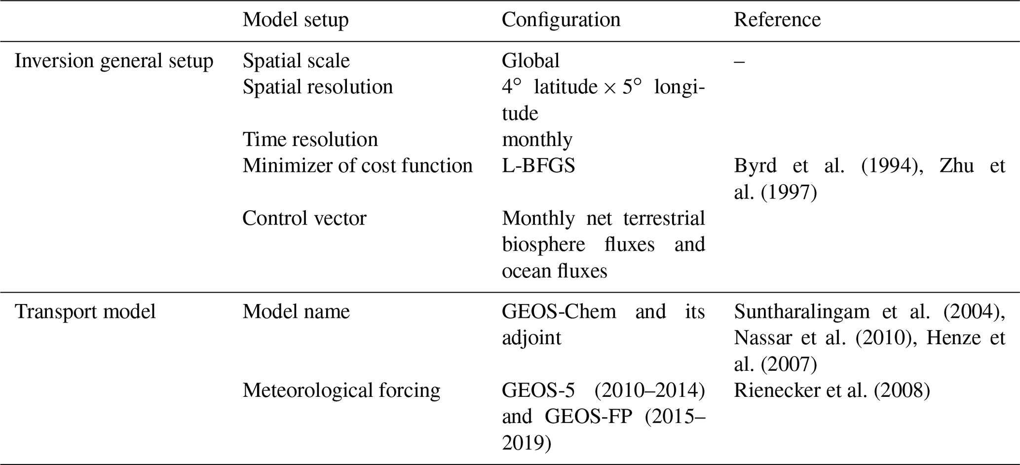
Table 1 Configurations of the CMS-Flux atmospheric inversion system.

2 Methods

2.1 CMS-Flux inversion system

The CMS-Flux framework is summarized in Fig. 1. The center of the system is the CMS-Flux inversion system, which optimizes NBE and air–sea net carbon exchanges with a 4D-Var inversion system (Liu et al., 2014). In the current system, we assume no uncertainty in fossil fuel emissions, which is a widely adopted assumption in global flux inversion systems (e.g., Crowell et al., 2019), since the uncertainty in fossil fuel emissions at regional scales is substantially less than the NBE uncertainties. The 4D-Var minimizes a cost function that includes two terms:

$$\begin{array}{}\text{(1)}& \begin{array}{rl}J\left(\mathit{x}\right)& =(\mathit{x}-{\mathit{x}}_b{)}^T{\mathbf{B}}^{-\mathrm{1}}(\mathit{x}-{\mathit{x}}^b)\\ & +(\mathit{y}-h(\mathit{x}\left){)}^T{\mathbf{R}}^{-\mathrm{1}}\right(\mathit{y}-h\left(\mathit{x}\right)).\end{array}\end{array}$$

The first term measures the differences between the optimized fluxes and the prior fluxes normalized by the prior flux error covariance B. The second term measures the differences between observations (y) and the corresponding model simulations (h(x)) normalized by the observation error covariance R. The term h(⋅) is the observation operator that calculates observation-equivalent model-simulated X${}_{{\mathrm{CO}}_{\mathrm{2}}}$. The 4D-Var uses the adjoint (i.e., the backward integration of the transport model) (Henze et al., 2007) of the GEOS-Chem transport model to calculate the sensitivity of the observations to surface fluxes. The configurations of the inversion system are summarized in Table 1. We run both the forward model and its adjoint at 4^∘ × 5^∘ spatial resolution and optimize monthly NBE and air–sea carbon fluxes at each grid point from January 2010 to December 2018. Inputs for the system include prior carbon fluxes, meteorological drivers, and the satellite X${}_{{\mathrm{CO}}_{\mathrm{2}}}$ (Fig. 1). Sect. 2.2 (Table 2) describes the prior flux and its uncertainties, and Sect. 2.3 (Table 3) describes the observations and the corresponding uncertainties.

Table 2 Description of the prior fluxes and assumed uncertainties in the inversion system.

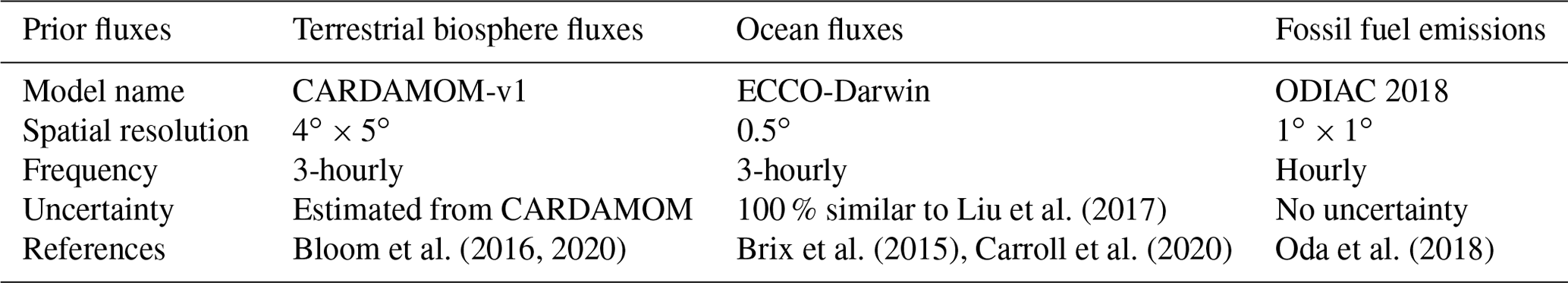
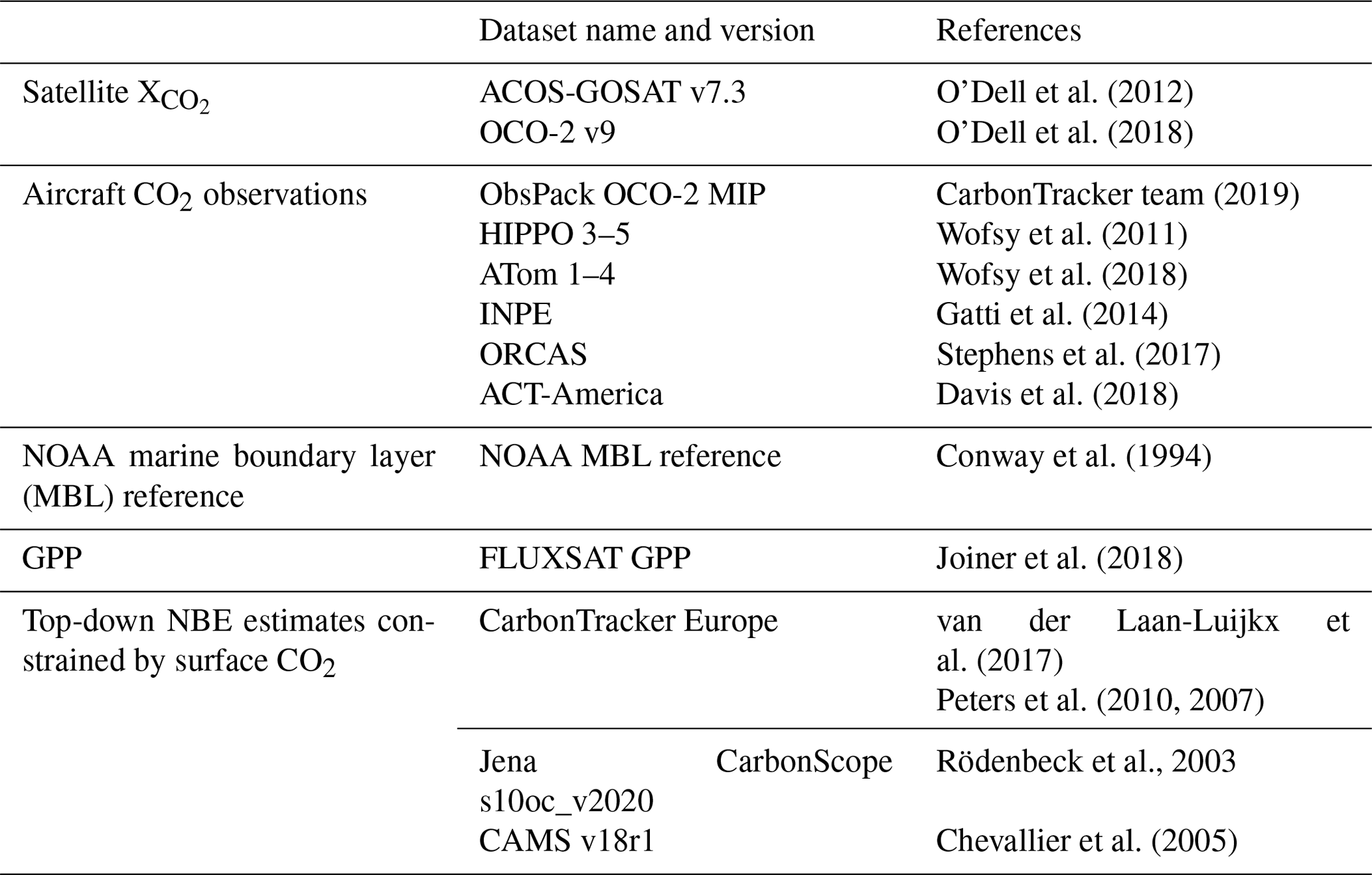
Table 3 Description of observation and evaluation dataset. Data sources are listed in Table 7.

2.2 The prior CO₂ fluxes and uncertainties

The prior CO₂ fluxes include NBE, air–sea carbon exchange, and fossil fuel emissions (see Table 2). The data sources for the prior fluxes are listed in Table 7 and provided in the gridded fluxes. Methods to generate prior ocean carbon fluxes and fossil fuel emissions are documented in Brix et al. (2015), Caroll et al. (2020), and Oda et al. (2018). The focus of this dataset is optimized terrestrial biosphere fluxes, so we briefly describe the prior terrestrial biosphere fluxes and their uncertainties.

We construct the NBE prior using the CARDAMOM framework (Bloom et al., 2016). The CARDAMOM data assimilation system explicitly represents the time-resolved uncertainties in the NBE. The prior estimates are already constrained with multiple data streams accounting for measurement uncertainties following a Bayesian approach similar to that used in the 4D-variational approach. We use the CARDAMOM setup as described by Bloom et al. (2016, 2020) resolved at monthly timescales; data constraints include Global Ozone Monitoring Experiment 2 (GOME-2) solar-induced fluorescence (Joiner et al., 2013), MODIS leaf area index (LAI), and biomass and soil carbon (details on the data assimilation are provided in Bloom et al., 2020). In addition, mean GPP and fire carbon emissions from 2010–2017 are constrained by FLUXCOM RS + METEO version 1 GPP (Tramontana et al., 2016; Jung et al., 2017) and GFEDv4.1s (Randerson et al., 2018), respectively, both assimilated with an uncertainty of 20 %. We use the Olsen and Randerson (2004) approach to downscale monthly GPP and respiration fluxes to 3-hourly timescales, based on ERA-Interim re-analysis of global radiation and surface temperature. Fire fluxes are downscaled using the GFEDv4.1 daily- and diurnal-scale factors on monthly emissions (Giglio et al., 2013). Posterior CARDAMOM NBE estimates are then summarized as NBE mean and standard deviation values.

The NBE from CARDAMOM shows net carbon uptake of 2.3 Gt C/year over the tropics and close to neutral in the extra-tropics (Fig. B1). The year-to-year variability (i.e., interannual variability, IAV) estimated from CARDAMOM is generally less than 0.1 g C/m²/d outside of the tropics (Fig. B1). Because of the weak interannual variability estimated by CARDAMOM, we use the same 2017 NBE prior for 2018.

CARDAMOM generates uncertainty along with the mean state. The relative uncertainty over the tropics is generally larger than 100 %, and the magnitude is between 50 % and 100 % over the extra-tropics (Fig. B2). We assume no correlation in the prior flux errors in either space or time. The temporal and spatial error correlation estimates can in principle be computed by CARDAMOM. We anticipate incorporating these error correlations in subsequent versions of this dataset.

2.3 Column CO₂ observations from GOSAT and OCO-2

We use the satellite-column CO₂ retrievals from the Atmospheric Carbon Observations from Space (ACOS) team for both GOSAT (version 7.3) and OCO-2 (version 9) (Table 3). The use of the same retrieval algorithm and validation strategy adopted by the ACOS team to process both GOSAT and OCO-2 spectra maximizes the consistency between these two datasets. Both GOSAT and OCO-2 satellites carry high-resolution spectrometers optimized to return high-precision measurements of reflected sunlight within CO₂ and O₂ absorption bands in the shortwave infrared (Crisp et al., 2012). Both satellites fly in a sun-synchronous orbit. GOSAT has a 13:00±0.15 h local passing time and a 3 d ground track repeat cycle. The footprint of GOSAT is ∼10.5 km in diameter in sun nadir view (Crisp et al., 2012). The daily number of soundings processed by the ACOS-GOSAT retrieval algorithm is between a few hundred to ∼2000. Further quality control and filtering reduce the ACOS-GOSAT X${}_{{\mathrm{CO}}_{\mathrm{2}}}$ retrievals to ∼100–300 daily (Fig. B5 in Liu et al., 2017). We only assimilate ACOS-GOSAT land nadir observations flagged as being good quality, which are the retrievals with quality flag equal to zero.

OCO-2 has a 13:30 local passing time and 16 d ground track repeat cycle. The nominal footprints of the OCO-2 are 1.25 km wide and ∼2.4 km along the orbit. Because of its small footprints and sampling strategy, OCO-2 has many more X${}_{{\mathrm{CO}}_{\mathrm{2}}}$ retrievals than ACOS-GOSAT. To reduce the sampling error due to the resolution differences between the transport model and OCO-2 observations, we generate super observations by aggregating the observations within ∼100 km (along the same orbit) (Liu et al., 2017). The super-obing strategy was first proposed in numerical weather prediction (NWP) to assimilate dense observations (Lorenc, 1981) and is still broadly used in NWP (e.g., Liu and Rabier, 2003). More detailed information about OCO-2 super observations can be found in Liu et al. (2017). OCO-2 has four observing modes: land nadir, land glint, ocean glint, and target. Following Liu et al. (2017), we only use land nadir observations. The super observations have more uniform spatial coverage and are more comparable to the spatial representation of ACOS-GOSAT observations and the transport model (see Fig. B5 in Liu et al., 2017).

We directly use observational uncertainty provided with ACOS-GOSAT b7.3 to represent the observation error statistics, R, in Eq. (1). The uncertainty of the OCO-2 super observations is the sum of the variability of X${}_{{\mathrm{CO}}_{\mathrm{2}}}$ used to generate each individual super observation and the mean uncertainty provided in the original OCO-2 retrievals. Kulawik et al. (2019) showed that both OCO-2 and ACOS-GOSAT bias-corrected retrievals have a mean bias of −0.1 ppm when compared with X${}_{{\mathrm{CO}}_{\mathrm{2}}}$ from the Total Carbon Column Observing Network (TCCON) (Wunch et al., 2011), indicating consistency between ACOS-GOSAT and OCO-2 retrievals. O'Dell et al. (2018) showed that the OCO-2 X${}_{{\mathrm{CO}}_{\mathrm{2}}}$ land nadir retrievals have an RMSE of ∼1.1 ppm when compared to TCCON retrievals; the differences between OCO-2 X${}_{{\mathrm{CO}}_{\mathrm{2}}}$ retrievals and surface-CO₂-constrained model simulations are well within 1.0 ppm over most of the locations in the Northern Hemisphere (NH), where most of the surface CO₂ observations are located.

The magnitude of observation errors used in R is generally above 1.0 ppm, larger than the sum of random error and biases in the observations. The ACOS-GOSAT b7.3 observations from July 2009–June 2015 are used to optimize fluxes between 2010 and 2014, and the OCO-2 X${}_{{\mathrm{CO}}_{\mathrm{2}}}$ observations from September 2014–June 2019 are used to optimize fluxes between 2015 and 2018.

The observational coverage of ACOS-GOSAT and OCO-2 is spatiotemporally dependent, with more coverage during summer than winter over the NH and more observations over midlatitudes than over the tropics (Fig. B3). The variability (i.e., standard deviation) of the annual total number of observations from 2010–2014 is within 4 % of the annual mean number for ACOS-GOSAT. Except for a data gap in 2017 caused by a malfunction of the OCO-2 instrument, the variability of the annual total number of observations between 2015 and 2018 is within 8 % of the annual mean number for OCO-2.

2.4 Uncertainty quantification

The posterior flux error covariance is the inverse Hessian, which incorporates the transport, measurement, and background errors at the 4D-Var solution (Eq. 13 in Bowman et al., 2017). Posterior flux uncertainty projected to regions can be estimated analytically based on the methods described in Fisher and Courtier (1995) and Meirink et al. (2008), using either flux singular vectors or flux increments obtained during the iterative optimization (e.g., Niwa and Fujii, 2020). In this study, we rely on a Monte Carlo approach to quantify posterior flux uncertainties following Chevallier et al. (2010) and Liu et al. (2014), which is simpler and widely used. In this approach, an ensemble of flux inversions is carried out with an ensemble of priors and simulated observations to sample the uncertainties of prior fluxes (i.e., B in Eq. 1) and observations (R in Eq. 1), respectively. The magnitude of posterior flux uncertainties is a function of assumed uncertainties in prior fluxes and observations, as well as the density of observations. Since the densities of GOSAT and OCO-2 observations are stable (Sect. 2.3) within their respective data record, we characterize the posterior flux uncertainties for 2010 and 2015 only and assume the flux uncertainties for 2011–2014 are the same as 2010 and flux uncertainties for 2016–2018 are the same as 2015.

2.5 Evaluation of posterior fluxes

Direct NBE estimates from flux towers only provide a spatial representation of roughly 1–3 km (Running et al., 1999), which is not appropriate to evaluate regional NBE from top-down flux inversions. Thus, we use two methods to indirectly evaluate the posterior NBE and its uncertainties. One is to compare annual NBE anomalies and seasonal cycle to a gross primary production (GPP) product. The other is to compare posterior CO₂ mole fractions to independent (i.e., not assimilated in the inversion) aircraft and the NOAA MBL reference observations. The second method has been broadly used to indirectly evaluate posterior fluxes from top-down flux inversions (e.g., Stephens et al., 2007; Liu and Bowman, 2016; Chevallier et al., 2019; Crowell et al., 2019). In addition to these two methods, we also compare the NBE seasonal cycles to three publicly available top-down NBE estimates that are constrained by surface CO₂ observations (Tables 3 and 7).

2.5.1 Evaluation against the independent gross primary production (GPP) product

NBE is a small residual difference between two large terms: total ecosystem respiration (TER) and GPP, plus fire. A positive NBE anomaly (i.e., less uptake from the atmosphere) has been shown to correspond to reduced GPP caused by climate anomalies (e.g., Bastos et al., 2018), and the magnitude of net uptake is proportional to GPP in most biomes observed by flux tower observations (e.g., Falk et al., 2008). Since NBE is related not only to GPP, the comparison to GPP only serves as a qualitative measure of the NBE quality. For example, we would expect the posterior NBE seasonality to be anti-correlated with GPP in the temperate and high latitudes. In this study, we use FLUXSAT GPP (Joiner et al., 2018), which is an upscaled GPP product based on flux tower GPP observations and satellite-based geometry-adjusted reflectance from the Moderate Resolution Imaging Spectroradiometer (MODIS) and solar-induced chlorophyll fluorescence observations from GOME-2 (Joiner et al., 2013). Joiner et al. (2018) show that the agreement between FLUXSAT GPP and GPP from flux towers is better than other available upscaled GPP products.

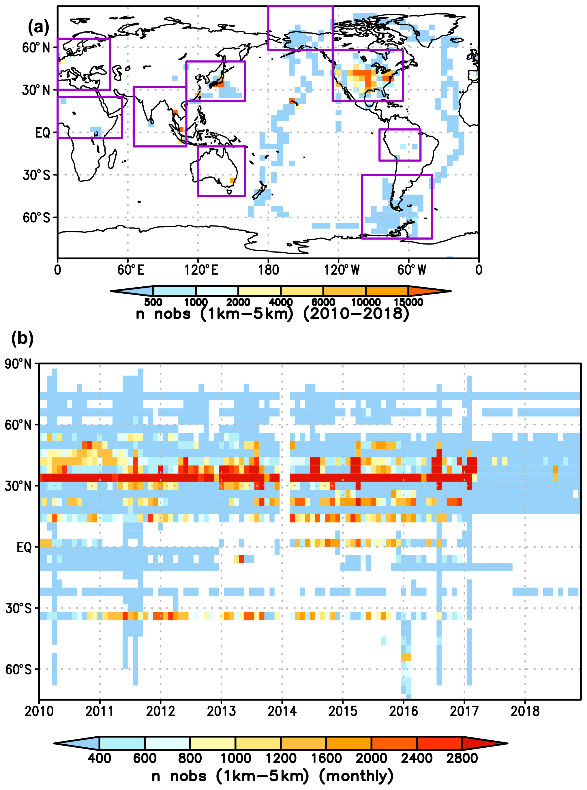
Figure 2 The spatial and temporal distributions of aircraft observations used in evaluation of posterior NBE. (a) The total number of aircraft observations between 1–5 km between 2010–2018 at each 4^∘ × 5^∘ grid point. The rectangle boxes show the range of the nine sub-regions. (b) The total number of monthly aircraft observations at each longitude as a function of time.

2.5.2 Evaluation against aircraft and the NOAA marine boundary layer (MBL) reference CO₂ observations

The aircraft observations used in this study include those published in OCO-2 MIP ObsPack in August 2019 (CarbonTracker team, 2019), which include regular vertical profiles from flask samples collected on light aircraft by NOAA (Sweeney et al., 2015) and other laboratories, regular (2- to 4-weekly) vertical profiles from the Instituto de Pesquisas Espaciais (INPE) over tropical South America (SA) (Gatti et al., 2014), and vertical profiles from the Atmospheric Tomography (ATom, Wofsy et al., 2018), HIAPER Pole-to-Pole Observations (HIPPO, Wofsy et al., 2011), the ${\mathrm{O}}_{\mathrm{2}}/{\mathrm{N}}_{\mathrm{2}}$ Ratio and CO₂ airborne Southern Ocean Study (ORCAS) (Stephens et al., 2017), and Atmospheric Carbon and Transport – America (ACT-America, Davis et al., 2018) aircraft campaigns (Table 3). Figure 2 shows the aircraft observation coverage and density between 2010 and 2018. Most of the aircraft observations are concentrated over NA. ATom had four (1–4) campaigns between August 2016 and May 2018, spanning four seasons over the Pacific and Atlantic Ocean. HIPPO had five (HIPPO 1–5) campaigns over the Pacific, but only HIPPO 3–5 occurred between 2010 and 2011. HIPPO 1–2 occurred in 2009. Based on the spatial distribution of aircraft observations, we divide the comparison into nine regions: Alaska, midlatitude NA, Europe, East Asia, South Asia, Africa, Australia, Southern Ocean, and South America (Table 4 and Fig. 2).

Table 4 Latitude and longitude ranges for seven sub-regions.

We calculate several quantities to evaluate the posterior fluxes and their uncertainty with aircraft observations. One is the monthly mean differences between posterior and aircraft CO₂ mole fractions. The second is the monthly root mean square errors (RMSEs) over each of the nine sub-regions, which is defined as

$$\begin{array}{}\text{(2)}& \text{RMSE}={\left({\displaystyle \frac{\mathrm{1}}{n}}\sum _{i=\mathrm{1}}^n(y_{\mathrm{aircraft}}^{\mathrm{o}}-y_{\mathrm{aircraft}}^b{)}_i^{\mathrm{2}}\right)}^{\frac{\mathrm{1}}{\mathrm{2}}},\end{array}$$

where $y_{\mathrm{aircraft}}^{\mathrm{o}}$ is the ith aircraft observation, $y_{\mathrm{aircraft}}^b$ is the corresponding posterior CO₂ mole fraction sampled at the ith aircraft location, and n is the number of aircraft observations over each region. The RMSE is computed over the n aircraft observations within one of the nine sub-regions. The mean differences indicate the magnitude of the mean posterior CO₂ bias, while the RMSE includes both random and systematic errors in posterior CO₂. The bias and RMSE could be due to errors in posterior fluxes, transport, and initial CO₂ concentrations. When errors in transport and initial CO₂ concentrations are smaller than the errors in the posterior fluxes, the magnitude of biases and RMSE indicates the accuracy of the posterior fluxes.

To evaluate the magnitude of posterior flux uncertainty estimates, we compare RMSE against the standard deviation of ensemble simulated aircraft observations (Eq. 3) from the Monte Carlo method (RMSE_MC). The quantity RMSE_MC can be written as

$$\begin{array}{}\text{(3)}& {\text{RMSE}}_{\mathrm{MC}}={\left[{\displaystyle \frac{\mathrm{1}}{n\mathrm{ens}}}\sum _{i\mathrm{ens}=\mathrm{1}}^{n\mathrm{ens}}\left(\right(y_{\mathrm{aircraft}}^{b\left(\text{MC}\right)}{)}_{i\mathrm{ens}}-{\overline{y}}_{\mathrm{aircraft}}^{b\left(\mathrm{MC}\right)}{)}^{\mathrm{2}}\right]}^{\frac{\mathrm{1}}{\mathrm{2}}}.\end{array}$$

The variable $(y_{\mathrm{aircraft}}^{b\left(\mathrm{MC}\right)}{)}_{i\mathrm{ens}}$ is the ith ensemble member of simulated aircraft observations from the Monte Carlo ensemble simulations, ${\overline{y}}_{\mathrm{aircraft}}^{b\left(\mathrm{MC}\right)}$ is the mean, and nens is the total number of ensemble members. For simplicity, in Eq. (3), we drop the indices for the aircraft observations used in Eq. (2). In the absence of errors in transport and initial CO₂ concentrations, when the estimated posterior flux uncertainty reflects the true posterior flux uncertainty, we show in the Appendix that

$$\begin{array}{}\text{(4)}& {\text{RMSE}}^{\mathrm{2}}={\displaystyle \frac{\mathrm{1}}{n}}\sum _{i=\mathrm{1}}^n{R}_{i,i}+{\text{RMSE}}_{\mathrm{MC}}^{\mathrm{2}},\end{array}$$

where R_aircraft is the aircraft observation error variance, which could be neglected on a regional scale.

We further calculate the ratio r between RMSE and RMSE_MC:

$$\begin{array}{}\text{(5)}& r={\displaystyle \frac{\text{RMSE}}{{\text{RMSE}}_{\mathrm{MC}}}}.\end{array}$$

A ratio close to one indicates that the posterior flux uncertainty reflects the true uncertainty in the posterior fluxes when the transport errors are small.

The presence of transport errors will make the comparison between RMSE and RMSE_MC potentially difficult to interpret. Even when RMSE_MC represents the actual uncertainty in posterior fluxes, the RMSE could be larger than RMSE_MC, since the differences between aircraft observations and model-simulated posterior mole fraction RMSE could be due to errors in both transport and the posterior fluxes, while RMSE_MC only reflects the impact of posterior flux uncertainty on simulated aircraft observations. In this study, we assume the primary sources of RMSE come from errors in posterior fluxes.

The RMSE and RMSE_MC comparison only shows differences in CO₂ space. We further calculate the sensitivity of the RMSE to the posterior flux using the GEOS-Chem adjoint. We first define a cost function J as

$$\begin{array}{}\text{(6)}& J={\text{RMSE}}^{\mathrm{2}}.\end{array}$$

The sensitivity of the mean-square error to a flux, x, at location i and month j is

$$\begin{array}{}\text{(7)}& w_{i,j}={\displaystyle \frac{\partial J}{\partial x_{i,j}}}\times x_{i,j}.\end{array}$$

This sensitivity is normalized by the flux magnitude. Equation (7) can be interpreted as the sensitivity of the RMSE² to a fractional change in the fluxes. We can estimate the time-integrated magnitude of the sensitivity over the entire assimilation window by calculating

$$\begin{array}{}\text{(8)}& S_i={\displaystyle \frac{\sum _{j=\mathrm{1}}^M\left|w_{i,j}\right|}{\sum _{k=\mathrm{1}}^P\sum _{j=\mathrm{1}}^M\left|w_{k,j}\right|}},\end{array}$$

where P is the total number of grid points and M is the total number of months from the time of the aircraft data to the beginning of the inversion. The numerator of Eq. (8) quantifies the absolute total sensitivity of the RMSE² to the fluxes at the ith grid. Normalized by the total absolute sensitivity across the globe, the quantity S_i indicates the relative sensitivity of RMSE² to fluxes at the ith grid point. Note that S_i is unitless, and it only quantifies sensitivity, not the contribution of fluxes at each grid to RMSE².

We use the NOAA MBL reference dataset (Table 7) to evaluate the CO₂ seasonal cycle over four latitude bands: 90–60^∘ N, 60–20^∘ N, 20^∘ N–20^∘ S, and 20–90^∘ S. The MBL reference is based on a subset of sites from the NOAA Cooperative Global Air Sampling Network. Only measurements that are representative of a large of volume air over a broad region are considered. In the comparison, we first remove the global mean CO₂ (https://www.esrl.noaa.gov/gmd/ccgg/trends/global.html, last access: 19 May 2020) from both the NOAA MBL reference and the posterior CO₂.

Figure 3 Three types of regional masks used in calculating regional fluxes. (a) The mask is based on a combination of seven condensed MODIS IGBP plant functional types, TransCom 3 regions (Gurney et al., 2004), and continents. (b) The mask is based on latitude and continents. (c) The TransCom region mask.

2.6 Regional masks

We provide posterior NBE from 2010–2018 using three sets of regional masks (Fig. 3), in addition to the gridded product. The regional mask in Fig. 3a is based on a combination of seven plant function types condensed from MODIS IGBP and the TransCom 3 regions (Gurney et al., 2004), which is referred to as Region Mask 1 (RM1) in the following description. There are 28 regions in Fig. 3a: six in NA, four in SA, five in Eurasia (north of 40^∘ N), three in tropical Asia, three in Australia, and seven in Africa. The regional mask in Fig. 3b is based on latitude and continents with 13 regions in total, which is referred to as Region Mask 2 (RM2) in later description. Figure 3c is the TransCom regional mask with 11 regions on land.

3 Dataset description

We present the fluxes as globally, latitudinally, and regionally aggregated time series. We show the 9-year average fluxes aggregated into RM1, RM2, and TransCom regions (Fig. 3). The aggregations are geographic (latitude and continent) and bio-climatic (biome by continent). For each region in the geographic and biome aggregations, we show 9-year mean annual net fluxes and uncertainties and then the annual fluxes for each region as a set of time-series plots. The month-by-month fluxes and uncertainties are available in tabular format, so the actual aggregated fluxes may be readily compared to bottom-up extrapolated fluxes and Earth system models. Users can also aggregate the gridded fluxes and uncertainties based on their own defined regional masks. Table 5 provides a complete list of all data products available in the dataset. In Sect. 4, we describe the major characteristics of the dataset.

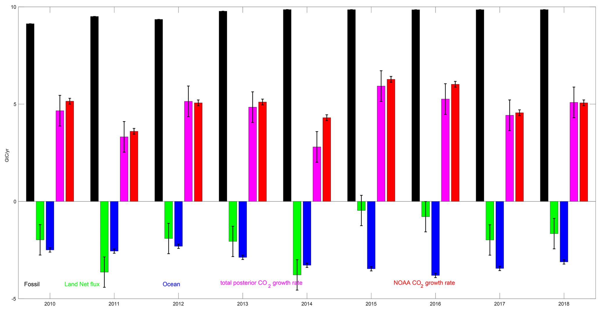
Figure 4 Global flux estimation and uncertainties from 2010–2018 (black: fossil fuel; green: posterior land fluxes; blue: ocean fluxes; magenta: estimated CO₂ growth rate; red: the NOAA CO₂ growth rate).

4 Characteristics of the dataset

4.1 Global fluxes

The annual atmospheric CO₂ growth rate, which is the net difference between fossil fuel emissions and total annual sink over land and ocean, is well observed by the NOAA surface CO₂ observing network (https://www.esrl.noaa.gov/gmd/ccgg/ggrn.php, last access: 12 March 2020). We compare the global total flux estimates constrained by GOSAT and OCO-2 with the NOAA CO₂ growth rate from 2010–2018 and discuss the mean carbon sink over land and ocean. Over these 9 years, the satellite-constrained atmospheric CO₂ growth rate agrees with the NOAA observed CO₂ growth rate within the uncertainty of the posterior fluxes (Fig. 4). The mean annual global surface CO₂ fluxes (in Gt C/yr) are derived from the NOAA observed CO₂ growth rate (in ppm/yr) using a conversion factor of 2.124 Gt C/ppm (Le Quéré et al., 2018). The estimated growth rate has the largest discrepancy with the NOAA observed growth rate in 2014, which may be due to a failure of one of the two solar paddles of GOSAT in May 2014 (Kuze et al., 2016). Over the 9 years, the estimated total accumulated carbon in the atmosphere is 41.5±2.4 Gt C, which is slightly lower than the accumulated carbon based on the NOAA CO₂ growth rate (45.2±0.4 Gt C). On average, we estimate that the NBE is 2.0±0.7 Gt C, $\sim \mathrm{20}\pm \mathrm{8}$ % of fossil fuel emissions, and the ocean sink is 3.0±0.1 Gt C, $\sim \mathrm{30}\pm \mathrm{1}$ % of fossil fuel emissions (Fig. 4). These numbers are within the ranges of the corresponding GCB estimates from Freidlingstein et al. (2019) (referred to as GCB-2019 hereafter). The mean NBE and ocean sink from GCB-2019 are 2.0±1.0 Gt C and 2.5±0.5 Gt C, respectively, which are 21±10 % and 26±5 % of fossil fuel emissions, respectively, between 2010–2018. The GCB does not report NBE directly, we calculate NBE from GCB-2019 as the residual differences between fossil fuel emissions, ocean net carbon sink, and atmospheric CO₂ growth rate. It is also equivalent to ($S_{\mathrm{LAND}}+B_{\mathrm{IM}}-E_{\mathrm{LUC}}$) reported by Freidlingstein et al. (2019), where S_LAND is terrestrial sink, B_IM is a budget imbalance, and E_LUC is land use change. Over these 9 years, we estimate that NBE ranges from 3.6 Gt C (∼37 % of fossil fuel emissions) in 2011 (a La Niña year) to only 0.5 Gt C (∼5 % of fossil fuel emissions) in 2015 (an El Niño year), consistent with 3.3 Gt C (35 % of fossil fuel) in 2011 to 0.9 Gt C (7 % of fossil fuel) in 2015 estimated from GCB-2019. We estimate that the ocean sinks range from 3.5 Gt C in 2015 to 2.3 Gt C in 2012, which is larger than the estimated ocean flux ranges of 2.7 in 2016 to 2.5 in 2012 reported by Freidlingstein et al. (2019).

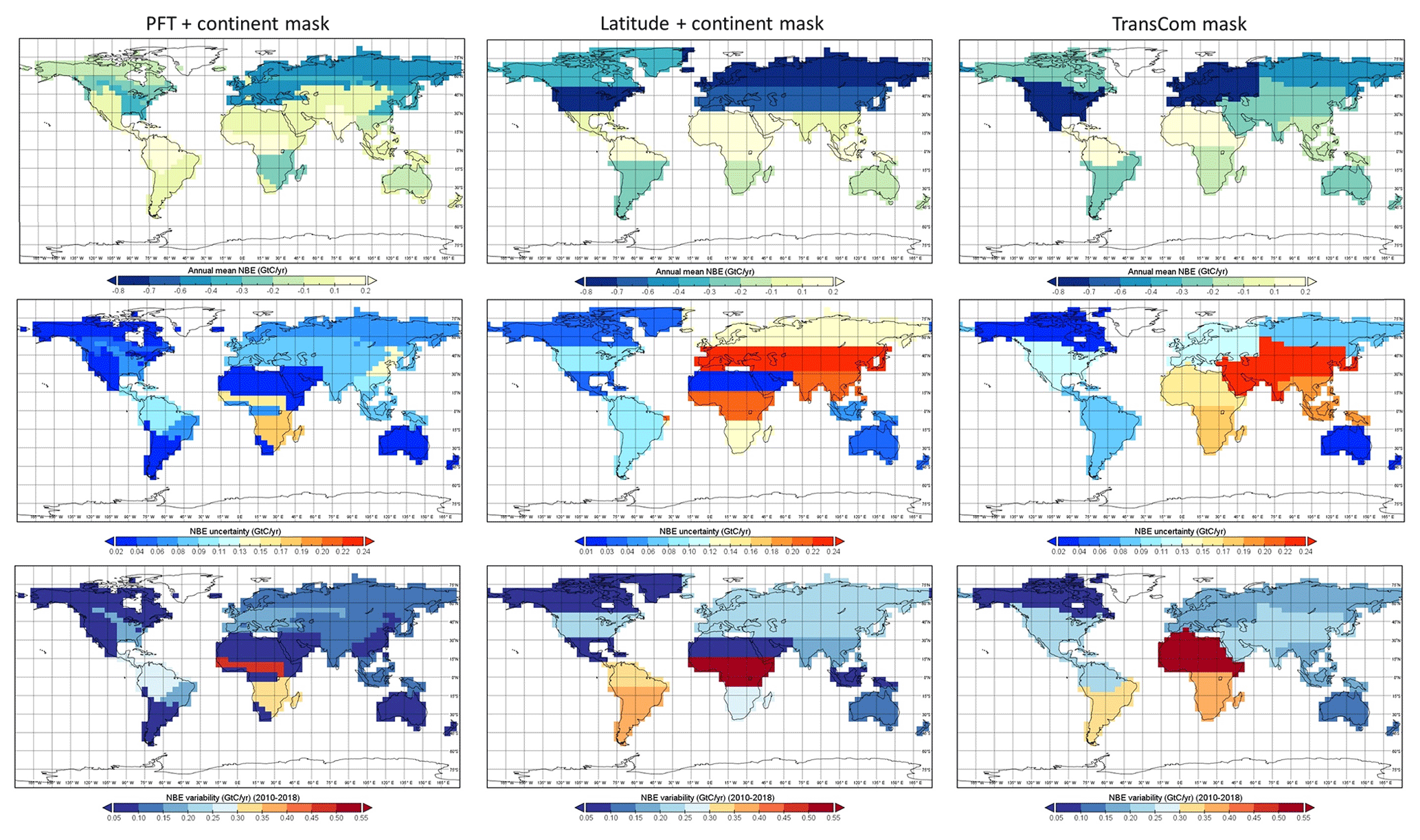
Figure 5 Mean annual regional NBE (a, b, c), uncertainty (d, e, f), and variability between 2010–2018 (g, h, i) with the three types of regional masks (Fig. 3). The first column uses a region mask based on plant functional types (PFTs) and continents (RM1). The second column uses a region mask based on latitude and continents (RM2), and the third column uses a TransCom mask.

4.2 Mean regional fluxes and uncertainties

Figure 5 shows the 9-year mean regional annual fluxes, uncertainty, and its variability between 2010–2018. Table 6 shows an example of the dataset corresponding to Fig. 5a, d, and g. It shows that large net carbon uptake occurs over Eurasia, NA, and the Southern Hemisphere (SH) midlatitudes. The largest net carbon uptake is over the eastern US ($-\mathrm{0.4}\pm \mathrm{0.1}$ Gt C (1σ uncertainty)) and high-latitude Eurasia ($-\mathrm{0.5}\pm \mathrm{0.1}$ Gt C) (Fig. 5a, b). We estimate a net land carbon sink of 2.5±0.3 Gt C/yr between 2010–2013 over the NH mid- to high latitudes, which agrees with 2.4±0.6 Gt C estimates over the same time periods based on a two-box model (Ciais et al., 2019). Net uptake in the tropics ranges from close to neutral in tropical South America (0.1±0.1 Gt C) to a net source in northern Africa (0.6±0.2 Gt C) (Fig. 5a, b). The tropics exhibit both large uncertainty and large variability. The NBE interannual variabilities over northern Africa and tropical SA are 0.5 and 0.3 Gt C, respectively, which are larger than the 0.2 and 0.1 Gt C uncertainty (Fig. 5d, e). We also find collocation of regions with large NBE and FLUXSAT GPP interannual variability (Fig. B4). The availability of flux estimates over the broadly used TransCom regions makes it easy to compare to previous studies. For example, we estimate that the annual net carbon uptake over North America is 0.7±0.1 Gt C/yr with 0.2 Gt C variability between 2010 and 2018, which agrees with 0.7±0.5 Gt C/yr estimates based on surface CO₂ observations between 1996–2007 (Peylin et al., 2013).

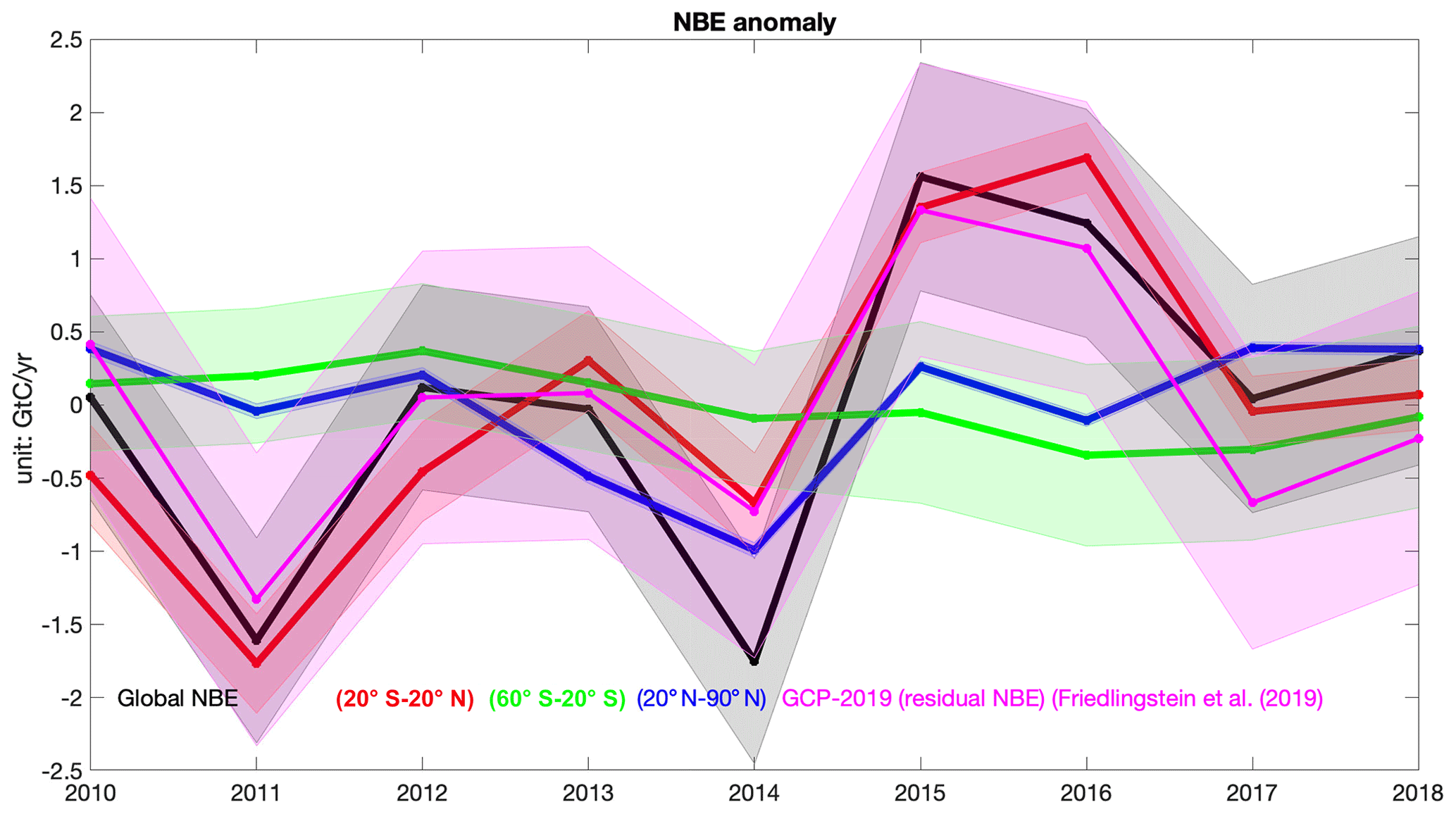
Figure 6 The NBE interannual variability over the globe (black), the tropics (20^∘ S–20^∘ N), SH midlatitudes (60–20^∘ S), and NH midlatitudes (20–90^∘ N). For reference, the residual net land carbon sink from GCB-2019 (Friedlingstein et al., 2019) and its uncertainty is also shown (magenta).

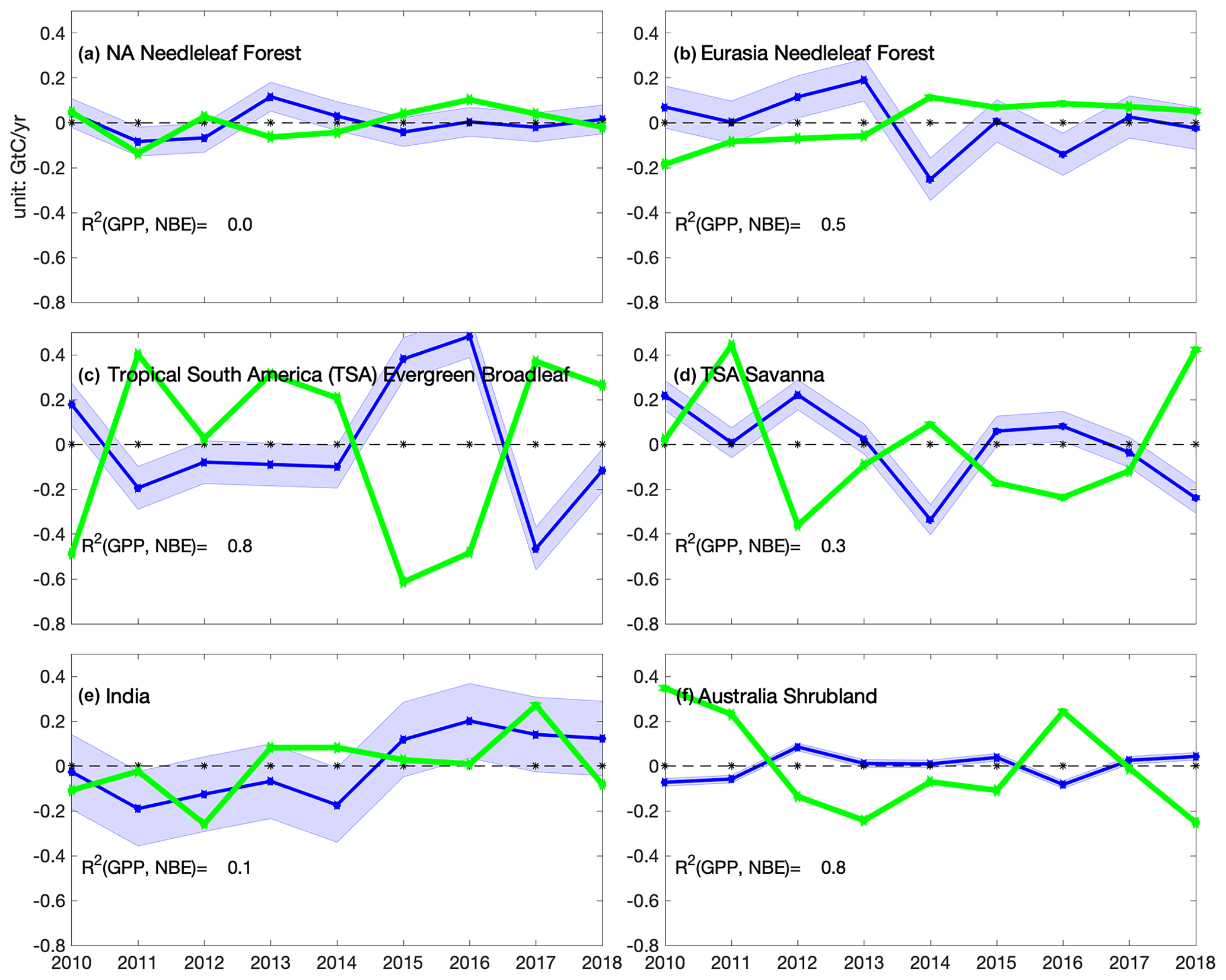
Figure 7 The NBE interannual variability over six selected regions. Blue: annual NBE anomaly and its uncertainties. Green: annual GPP anomaly based on FLUXSAT.

4.3 Interannual variabilities and uncertainties

Here we present hemispheric and regional NBE interannual variabilities and corresponding uncertainties (Figs. 6 and 7, and corresponding tabular data files). In Fig. 6, we further divide the globe into three large latitude bands: tropics (20^∘ S–20^∘ N), NH extra-tropics (20–85^∘ N), and SH extra-tropics (60–20^∘ S). The tropical NBE contributes 90 % to the global NBE interannual variability (IAV). The IAV of NBE over the extra-tropics is only about one-third of that over the tropics. The dominant role of tropical NBE in the global IAV of NBE agrees with Fig. 4 in Sellers et al. (2018). The top-down global annual NBE anomaly is within the 1.0 Gt C/yr uncertainty of residual NBE (i.e., fossil fuel–atmospheric growth–ocean sink) calculated from GCB-2019 (Friedlinston et al., 2019) (Fig. 6).

Figure 7 shows the annual NBE anomalies and uncertainties over a few selected regions based on RM1. Positive NBE indicates reduced net uptake relative to the 2010–2018 mean, and vice versa. Also shown in Fig. 7 are GPP anomalies estimated from FLUXSAT. Positive GPP indicates increased productivity, and vice versa. GPP drives NBE in years where anomalies are inversely correlated (e.g., positive NBE and negative GPP), and TER drives NBE in years where anomalies of GPP and NBE have the same sign or are weakly correlated. Over tropical SA evergreen broadleaf forest, the largest positive NBE anomalies occur during the 2015–2016 El Niño, corresponding to large reductions in productivity, consistent with Liu et al. (2017). In 2017, the region sees increased net uptake and increased productivity, implying a recovery from the 2015–2016 El Niño event. The variability in GPP explains 80 % of NBE variability over this region over the 9-year period. In Australian shrubland, our inversion captures the increased net uptake in 2010 and 2011 due to increased precipitation (Poulter et al., 2014) and increased productivity. The variability in GPP explains 70 % of the interannual variability in NBE. Over tropical South America savanna, the NBE interannual variability also shows strong negative correlations with GPP, with GPP explaining 40 % of NBE interannual variability. Over the midlatitude regions where the IAV is small, the R² between GPP and NBE is also small (0.0–0.5) as expected. But the increased net uptake generally corresponds to increased productivity. We also do not expect perfect negative correlation between NBE anomalies and GPP anomalies, as discussed in Sect. 2.5. The comparison between NBE and GPP provides insight into when and where net fluxes are likely dominated by productivity.

Table 5 List of the data products.

n/a: not applicable.

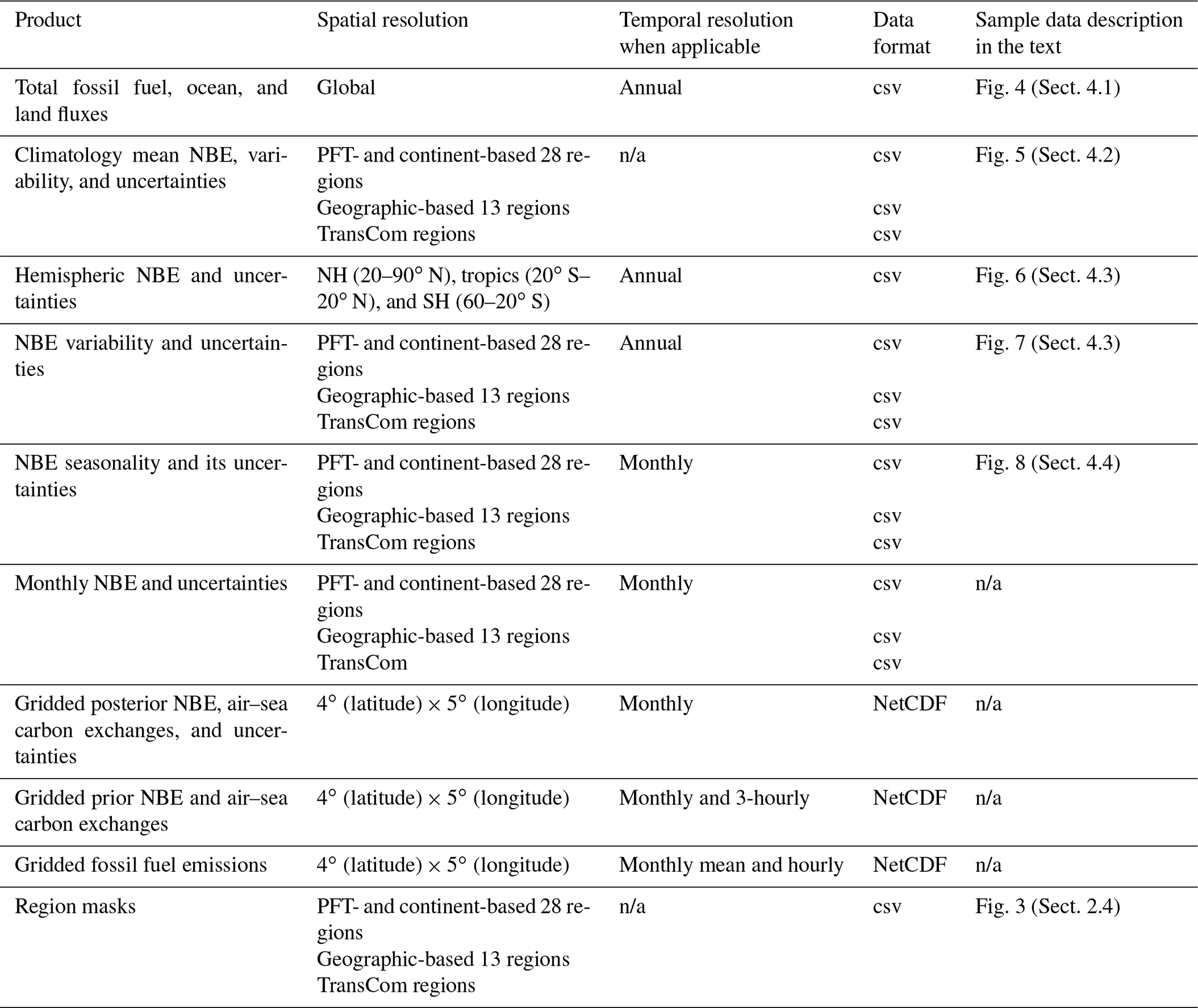
Table 6 The 9-year mean regional annual fluxes, uncertainties, and variability. Regions are based on the mask shown in Fig. 5a (Figure5.csv). Unit: Gt C/yr.

4.4 Seasonal cycle

We provide the regional mean NBE seasonal cycle, its variability, and uncertainty based on the three regional masks (Table 5). Here we briefly describe the characteristics of the NBE seasonal cycle over the 11 TransCom regions and its comparison to three independent top-down inversion results based on surface CO₂, which are CT-Europe (e.g., van der Laan-Luijkx et al., 2017), CAMS (Chevallier et al., 2005), and Jena CarbonScope (Rödenbeck et al., 2003). CMS-Flux NBE differs the most from surface-CO₂-based inversions over the South American tropical, northern Africa, tropical Asia, and NH boreal regions. The CMS-Flux NBE has a larger seasonal cycle amplitude over tropical Asia and northern Africa, where the surface CO₂ constraint is weak, while it has a smaller seasonal cycle amplitude over the boreal region; this may be due to the sparse satellite observations over the high latitudes and weaker seasonal amplitude of the prior CARDAMOM fluxes. The comparison to FLUXSAT GPP can only qualitatively evaluate the NBE seasonal cycle but cannot differentiate among different estimates. In general, the months that have larger productivity correspond to months with a net uptake of carbon from the atmosphere, especially over the NH (Fig. 8). More research is still needed to understand the seasonal cycles of NBE, including its phase (i.e., transition from source to sink) and amplitude (peak-to-trough difference), as well as its relationships with GPP and respiration.

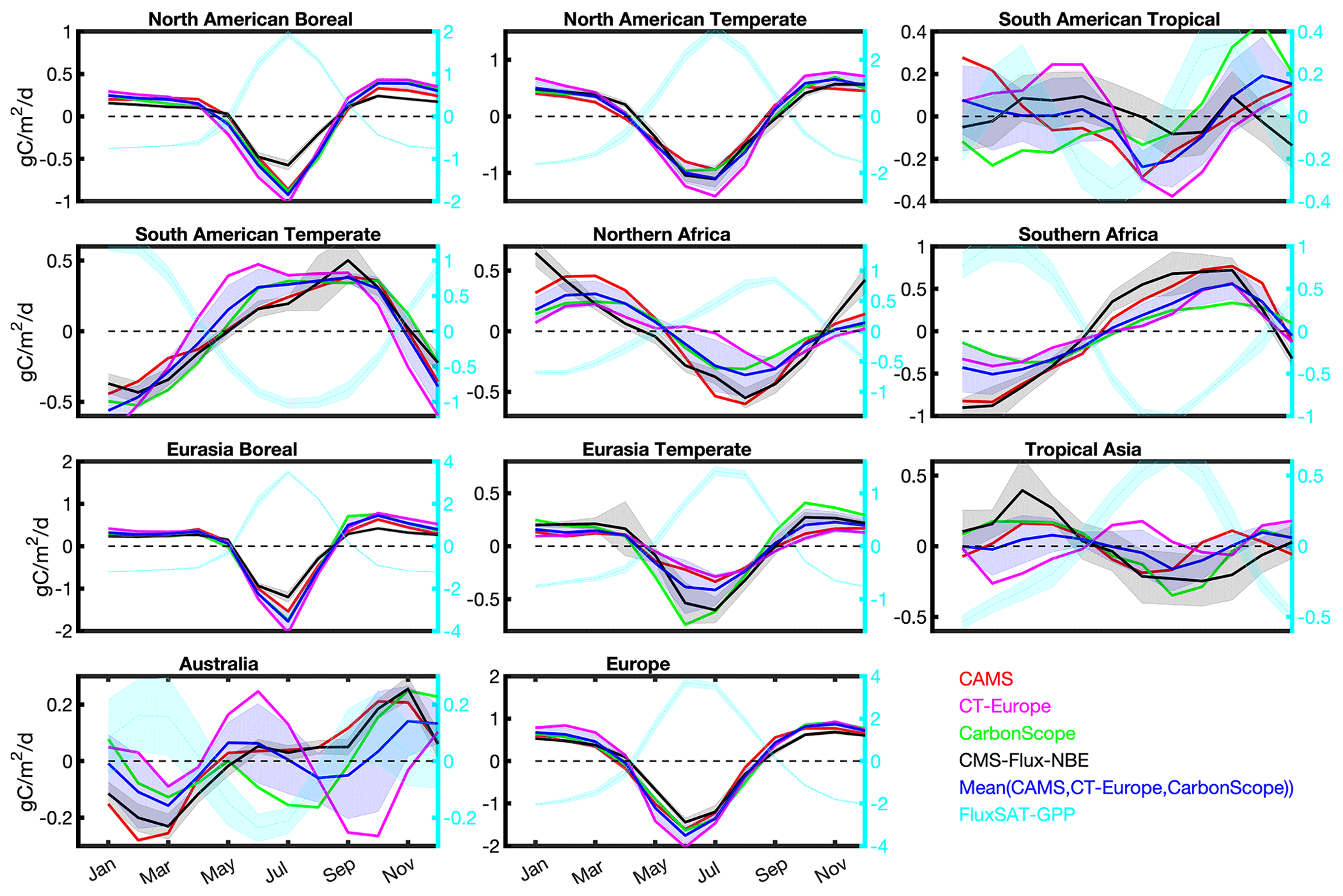
Figure 8 The NBE climatological seasonality over TransCom regions. The seasonal cycle is calculated over 2010–2017 since CT-Europe only covers until 2017. Black: CMS-Flux NBE and its uncertainty; blue shaded: mean NBE seasonality based on surface CO₂ inversion results from CAMS, CT-Europe, and Jena CarbonScope; red: CAMS; magenta: CT-Europe; green: Jena CarbonScope. The names of each region are shown on individual subplots.

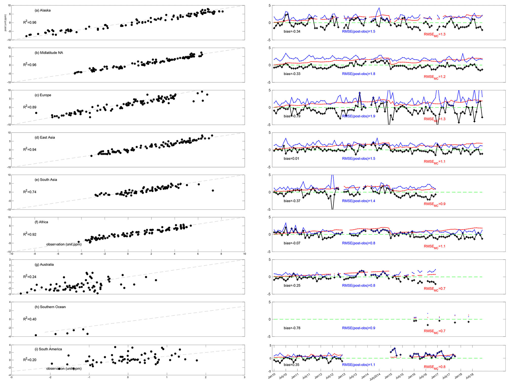
Figure 9 Comparison between posterior CO₂ mole fraction and aircraft observations. Left panel: detrended posterior CO₂ (y axis) vs. detrended aircraft CO₂ (x axis) over nine regions. The dashed line is the one-to-one line; right panel: the differences between posterior CO₂ and aircraft CO₂ as a function of time (black), RMSE (blue; unit: ppm), and RMSE_MC (red).

5 Evaluation against independent aircraft CO₂ observations

5.1 Comparison to aircraft observations over nine sub-regions

In this section, we evaluate posterior CO₂ against aircraft observations over the nine sub-regions listed in Table 4 and Fig. 2. We compare the posterior CO₂ to aircraft CO₂ mole fractions above the planetary boundary layer and up to the mid-troposphere (1–5 km) at the locations and time of aircraft observations, and then we calculate the monthly mean error statistics between 1–5 km. The aircraft observations between 1–5 km are more sensitive to regional fluxes (Liu et al., 2015; Liu and Bowman, 2016). Scatter plots in the left column of Fig. 9 show regional monthly mean detrended aircraft CO₂ observations (x axis) versus the simulated detrended posterior CO₂ (y axis). We used the NOAA global CO₂ trend to detrend both the observations and model-simulated mole fractions (ftp://aftp.cmdl.noaa.gov/products/trends/co2/co2_trend_gl.txt, last access: 19 May 2020). Over the NH regions (Fig. 9a, b, c, d) and Africa (Fig. 9f), the R² is greater than or equal to 0.9, which indicates that the posterior CO₂ captures the observed seasonality. The low R² (0.7) value in South Asia is caused by one outlier. Over the Southern Ocean, Australia, and SA, the R² is between 0.2 and 0.4, reflecting weaker CO₂ seasonality over these regions and possible bias in ocean flux estimates (see discussions later).

The right panel of Fig. 9 shows the monthly mean differences between posterior CO₂ and aircraft observations (black), RMSE (Eq. 2) (blue line), and RMSE_MC (Eq. 3) (red line). The magnitude of the mean differences between the posterior CO₂ and aircraft observations is less than 0.5 ppm, except over the Southern Ocean, which has a −0.8 ppm bias. The mean differences between posterior CO₂ and aircraft observations are primarily caused by errors in transport and biases in assimilated satellite observations, while RMSE_MC is the internal flux error projected into mole fraction space. With the exception of the Southern Ocean, for all regions mean bias is significantly less than RMSE_MC, which suggests that transport and data bias in satellite observations may be much smaller than the internal flux errors. Note that RMSE_MC is smaller than RMSE over the first ∼ 6 months of simulation, which may indicate a dominant impact of errors in transport and initial CO₂ concentration on posterior CO₂ RMSE.

As demonstrated in Sect. 2.5, comparing RMSE and RMSE_MC is a test of the accuracy of posterior flux uncertainty estimate. Over all the regions, the differences between RMSE and RMSE_MC are smaller than 0.3 ppm, which indicates a comparable magnitude between empirical posterior flux uncertainty estimates from the Monte Carlo method and the actual posterior flux uncertainty over the regions that these aircraft observations are sensitive to. These aircraft observations are sensitive to NBE over a broad region as shown in Fig. B5. Note that Figs. B5 and B8–B10 are calculated using Eq. (8).

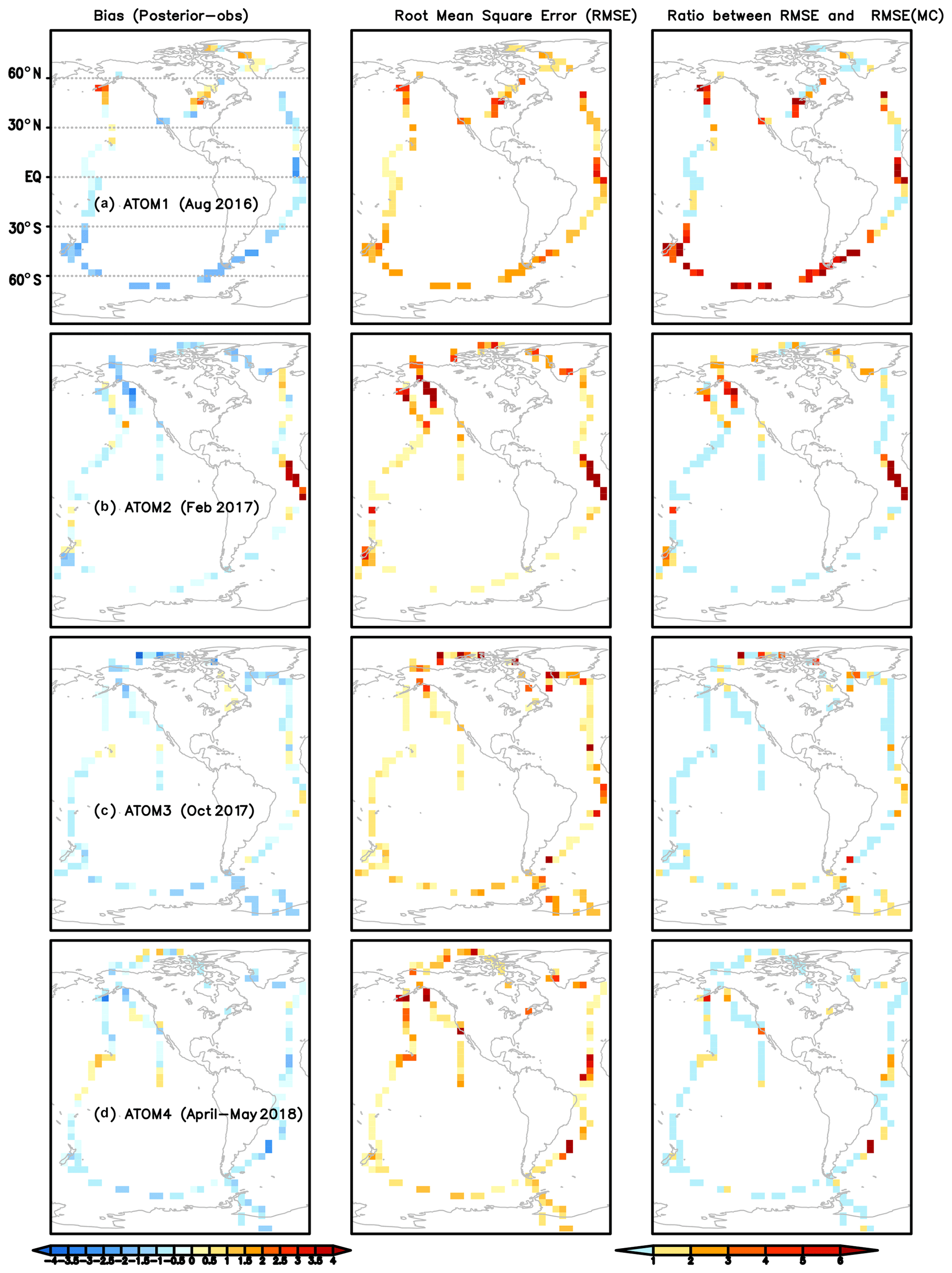
Figure 10 Left column: the mean differences between posterior CO₂ and aircraft observations from ATom 1–4 aircraft campaigns between 1–5 km (a–d). Middle column: the root mean square errors (RMSEs) between aircraft observations and posterior CO₂ between 1–5 km. The color bar is the same as in the left column. Right column: the ratio between RMSE and RMSE_MC based on ensemble CO₂ from the Monte Carlo uncertainty estimation method.

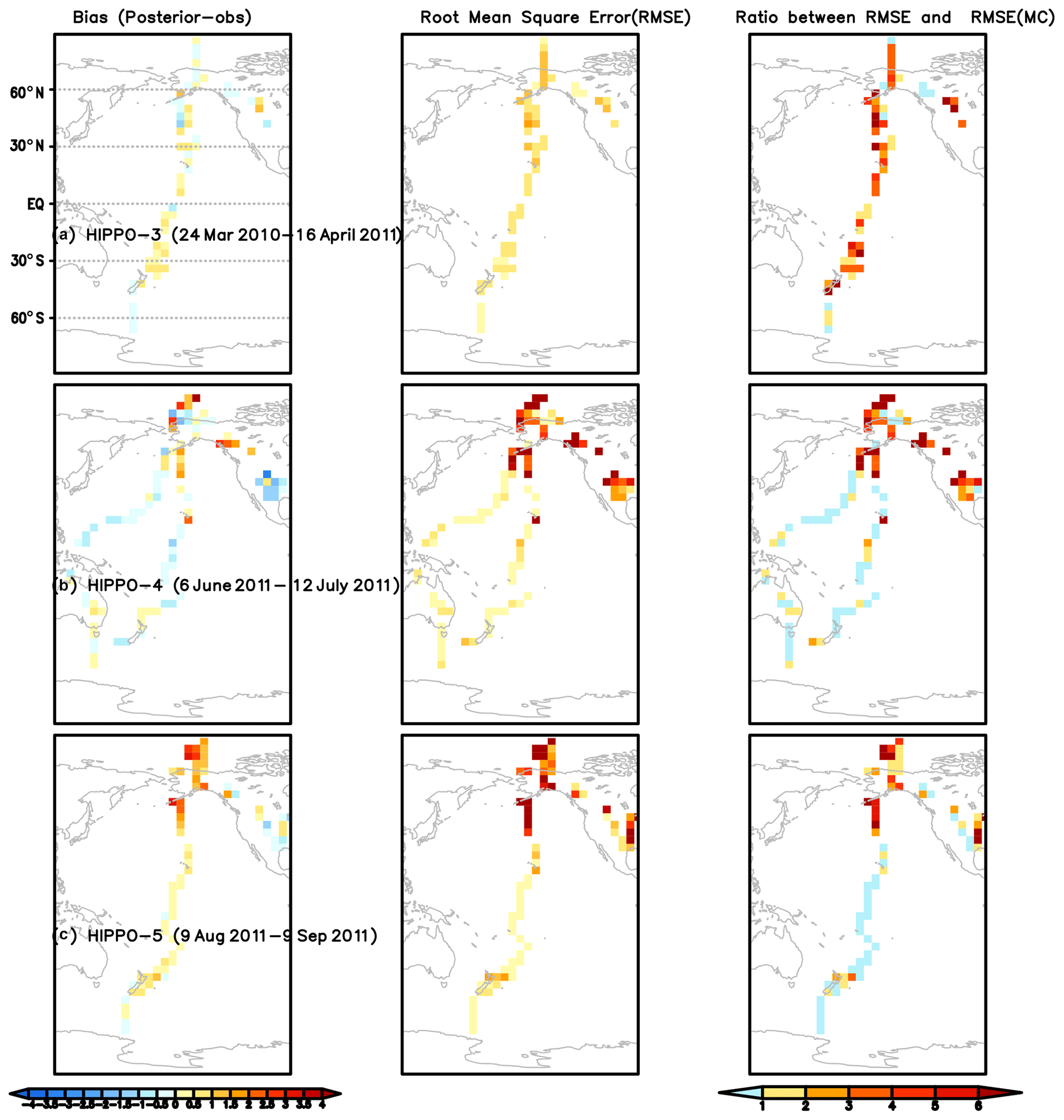
Figure 11 Left column: the mean differences between posterior CO₂ and aircraft observations from HIPPO 3–5 aircraft campaigns between 1–5 km (a–c) (unit: ppm). The time frame of each campaign is in the figure. Middle column: the root mean square errors (RMSEs) between aircraft observations and posterior CO₂ between 1–5 km (unit: ppm). The color bar is the same as in the left column. Right column: the ratio between RMSE and RMSE_MC based on ensemble CO₂ from the Monte Carlo method.

5.2 Comparison to aircraft observations from ATom and HIPPO aircraft campaigns

Figures 10 and 11 show comparisons to aircraft CO₂ from the ATom 1–4 campaigns spanning four seasons and HIPPO 3–5 over the Pacific Ocean between 1–5 km. The vertical curtain comparisons are shown in Figs. B6 and B7. The mean differences between posterior CO₂ and aircraft CO₂ are quite uniform (within 0.5 ppm) throughout the column, except over the Atlantic Ocean during ATom 1–2 and the Southern Ocean during ATom 1 (Figs. S6 and S7). Also shown in Figs. 10 and 11 are RMSEs of each aircraft campaign (middle column) and the ratio between RMSE and RMSE_MC (right column). A ratio larger than one between RMSE and RMSE_MC indicates errors in either transport or underestimation of the posterior flux uncertainty (Sect. 2.5).

Over most of the flight tracks during ATom 1–4, the posterior CO₂ errors are between −0.5 and 0.5 ppm, the RMSE is smaller than 0.5 ppm, and the ratio between RMSE and RMSE_MC is smaller than or equal to 1. However, off the coast of Africa during ATom 1 and 2 and over the Southern Ocean during ATom 1, the mean differences between posterior CO₂ and aircraft observations are larger than 0.5 ppm. During ATom 1 (29 July–23 August 2016), the mean differences between posterior CO₂ and aircraft CO₂ show large negative biases, while during ATom 2 (26 January–21 February 2017) it has large positive biases off the coast of Africa. The ratio between RMSE and RMSE_MC is significantly larger than one over these regions, which indicates an underestimation of posterior flux uncertainty or a large magnitude of transport errors during that time period.

We further run adjoint sensitivity analyses over the three regions with ratios significantly larger than one to identify the posterior fluxes that could contribute to the large differences between posterior CO₂ and aircraft observations during ATom 1–2. We run the adjoint model backward for 3 months from the observation time and calculate S_i as defined in Eq. (7). The adjoint sensitivity analysis indicates that the large mismatch between aircraft observations and model simulations during ATom 1 and -2 off the coast of Africa could be potentially driven by errors in posterior fluxes over tropical Africa (Fig. B8). The large posterior CO₂ errors and large ratio between RMSE and RMSE_MC over the Southern Ocean during ATom 1 are driven by flux errors in oceanic fluxes around 30^∘ S and over Australia (Fig. B9), which also contribute to the large errors in comparison to aircraft observations over the Southern Ocean shown in Fig. 9h.

During the HIPPO aircraft campaigns, the absolute errors in posterior CO₂ across the Pacific are less than 0.5 ppm, except over the Arctic Ocean and over Alaska in summer (Fig. 11), consistent with Fig. 10a. The large errors over the Arctic Ocean may be related to both transport errors and the accuracy of high-latitude fluxes. Byrne et al. (2020) provide a brief summary of the challenges in simulating CO₂ over high latitudes using a transport model with 4^∘ × 5^∘ resolution. Increasing the resolution of the transport model may reduce transport errors over high latitudes.

We run adjoint sensitivity analyses over the high-latitude regions where the differences between posterior CO₂ and aircraft observations are large (Fig. 11). The adjoint sensitivity analysis (Fig. B10) shows that the large errors over these regions could be driven by errors in fluxes over Alaska as well as broad NH midlatitude regions.

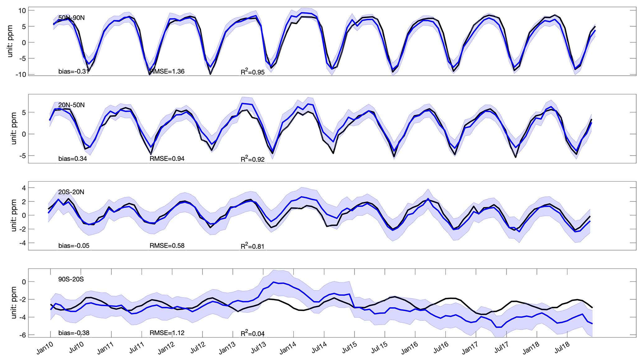
Figure 12 Comparison between posterior CO₂ and the NOAA marine boundary layer (MBL) reference sites. Black: observations averaged over each latitude band; blue and shaded area: posterior CO₂ and its uncertainty. The global mean CO₂ (https://www.esrl.noaa.gov/gmd/ccgg/trends/global.html, last access: 29 May 2020) was subtracted from both the NOAA MBL reference and posterior CO₂ before the comparison.

5.3 Comparison to MBL reference sites

Since MBL reference sites sample air over broad regions, the comparison to detrended MBL observations indirectly evaluates the NBE over large regions. Figure 12 shows the comparison over four latitude bands. The uncertainty of posterior CO₂ concentration is from the MC method. Except over 90–20^∘ S, the differences between observations and posterior CO₂ are within posterior CO₂ uncertainty estimates. The posterior CO₂ concentrations have the smallest bias and random errors over the tropical latitude band. The R² is above 0.9 over NH mid- to high latitudes, consistent with Fig. 9. Over 90–20^∘ S, the posterior CO₂ has positive bias in 2013 and 2014 and negative bias and much weaker seasonality between January 2015–December 2018 compared to observations, which indicates possible biases in Southern Ocean flux estimates (Fig. B11). The low bias over the Southern Ocean is consistent with aircraft comparison during the OCO-2 period (Figs. 9–10, B9). The changes of performance after 2013 over 90–20^∘ S are most likely due to the prior ocean carbon fluxes. Evaluation of ocean carbon fluxes is out of the scope of this study. Note that since we only assimilate land nadir X${}_{{\mathrm{CO}}_{\mathrm{2}}}$ observations in this study due to known issues with the OCO-2 v9 ocean glint observations (O'Dell et all., 2018), the constraint of top-down inversion on air–sea CO₂ exchanges is weak (not shown). The ocean glint observations of OCO-2 v10 observations have been improved compared to v9 (Osterman et al., 2020). We expect to have a better estimate of ocean carbon fluxes over the Southern Ocean when assimilating both land and ocean X${}_{{\mathrm{CO}}_{\mathrm{2}}}$ observations from GOSAT and OCO-2 in the future.

6 Discussion

Evaluation of posterior flux uncertainty estimates by comparing posterior CO₂ error statistics (RMSE, Eq. 2) with the standard deviation of ensemble simulated CO₂ from the Monte Carlo uncertainty quantification method (RMSE_MC, Eq. 3) has its limitations. A comparable RMSE and RMSE_MC indicates a small magnitude of transport errors and reasonable posterior uncertainty estimates. A much larger RMSE than RMSE_MC could be due to errors in either transport or underestimation of the posterior flux uncertainty or both. The presence of transport errors makes the interpretation of the RMSE and RMSE_MC complex. A better, independent quantification of transport errors is needed in the future in order to rigorously use the comparison statistics between aircraft observations and posterior CO₂ to diagnose flux errors.

Comparison to aircraft observations shows regionally dependent accuracy in posterior fluxes. ATom observations show seasonally dependent biases over the Atlantic, implying possible seasonally dependent errors in posterior fluxes over northern to central Africa. Therefore, we recommend combining NBE with other ancillary variables, e.g., GPP, to better understand carbon dynamics. Combining NBE with component carbon fluxes can shed light on the processes controlling the changes of NBE (e.g., Bowman et al., 2017; Liu et al., 2017). NBE can be written as

$$\begin{array}{}\text{(9)}& \text{NBE}=\text{TER}+\text{fire}-\text{GPP},\end{array}$$

where TER is total ecosystem respiration (TER) (Fig. 1). Satellite carbon monoxide (CO) observations provide constraints on fire emissions (Arellano et al., 2006; van der Werf, 2008; Jones et al., 2009; Jiang et al., 2017; Bowman et al., 2017; Liu et al., 2017). In addition to the FLUXSAT GPP product used here, solar-induced chlorophyll fluorescence (SIF) can be directly used as a proxy for GPP (e.g., Parazoo et al., 2014). Once NBE, fire, and GPP carbon fluxes are quantified, TER can be calculated as a residual (e.g., Bowman et al., 2017; Liu et al., 2017, 2018).

Because of the diffusive manner of atmospheric transport and the limited observation coverage, the gridded flux values are not independent from each other. The errors and uncertainties of the fluxes at each individual grid point are larger than regional aggregated fluxes. Interpreting NBE at each individual grid point requires caution. But at the same time, satellite CO₂-constrained NBE can potentially resolve fluxes at spatial scales smaller than the traditional TransCom regions. Here, we provide regional fluxes at two predefined regions in addition to TransCom. We encourage data users to use the data at appropriate regional scales.

The variability and changes are more robust than the mean NBE fluxes from top-down flux inversions in general (Baker et al., 2006b). The errors in transport and potential biases in observations are mostly stable in time, so biases in the mean fluxes tend to cancel out when computing interannual variability and year-to-year changes (Schuh et al., 2019; Crowell et al., 2019).

The global fossil fuel emissions have ∼5 % uncertainty (GCB-2019). However, they are regionally inhomogeneous. We neglect the uncertainties in fossil fuel emissions, which will introduce additional error in regions of rapid fossil fuel growth or in areas with noisier statistics (Yin et al., 2019). In the future, we will account for uncertainties in fossil fuel emissions.

The posterior NBE includes all types of land fluxes except fossil fuel emissions, which is equivalent to the sum of land use change fluxes, land sinks, and residual imbalance published by the GCB-2019. The sum of regional NBE and fossil fuel emissions is an index of the contribution of any specific region to the changes of the atmospheric CO₂ growth rate. Since the predicted changes of NBE in the future have large uncertainties (Lovenduski and Bonan, 2017), quantifying regional NBE is critical to monitoring regional contributions to atmospheric CO₂ growth rate and ultimately to guiding mitigation to limit warming to 1.5 ^∘C above pre-industrial levels (IPCC, 2021).

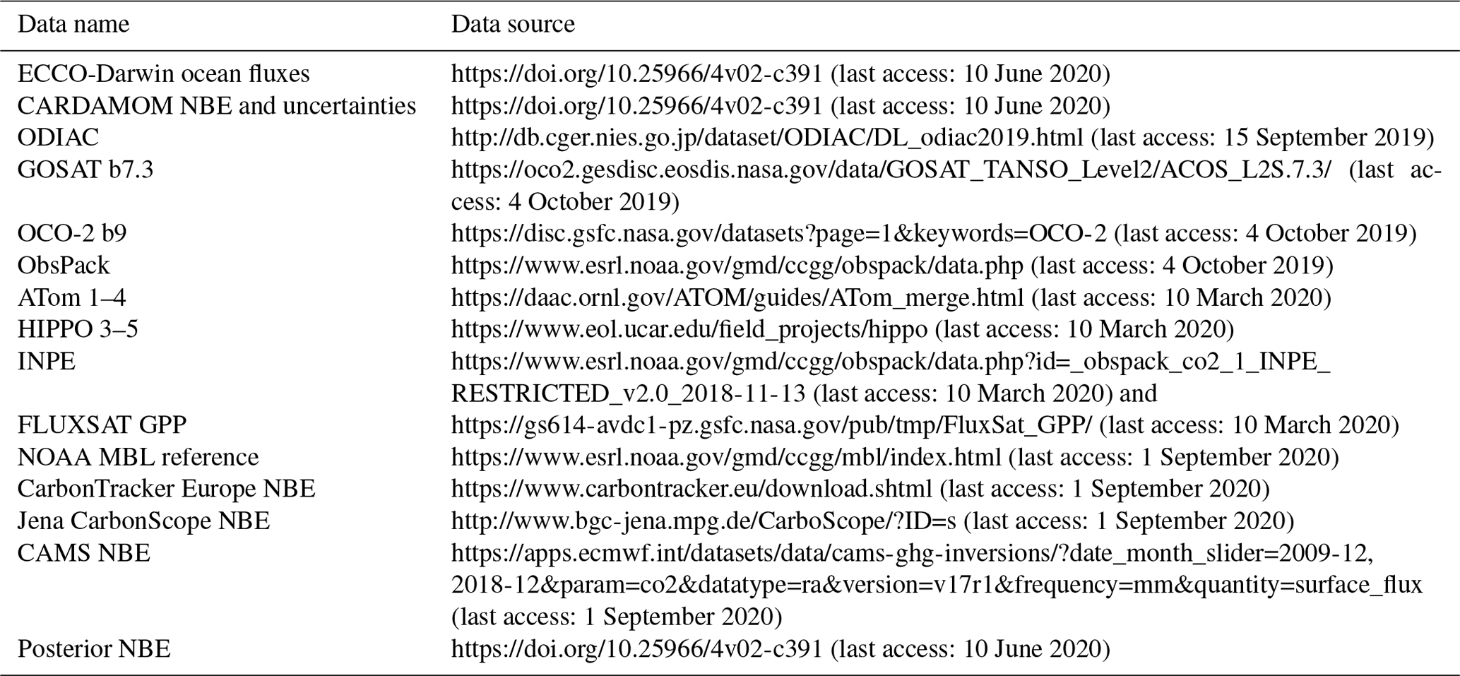
Table 7 Lists of data sources used in producing and evaluating the posterior NBE product.

7 Data availability

The CMS-Flux NBE 2020 data are available at https://doi.org/10.25966/4v02-c391 (Liu et al., 2020). The regional aggregated fluxes are provided as csv files with file size ∼10 MB, and the gridded data are provided in NetCDF format with file size ∼1.4 GB. The full ensemble of posterior fluxes used to estimate posterior flux uncertainties is provided in NetCDF format with file size ∼30 MB. Table 7 lists the sources of the data used in producing and evaluating the CMS-Flux NBE 2020 data product.

The quality of X${}_{{\mathrm{CO}}_{\mathrm{2}}}$ from satellite observations is continually improving. The OCO-2 v10 X${}_{{\mathrm{CO}}_{\mathrm{2}}}$ was released in June 2020 along with the full GOSAT record (June 2009–January 2020) processed by the same retrieval algorithm as OCO-2. Continuing to improve the quality of satellite observations and extending the NBE estimates beyond 2018 in the future will help us better understand interactions between the terrestrial biosphere carbon cycle and climate and provide support in monitoring the regional contributions to the changes of atmospheric CO₂. Thus, we plan a future update of the dataset on an annual basis, with a goal to support current scientific research and policy making.

8 Summary

Terrestrial biosphere carbon fluxes are the largest contributor to the interannual variability of the atmospheric CO₂ growth rate. Therefore, monitoring its change at regional scales is essential for understanding how it responds to CO₂, climate, and land use. Here, we present the longest terrestrial flux estimates and their uncertainties constrained by X${}_{{\mathrm{CO}}_{\mathrm{2}}}$ from 2010–2018 on self-consistent global and regional scales (CMS-Flux NBE 2020). We qualitatively evaluate the NBE estimates by comparing its variability with GPP variability and provide a comprehensive evaluation of posterior fluxes and the uncertainties by comparing posterior CO₂ with independent CO₂ observations from aircraft and the NOAA MBL reference sites. This dataset can be used in understanding controls on regional NBE interannual variability, evaluating biogeochemical models, and supporting the monitoring of regional contributions to changes in atmospheric CO₂.

Appendix A

As shown in Kalnay (2003),

$$\begin{array}{}\text{(A1)}& {\text{RMSE}}^{\mathrm{2}}={\displaystyle \frac{\mathrm{1}}{n}}\sum _{i=\mathrm{1}}^n({\mathbf{R}}_{i,i}+({\mathbf{HP}}^a{\mathbf{H}}^T{)}_{i,i}),\end{array}$$

where R_i,i is the ith aircraft observation error variance, and P^a is the posterior flux error covariance. The H is the linearized observation operator, which transfers posterior flux errors to aircraft observation space, and H^T is its adjoint. In the Monte Carlo method, the posterior flux error covariance P^a is approximated by

$$\begin{array}{}\text{(A2)}& {\mathbf{P}}^a={\displaystyle \frac{\mathrm{1}}{n\mathrm{ens}}}{\mathbf{X}}^a{\mathbf{X}}^{aT},\end{array}$$

where X^a is the ensemble perturbations written as

$$\begin{array}{}\text{(A3)}& {\mathbf{X}}^a={\mathbf{x}}^a-{\overline{\mathit{x}}}^a,\end{array}$$

where x^a is the ensemble posterior fluxes from the Monte Carlo simulations, and ${\overline{\mathit{x}}}^a$ is the mean.

Therefore, HP^aH^T can be written as

$$\begin{array}{}\text{(A4)}& {\mathbf{HP}}^a{\mathbf{H}}^T={\displaystyle \frac{\mathrm{1}}{n\mathrm{ens}}}\left[h\right({\mathbf{x}}^a)-h({\overline{\mathit{x}}}^a\left)\right]\left[h\right({\mathbf{x}}^a)-h({\overline{\mathit{x}}}^a){]}^T.\end{array}$$

The sum of diagonal elements in the right-hand side of Eq. (A4) is the same as the definition of RMSE_MC in the main text.

Therefore, when the posterior flux uncertainty estimated by the Monte Carlo method represents the actual uncertainty in posterior fluxes, Eq. (A1) can be written as

$$\begin{array}{}\text{(A5)}& {\text{RMSE}}^{\mathrm{2}}={\displaystyle \frac{\mathrm{1}}{n}}\sum _{i=\mathrm{1}}^n{\mathbf{R}}_{i,i}+{\text{RMSE}}_{\mathrm{MC}}^{\mathrm{2}}.\end{array}$$

It is the same as Eq. (4) in the main text.

Appendix B

In this Appendix, we include figures to support the main text.

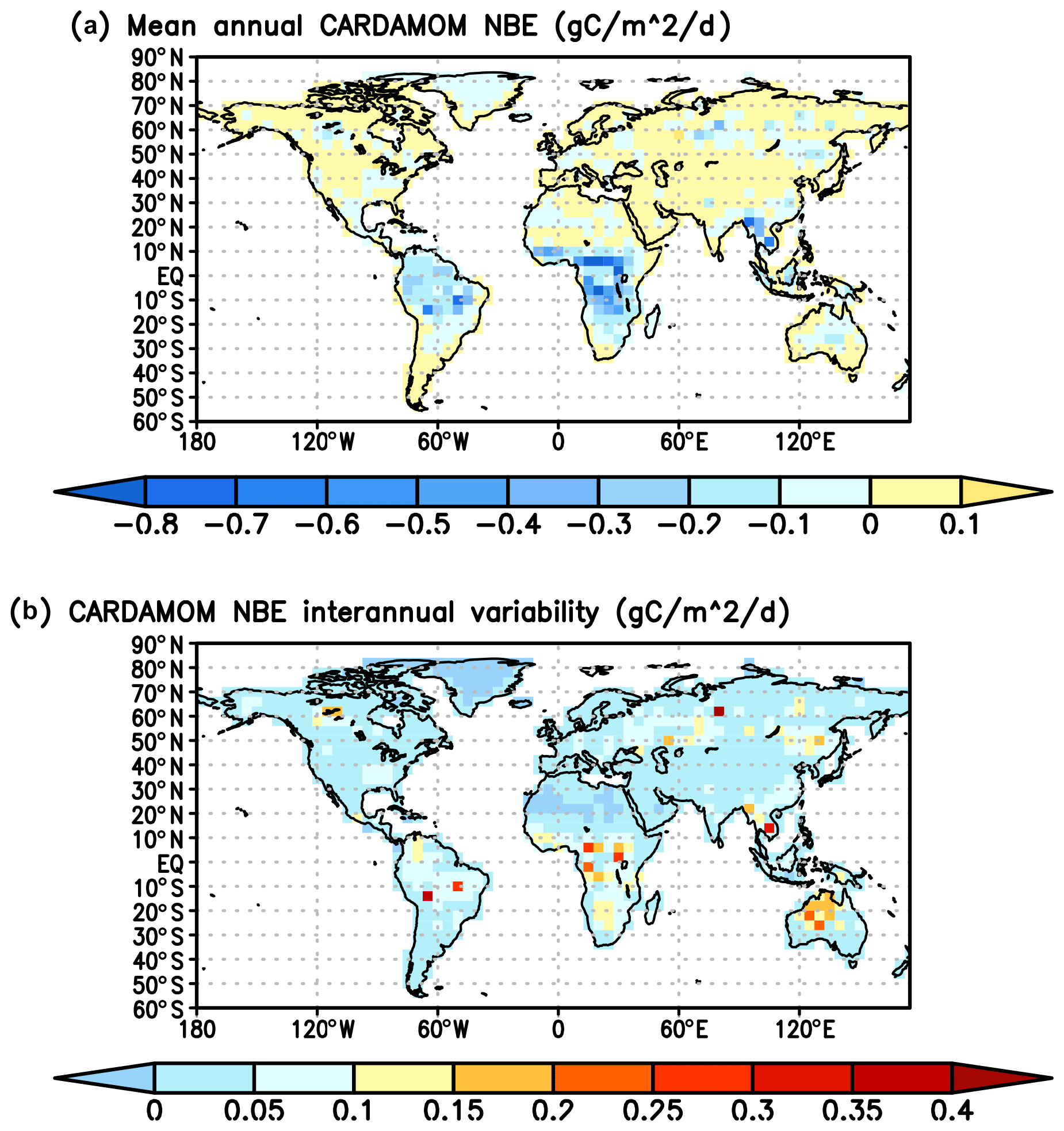
Figure B1 Annual mean net biosphere exchanges from CARDAMOM (a) and its interannual variability between 2010 and 2017 (b).

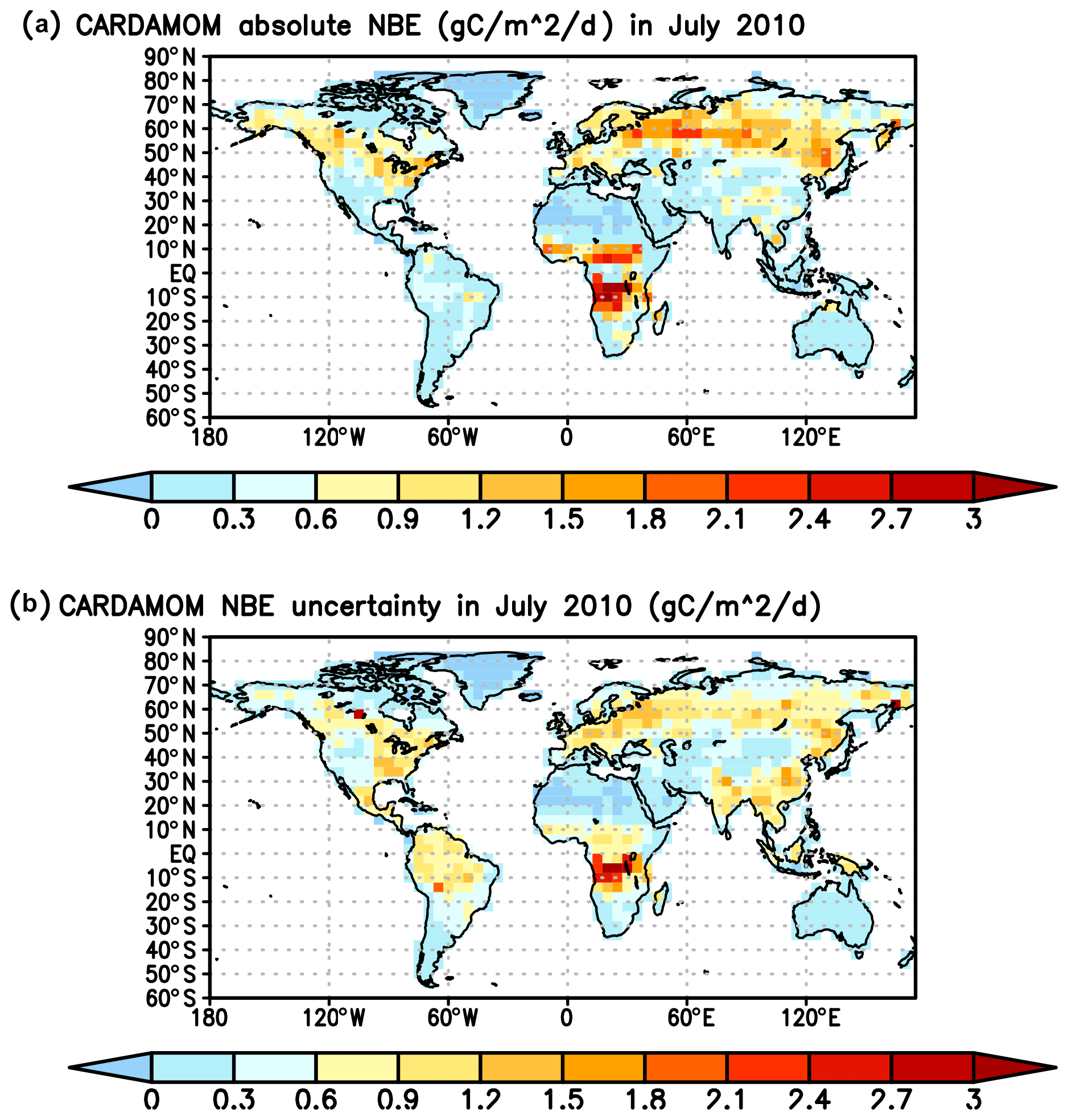
Figure B2 An example of absolute mean NBE (a) and its uncertainty (b) simulated by CARDAMOM. This is for July 2010.

Figure B3 Daily number of ACOS-GOSAT b7.3 (a) and OCO-2 super observations (b) assimilated in the top-down inversions.

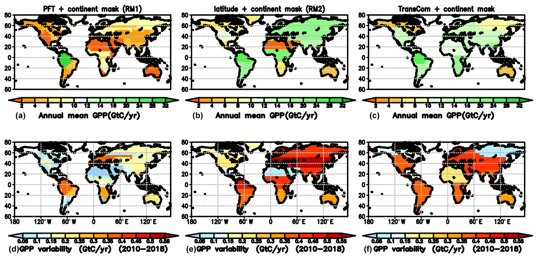
Figure B4 Regional mean FLUXSAT GPP and its variability between 2010–2018. (a, b, c) Regional mean GPP aggregated with the three regional masks; (d, e, f) GPP variability between 2010–2018. Unit: Gt C/yr.

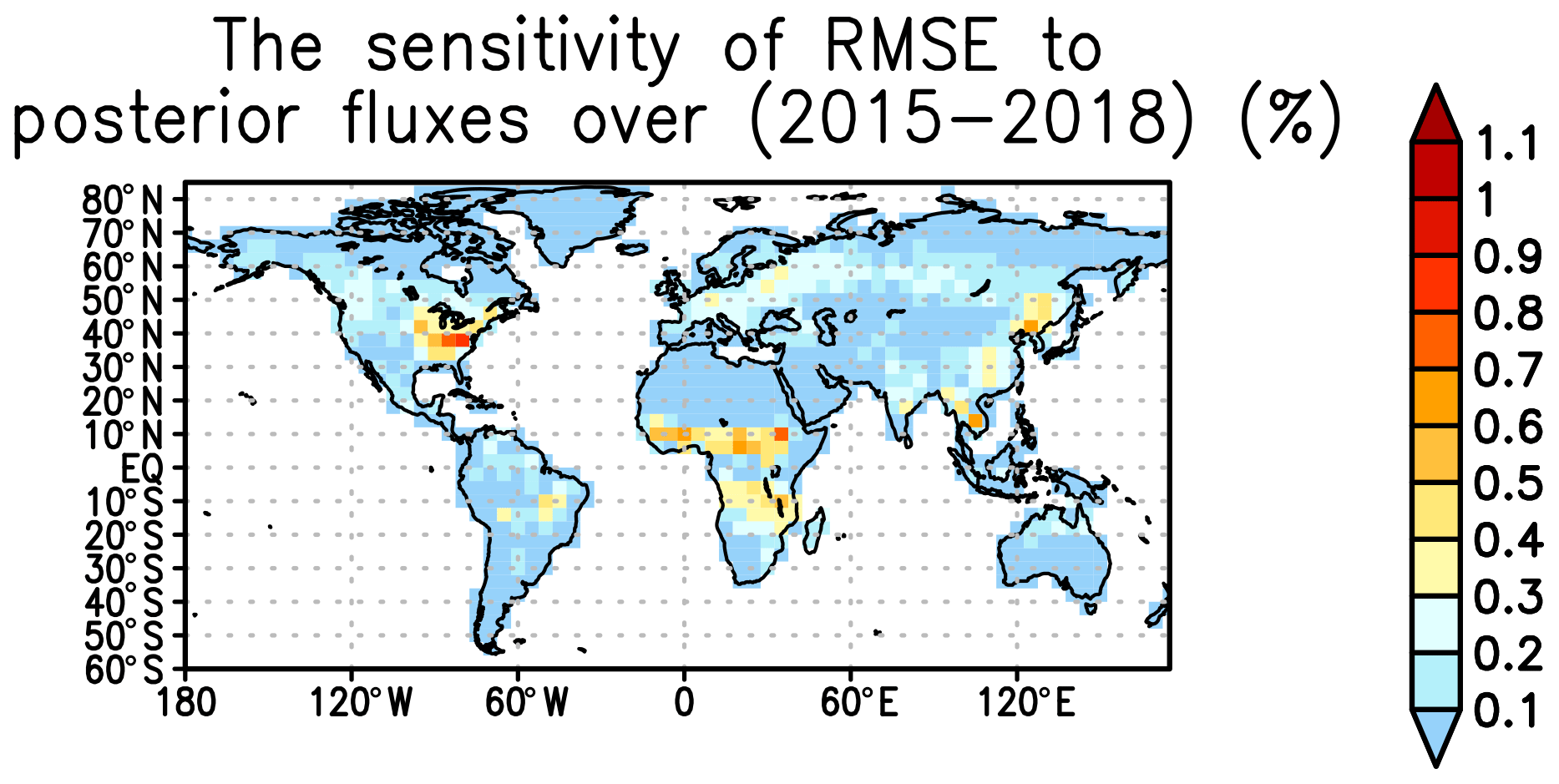
Figure B5 The relative sensitivity of root mean square errors (RMSEs) of posterior CO₂ (Fig. 9 in the main text) relative to NBE at every grid point. The adjoint model is carried out over September 2014–December 2018.

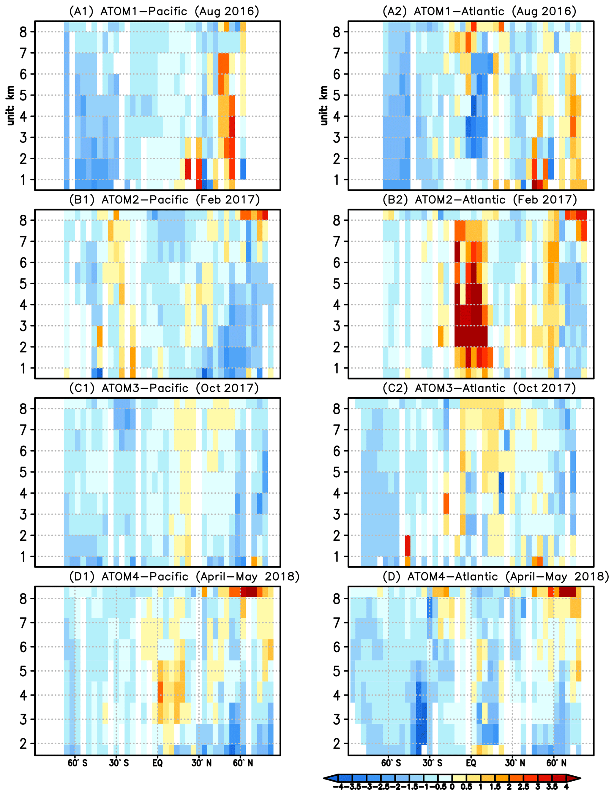
Figure B6 Differences between posterior CO₂ and ATom 1–4 aircraft CO₂ observations over the Pacific (A1–D1) and Atlantic Ocean (A2–D2) as a function of latitude and altitude (unit: km). Unit: ppm.

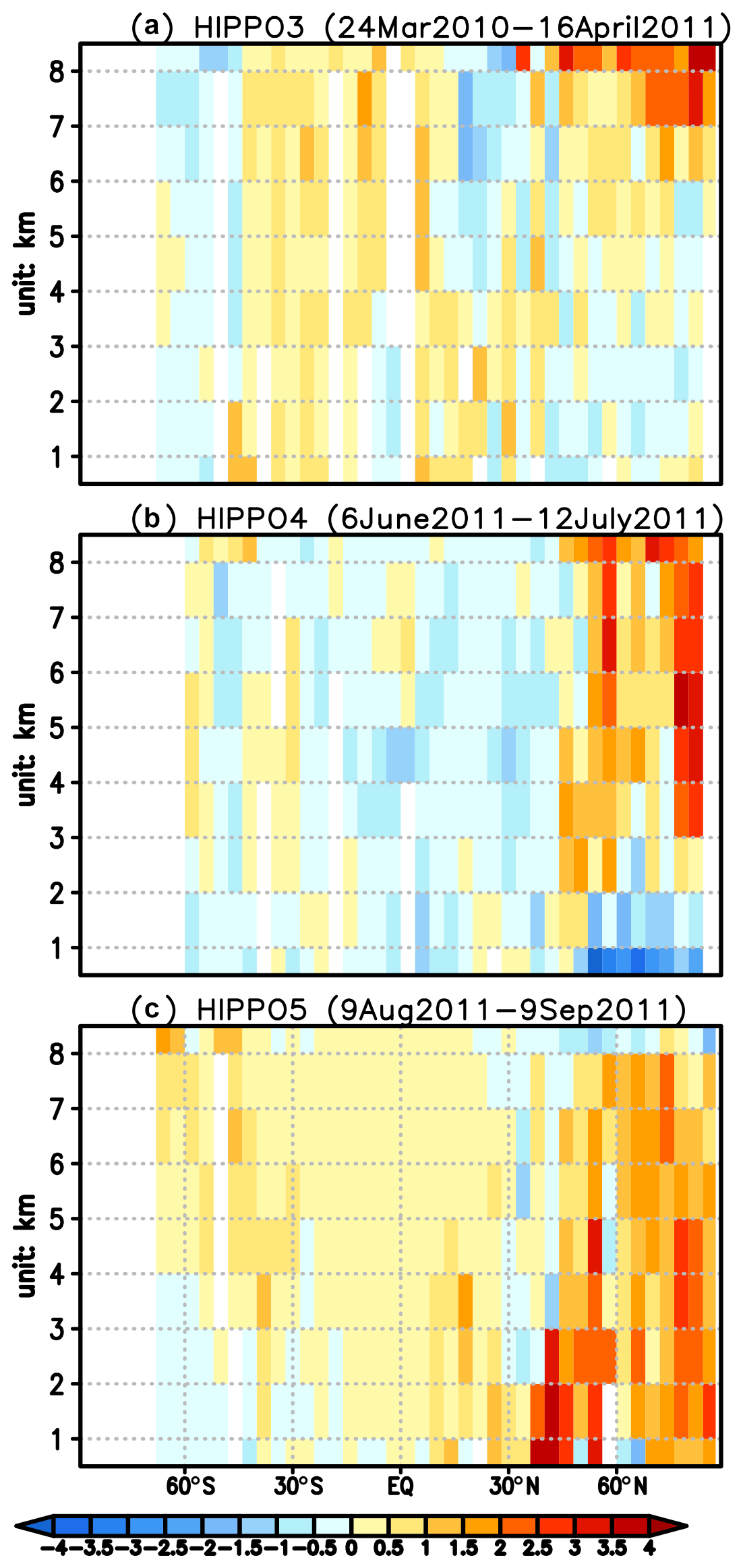
Figure B7 Differences between posterior CO₂ and HIPPO 3–5 aircraft CO₂ observations over the Pacific (A–C) as a function of latitude and altitude. Unit: ppm.

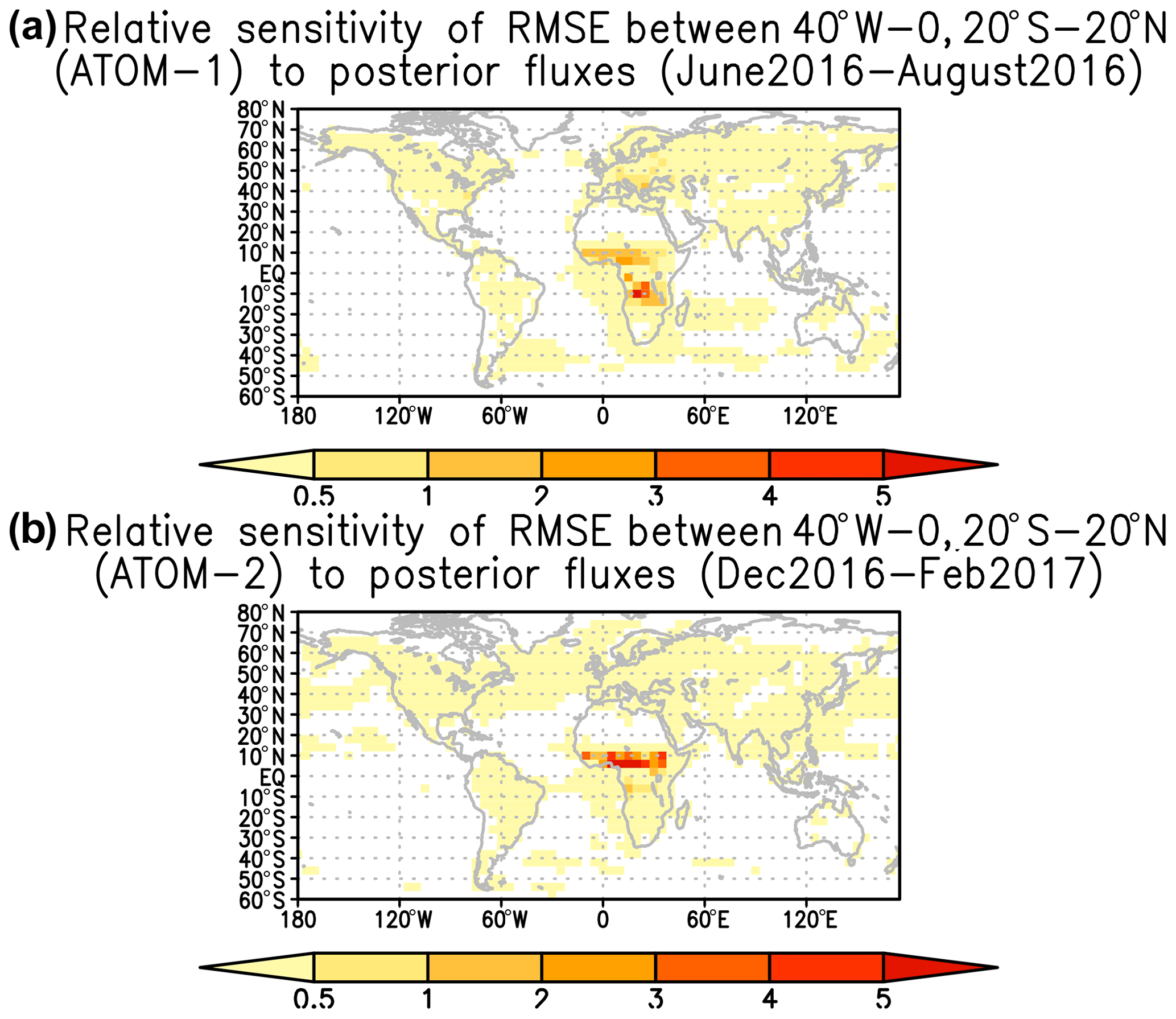
Figure B8 The relative sensitivity of RMSE of posterior CO₂ to NBE over land and air–sea net carbon exchange over ocean at every grid point. The RMSE is calculated against aircraft CO₂ observations from ATom 1 (a) and ATom 2 (b) between 40^∘ W–0^∘, 20^∘ S–20^∘ N. The adjoint model is carried out over June–August 2016 (a) and December 2016–February 2017 (b). Unit: %.

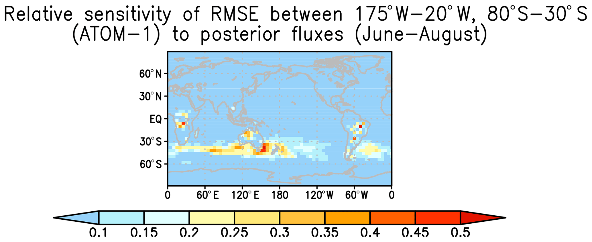
Figure B9 The relative sensitivity of RMSE of posterior CO₂ to NBE over land and air–sea net carbon exchange over ocean at every grid point. The RMSE is calculated against aircraft CO₂ observations from ATom 1 between 175–20^∘ W, 80–30^∘ S. The adjoint model is carried out over June–August 2016. Unit: %.

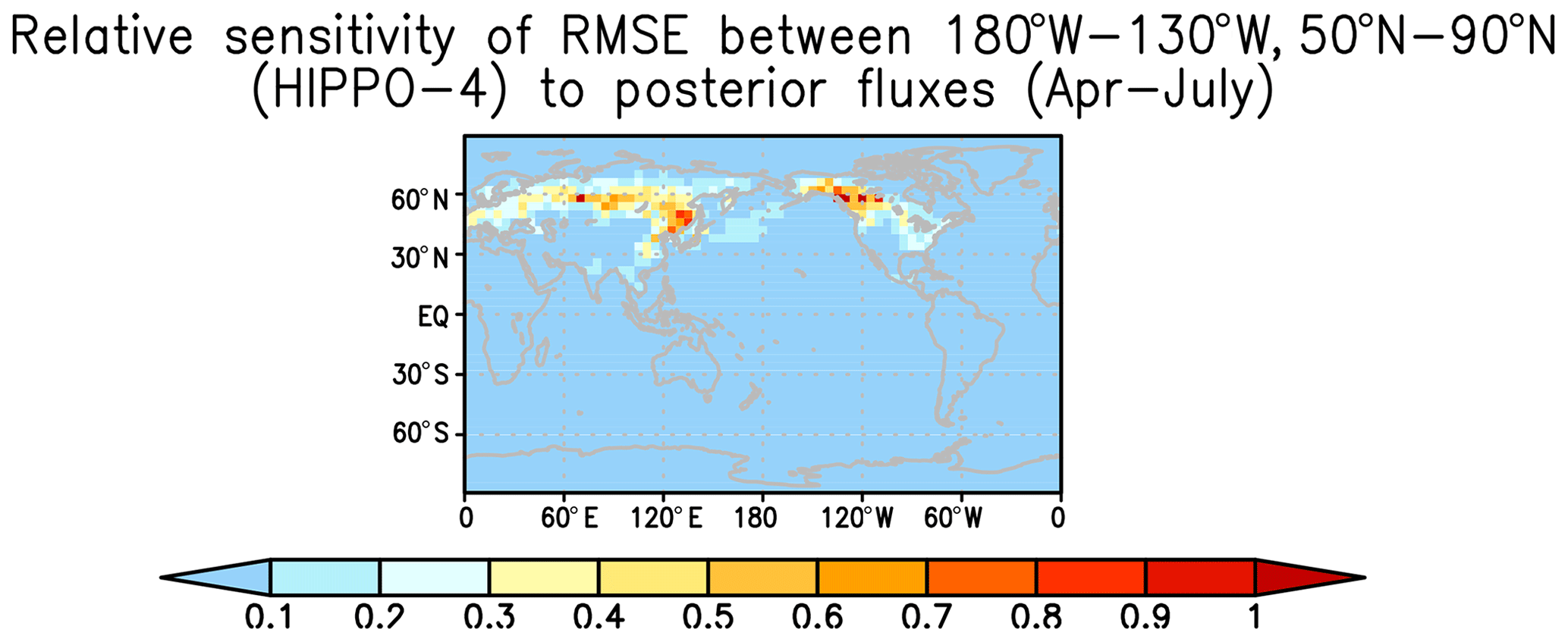
Figure B10 The relative sensitivity of RMSE of posterior CO₂ to NBE over land and air–sea net carbon exchange over ocean at every grid point. The RMSE is calculated against aircraft CO₂ observations from HIPPO 4 between 180–130^∘ W, 50–90^∘ N. The adjoint model is carried out over April–July 2011. Unit: %.

Figure B11 Monthly posterior air–sea CO₂ exchanges between 85–30^∘ S. Unit: g C/m²/d.