CLIGEN parameter regionalization for mainland China

The stochastic weather generator CLIGEN can simulate long-term weather sequences as input to WEPP for erosion predictions. Its use, however, has been somewhat restricted by limited observations at high spatial–temporal resolutions. Long-term daily temperature, daily, and hourly precipitation data from 2405 stations and daily solar radiation from 130 stations distributed across mainland China were collected to develop the most critical set of site-specific parameter values for CLIGEN. Ordinary kriging (OK) and universal kriging (UK) with auxiliary covariables, i.e., longitude, latitude, elevation, and the mean annual rainfall, were used to interpolate parameter values into a 10 km×10 km grid, and the interpolation accuracy was evaluated based on the leave-one-out cross-validation. Results showed that UK generally outperformed OK. The root mean square error between UK-interpolated and observed temperature-related parameters was ≤0.88 ^∘C (1.58 ^∘F). The Nash–Sutcliffe efficiency coefficient for precipitation- and solar-radiation-related parameters was ≥0.87, except for the skewness coefficient of daily precipitation, which was 0.78. In addition, CLIGEN-simulated daily weather sequences using UK-interpolated and observed parameters showed consistent statistics and frequency distributions. The mean absolute discrepancy between the two sequences for temperature was <0.51 ^∘C, and the mean absolute relative discrepancy for solar radiation, precipitation amount, duration, and maximum 30 min intensity was <5 % in terms of the mean and standard deviation. These CLIGEN parameter values at 10 km resolution would meet the minimum data requirements for WEPP application throughout mainland China. The dataset is available at http://clicia.bnu.edu.cn/data/cligen.html (last access: 20 May 2021) and https://doi.org/10.12275/bnu.clicia.CLIGEN.CN.gridinput.001 (Wang et al., 2020).

1 Introduction

Weather generators (WGs) are stochastic models that can generate arbitrarily long sequences of weather variables with statistical properties that are similar to observations for a specific location or area (Yin and Chen, 2020). Early WGs were originally developed to provide surrogate climate series for hydrological, soil erosion, and agricultural models when the observed data could not satisfy the application requirements due to missing data, limited record length, or spatial coverage (Wilks and Wilby, 1999). Since the 1990s, WGs have received increased attention as a statistical downscaling tool for the assessment of climate change impact (Katz and Parlange, 1996; Maraun et al., 2010). While global climate models (GCMs)/regional climate models (RCMs) have been used for climate projections, outputs from these models were often too coarse to meet the requirements of earth surface process models in terms of spatial–temporal resolutions and were biased compared with observations. Statistical downscaling methods, mainly including perfect prognosis (PP), model output statistics (MOS), and WGs, can be used to downscale and bias-correct the output from GCMs/RCMs prior to earth surface model applications (Maraun and Widmann, 2018; Yin and Chen, 2020).

CLIGEN is a stochastic WG developed based on the generators used in the EPIC and SWRRB models (Williams et al., 1985, 1984) and was released in 1995, initially accompanying the process-based Water Erosion Prediction Project (WEPP) model from the United States Department of Agriculture (Nicks et al., 1995). CLIGEN can simulate a series of long-term climate data in daily scale, including maximum and minimum temperatures, precipitation, solar radiation, dew point, wind velocity, and direction. In addition, CLIGEN can generate three inter-storm variables in sub-daily scale, including storm duration, time to peak intensity (t_p), and the ratio of the peak intensity to the average intensity (i_p), from which an unlimited length of high-resolution breakpoint data can be generated (Flanagan et al., 2001; Nicks et al., 1995; Yu, 2003).

Of the 10 CLIGEN-simulated weather elements, seven, namely daily maximum and minimum temperature, daily precipitation, duration, t_p, i_p, and daily solar radiation, are all that are required for predicting hydrological processes, soil erosion, and bio-production (Arnold et al., 1998; Flanagan et al., 2001; USDA-ARS, 2013; Wallis and Griffiths, 1995). These seven climate elements are considered to meet the minimum data requirements for WEPP. As CLIGEN is independent of WEPP, it can be used to provide simulated climate series for other surface process models as well (Flanagan et al., 2014; Yu, 2002).

Table 1 Summary of CLIGEN input parameters and the data used for the calculation of parameters.

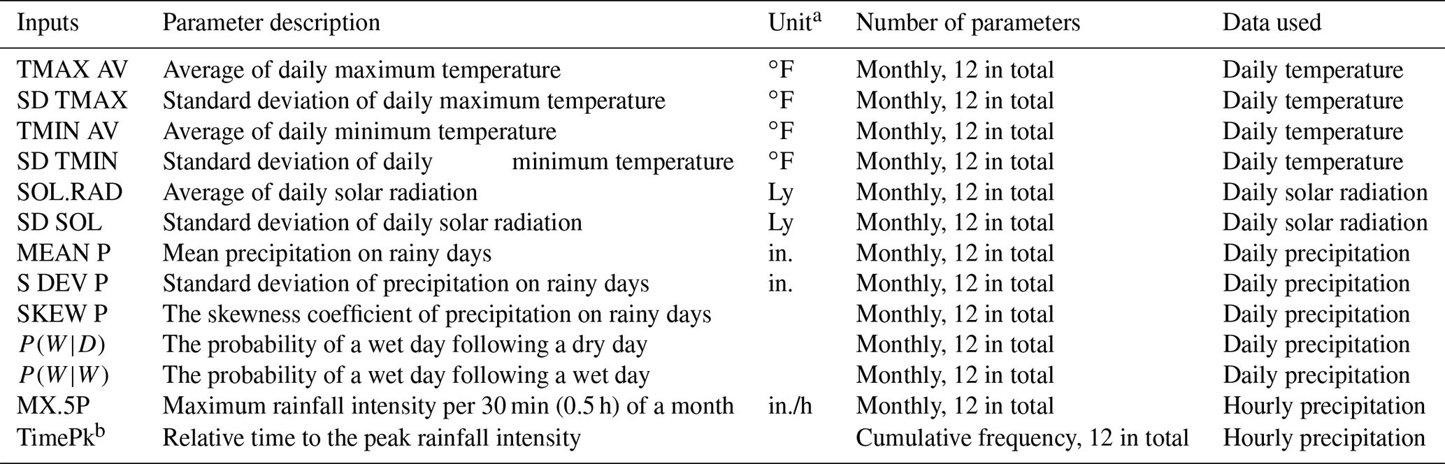
^a CLIGEN input parameter values are required to have a US customary unit. ^b The 12th parameter of TimePk for all stations is equal to 1.

Thirteen groups of input parameters related to temperature, solar radiation, and precipitation as listed in Table 1 are all parameters needed by CLIGEN to generate the aforementioned seven climate elements. As a site-specific weather generator, input parameters for CLIGEN can be directly prepared for stations with observed data. CLIGEN was initially released in the United States with a set of 2600 weather station parameter files (Flanagan et al., 2001). Parameters for the daily temperature and daily precipitation were calculated directly based on the observations of temperature and precipitation from each station. Parameters for daily solar radiation and storm pattern were based on 142 weather stations with daily solar radiation and sub-daily rainfall observations first and then extended to 2000 other stations using the triangulation interpolation method (Scheele and Hall, 2000).

Parameter regionalization, which extends model parameter values from stations with observations to areas/regions without observations, is required when the model is going to be used in these areas/regions. Commonly used parameter regionalization methods can be categorized as follows: (1) the parametric transplantation method, where a reference area that is spatially near or has similar climate characteristics to the target area is first selected, and then the parameters of the reference area are extended to the target area (Cheng et al., 2016); (2) spatial interpolation methods such as Thiessen polygon, inverse distance weighted, or ordinary kriging, which interpolate parameter values based on spatial correlations of parameters among multiple stations (Hutchinson, 1995); (3) parameter transfer as a function of regional properties such as multiple regression, based on correlations between parameters and regional characteristics (Cowpertwait et al., 1996); (4) regionalization considering both the spatial correlation of parameters and the correlation between parameters and regional characteristics, including external drift kriging and universal kriging that can be treated as combination methods to take advantage of method (2) and (3) (Haberlandt, 1998; Semenov and Brooks, 1999).

The accuracy of parameter regionalization is known to be influenced by several factors. Firstly, regionalization of climate variables with lower or regular spatial variability generally performs better than highly heterogeneous and discontinuous variables. Secondly, for the same climate variable, temporal resolution plays an important role. The climate variable at a monthly or annual scale tends to perform better than variables at a daily or hourly scale because data with finer resolutions possess greater spatial variability. Thirdly, adopted approaches affect the efficiency of regionalization. For example, Wilks (2008) compared and evaluated the interpolation accuracy of four spatial interpolation methods for parameters of WGEN (weather generator), a weather generator developed by Richardson and Wright (1984), and results showed that locally weighted regressions outperformed Thiessen polygons and domain-wide (“global”) regressions. The accuracy of interpolation can be improved by adopting auxiliary covariables that are correlated with the regionalized climate variables into the regionalization process (Hengl et al., 2007). For example, elevation is frequently used as an auxiliary covariable and has been found to improve the interpolation of temperature and precipitation (Carrera-Hernández and Gaskin, 2007; Ly et al., 2013; Verworn and Haberlandt, 2011), especially in mountainous regions with complex terrains (Xu et al., 2018).

Several studies have been attempted at regionalization of CLIGEN input parameters. Regionalization of CLIGEN input parameters for WEPP has combined the parametric transplantation and spatial interpolation. When CLIGEN was developed in the United States to provide climate input to WEPP, parameter values for 2600 stations were regionalized based on inverse distance weighting (IDW). In the WEPP application, users identify the targeted location, for which daily weather sequences using parameters from the nearest stations will be automatically generated directly or by interpolation from surrounding stations (up to 20 stations within a distance of 1^∘ of latitude/longitude). The parameter files and the internally installed interpolation in the WEPP application have facilitated the application of CLIGEN/WEPP in the United States. However, the accuracy of regionalized parameters has not been evaluated, and the effect on generated weather sequences using the interpolated parameters is largely unknown.

Chen (2008) explored four spatial interpolation methods, inverse distance weighting (IDW), ordinary kriging (OK), global polynomial interpolation (GPI), and local polynomial interpolation (LPI), to regionalize the daily temperature- and precipitation-related input parameters of CLIGEN for 12 stations in the Loess Plateau of China. Paired t tests showed that the temperature and precipitation series generated using interpolated input parameters were not significantly different from those generated using input parameters computed using observations for the 12 stations considered (Chen, 2008). However, solar-radiation- and storm-pattern-related parameters used to generate daily solar radiation and storm characteristics were not considered in Chen's study (Chen, 2008). Input parameters for simulating the seven weather variables mentioned above, listed in Table 1, meet the minimum data requirements for WEPP at a specific station. Without solar-radiation- and storm-pattern-related parameter values, CLIGEN cannot be used to generate the required weather sequences for WEPP.

The overall aim of this study was to enable widespread use of CLIGEN to generate daily temperature, solar radiation, precipitation, and sub-daily precipitation variables anywhere in mainland China and to gain better understanding of the performance of various spatial interpretation techniques. Specific objectives of this study were to (1) assemble CLIGEN input parameter values for 2405 stations in mainland China based on meteorological observations; (2) evaluate spatial interpolation techniques for regionalizing CLIGEN parameters; and (3) produce grid-based CLIGEN temperature, solar radiation, and precipitation parameter values at 10 km resolution for mainland China.

Table 2 Data lengths for daily temperature, daily and hourly precipitation, and daily solar radiation for stations used in this study.

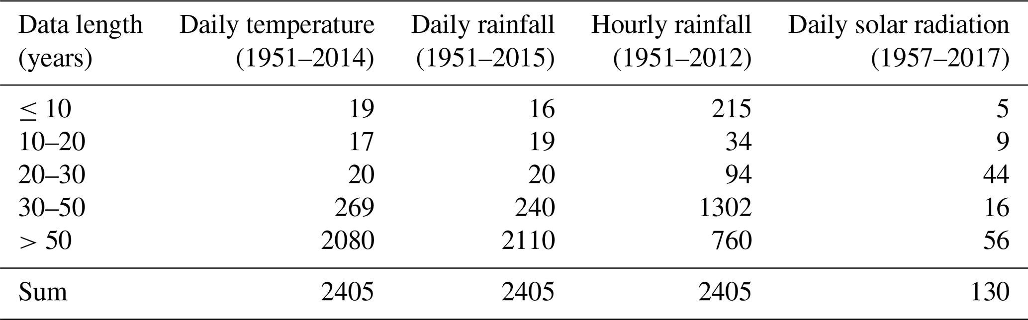
Figure 1 Map of the study area showing the locations of meteorological stations used in this study.

2 Data and methods

2.1 Data collection

Four datasets consisting of daily temperature, daily rainfall, and hourly rainfall from 2405 meteorological stations, as well as solar radiation data from 130 stations distributed across mainland China, were collected (Fig. 1) from the National Meteorological Information Center (NMIC) of the China Meteorological Administration (CMA) and have been quality controlled by NMIC. Data lengths were different for these four datasets (Table 2). Daily temperature and daily rainfall data were characterized by longer periods of observation for most stations compared with hourly rainfall data, especially for stations located in the northwest arid area and the Qinghai–Tibet Plateau where gauges for observing hourly rainfall for some stations were installed very late (Zhao, 1983; Wang and Zuo, 2009). Based on these four datasets, a total of 156 parameter values were calculated for each station. It should be noted that the 12th value of TimePk is equal to 1 by definition, and 155 parameters were involved in the calculation and interpolation. The siphon rain gauges used to record hourly rainfall were stopped in winter to avoid freezing failures; therefore, hourly rainfall was only available for the warm rainy season for some northern and western stations. Nine stations distributed in North China (Miyun, Zhengzhou, Harbin), Northwest China (Lanzhou, Ürümqi), the Tibetan Plateau (Lhasa), and South China (Fuzhou, Changsha, Haikou) were selected to further display the regional differences and monthly variability of input parameters (Fig. 1).

2.2 Site-based input parameters and simulation

CLIGEN requires 13 groups of input parameters and 12 values for each group to stochastically simulate temperature, solar radiation, and precipitation (Table 1). Temperature-related input parameters, TMAX AV, SD TMAX, TMIN AV, and SD TMIN, are used to simulate the daily maximum and minimum temperature for each simulated day and to decide whether the simulated precipitation occurred as snowfall or rainfall (Table 1). These four values can be calculated using daily maximum and minimum temperature data for each month directly. Solar-radiation-related inputs SOL.RAD and SD SOL are used to generate daily solar radiation and can be directly obtained from observed daily solar radiation.

The wet-following-wet and wet-following-dry day transition probabilities, P(W|D) and P(W|W), are used to determine the occurrence of rainy days with a first-order two-states Markov chain prepared as follows:

$$\begin{array}{}\text{(1)}& {\displaystyle }P\left(W\mathrm{|}W\right)={\displaystyle \frac{N_{\mathrm{ww}}}{N_{\mathrm{wd}}+N_{\mathrm{ww}}}},\text{(2)}& {\displaystyle }P\left(W\mathrm{|}D\right)={\displaystyle \frac{N_{\mathrm{dw}}}{N_{\mathrm{dw}}+N_{\mathrm{dd}}}},\end{array}$$

in which N_ww, N_wd, N_dw, and N_dd represent the number of days in a month that a wet day followed a wet day, a wet day followed a dry day, a dry day followed a wet day, and a dry day followed a dry day, respectively. For each simulated wet day, MEAN P, S DEV P, and SKEW P are used to simulate the daily precipitation amount using a skewness normal distribution. These three parameters can be computed directly from daily precipitation month by month. As CLIGEN assumes there is only one storm occurring on a wet day, daily precipitation depths in CLIGEN are equal to storm precipitation amount.

MX.5P and TimePk are used to simulate inter-storm variables, including storm duration (D, h) and two normalized dimensionless variables, the ratio of peak intensity to average intensity (i_p), and the ratio of time to the peak intensity to storm duration (t_p) (Nicks et al., 1995; Yu, 2002; Yu, 2003; Zhang and Garbrecht, 2003). MX.5P represents the average maximum 30 min intensity for each month. The maximum 30 min intensity for a wet day is denoted as I₃₀. If a month has n wet days, the maximum I₃₀ among n wet days can be denoted by maxI₃₀; and for a specific month in a data series of k years, the MX.5P is given by

$$\begin{array}{}\text{(3)}& \mathrm{MX}.5\mathrm{P}={\displaystyle \frac{\mathrm{1}}{k}}\sum \max I_{\mathrm{30}}.\end{array}$$

Ideally, MX.5P values should be prepared using rainfall data with a resolution of 30 min or less. Depending on the temporal resolution, I₃₀ can be calculated directly from moving averages of the original data over successive 30 min. Given the limited availability of high-resolution rainfall observations for this study, MX.5P was estimated using hourly data described in detail elsewhere (Wang et al., 2018).

In CLIGEN (Nicks et al., 1995), as in Arnold and Williams (1989), it is assumed that the magnitude of precipitation intensity decreases exponentially from the maximum rate when time distribution of precipitation intensities is discarded. Therefore, the precipitation depth P_Δt in any given interval Δt can be described by

$$\begin{array}{}\text{(4)}& P_{\mathrm{\Delta }t}=i_{\mathrm{p}}\underset{\mathrm{0}}{\overset{\mathrm{\Delta }t}{\int }}{e}^{-t/\mathit{\tau }}\mathrm{d}t=\mathit{\tau }{i}_{\mathrm{p}}\left(\mathrm{1}-e^{-\mathrm{\Delta }t/\mathit{\tau }}\right).\end{array}$$

For hourly data, the interval Δt=1 h, and the maximum 1 h precipitation P_1 h and maximum 2 h precipitation P_2 h were known:

$$\begin{array}{}\text{(5)}& {\displaystyle \frac{P_{\mathrm{1}\mathrm{h}}}{P_{\mathrm{2}\mathrm{h}}}}={\displaystyle \frac{\mathrm{1}-e^{-\mathrm{1}/\mathit{\tau }}}{\mathrm{1}-e^{-\mathrm{2}/\mathit{\tau }}}},\end{array}$$

where τ can be solved and then i_p can be readily obtained as

$$\begin{array}{}\text{(6)}& i_{\mathrm{p}}={\displaystyle \frac{P_{\mathrm{1}\mathrm{h}}}{\mathit{\tau }(\mathrm{1}-e^{-\frac{\mathrm{1}}{\mathit{\tau }}})}}.\end{array}$$

Once τ and i_p are known, the maximum 30 min precipitation P_0.5 can be determined as

$$\begin{array}{}\text{(7)}& P_{\mathrm{0.5}\mathrm{h}}=\mathit{\tau }{i}_{\mathrm{p}}(\mathrm{1}-e^{-\frac{\mathrm{1}}{\mathrm{2}\mathit{\tau }}}).\end{array}$$

The maximum 30 min rainfall intensity is given simply as

$$\begin{array}{}\text{(8)}& I_{\mathrm{30}\min }=\mathrm{2}{P}_{\mathrm{0.5}\mathrm{h}}.\end{array}$$

In reference to Wang et al. (2018), MX.5P can be directly prepared using hourly rainfall data.

There are 12 discrete values of TimePk for each station, describing an empirical cumulative probability distribution of time to peak (Nicks et al., 1995). The observed interval is Δt, and the storm duration, D, consists of n intervals. If the peak intensity occurs in the ith interval, time to peak intensity, T_p, is estimated as

$$\begin{array}{}\text{(9)}& T_{\mathrm{p}}=\left(i-{\displaystyle \frac{\mathrm{1}}{\mathrm{2}}}\right)\mathrm{\Delta }t,\end{array}$$

and time to peak as a fraction of duration is

$$\begin{array}{}\text{(10)}& t_{\mathrm{p}}={\displaystyle \frac{T_{\mathrm{p}}}{D}}={\displaystyle \frac{(i-\mathrm{0.5})}{n}}.\end{array}$$

If Nt_p(i) is the number of wet days from all data records with $t_{\mathrm{p}}\le i/\mathrm{12}$ for i=1, 2, … 12, then

$$\begin{array}{}\text{(11)}& \text{TimePk}\left(i\right)={\displaystyle \frac{N{t}_{\mathrm{p}}\left(i\right)}{N{t}_{\mathrm{p}}\left(\mathrm{12}\right)}}.\end{array}$$

TimePk computed using 1 min rainfall data and hourly rainfall data differs slightly, and it has some small influence on CLIGEN-simulated intensity and duration (Wang et al., 2018). Therefore, TimePk was prepared directly using hourly data in this study for consistency. Given the time increment (Δt) of 1 h, and known storm duration (D) for each wet day, TimePk can be computed using Eqs. (9) to (11). It is worth noting that the 12th parameter value of TimePk for all stations equals to 1 (Eq. 11).

2.3 Spatial interpolation by kriging

Kriging is a spatial interpolation method that gives the best linear unbiased prediction of intermediate values, assuming a Gaussian process governed by prior covariance. For a research region with n samples at spatial locations x_i(i=1, 2, …, n), Z(x_i) are the sample values at x_i. At an unknown target point x₀, the estimated value $\widehat{Z}\left({\mathbf{x}}_{\mathrm{0}}\right)$ can be expressed as a weighted average of the known observations Z(x_i) (Wackernagel, 2013):

$$\begin{array}{}\text{(12)}& \widehat{Z}\left({\mathbf{x}}_{\mathrm{0}}\right)=\sum _{i=\mathrm{1}}^n{\mathit{\lambda }}_{i}Z\left({\mathbf{x}}_i\right),\end{array}$$

where λ_i represents the weighting coefficients of the known sample values Z(x_i), which depend on the spatial autocorrelation structure of the sample values and should minimize the prediction error variance. Assuming the variable value Z(x) can be modeled as a combination of a deterministic trend μ(x) and an auto-correlated random error ε(x), $Z\left(\mathbf{x}\right)=\mathit{\mu }\left(\mathbf{x}\right)+\mathit{\epsilon }\left(\mathbf{x}\right)$, then the best linear unbiased prediction requires $E[\widehat{Z}\left({\mathbf{x}}_{\mathrm{0}}\right)-Z\left({\mathbf{x}}_{\mathrm{0}}\right)]=\mathrm{0}$, and Var[$\widehat{Z}\left({\mathbf{x}}_{\mathrm{0}}\right)-Z\left({\mathbf{x}}_{\mathrm{0}}\right)$] is minimized. Ordinary kriging (OK) assumes that the trend is constant but unknown, μ(x)=m, while in universal kriging (UK), the trend is assumed to be a linear combination of some known covariables f_l, $\mathit{\mu }\left(\mathbf{x}\right)=\sum _{l=\mathrm{1}}^k{\mathit{\beta }}_l{f}_l$. Universal kriging (UK) considers the relationship between the target variable and the auxiliary covariables. Soil, elevation, temperature, and remote sensing images are commonly used auxiliary covariables (Haberlandt, 1998; Li et al., 2014; McKenzie and Ryan, 1999; Semenov and Brooks, 1999).

Both OK and UK were used to interpolate the CLIGEN input parameters in this study. Stepwise regression was conducted to select appropriate covariables for UK. The longitude, latitude, elevation, and annual rainfall amount were found correlated with the parameters – one for each month for CLIGEN with the exception of the SKEW P (Table 1); therefore, all these four variables were adopted as auxiliary covariables when UK was conducted to interpolate these 12 groups of parameters. SKEW P had low correlations with all four of these covariates but good correlation with parameters MEAN P and S DEV P. Therefore, MEAN P and S DEV P were selected as covariables during the interpolation of SKEW P.

2.4 Assessment of interpolation accuracy

A leave-one-out cross-validation method was used to evaluate the interpolation accuracy of OK and UK. First, 1 of the 2405 stations was excluded from data analysis and treated as unknown, and data for the remaining 2404 stations were then used to predict parameter values for the excluded station using OK or UK. This leave-one-out procedure was repeated for 155 parameters for each of the 2405 stations (13 groups ×12 input parameters −1, as the value of the 12th parameter of TimePk is always 1, Table 1). Denoting CLIGEN parameters based on observations as P_O and the corresponding predicted CLIGEN parameters obtained using OK or UK as P_K, three indicators – root mean square error (RMSE), Nash–Sutcliffe efficiency coefficient (NSE), and percent bias (PBIAS) – were selected to evaluate and compare the performances of OK and UK as follows (Yin et al., 2019):

$$\begin{array}{}\text{(13)}& {\displaystyle }\mathrm{RMSE}=\sqrt{{\displaystyle \frac{\mathrm{1}}{n}}{\sum }_n(P_{\mathrm{O}}-P_{\mathrm{K}}{)}^{\mathrm{2}}},\text{(14)}& {\displaystyle }\mathrm{NSE}=\mathrm{1}-{\displaystyle \frac{{\sum }_n(P_{\mathrm{O}}-P_{\mathrm{K}}{)}^{\mathrm{2}}}{{\sum }_n(P_{\mathrm{O}}-\overline{P_{\mathrm{O}}}{)}^{\mathrm{2}}}},\text{(15)}& {\displaystyle }\mathrm{PBIAS}={\displaystyle \frac{{\sum }_n(P_{\mathrm{O}}-P_{\mathrm{K}})}{{\sum }_n{P}_{\mathrm{O}}}}\cdot \mathrm{100}.\end{array}$$

NSE and PBIAS are inappropriate for temperature-related parameters which are in interval scales, and the same is true of probabilities. NSE and PBIAS were computed for parameters in ratio scales only, i.e., MEAN P, S DEV P, SKEW P, SOL.RAD, and SD SOL. By calculating the above three indicators, the better of the two interpolation techniques, OK and UK, was determined and applied to calculate the regionalization of CLIGEN input parameters for mainland China. A two-dimensional grid database was established at a spatial resolution of 10 km×10 km based on the 155 sets of interpolated parameters.

Input parameters based on observed data and interpolated data using the better interpolation technique were input into CLIGEN to evaluate the influence of regionalized parameters on the simulation. For each station, 100 years of continuous climate series were generated using the default CLIGEN stochastic seed without interpolation between months, and the simulated data predicted by P_O and P_K were denoted as G_O and G_K, respectively. The maximum and minimum temperature (^∘C), daily solar radiation (langley), daily rainfall amount (mm), storm duration (h), and i_p and t_p of each simulation day were derived from G_O and G_K for each station, and the maximum 30 min intensity (I₃₀, mm/h) was calculated based on an assumed bi-exponential storm pattern (Yu, 2002). CLIGEN input parameter values are required to have a US customary unit as shown in Table 1, while CLIGEN output is produced in SI units as input to WEPP.

Three basic statistics – the average, standard deviation, and skewness coefficient – were calculated for each CLIGEN-generated variable. The absolute error (AE) and mean absolute error (MAE) were calculated to examine the differences between the two sets of statistics for generated temperatures. Relative error (RE) and mean absolute relative error (MARE) were calculated to examine the differences between the two sets of statistics for generated daily solar radiation, daily precipitation, and sub-daily storm pattern:

$$\begin{array}{}\text{(16)}& {\displaystyle }\left|\text{AE}\right|=\mathrm{|}{G}_{\mathrm{O}}-G_{\mathrm{K}}\mathrm{|},\text{(17)}& {\displaystyle }\text{MAE}={\displaystyle \frac{\mathrm{1}}{\mathrm{2405}}}\sum \left|(G_{\mathrm{O}}-G_{\mathrm{K}})\right|,\text{(18)}& {\displaystyle }\mathrm{|}\text{RE}\mathrm{|}=\mathrm{100}\mathit{\%}\mathrm{|}(G_{\mathrm{O}}-G_{\mathrm{K}})/G_O\mathrm{|},\text{(19)}& {\displaystyle }\mathrm{MARE}={\displaystyle \frac{\mathrm{100}\mathit{\%}}{\mathrm{2405}}}\sum \left|(G_{\mathrm{O}}-G_{\mathrm{K}})/G_{\mathrm{O}}\right|.\end{array}$$

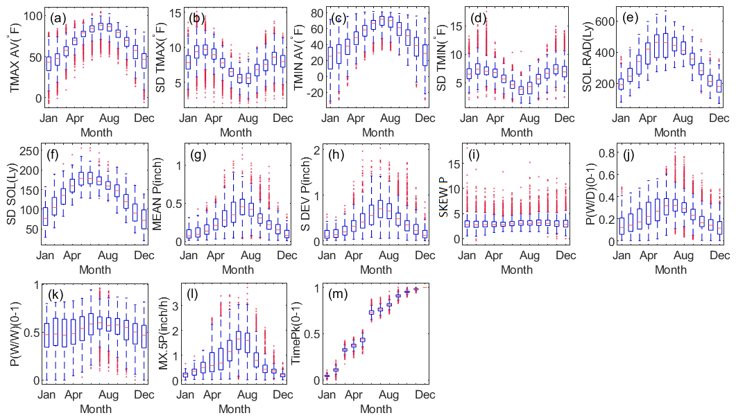
Figure 2 Boxplot of CLIGEN temperature, solar radiation, and precipitation parameters obtained from observations in mainland China.

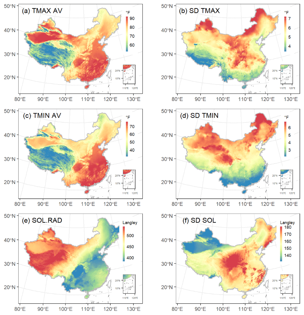
Figure 3 Map of the study area showing the spatial distribution of CLIGEN temperature-related parameters of mainland China in August. All parameters were regionalized using universal kriging.

3 Results

3.1 Spatial–temporal distribution of CLIGEN input parameters

Thirteen groups of CLIGEN temperature and precipitation parameters from 2405 stations and solar radiation parameters from 130 stations were plotted to examine the inter-annual variation and the differences among parameters (Fig. 2). The average maximum temperature and minimum temperature, TMAX AV and TMIN AV (in unit of ^∘F, 1 ^∘F = 1 ^∘C $/$ 1.8+32), and the average and standard deviation of solar radiation, SOL.RAD and SD SOL (in unit of langley, 1 Ly = $\mathrm{4.184}\times {\mathrm{10}}^{-\mathrm{2}}$ MJ/m²), showed strong seasonality, and the spatial variance became smaller from the cold season to the warm one (Fig. 2a, c, e–f). The spatial distributions of CLIGEN temperatures and solar-radiation-related inputs in August based on the UK-interpolated results were depicted as examples (Fig. 3), from which we can find a differentiation rule for latitude and vertical zonality for TMAX AV and TMIN AV (Fig. 3a and c). SD TMAX and SD TMIN varied with season with a similar pattern and with generally higher values in spring and autumn (Fig. 2b and d), because these two seasons are transitional periods between warm and cold seasons when temperature fluctuations are larger.

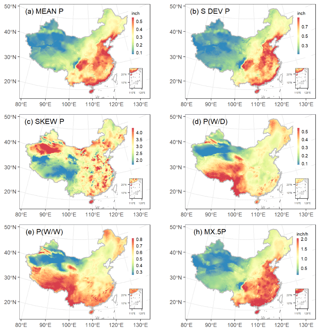
Figure 4 Map of the study area showing the spatial distribution of CLIGEN precipitation-related parameters of mainland China in August. All parameters were regionalized using universal kriging.

The average and standard deviation of daily precipitation, MEAN P and S DEV P (in inches, 1 in. = 25.4 mm), and the average monthly maximum 30 min intensity, MX.5P (in unit of in./h, 1 in./h = 25.4 mm/h), showed a similar seasonal pattern with the parameter values becoming gradually higher from the cold season to the warm (Fig. 2g–h and l). Precipitation in China is influenced by the East Asian summer monsoon and the location relative to land and sea. From the spatial distribution of daily precipitation in August we found a general decreasing trend from southeast to southwest (Fig. 4a–b). The August rain belt is located in North and Northeast China, while the South China region is controlled by the subtropical high-pressure belt and experiences a summer drought. Therefore, MEAN P and MX.5P in North China were apparently greater than in South China. In comparison, skewness of daily precipitation, SKEW P, showed imperceptible differences among months and no apparent latitudinal or longitudinal zonality (Fig. 4c). This may be one of the reasons leading to the low spatial interpolation accuracy of SKEW P.

The wet-following-dry transition probability P(W|D) showed a clear inter-annual variability in that the probability increased from cold season to warm (Fig. 2j), while the wet-following-wet transition probability P(W|W) was characterized by greater regional differences but smaller monthly variability for most stations compared with P(W|D) (Fig. 2k). The spatial–temporal variation in these two transition probabilities revealed the stepwise northward progress of the East Asian monsoon and the north–south advance of the frontal cyclone (Liao et al., 2004). Due to the pre-monsoon rainy season before June, strong convection in summer, and the retreating monsoon rain belt after August, the southern region was characterized by a longer rainy season than North China (Yu and Zhou, 2007). Therefore, P(W|W) of the southern region was generally higher than other regions, and its seasonal variations were relatively insignificant (Fig. 5b).

Figure 5 P(W|D), P(W|W), MX.5P, and TimePk of nine stations determined by observed daily precipitation.

MX.5P of nine example stations showed the regional differences more clearly in that the parameters of southern stations were relatively higher (Fig. 5c). Differences among southern and northern stations became gradually smaller in the warm season. It should be noted that the narrower range of MX.5P in winter was partially related to the limited availability of hourly data. Due to the restriction of low temperatures on siphon rain gauge observations, MX.5P in cold seasons was available for fewer stations than in warm seasons.

TimePk consists of 12 discrete values representing the cumulative distribution of time to peak intensity ranging from 0 to 1 for a specific location. The sixth value for TimePk represents the cumulative ratio of storms with peak intensity occurring before $\mathrm{1}/\mathrm{2}$ duration and related ratios for 2405 stations ranging from 60 % to 80 % (Fig. 2m). TimePk for nine example stations shows the cumulative ratio of time to peak intensity in different regions, consistently indicating that most peak intensities tend to occur earlier during the storms, with no obvious regional differences found for this parameter (Fig. 5d).

Table 3 Comparison of the accuracy of OK and UK using the leave-one-out cross-validation.

^a Overall average (AV) and ^b standard deviation (SD) for all months and stations; the unit is identical with parameters. ^c The unit of RMSE is identical with the unit of each group of parameters. ^d NSE and PBIAS were only calculated for parameters in the ratio scale with true zero.

3.2 Evaluation of interpolated parameters using OK and UK

3.2.1 Parameters at the daily scale

The leave-one-out cross-validation showed that four groups of temperature parameters (TMAX AV, SD TMAX, TMIN AV, SD TMIN), two groups of solar radiation (SOL.RAD, SD SOL), and four groups of precipitation parameters at a daily scale (MEAN P, S DEV P, P(W|D), and P(W|W)) were well predicted by ordinary kriging (OK) and universal kriging (UK). RMSE for all these parameters were relatively low compared with the average of observed inputs (Table 3). For all these four groups of temperature-related parameters, RMSE values between the UK-interpolated and observed were less than ≤1.58 ^∘F (0.88 ^∘C). NSE values were greater than 0.87 for parameters of MEAN P, S DEV P, SOL.RAD, and SD SOL in ratio scales. The PBIAS values were all smaller than 1 %, suggesting that parameters based on observation and interpolation have a very close average trend and showed no obvious bias. In contrast, the interpolated accuracy of the skewness coefficient of daily precipitation, SKEW P, was not very satisfactory, with NSE being 0.48 using OK and 0.78 using UK. Parameters related to daily average (TMAX AV, TMIN AV, SOL.RAD, and MEAN P) were generally better predicted than corresponding parameters related to standard deviation (SD TMAX, SD TMIN, SD SOL, and S DEV P), and the skewness coefficient was the least accurately simulated.

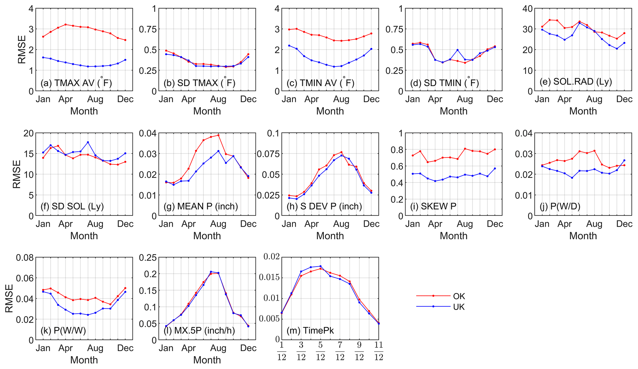
Figure 6 Comparison of the interpolation quality in terms of the root mean square error (RMSE) using ordinary kriging (OK) and universal kriging (UK) for temperature, solar radiation, and precipitation parameters.

In comparison with OK, the overall and monthly predicted accuracy using UK with auxiliary covariables obviously improved TMAX AV, TMIN AV, SOL.RAD, MEAN P, SKEW P, P(W|W), and P(W|D) (Fig. 6). The predicted accuracy for SD TMAX and S DEV P using the two techniques showed no evident difference. For SD TMIN and SD SOL, the predicted accuracies were approximate except for July, when the RMSE values of UK were obviously larger than those of OK and the reason was unclear. Although the prediction of SKEW P using UK was not as good as other parameters at a daily scale, the improvement compared with OK was quite obvious, as the NSE over 12 months increased from 0.48 for OK to 0.78 for UK, and the RMSE decreased from 0.73 to 0.47 mm (Table 3). Predicted inputs using OK and UK versus inputs based on observations from August were plotted to show the difference between two methods as examples (Fig. 7a–k).

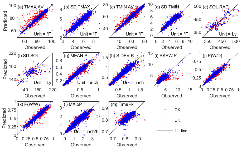
Figure 7 Comparison of the interpolation quality using ordinary kriging (OK) and universal kriging (UK) for CLIGEN temperature, solar radiation, and precipitation parameters in August, and the eighth parameter of TimePk.

3.2.2 Parameters at the sub-daily scale

Cross-validation results showed that the interpolation of the two parameters related to storm patterns, i.e., MX.5P and TimePk, performed well. Three cross-validation statistics for these two parameters using two methods were numerically similar (Table 3). NSE over 12 months for MX.5P interpolated with OK and UK were both equal to 0.95. The seasonal variation in RMSE based on OK and UK follows a similar pattern (Fig. 6l–m). For TimePk, the RMSE values using OK were slightly lower than those using UK for the third, fourth, and fifth parameters but slightly higher for the others.

Interpolation accuracy has been adequately estimated through cross-validation, and these results indicated that the accuracy of interpolation results based on UK was generally higher than those based on OK. Therefore, two sets of CLIGEN-simulated climate series using observed inputs and UK-interpolated inputs were generated and compared to further evaluate the regionalized parameters using UK for the simulation of CLIGEN.

Table 4 Comparison of CLIGEN generated daily temperature and solar radiation based on observed input parameters and UK-interpolated ones.

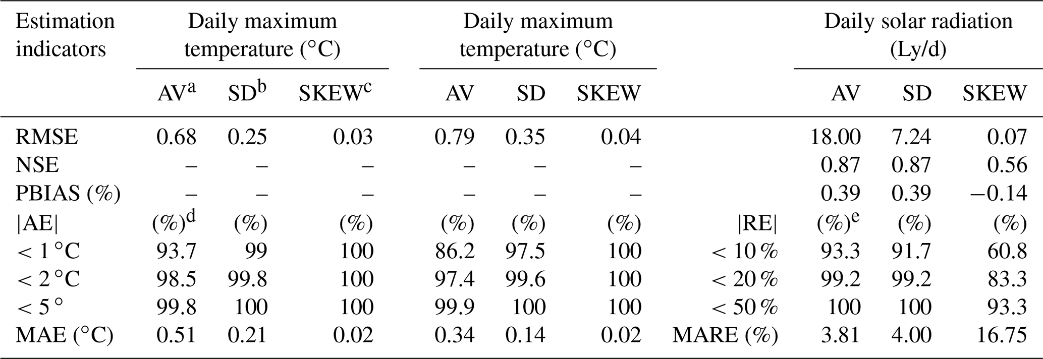
^a The average (AV), ^b the standard deviation (SD), and ^c the skewness coefficient (SKEW) of daily maximum/minimum temperature and solar radiation simulated by CLIGEN. ^d Percent of stations with |AE| in a range. ^e Percent of stations with |RE| in a range.

Table 5 Comparison of CLIGEN-generated daily rainfall and annual rainy days based on observed input parameters and UK-interpolated ones.

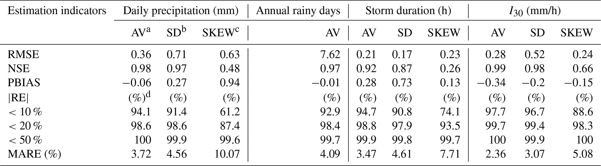
^a The average (AV), ^b the standard deviation (SD), and ^c the skewness coefficient (SKEW) of daily precipitation, annual rainy days, storm duration, and I₃₀ by CLIGEN. ^d Percent of stations with |RE| in a range.

3.3 Assessment of parameters' regionalization on the CLIGEN outputs

3.3.1 Simulated climate elements at a daily scale

CLIGEN-simulated daily temperature and solar radiation based on UK-interpolated input parameters agreed well with those simulated based on observed parameters. The average, standard deviation, and skewness coefficient of generated daily maximum temperature, minimum temperature, solar radiation, and daily precipitation generated using observed and interpolated input parameters were calculated for each station, and the simulated accuracies of the average and standard deviation were found to be better than that of the skewness coefficient. The RMSE of the mean and standard deviation were all less than 0.79^∘C, 18 Ly/d (0.75 MJ/d), and 0.71 mm, respectively, for daily temperatures, solar radiation, and precipitation (Tables 4 and 5). The NSE of the skewness coefficient for solar radiation was 0.56, obviously lower than that for the mean and standard deviation (Table 4). Meanwhile, the NSE of the skewness coefficient of daily precipitation was low (Table 5), indicating a relatively low interpolation accuracy of SKEW P. In fact, the accuracy of SKEW P was the lowest among all input parameters (Table 3).

The absolute error (AE) of the average, standard deviation, and skewness coefficient between the simulated daily temperature of G_O and G_K were statistically similar (Table 4). The mean absolute error (MAE) over 2405 stations were all lower than 0.51 ^∘C. For daily solar radiation, the relative errors (REs) for the mean and standard deviation were lower than 10 % for more than 90 % stations, and the mean absolute relative error (MARE) values were lower than 4 %.

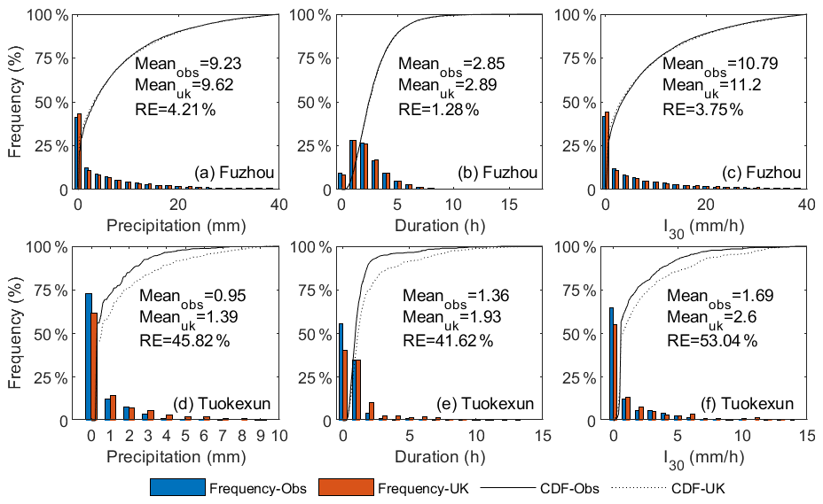
Figure 8 Frequency distribution of daily precipitation, duration, and maximum 30 min intensity (I₃₀) generated by CLIGEN using inputs based on observations and interpolation predicted parameters: Fuzhou station (a–c) and Tuokexun station (d–f) as examples.

For generated daily precipitation, 94.1 % and 91.4 % of stations yielded RE of the average and standard deviation below 10 %, and the MARE values for 2405 stations were 3.72 % and 4.56 %, respectively. The bias between annual rainy days of G_O and G_K was small as well. RE values of 92.9 % of stations were lower than 10 %. The frequency distributions of daily precipitation generated using two sets of inputs were well matched for most stations. Figure 8a depicted the frequency distributions of simulated daily precipitation for Fuzhou station as an example, with RE slightly higher than MARE over 2405 stations. Meanwhile, some stations do not satisfactorily simulate the frequency distribution. The frequency distribution of Tuokexun, whose simulation quality was approximately the worst among 2405 stations, was offered as an example (Fig. 8d). It showed that the frequency of daily precipitation ranging from 0–1 mm was underestimated, whereas that for values greater than 1 mm was overestimated (Fig. 8d).

3.3.2 Simulated storm-pattern-related variables

The average and standard deviation of storm duration and the maximum 30 min intensity (I₃₀) generated using observed and UK-interpolated input parameters possessed a generally small bias. The NSE of the average and standard deviation for both duration and I₃₀ were above 0.87. Compared with the average and standard deviation, the accuracy of skewness was the worst, with the NSE being 0.26 for the duration and 0.66 for the peak intensity index. Comparison of the frequency distribution of the duration and I₃₀ for Fuzhou station showed that the frequency of simulated storm patterns was well preserved using data employing UK-interpolated parameters (Fig. 8b–c). The frequency distribution of the duration and I₃₀ for Tuokexun station showed that interpolated parameters seemed to underestimate low values and overestimate high values (Fig. 8e–f).

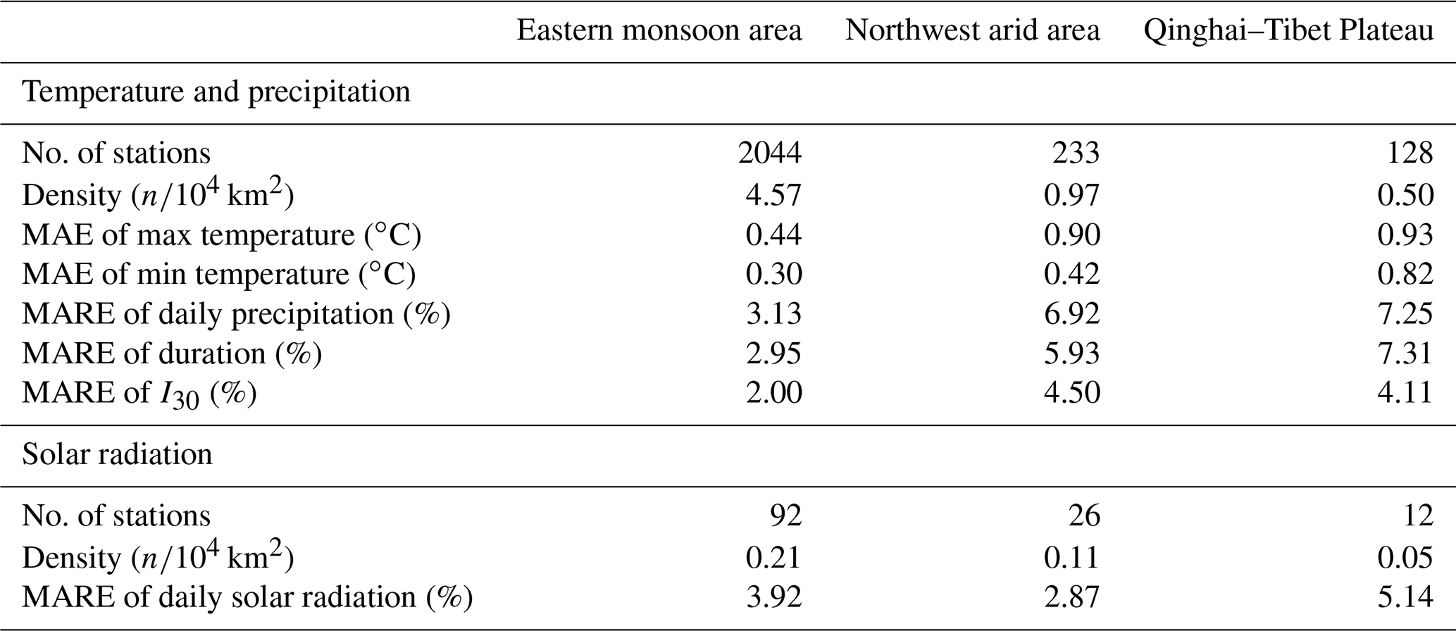
Table 6 Station density and simulation quality of CLIGEN for three Chinese physical-geographical regions.

4 Discussion

Both AE and RE indexes were adopted to evaluate the simulated results in this study. The RE index was applied for solar-radiation- and precipitation-related outputs, while the AE index was applied for the assessment of temperature-related outputs, as RE was not an appropriate indicator to evaluate the temperature which was in interval scale. For stations located in high-latitude or high-altitude areas, the mean annual temperature may be close to zero, resulting in an extremely high RE. For example, the mean maximum temperature of Qian'an station (Fig. 1) using observed inputs was −0.01 ^∘C, and that using interpolated inputs was −0.33 ^∘C, resulting in a RE between the two values of 2912.7 %, which was an extremely large error. However, the mean maximum temperature simulated using the two datasets was very similar, with an AE of 0.32 ^∘C. If RE was used to evaluate the simulated temperature, the actual simulation quality may be strongly underestimated. Therefore, AE values were used to demonstrate errors between generated temperature based on observed and interpolated inputs.

The frequency distributions of CLIGEN-simulated daily precipitation, duration, and peak intensity at Tuokexun station using observed inputs were all not well preserved by those simulated using UK-interpolated inputs (Fig. 8). The simulation quality for Tuokexun was almost the worst among 2405 stations, as RE values for all these three precipitation-related variables were greater than 99 % of stations. This may be explained partially because Tuokexun is located in the northwest arid area of China (Fig. 1), with a station density of 0.97/10⁴ km², which is much lower than that in the eastern monsoon area (Table 6). Stations involved in the interpolation were separated by far distances, with a negative influence on the interpolation accuracy (Oliver and Webster, 2014). Other stations with extremely low simulated quality similar to Tuokexun are almost located in the northwest arid area or the Qinghai–Tibet Plateau, where the station density is lower. The MAE and MARE for generated temperature and precipitation in the eastern monsoon area were the lowest among three physical-geographical regions of China (Table 6). The standard errors of the interpolation results for the two parameters, i.e., TMAX AV and MEAN P, in August are shown as an example (Fig. 9). It can be seen that the errors are relatively high in the western part of China, especially in the northwestern part of the Qinghai–Tibet Plateau, where there is a large area without stations and characterized with the highest standard errors for both parameters (Figs. 1 and 9).

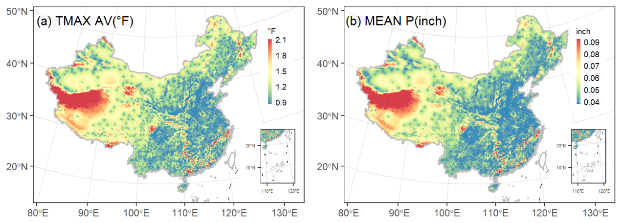
Figure 9 Map of the study area showing the spatial distribution of the standard error for interpolation results of TMAX AV (a) and MEAN P (b) using universal kriging.

The number and density of weather stations for solar radiation were considerably less than for those for temperature and precipitation (Table 6). However, the mean and standard deviation of daily solar radiation using the UK-interpolated parameters was in good agreement with that simulated using observation-based parameter values (Table 4), and MARE of solar radiation was similar to that of daily precipitation. Solar radiation is characterized with much lower spatial variability in comparison to that for the temperature and precipitation. As a result, solar-radiation-related parameters were easier to regionalize, and parameter values could readily be interpolated for regions with limited observations.

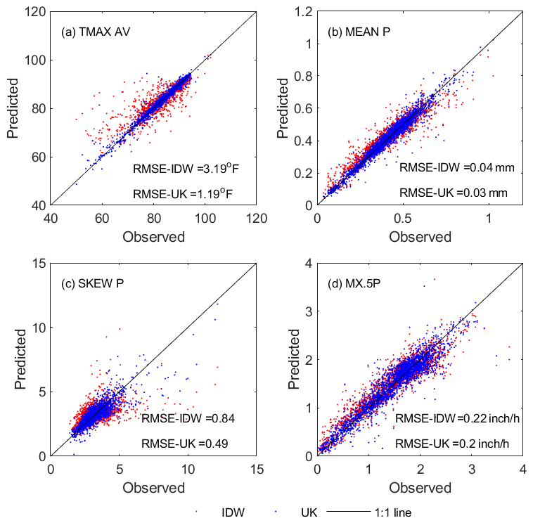
Figure 10 Comparison of interpolation quality using universal kriging (UK) and the inverse distance weighted method (IDW) for CLIGEN temperature- and precipitation-related parameters for 2405 stations in August.

CLIGEN-input parameters in the United States were regionalized from 2600 stations using the inverse distance weighted method (IDW), which was employed in the initial attempt to regionalize CLIGEN input parameters. In this study, UK was adopted to interpolate CLIGEN parameters for mainland China. Interpolated parameter values using IDW and UK were compared for four selected parameters in August as shown in Fig. 10. It can be seen that UK performed better than IDW for all four parameters selected. UK-interpolated parameter values were concentrated mostly along the 1:1 line. The RMSE values of all four groups of parameters interpolated using UK were lower than those predicted using IDW. A noticeable improvement was noted for SKEW P, with the RMSE improving from 0.84 to 0.49 using UK instead of IDW. Therefore, UK appears to be consistently superior to IDW when regionalizing CLIGEN input parameters based on the limited comparison for selected parameters.

5 Code availability

Source code for data extraction, processing, and analysis is available from the authors upon reasonable request.

6 Data availability

The gridded CLIGEN input parameter dataset of China at 10 km resolution is available at the home page of the CLImate Change Impact Assessment (CLICIA) group at http://clicia.bnu.edu.cn/data/cligen.html (last access: 20 May 2021) and https://doi.org/10.12275/bnu.clicia.CLIGEN.CN.gridinput.001 (Wang et al., 2020). Additional materials including the data manual and grid information are also available at the same website and can be downloaded.

7 Summary and conclusion

The widely used stochastic weather generator CLIGEN can simulate long-term climate data to drive hydrological, soil erosion, and crop-yield models. Limitations in high spatial–temporal observations, especially at the sub-daily scale, have partially restricted its application. Daily temperature, daily precipitation, and hourly precipitation data for 2405 stations and daily solar radiation for 130 stations distributed across mainland China were collected to establish the CLIGEN input parameter files and to explore an appropriate method for regionalizing these parameters from stations to the entire region. The predicted quality using two interpolation techniques, OK and UK, was compared and fully assessed, yielding the following results.

1. UK generally performed better than OK when interpolating CLIGEN parameters. Compared with OK, the interpolation accuracy was markedly improved for parameters TMAX AV, TMIN AV, SOL.RAD, MEAN P, SKEW P, P(W|D), and P(W|W). For the remaining parameters, the comparative interpolation accuracies were numerically approximate between the two techniques.

2. UK can accurately predict temperature, solar radiation, and precipitation input parameters for CLIGEN. RMSE values in UK-interpolated parameter values for temperature were less than ≤0.88 ^∘C (1.58 ^∘F),, and NSE for precipitation and solar radiation parameters were all greater than 0.87, except for the skewness coefficient (SKEW P), with a relatively lower interpolation accuracy (NSE = 0.78).

3. Basic statistics and frequency distributions for CLIGEN-simulated climate elements using UK-interpolated parameters agreed well with those simulated using observations. The mean absolute error (MAE) values for the average, standard deviation, and skewness coefficient for the two simulated series of temperature across 2405 stations were all less than 0.5 ^∘C. The mean absolute relative error (MARE) values for same statistics for simulated solar radiation were less than 0.1 %. MARE for the average and standard deviation for precipitation amount, duration, and I₃₀ were less than 5.0 %, while errors for the skewness coefficient for these three groups of parameters were less than 10.1 %.

The developed gridded input parameter database can be applied using CLIGEN, with an established and reliable simulation quality, to the stochastic simulation of temperature, solar radiation, and precipitation at a daily scale and to precipitation at a sub-daily scale for any single point in China. CLIGEN can simulate the dew point and wind as well, which is not regionalized in this study. As a site-based weather generator, simulated climate series using CLIGEN are independent of each other and lack spatial correlations among stations. Further research might focus on the rebuilding of correlations among climate elements and between nearby stations.