the Creative Commons Attribution 4.0 License.
the Creative Commons Attribution 4.0 License.
 | 16 Jun 2021
Year-long, broad-band, microwave backscatter observations of an alpine meadow over the Tibetan Plateau with a ground-based scatterometer
Jan G. Hofste
Rogier van der Velde
Xin Wang
Zuoliang Wang
Donghai Zheng
Christiaan van der Tol
Zhongbo Su
A ground-based scatterometer was installed on an alpine meadow over the Tibetan Plateau to study the soil moisture and temperature dynamics of the top soil layer and air–soil interface during the period August 2017–August 2018. The deployed system measured the amplitude and phase of the ground surface radar return at hourly and half-hourly intervals over 1–10 GHz in the four linear polarization combinations (vv, hh, hv, vh). In this paper we describe the developed scatterometer system, gathered datasets, retrieval method for the backscattering coefficient (σ0), and results of σ0.
The system was installed on a 5 m high tower and designed using only commercially available components: a vector network analyser (VNA), four coaxial cables, and two dual-polarization broad-band gain horn antennas at a fixed position and orientation. We provide a detailed description on how to retrieve the backscattering coefficients for all four linear polarization combinations , where p is the received and q the transmitted polarization (v or h), for this specific scatterometer design. To account for the particular effects caused by wide antenna radiation patterns (G) at lower frequencies, σ0 was calculated using the narrow-beam approximation combined with a mapping of the function over the ground surface. (R is the distance between antennas and the infinitesimal patches of ground surface.) This approach allowed for a proper derivation of footprint positions and areas, as well as incidence angle ranges. The frequency averaging technique was used to reduce the effects of fading on the uncertainty. Absolute calibration of the scatterometer was achieved with measurements of a rectangular metal plate and rotated dihedral metal reflectors as reference targets.
In the retrieved time series of for L-band (1.5–1.75 GHz), S-band (2.5–3.0 GHz), C-band (4.5–5.0 GHz), and X-band (9.0–10.0 GHz), we observed characteristic changes or features that can be attributed to seasonal or diurnal changes in the soil: for example a fully frozen top soil, diurnal freeze–thaw changes in the top soil, emerging vegetation in spring, and drying of soil. Our preliminary analysis of the collected time-series dataset demonstrates that it contains valuable information on water and energy exchange directly below the air–soil interface – information which is difficult to quantify, at that particular position, with in situ measurement techniques alone.
Availability of backscattering data for multiple frequency bands (raw radar return and retrieved ) allows for studying scattering effects at different depths within the soil and vegetation canopy during the spring and summer periods. Hence further investigation of this scatterometer dataset provides an opportunity to gain new insights in hydrometeorological processes, such as freezing and thawing, and how these can be monitored with multi-frequency scatterometer observations. The dataset is available via https://doi.org/10.17026/dans-zfb-qegy (Hofste et al., 2021). Software code for processing the data and retrieving via the method presented in this paper can be found under https://doi.org/10.17026/dans-xyf-fmkk (Hofste, 2021).
- Article
(14003 KB) - Full-text XML
- BibTeX
- EndNote


To comprehend the climate of the Tibetan Plateau, also known as the “Third Pole Environment”, the transfer processes of energy and water at the land–atmosphere interface must be understood (Seneviratne et al., 2010; Su et al., 2013). Main states of interest are the dynamics of soil moisture and temperature (Zheng et al., 2017a). Together with sensors embedded into the deeper soil layers, microwave remote sensing is suitable to study these dynamics since it directly probes the top soil layer within the antenna footprint.
A ground-based microwave observatory was installed on an alpine meadow over the Tibetan Plateau, near the town of Maqu. The observatory consists of a microwave radiometer system called ELBARA-III (ETH L-Band radiometer for soil moisture research) (Schwank et al., 2010; Zheng et al., 2017b) and an microwave scatterometer. Both continuously measure the surface's microwave signatures with a temporal frequency of once every hour. The ELBARA-III was installed in January 2016 and is currently still measuring (Zheng et al., 2019; Su et al., 2020); the scatterometer was installed in August 2017 and continued to operate until July 2019.
This paper describes the scatterometer system and the collected dataset over the period August 2017–August 2018 (Hofste et al., 2021). The radar return amplitude and phase were measured over a broad 1–10 GHz frequency band at all four linear polarization combinations (vv, hv, vh, hh). The scatterometer measured the radar return over a prolonged period with its antennas in a fixed orientation, resulting in frequency-dependent incidence angle ranges varying from of for L-band (1.625 GHz) to for X-band (9.5 GHz). During the summers of 2017 and 2018 additional experiments were conducted to assess the angular dependence of the backscatter and homogeneity of the local ground surface.
Many other studies exist employing ground-based systems to study microwave backscatter from land. Rather than an airborne or spaceborne system, ground-based systems allow for high temporal coverage and a high degree of control over the experimental circumstances. Geldsetzer et al. (2007) and Nandan et al. (2016) used specially developed radar systems by ProSensing Inc. to study backscattering from sea ice in the period 2004–2011: one system for C-band and another for X- and Ku-band. Details on a similar S-band system can be found in Baldi (2014). The SnowScat system, developed by Gamma Remote Sensing AG (Werner et al., 2010), is another scatterometer that operates over 9–18 GHz and measures the full polarimetric backscatter autonomously over many elevation and azimuth angles. Lin et al. (2016) used it during multiple winter campaigns in the 2009–2012 period at two different locations to study the scattering properties of snow layers. Like in this study, others also designed their scatterometer architecture around a commercially available vector network analyser (VNA). For instance, Joseph et al. (2010) used data measured by a truck-based system, operating at C- and L-band, in summer 2002 to study the influence of corn on the retrieval of soil moisture from microwave backscattering. For every band they placed one antenna to transmit and receive on top of a boom. Selection of the individual polarization channels was realized using radio-frequency switches. Similar is the University of Florida L-band Automated Radar System (UF-LARS) (Nagarajan et al., 2014), used by for example Liu et al. (2016), to measure soil moisture at L-band from a Genie platform during summer 2012. Another example is the Hongik Polarimetric Scatterometer (HPS) (Hwang et al., 2011), with which microwave backscatter from bean and corn fields was measured in 2010 and 2013 respectively (Kweon and Oh, 2015). Similar to our study, Kim et al. (2014) used a scatterometer with its antenna in a fixed position and orientation to measure the backscattering during all growth stages of winter wheat at L-, C-, and X-band during 2011–2012.
The temporal resolution and measurement period covered by the scatterometer dataset reported in this paper permits studying both seasonal and diurnal dynamics of microwave backscattering from an alpine meadow ecosystem. This in turn allows for investigating the local soil moisture dynamics, the freeze–thaw process, and growth/decay stages of vegetation. Because of the broad frequency range measured (1–10 GHz), wavelength-dependent effects of surface roughness and vegetation scattering can be studied as well.
This paper is organized as follows. First the study area is described. Next, details are provided on the instrumentation used, measurements performed, and method for retrieving the backscattering coefficient σ0 (m2 m−2). We then present an overview of the retrieved σ0 time-series dataset and show how σ0 varies across seasons and on a diurnal timescale. In the discussion section the angular and spatial variability of σ0 at the study area and measurement uncertainty are described. Technical details on all aspects of the scatterometer measurements and σ0 calculation are included in the Appendix. A list of symbols can be found at the end of this paper.
In August 2017 the scatterometer was installed on the tower of the Maqu measurement site (Maqu site) (Zheng et al., 2017b) and operated over the period August 2017–June 2019. The Maqu site is situated in an alpine meadow ecosystem (Miller, 2005) on the Tibetan Plateau, Fig. 1a. The site's coordinates are 33∘55′ N, 102∘10′ E, at 3500 m elevation. The site is located close to the town Maqu of the Gansu province of China.

Figure 1(a) Location of Maqu measurement site on eastern part of the Tibetan Plateau. (b) Tower of Maqu site containing the scatterometer, the ELBARA-III radiometer, and Piccolo optical spectroradiometer.
Besides the scatterometer, other remote sensing sensors placed on the tower are the ELBARA-III radiometer (Schwank et al., 2010) and the optical spectroradiometer system Piccolo (MacArthur et al., 2014), Fig.1b. The ELBARA-III system has been measuring L-band microwave emission since January 2016 to this date (Zheng et al., 2019; Su et al., 2020). The Piccolo system measured the reflectance and sun-induced chlorophyll fluorescence of the vegetation over the period July–November 2018.
According to Peel et al. (2007) the climate at Maqu is characterized by the Köppen–Geiger classification as “Dwb”: cold with dry winters. Winter (December–February) and spring (March–May) are cold and dry, while the summer (June–August) and autumn (August–November) are mild with monsoon rain.
The ecosystem classification of the Maqu site is “alpine meadow” according to Miller (2005). The vegetation around the Maqu site consists of grasses for the most part. The growing season starts at the end of April and ends in October, when above-ground biomass turns brown and loses its water. During the growing season the meadows are regularly grazed by livestock. To prevent the livestock from entering the site and damaging the equipment, a fence is placed around the Maqu site. As a result there is no grazing within the site, causing the vegetation to be more dense and higher than that of the surroundings. Also a layer of dead plant material from the previous year remains present below the newly emerged vegetation. In Appendix Sect. A1 some photographs are shown of the Maqu site during different seasons, which provide an impression of the site's phenology.
3.1 Supporting measurements
Together with the scatterometer, measurements following hydrometeorological quantities were recorded over the period August 2017–August 2018: depth profile of volumetric soil moisture mv (m3 m−3) and soil temperature Tsoil (∘C), air temperature Tair (∘C), precipitation (mm), and the short- and long-wave up- and downward irradiance (W m−2). Details on used sensors can be found in Appendix Sect. A2.

Figure 2Map of the Maqu site. Scatterometer footprints for C-band with vv polarization are shown for different α0 (40, 55, 70∘) and ϕ (−30, −20, …, 30∘) angles. For time-series measurement antennas were fixed at and .
The depth profile of mv (m3 m−3) was measured with an array of 20 capacitance sensors, type 5TM (manufacturer: Meter Group), that were installed at depths ranging from 2.5 cm to 1 m (Lv et al., 2018). All sensors in the array are also equipped with a thermistor, enabling the measurement of Tsoil (∘C). The soil moisture and temperature was logged every 15 min for the period of August 2017–August 2018 with Em50 data loggers (manufacturer: Meter Group) that were buried near the sensors. The location of the buried sensor array is indicated in Fig. 2. Results of these hydrometeorological measurements over the period August 2017–August 2018 can be found in Appendix Sect. A2 as well. With a handheld impedance probe, type ThetaProbe ML2x (manufacturer: Delta-T Devices), the spatial variability of mv in the top 2.5–5 cm soil layer over the Maqu site was measured (Appendix Sect. A3).
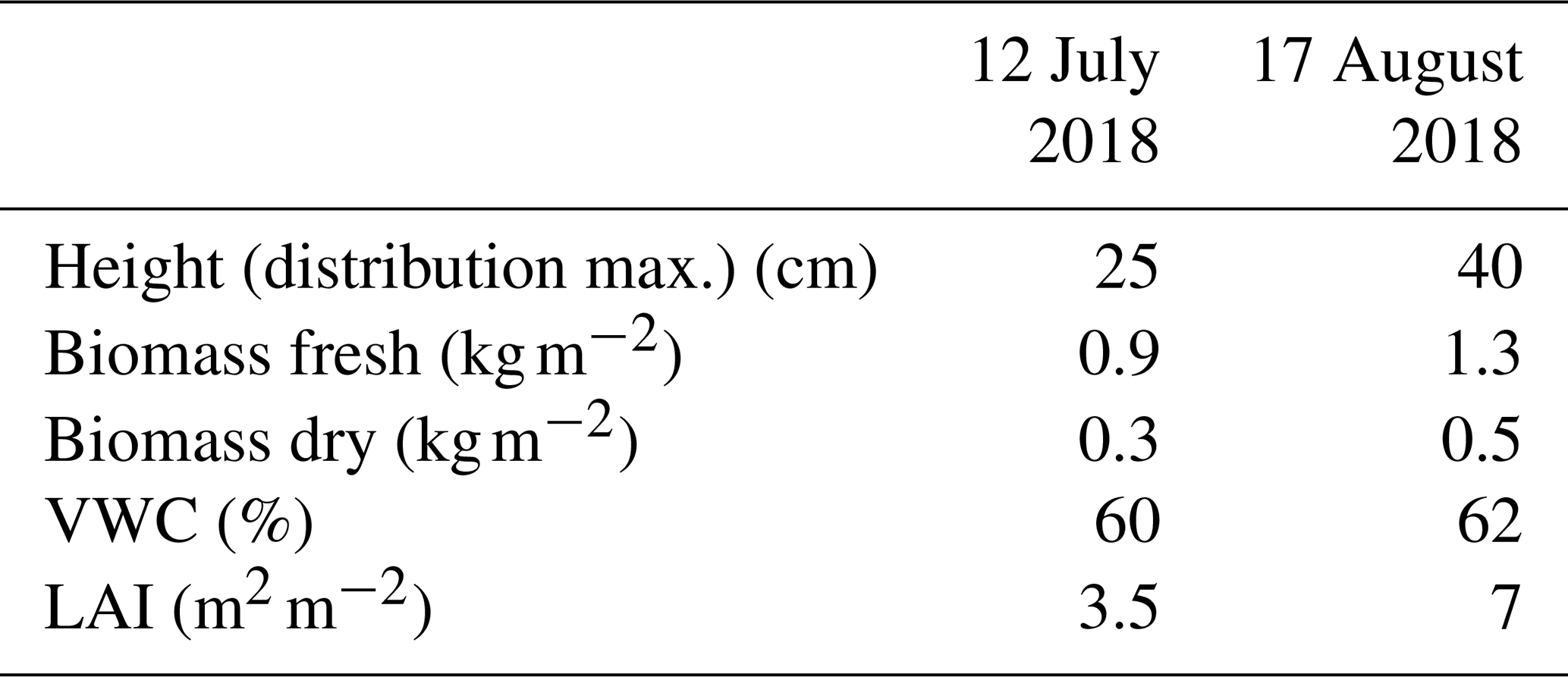
To quantify the vegetation cover at the Maqu site, measurements were performed on 2 d during the 2018 summer, namely 12 July and 17 August. Vegetation height, above-ground biomass (fresh and oven-dried), and leaf area index (LAI) (m2 m−2) were measured at ten 1.2×1.2 m2 sites around the periphery of the “no-step zone” indicated in Fig. 2. The vegetation height of a single site was determined as the maximum value of the histogram obtained by taking ≥30 readings with a thin ruler at random points within the site area. For each site, above-ground biomass and LAI were determined from harvested vegetation within one or two disk areas defined by a 45 cm diameter ring. Immediately after harvest all biomass was placed in airtight bags so that the fresh and dry biomass could be determined by weighing the bag's content before and after drying in an oven. The LAI was determined immediately after harvest with part of the harvested fresh biomass by the method described in He et al. (2007). The obtained average quantities over the 10 sites are summarized in Appendix Sect. A4.
3.2 Scatterometer
3.2.1 Instrumentation
The main components of the scatterometer are a two-port vector network analyser (VNA), type PNA-L 5232A (manufacturer: Keysight); four 3 m long phase-stable coax cables, type Sucoflex SF104PEA (manufacturer: Huber + Suhner); and two dual-polarized broad-band horn antennas, type BBHX9120LF (manufacturer: Schwarzbeck); see Fig. B1. The antenna radiation patterns are measured in the principal planes by the manufacturer over the 1–10 GHz band (Schwarzbeck Mess-Elektronic OHG, 2017). As a summary, the full width at half maximum (FWHM) intensity beamwidths over frequency are shown in Fig. B3. To protect the VNA from weather it is placed inside a waterproof enclosure equipped with fans to provide air ventilation.
Deployed reference targets to calibrate the scatterometer were a rectangular plate and two dihedral reflectors. The rectangular plate reflector was constructed from lightweight foam board covered with 100 µm aluminium foil and had frontal dimensions a=85 cm × b=65 cm. A small dihedral reflector was constructed from steel, and its frontal dimensions were a=57 cm × b=38 cm. A second large dihedral reflector was also constructed with foam board and aluminium foil, and its frontal dimensions were a=120 cm × b=65 cm. A height-adjustable metal mast was used to position the reference targets. To minimize reflection from this mast, it was covered by pyramidal absorbers, type 3640-300 (manufacturer: Holland Shielding), having a 35 dB reflection loss for normal incidence at 1 GHz.
3.2.2 Experimental setup and procedures
The scatterometer is placed on a tower as shown in Fig. 1b. The two antenna apertures are at a distance approximately Hant=5 m above the ground (Hant depends on the antenna boresight angle α0) and are separated from each other horizontally by Want=0.4 m. The connection scheme of the VNA and the two antennas is described in Appendix Sect. B1. In Appendix Sect. B2 further details on the setup geometries can be found. During all experiments, VNA measurements were performed with a stepped 0.75–10.25 GHz frequency sweep at 3 MHz resolution (3201 points). The dwell time per measured frequency was 1 µs, which is equivalent to a two-way travelling distance for the microwave signal of 150 m. The intermediate-frequency (IF) bandwidth was minimized to 1 KHz to increase the signal-to-noise ratio.
The radar return from the rectangular metal plate reference target was used to calibrate the scatterometer for the co-polarization channels. The two metal dihedral reflectors were used as depolarizing reference targets (Nesti and Hohmann, 1990) to calibrate the cross-polarization channels. We used two dihedrals, measured at different distances R0 (m), in order to meet requirements concerning target size, target distance (plane wave criteria), and ground-to-target interference removal. Readers are referred to Appendix Sect. B3 for the measurement details and validation-exercise results.
Time-domain filtering, or gating, was used as part of post-processing to remove the antenna-to-antenna coupling and undesired scattering contributions from the radar return signal for both the reference target and the ground return measurements. The application of gating with VNA-based scatterometers is described in more detail in for example Jersak et al. (1992) or De Porrata-Dória i Yagüe et al. (1998). Details on our gating process and related peculiarities regarding our scatterometer can be found in Appendix Sect. B4.
Table 1Overview of performed scatterometer experiments and their respective α0 and ϕ ranges. Antennae aperture height Hant depends on α0.
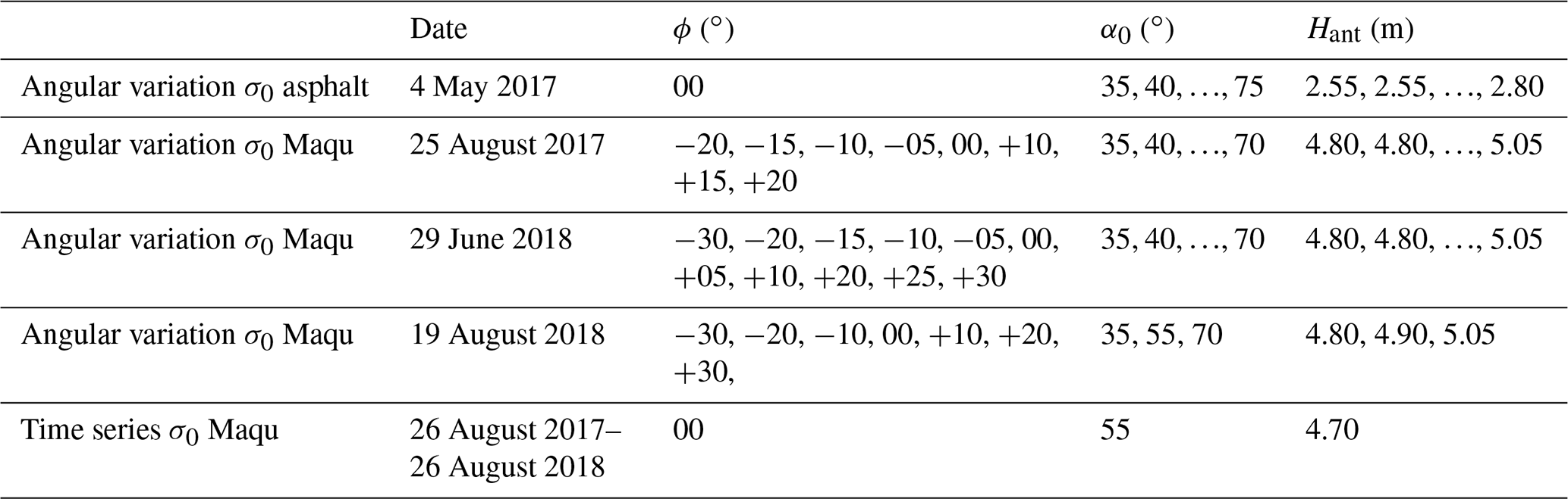
In this paper, we focus on the time-series measurements of σ0 over a 1-year period, during which measurements were taken either once or twice per hour. With this experiment, the antennas were fixed on a tower rod, such that the angle between the antenna boresight line and the ground surface normal α0 was 55∘ and the azimuth angle ϕ was fixed at 0∘ as shown in Fig. 2. Although varying the antennae orientations (using automatic motorized rotational stages) to measure backscatter under various incidence and azimuth angles would be preferable from an experimental perspective, this approach was abandoned because it would make the setup extra vulnerable to system failures. Measurements of σ0 for different α0 and ϕ angles at the Maqu site were, however, performed during 3 separate days. These measurements are discussed in Sect. 5.3. Before installing the scatterometer at the Maqu site, exploratory experiments were performed in which σ0 over α0 was measured for asphalt and subsequently compared to results in other studies (Sect. 5.1). Table 1 summarizes all experiment geometries and dates of execution. For the angular-variation experiments the scatterometer antennas were mounted on a motorized rotational stage. Depending on the angle α0, Hant would vary according to , with H0=2.95 or 5.2 m for the asphalt or Maqu experiments respectively. All angular-variation experiments were conducted within one afternoon.
3.2.3 σ0 retrieval procedure
The power received by a monostatic radar or scatterometer system from a distributed target with backscattering coefficient (m2 m−2) is given by the radar equation (Ulaby et al., 1982)
where it is assumed that the same antenna is used for both transmitting (TX) and receiving (RX). is the transmitted and the received power respectively (W). The subscripts of the powers refer to the linear polarization directions: horizontal (h) or vertical (v). With the first subscript refers to the polarization direction of the scattered and the second to that of the incident wave. G (–) denotes the normalized angular gain pattern of the antenna with peak value G0 (–). Equation (1) represents an ideal lossless system – in practice any scatterometer has frequency-dependent losses or other signal distortions. These frequency-dependent phase and amplitude modulations can be accounted for by measuring the radar return of a reference target with known radar cross section (RCS) σpq (m2) (Eq. B2) to calibrate the system. This procedure, often referred to as external calibration, is mathematically represented by
where R0 (m) is the distance at which the reference target was measured. In the case of a scatterometer with narrow beamwidth antenna, all integrand terms of Eq. (2) can be approximated as being constants, the so-called “narrow-beam approximation” (Wang and Gogineni, 1991), so that we obtain
where Afp is the scatterometers “footprint”, notably the area (m2) for which the surface projected antenna beam intensity is equal to or larger than half its maximum value. Rfp (m) refers to the distance between the antenna and footprint centre.
For this dataset is estimated by employing Eq. (3) in combination with a mapping of the term from Eq. (2) over the ground surface. Due to the wide antenna radiation patterns, especially with low frequencies, the area that is to be associated with the measured scatterometer signal, i.e. the footprint, is typically not located where the antenna boresight line intersects the ground surface. Instead the footprint appears closer to the tower base. Figure 3 demonstrates this effect for the case of 5 GHz at α0=55∘, by showing the mapping of over the ground surface. This footprint-shift effect is strongest with the widest antenna radiation patterns (thus with low frequencies) and for large α0 angles. The footprint position and dimensions were found using the mapping over the ground surface. The applied criterion was that the footprint contains 50 % of the total projected intensity onto the ground surface. After the footprint edges were defined the incidence angle ranges were derived from them using trigonometry.
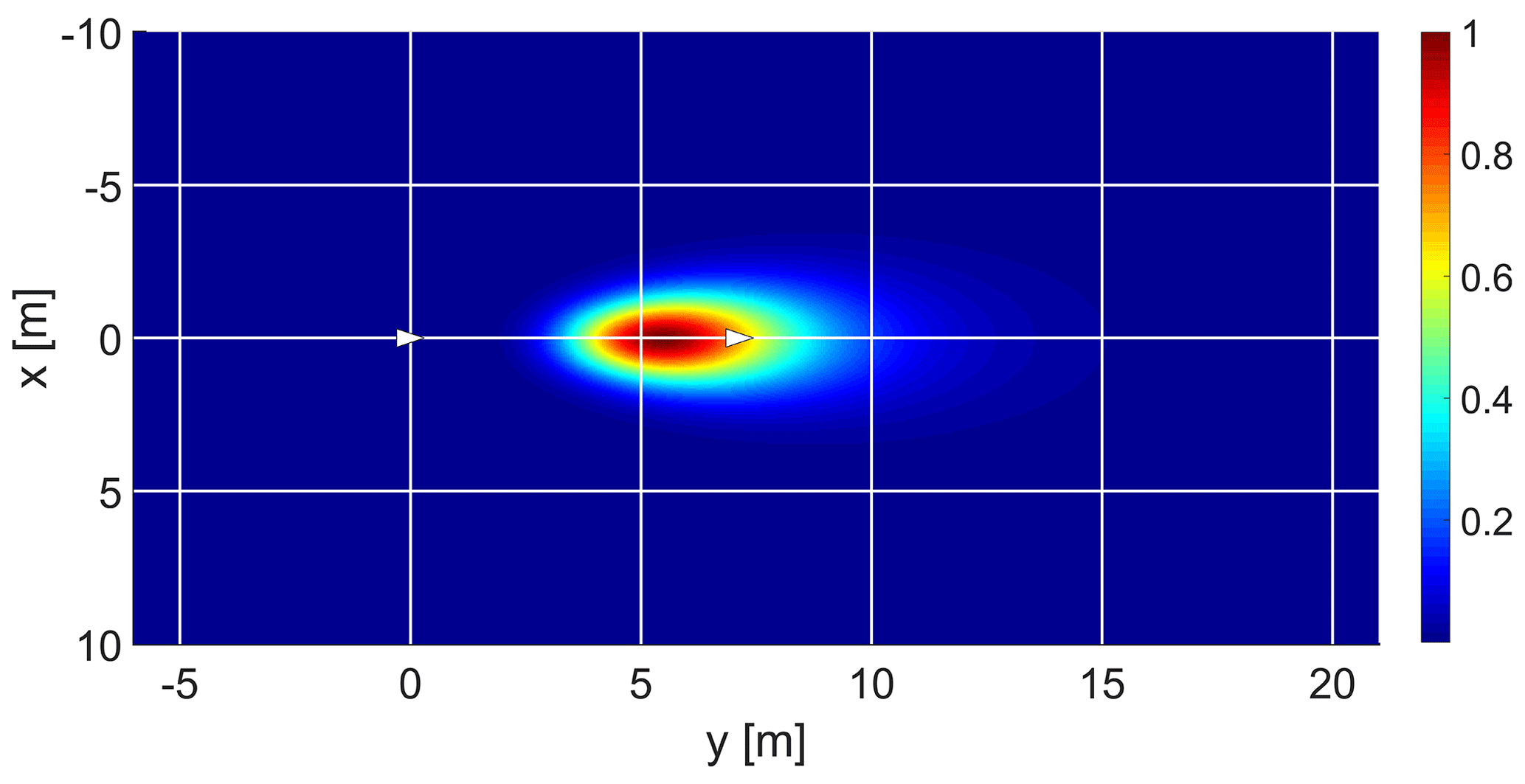
Figure 3Example of with Gaussian antenna radiation patterns. Plot normalized to its peak value. x and y are ground surface coordinates. The white triangle at coordinate (0,0) represents the tower location and the other white triangle indicates the intersection point of the antenna boresight line and the ground surface. , f=5 GHz and polarization is vv.
Because of the low directivity (gain) of the antennas and unknown nature of over θ, there is an inherent uncertainty in our retrieved values (for a certain θ range). This matter is discussed further in Sect. 5.2.
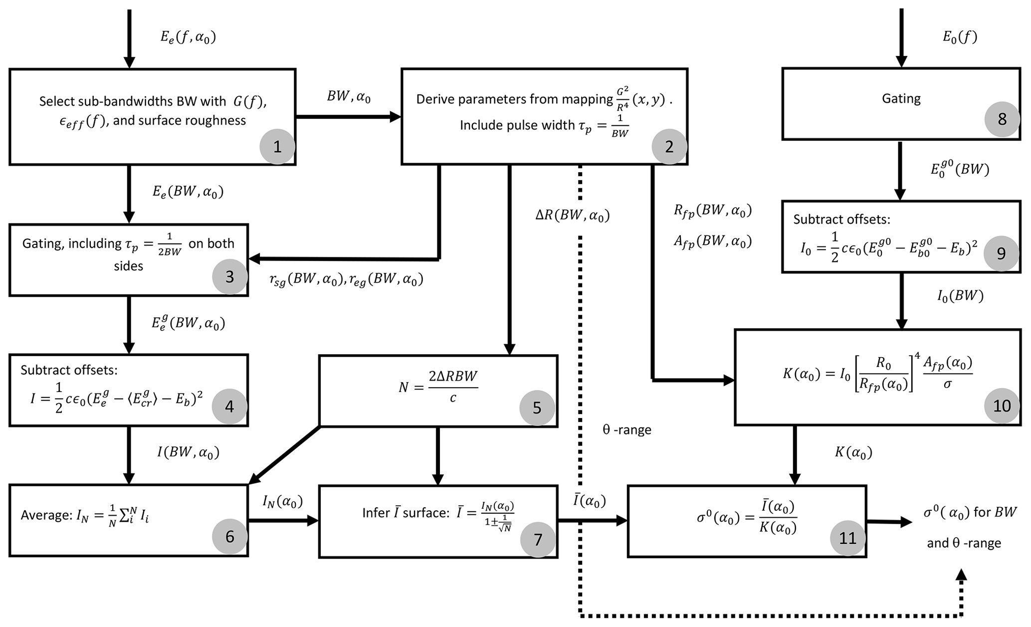
Figure 4Flow chart of σ0 derivation process. Inputs are the measured backscattered electric fields of the surface target Ee(f,α0) and the calibration standard E0(f). The process follows from 1 to 11 in sequence.
In Fig. 4 the procedure for deriving the backscattering coefficient is depicted. The equations used therein are derived from Eq. (3). Refer to Appendix Sect. C1 for more information. The different steps indicated in the figure are explained here.
-
We start with Ee (V m−1), the measured backscattered electric field from the ground target incident on the receiving antenna. The subscript e denotes “envelope” magnitude of the complex signal, as in Ulaby et al. (1988)1. This quantity is measured over the full 0.75–10.25 GHz band at angle α0: Ee(f,α0). Bandwidths (BW) are selected based on the change in G(α,β) over frequency (Appendix Sect. B4), the number of independent frequency samples N that may be retrieved from BW, and the estimated change in backscattering properties over frequency of the ground surface as is discussed in Appendix Sect. C2. Result is the bandwidth selection Ee(BW,α0).
-
With BW and α0 as input, is mapped for all frequencies within BW using the antenna radiation patterns measured by the manufacturer. The region associated with 50 % of the total projected intensity onto the ground is determined to set appropriate gating times, or distances rsg and reg (m), and for calculating the Afp, Rfp, and the θ range. Half the pulse width is subtracted from rsg and added to reg, and quantities Afp, Rfp, and the θ range are changed accordingly.
-
The gate is applied to Ee(BW,α0), resulting in the gated backscattered field , where the superscript g indicates that the signal is gated.
-
The bandwidth-average coupling remnant (V m−1) and minimal detectable signal Eb (V m−1) are subtracted from for each measured frequency. is an offset formed by part of the signal transmitted from the transmit antenna coupling directly into the receive antenna (antenna cross coupling). Although the majority of this coupling can be filtered out by using time-domain gate filtering, a remnant is still present (hence “coupling remnant” in the subscript) and must be accounted for (Appendix Sect. E4). Note that the same gate as with is applied. A similar form of offset subtraction from was done in for example Nagarajan et al. (2014). Next, the result is squared and converted into intensity I(BW,α0) (W m−2).
-
To reduce the radiometric uncertainty due to fading we perform frequency averaging. The number of statistically independent frequency samples N within BW is calculated with (m). Please refer to Appendix Sect. C2 for more information.
-
From the I(BW,α0) spectrum N intensities are selected at equidistant intervals of (Hz) and averaged to IN(α0).
-
With IN(α0) and N, the average received intensity (W m−2) is calculated using Eq. (C4). The denominator implies that is estimated with a 68 % confidence interval.
-
The gated backscattered signal from the reference target (V m−1) (subscript 0 represents “reference”; superscript g0 stands for “gate” during reference measurements) is determined for the full 0.75–10.25 GHz band under the assumption that G≈1 for all frequencies (see Appendix Sect. B4). After gating the relevant BW of is selected.
-
The measured response from the mast without reference target (V m−1) is subtracted from the reference target response. Subscript b0 denotes background calibration, and the superscript g0 indicates that the same gate was used as with the reference target response. Also Eb is subtracted here. The result is squared and converted into intensity I0(BW) (W m−2).
-
The I0(BW) is used to calculate the factor K (W m−2), given the footprint area Afp and centre distance Rfp (Eq. C2).
-
The final step is the application of Eq. (C1) with and K(α0) as inputs to obtain σ0. By steps 2 and 6 the derived σ0 is to be associated with the chosen BW and calculated θ range. By step 7 a 68 % confidence interval applies to σ0.
For the analyses in this paper we discuss results of four bandwidths BW, picked amidst frequency ranges typically used in microwave remote sensing: 9–10 GHz (X-band), 4.5–5 GHz (C-band), 2.5–3 GHz (S-band), and 1.5–1.75 GHz (L-band). The widths decrease with wavelength due to the expected frequency resolution of the target's scattering response (Appendix Sect. C2) and the antenna-radiation-pattern change over frequency (Appendix Sect. B4). Presented in this section is, first, a global overview of the retrieved over the period 26 August 2017–26 August 2018, followed by a 13 d time series of at the highest temporal resolution during the thawing period in April 2018.
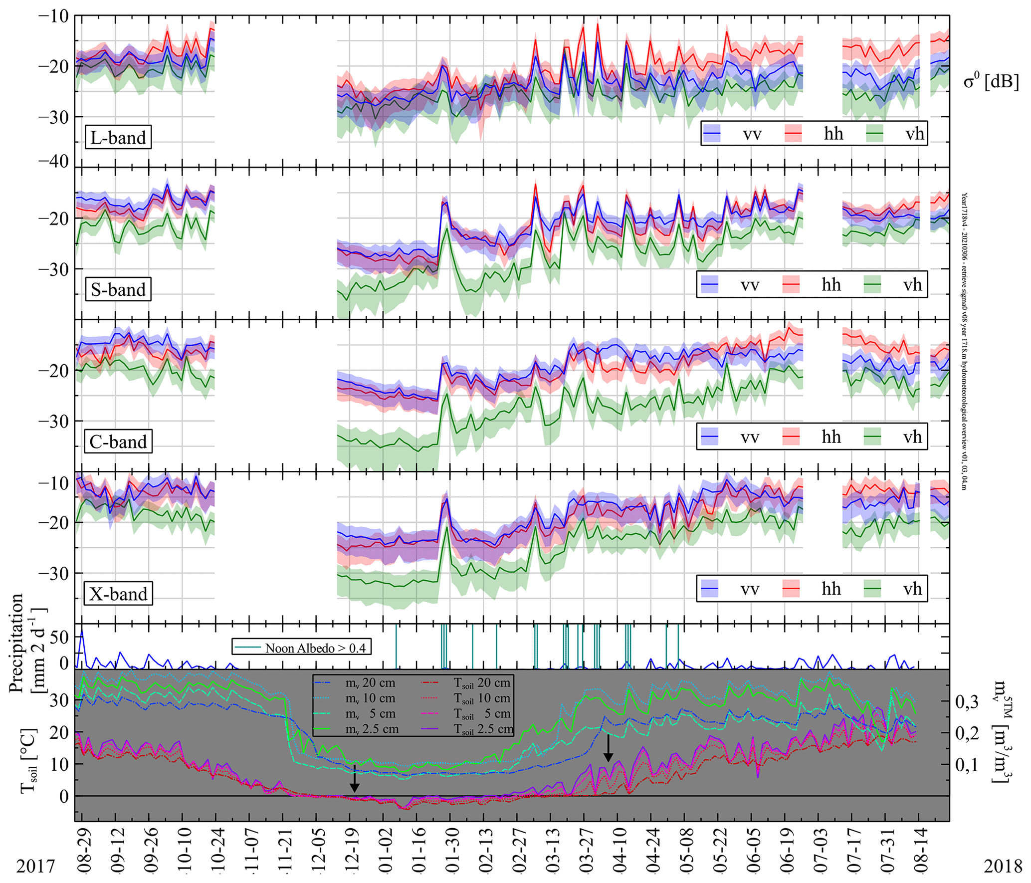
Figure 5Time-series measurements of (m2 m−2) for L-, S-, C-, and X-band, Mv, and Tsoil from August 2017 to 2018. Shown are measurements taken at 18:10 LT with 2 d intervals. Shaded regions indicate 66 % confidence intervals for . The antenna boresight angle was fixed at . The incidence angle ranges were band and polarization dependent. The widest ranges were for L-band, for S-band, for C-band, and for X-band. Bottom graphs show measured precipitation per 2 d (snowfall identified by noon albedo), volumetric soil moisture (m3 m−3), and soil temperature Tsoil at indicated depths. Arrows indicate frozen/thawed soil at 25 cm. Spatial average volumetric soil moisture Mv is estimated as m3 m−3.
Figure 5 presents an overview of the time-series data of over the whole August 2017–2018 period for all considered bandwidths in L-, S-, C-, and X-band, along with Mv and Tsoil at four depths ranging from 2.5 to 20 cm and precipitation. Based on observed albedo values, days at which a layer of snow was present are indicated. For visibility reasons the graphs only display measurements taken at 18:10 LT with 2 d intervals and one cross-polarization channel ( and are within each other's confidence intervals). Data of the radar return and for November 2017 are not available, while those of late June–Early July 2018 will become available at a later stage.
We observe for all bands and polarizations that σ0 is highest in summer and autumn, while it is lowest during winter. The same observations were made with satellites over the Maqu area for L-band (Wang et al., 2016) and C-band (Dente et al., 2014). This behaviour can be explained by the fact that in summer and autumn Mv and the amount of fresh biomass is highest. As a result, the high dielectric constant of moist soil in combination with the rough surface and presence of water in the vegetation results in strong backscattering. During winter, however, there is little liquid water, i.e. Mv, present in the soil and no fresh biomass (dry biomass however remains present; see Fig. A1). Black arrows indicate frozen and thawed soil at 25 cm depth (Appendix Sect. A2). The dielectric constant of the soil therefore is lower compared to that of moist soil, and there is little to no scattering from the dried out vegetation, resulting in a lower . All aforementioned effects are described in, for example, (Ulaby and Long, 2017). There were, however, also peaks of during winter, for example on 26 January, which coincided with snowfall. In (Lin et al., 2016) strong backscatter increments due to fresh snowfall were also observed for X-band. Apparently, this behaviour is similar with the longer wavelengths as the graphs show.
When comparing the four bands we observe that, in general, the backscattering is highest for X-band and lowest for L-band or S-band. This difference is mainly driven by the wavelength-dependent response to the surface roughness of the soil and vegetation during the summer and autumn period. For longer wavelengths the soil surface roughness appears smoother than for the shorter wavelengths, resulting in stronger specular reflection, thus lower backscatter. A similar argument holds for the vegetation: its constituents are small compared to the longer wavelengths; thus little volume scattering occurs.
Except for during the summer, backscatter for vv polarization was equal to or higher than that for hh polarization. This behaviour was also observed by Oh et al. (1992), albeit for bare soil. We, however, may compare our situation to that of bare soil during winter, when there is no fresh biomass. When vegetation was present, was stronger for all bands, as is visible during June–August 2018. This was however not the case during August–September 2017, when the vegetation probably still contained water. Somewhat stronger backscatter, 0.5–1 dB, for hh than for vv polarization was also reported for grassland in Ulaby and Dobson (1989) with for S- and X-band. For C-band they reported no clear difference. Yet another study, (Kim et al., 2014), measured 3–4 dB higher backscatter for hh than for vv polarization when measuring wheat at L-band (). Our results for L-band were similar. Cross-polarization σ0 levels were, as expected, lower than those of co-polarization. During the winter period this difference was largest, especially with C-band. For L-band, on the other hand, this difference in σ0 levels between co-polarization and cross polarization was quite small.
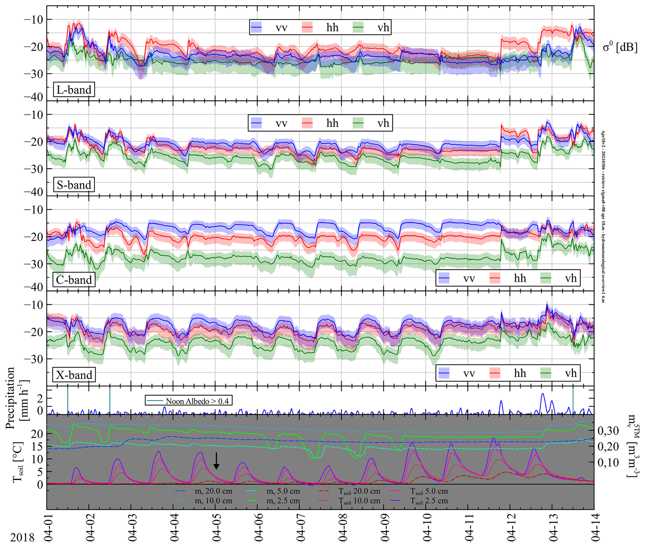
Figure 6Time-series measurements of (m2 m−2) for L-, S-, C-, and X-band, precipitation, Mv, and Tsoil during 13 d in April 2018. Shaded regions indicate 66 % confidence intervals for . The antenna boresight angle was fixed at . The incidence angle ranges were band and polarization dependent. The widest ranges were for L-band, for S-band, for C-band, and for X-band. Bottom graphs show measured precipitation (mm h−1) (snowfall identified by noon albedo), volumetric soil moisture (m3 m−3), and soil temperature Tsoil at indicated depths. Arrow indicates thawing of soil at 25 cm. Spatial average volumetric soil moisture content Mv is estimated as m3 m−3.
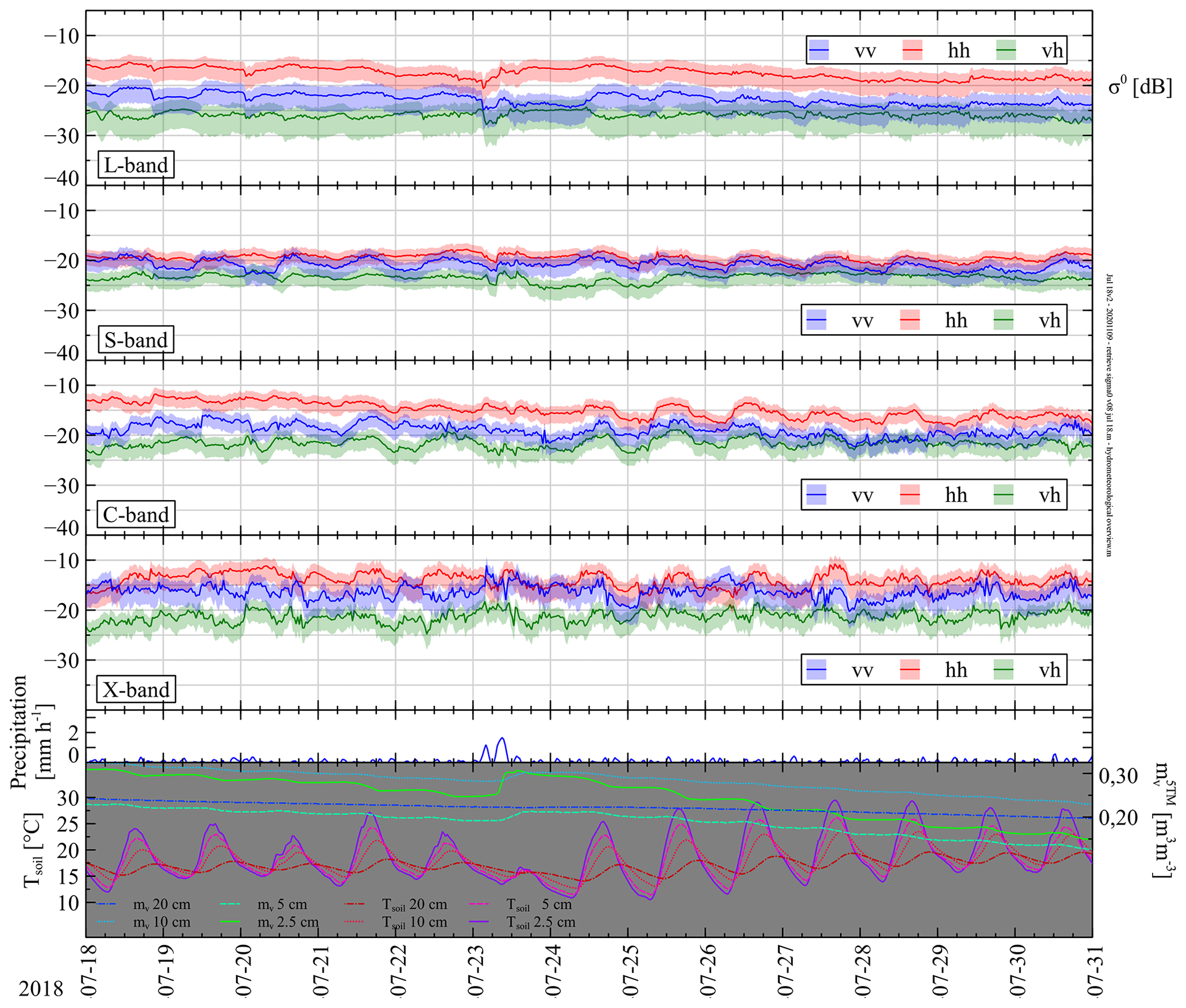
Next, four 13 d time series of σ0 at 30 min intervals are presented. When selecting these periods we tried avoiding strong precipitation events as much as possible, since these complicate the interpretation. In Appendix Sect. D time series during October 2017 (Fig. D1), December 2017 (Fig. D2), and July 2018 (Fig. D3) can be found. Here we shall describe the retrieved during a 13 d period in April 2018 (Fig. 6) when the thawing process was ongoing.
The most prominent features in Fig. 6 are the diurnal variations of that are clearly caused by changes in Mv. For S-, C-, and X-bands we observe that σ0 increases during daytime due to the increase in liquid water in the top soil due to thawing, and at night σ0 drops as most of the water freezes again. For L-band this behaviour is also visible, though not as pronounced. The Mv changes at different depths are consistent with this difference: the strongest diurnal variation in liquid water was measured by the probes at 2.5 and 5 cm depth, while those at 10 and 20 cm do not change as much. On some days, for example on 4 and 5 April, or on 10 April, we observe diurnal changes in σ0 (most pronounced for X-band), while the Mv measured by the 5TM sensors at 2.5 and 5 cm depth showed little variation. This may suggest that the freezing and thawing during those days occurred only in the very top soil layer, just below the air–soil interface where it was outside the influence zone of the 5TM sensors. The time lag between the drop of σ0 (first) and the drop of 5TM Mv (second) is caused by the same phenomena as the freezing starts at the top soil layer and progresses downward. The time lag during thawing was smaller. In general the magnitude of the σ0 change was largest for X-band and smallest for L-band, though exceptions exist. See for example 3 April, where for L-band drops almost 10 dB, which is more than for other bands. At the same time Mv at 20 cm depth also shows strong variation, while Mv at 10 cm changes less.
5.1 Reference measurements for asphalt
In order to check our scatterometer setup and σ0 retrieval procedure an experiment was performed in which the backscatter of asphalt was measured and subsequently compared to results found in other studies. This exercise is described in Appendix Sect. F. We found that our results for X-band with co-polarization and S-band for vv and vh polarization match with those reported in Ulaby and Dobson (1989) and Baldi (2014) respectively. For L-band a proper comparison was not possible due to the width of our antenna patterns. We could not find other studies reporting backscatter for C-band to compare our results to.
5.2 Measurement uncertainty
In the derivation of σ0 we distinguish four sources of uncertainty: (i) fading (Sect. 3.2.3), (ii) the temperature-induced radar return uncertainty ΔET (V m−1), (iii) reference target measurement uncertainty ΔK (in dB, as it is a relative value), and (iv) the low-directivity-induced uncertainty.
First we describe (ii) and (iii), which are systematic sources of uncertainty. In this context we also consider the system's offsets levels formed by the antenna-to-antenna coupling remnant (V m−1) and the minimum signal strength measurable by the VNA, or background Eb (V m−1). The former is derived from measurements with the antennas aimed skywards. From Eb the minimum measurable RCS (given a certain distance R to target) σmin can be calculated via Eq. (3), where instead of the product σ0Afp a RCS value is to be calculated using the power levels associated with Eb. Appendix Sect. E contains detailed information on all considered systematic sources of uncertainty and offsets, starting with an overview (Appendix Sect. E1), followed by sections on ΔET (Appendix Sect. E2), ΔK (Appendix Sect. E3), and (Appendix Sect. E4).
Starting with Eq. (C1) it can be shown (see Appendix Sect. E5) that the three estimated types of uncertainty, namely fading, temperature-induced radar return uncertainty (ΔET), and reference target measurement uncertainty (ΔK), can be combined in a model for total σ0 uncertainty:
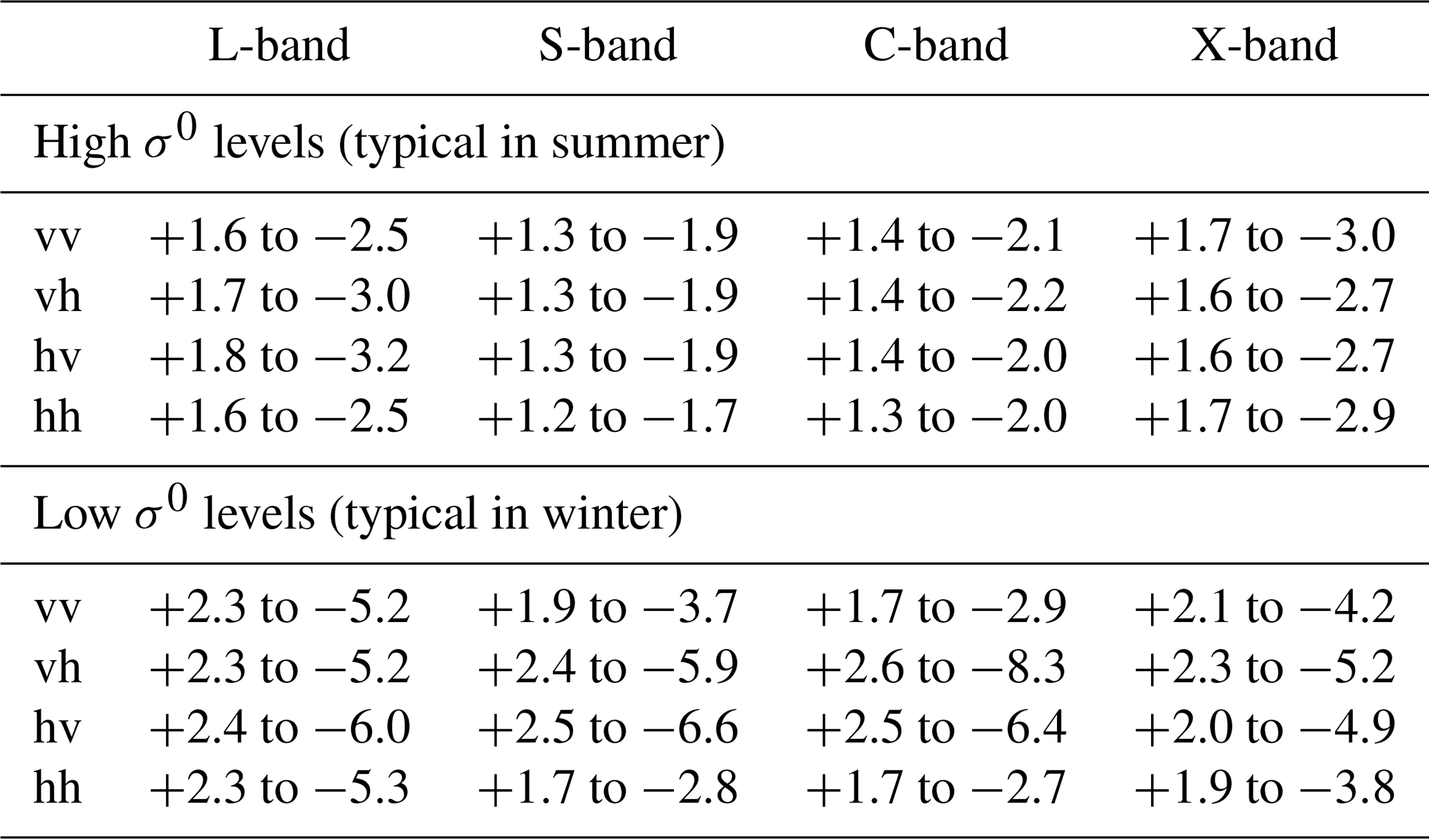
ΔIN (W m−2) is a statistical error that follows from ΔET, ΔK is converted from a maximum possible error into a statistical error with a probability confidence interval, and the term represents a statistical error caused by fading. In the right term the three uncertainty contributions are merged into one statistical uncertainty Δσ0 (m2 m−2), which is a 66 % confidence interval for σ0. In this paper these 66 % confidence intervals are presented in all figures showing our retrieved σ0. To give an indication of the magnitude of Δσ0, some typical values over band, polarization, and season are summarized in Table 2. Presented values were retrieved from the calculated time-series results of Sect. 4.
Table 2Example uncertainty values Δσ0 (dB) per bandwidth, polarization, and overall σ0 level.
The low-directivity-induced uncertainty (iv) is not quantifiable in the sense that with the time-series experiments backscatter was not repeatedly measured at different α0 angles. With such measurements, sets of would be obtained that can be deconvolved into σ0(θ), since G(α,β) is known (see Eq. 2). This deconvolution approach was performed by, for example, Axline (1974) and Ulaby et al. (1983). It is possible, however, to give an estimate of the low-directivity-induced uncertainty, inherent to our σ0 retrieval method, with a simple numerical experiment in which the scatterometer radar return is simulated (Eq. 2) using a pre-defined function for σ0(θ). We may use for example the empirical model of for grassland developed in Ulaby and Dobson (1989) with measurement data from several other studies. Applying the method of Sect. 3.2.3 on the simulated radar return, we obtain for 4.75 GHz at vv polarization dB for , while the actual value over this interval varies from dB. Although this discrepancy depends on the (unknown) form of σ0(θ), in general this error will be larger for low frequencies and smaller for high frequencies because of the respective antenna beamwidths, which has to be kept in mind when using the σ0 values of this dataset. Despite this uncertainty, the σ0 retrieved in this dataset nevertheless does show all relevant temporal dynamics that are furthermore wavelength and polarization dependent.
Alternatively, the low-directivity-induced uncertainty can be avoided by using the radar return of the dataset together with a microwave scattering model instead of the retrieved σ0. The angle-dependent then may be obtained by the microwave scattering model and simply applied in Eq. (2) to simulate the radar return, which subsequently can be compared to the measured values.
5.3 Angular variation of in Maqu
Next, we present the measurement results and analysis of the angle-dependent backscatter of the Maqu site surface for two purposes. First, we present it to quantify the behaviour of σ0 with respect to the elevation angle (θ), BW, and polarization channels for the Maqu site ground surface with a living vegetation canopy, and, second, we present it to assess the spatial homogeneity of σ0(θ) over the Maqu site surface by also measuring backscatter at different azimuth angles (ϕ). As explained in Appendix Sect. C2, the single footprint area for the σ0 time-series measurements should be representative for the whole Maqu site surface. Due to practical limitations of possible ϕ angles and because of the wide antenna beamwidths, the footprints of used α0 and ϕ combinations in this experiment overlap partially, as is shown in Fig. 2. However, since we employ frequency averaging to reduce the fading uncertainty for every footprint, we argue that the σ0 values retrieved per (overlapping) footprint may nevertheless be compared to each other for this section's analysis.
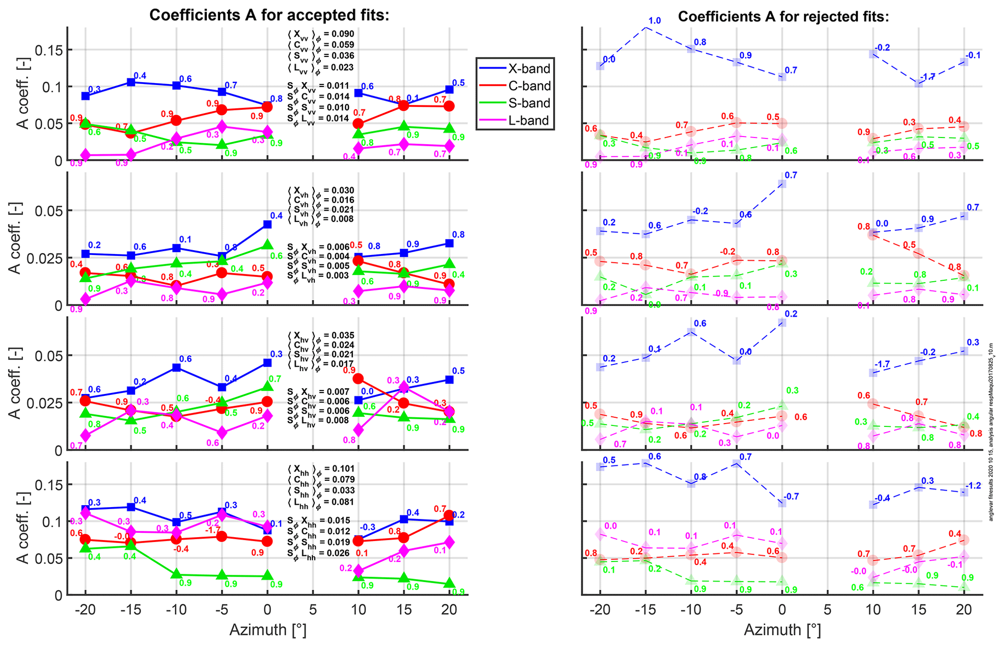
Figure 7Results of fitting the derived values over α0 to model σ0(θ)=Acos (θ)B for different azimuth angles ϕ, bandwidths BW, and polarization channels. The left column shows found coefficients A over ϕ for best fits with the favourable B value for each BW and polarization, and the right column shows the A coefficients with the less favourable B values. Numbers at data points indicate coefficient of determination (R2) of individual fits. Values in the centre are average 〈Bpq〉ϕ and standard deviation SϕBpq over ϕ, with , or X as bandwidth.
As a means to quantitatively evaluate the σ0 behaviour with respect to the θ and ϕ angle, the data are grouped in sets of σ0 over α0 for every angle ϕ, BW, and polarization. In Appendix Sect. G, Fig. G1 examples of such sets are shown. Next, an iterative least-squares non-linear fitting algorithm is applied to fit each set to the model:
where A is a constant (m2 m−2) and B is either 1 for an isotropic scatterer or 2 for a surface in accordance with Lambert's law (Clapp, 1946). For each α0 we find the coordinate for which is maximum and use that position's angle of incidence θ together with the centre σ0 value of the 66 % confidence interval for the fitting process. As a next step, we reduced the number of fitting possibilities by selecting for each polarization–BW combination the most likely value for B (1 or 2). This was done by tallying over the ϕ angles which of the two fitted curves σ0=Acos (θ)B passed through the confidence intervals best and had the highest coefficients of determination (R2). The outcome was B=1 for all polarization channels of X-band and B=2 for all of S- and L-band. For C-band it was harder to judge in favour of either. We chose B=1 for vh polarization and B=2 for vv, hh, and hv. An overview for found parameters A and B is presented in Fig. 7. The stronger decrease over angle found with L- and S-band (B=2) is as expected since for longer wavelengths there is less volume scattering from the vegetation canopy and the soil reflections become more dominant. For these longer wavelengths the soil surface roughness appears smoother, causing specular reflection to be stronger and non-specular reflections (including in the backward direction) to decrease more rapidly with θ. This effect is well known; see for example de Roo and Ulaby (1994). By the same logic, for X-band σ0 will decrease more slowly over θ (B=1) as scattering from the vegetation canopy becomes dominant over that from the soil surface. Strong vegetation scattering is known to be more constant over θ (see for example Stiles et al., 2000), and thus the model for an isotropic scattering surface, i.e. B=1, is more suitable. With C-band both B=1 and B=2 fitted best for about half of the ϕ angles, which indicates that at this intermediate wavelength we see both aforementioned features. With the co-polarization channels we see that the average A values over ϕ decrease with increasing wavelength as expected considering the description above. An exception, however, is the L-band response with hh polarization, which is comparable to that of C-band. As with the asphalt measurements (Appendix Sect. 5.1), we believe these high σ0 retrievals are due to the low angular resolution of our scatterometer for L-band. As a result, the backscatter for close to nadir angles (which are highest in general) is present in all angular positions α0. This is visible in the inset figure of Fig. G1. We also note that the variation over ϕ (by comparing SϕBpp to 〈Bpq〉ϕ) is smallest for X-band and largest for L-band. The cross response is lower than that for the co-polarization as expected. For both vh and hv the X-band backscatter is also largest here, while the cross-polarization backscatter for L-band is lowest. However, S-band appears to have stronger backscatter than C-band. We do not have a clear explanation for this. As with the co-polarization channels the variation over ϕ is strongest for the longer wavelengths.
Finally some remarks on the variation of A over ϕ and, virtually, across the surface area. Except for X-band with hh polarizations there did not appear to be a systematic trend of A over ϕ. Also, there was not one particular ϕ angle for which the values for A over BW and polarization stood out from the rest. These observations indicate that the surface area covered by our scatterometer appeared to have uniform (scattering) properties. The somewhat higher A values with the negative ϕ values with X-band at hh polarization are probably caused by a difference in vegetation density between the left and right side of the Maqu site. Fortunately, for the A value had a medium value compared to the other ϕ angles, so that we may still interpret the surface area associated with the scatterometer's (fixed) footprint during the time-series measurements as being representative for its surroundings.
In the DANS repository, under the link https://doi.org/10.17026/dans-zfb-qegy, the collected scatterometer data are publicly available (Hofste et al., 2021). Stored are both the radar return amplitude and phase for all four linear polarization combinations and processed for the L-, S-, C-, and X-band bandwidths discussed in this paper. The dataset includes time-series measurements from 26 August 2017–26 August 2018, data of angular-variation experiments, and radar returns of the reference targets. Accompanying data include time-series measurements of soil moisture and temperature profile at depths of [2.5, 5.0, 7.5, 10, ... 90, 100 cm], as well as time-series measurements of air temperature, precipitation and up- and downward short- and long-wave irradiation. Note that the volume of the dataset is too large (20 GB) to disseminate via DANS' web interface. Users are to contact the DANS repository, after which DANS will establish an alternate file transfer. Also, in the DANS repository under https://doi.org/10.17026/dans-xyf-fmkk (Hofste, 2021), MATLAB scripts are available for processing measured radar return data and for retrieving for other bands within the measured 1–10 GHz frequency range.
A ground-based scatterometer system was installed on an alpine meadow over the Tibetan Plateau and collected a 1-year dataset of microwave backscatter over a broad 1–10 GHz band for all four linear polarization combinations.
Measurements of the incidence angle dependence of for asphalt agreed with previous findings, thereby showing our σ0 retrieval method to be accurate. Presented analysis on the angle-variation data of σ0 in Maqu showed wavelength- and polarization-dependent scattering behaviour due to vegetation that is in accordance with theory and other studies. Furthermore, these measurements indicated the Maqu ground surface to have spatially homogeneous electromagnetic properties and the area associated with the (fixed) footprint for the time-series measurements to be representative of its surroundings.
The uncertainty of our retrieved σ0 consists of quantifiable parts estimated from fading and systematic measurement uncertainties and an unknown part due to the low directivity of used antennas. The quantifiable uncertainty in σ0 was estimated with an error model providing 66 % confidence intervals that are different over frequency bands, polarizations, and the overall level of the radar return. Typical Δσ0 values during summer range from ±1.5 dB for S-band with hh polarization to ±2.5 dB for L-band with hv polarization. Despite aforementioned uncertainties in σ0 we believe that the strength of our approach lies in the capability of measuring σ0 dynamics over a broad frequency range, 1–10 GHz, with high temporal resolution over a full-year period.
Our preliminary analysis on the retrieved for L-, S-, C-, and X-band demonstrates that the scatterometer dataset collected at fixed time intervals over a full year at the Maqu site contains valuable information on exchange of water and energy at the land–atmosphere interface — information which is difficult to quantify with in situ measurement techniques alone. Hence further investigation of this scatterometer dataset provides an opportunity to gain new insights in hydrometeorological processes such as freezing and thawing, or wavelength-dependent scattering effects in the vegetation canopy during spring and summer periods.
A1 Photographs of the site phenology
In this section we present a set of photographs (see Fig. A1) of the Maqu site taken at different seasons since the installation of the ELBARA-III in January 2016. These may give the reader a global indication of how the site phenology changes throughout the seasons.
A2 Hydrometeorological sensors and measurement results
Table A1 lists all hydrometeorological instruments used for this study along with their reported measurement uncertainties. Air temperature was measured with a platinum resistance thermometer, type HPM 45C, installed 1.5 m above the ground, and precipitation (both rain and snow) was measured with a weight-based rain gauge, type T-200B.
We formulate in brief our main observations over the measured hydrometeorological quantities at the Maqu site over the period 26 August 2017–26 August 2018. Figure A2 provides an overview with a 2 d temporal resolution. All data are available in the dataset with a temporal resolution of 30 min.
The lowest air temperatures Tair were measured in January 2018, during which daily minimum values dropped below −20 ∘C, while daily maximum temperatures did not rise above 0 ∘C. In July–August 2018 Tair was highest, with maxima above 20 ∘C.
Soil temperature Tsoil and soil volumetric liquid water content mv varied over depth. Depending on the amount of liquid water in the soil, the penetration depth of frozen soil at L-band can vary from 10–30 cm at the Maqu site (Zheng et al., 2017a). We consider Tsoil and mv values at 25 cm depth, which is closest to the maximum aforementioned penetration depth. From the measurements we conclude that at 25 cm depth the soil can be considered frozen between 21 December 2017–5 April 2018 (arrows in figure). For other depths the freezing and thawing process is substantially different from the shown curves. During the 2017–2018 winter Tsoil dropped below 0 ∘C up to a depth of 70 cm (not shown in Fig. A2).
Total precipitation over the considered 1-year period was 688 mm. The majority of this amount fell in the months of September and October 2017 and in August 2018, while from November 2017 to the middle of March 2018 there was only 7 mm precipitation. Presence of snow on soil was inferred from the observed noon albedo to be 0.4 or higher.
A3 Derivation of spatial soil-moisture-variation estimate
This section describes how the spatial average soil moisture content over the Maqu site Mv (m3 m−3) is linked to mv as measured by the 5TM sensors at 2.5 and 5 cm depth.
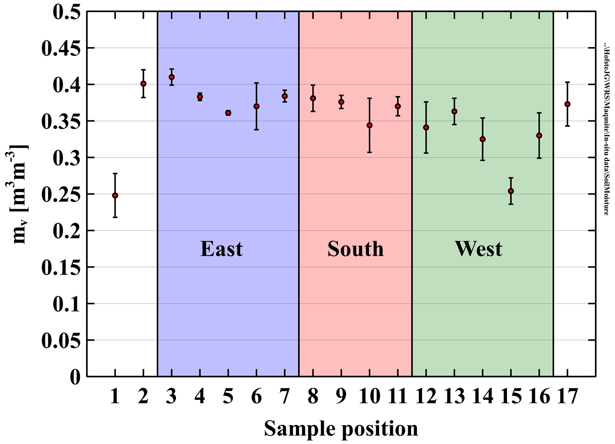
At every depth, mv varies over the horizontal spatial extent at all scales (Famiglietti et al., 2008). Local mv variability is caused by variations in soil structure and texture, including organic matter. At the Maqu site, the 5TM sensor array forms only one spatial measurement point for soil moisture. We denote its measurements as (m3 m−3). In an attempt to quantify how at the top soil layer (depths 2.5 and 5 cm) relates to the soil moisture over the rest of the Maqu site, we sampled mv at 17 positions along the no-step zone (Fig. 2) on 29 June 2018 with a handheld impedance probe, type ThetaProbe ML2x, whereby three measurements were taken per position. Figure A3 shows the measured mv in the top layer. Taking aside the outlying values at positions 1 and 15, we observe that the variation along the periphery is slightly larger than the variability amongst the three measurements taken at a specific position. The average standard deviation over the 15 positions is 0.03 m3 m−3, while the average standard deviation over the three measurements is 0.02 m3 m−3. Given this small difference we concluded there is no clear spatial trend of top soil mv at the Maqu site. Therefore, we considered all readings as independent measurements on spatial mv variation, which we used to determine the quantity Stot (m3 m−3), called the total standard deviation of spatially measured mv. Stot is an estimate for the spatial mv variability over the Maqu site. Subsequently, we use Stot to relate the measured to the spatial average top soil moisture content over the Maqu site Mv (m3 m−3) according to
Using the assumption of temporal stability of spatial heterogeneity (Vachaud et al., 1985), we consider the found Stot to hold throughout the year. Stot is calculated by
according to standard error propagation theory (see for example Hughes and Hase, 2010). The term Ss (m3 m−3) represents the spatial mv variability as measured along the periphery. It is calculated as the standard deviation over 45−1 samples and is 0.031 m3 m−3. The standard deviation S5TM has value of 0.02 (m3 m−3) and is the root-mean-square measurement error of the 5TM sensors. It was derived in Zheng et al. (2017b) after calibrating 5TM sensor retrievals to top soil gravimetric soil samples taken at the Maqu site. The term Sp is the propagated error of the 0.05 m3 m−3 theta probe measurement accuracy (Table A1) when Ss is calculated. m3 m−3. Finally, Stot then is 0.04 m3 m−3.

Figure A1Maqu site changing phenology. (a) Winter, January 2016. (b) Spring, 16 May 2017. (c) Spring, 26 June 2018. (d) Summer, 17 August 2018. (e) Winter, 6 January 2018. (f) Winter, 6 January 2018.
Table A1Overview of relevant hydrometeorological sensors at the Maqu site.
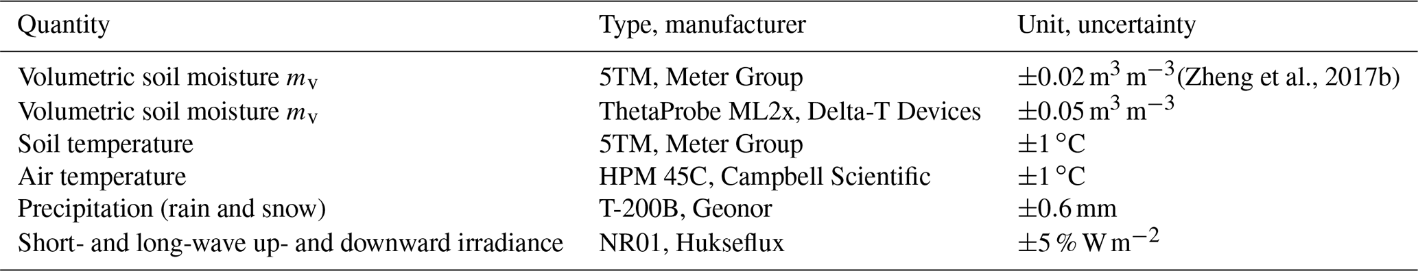
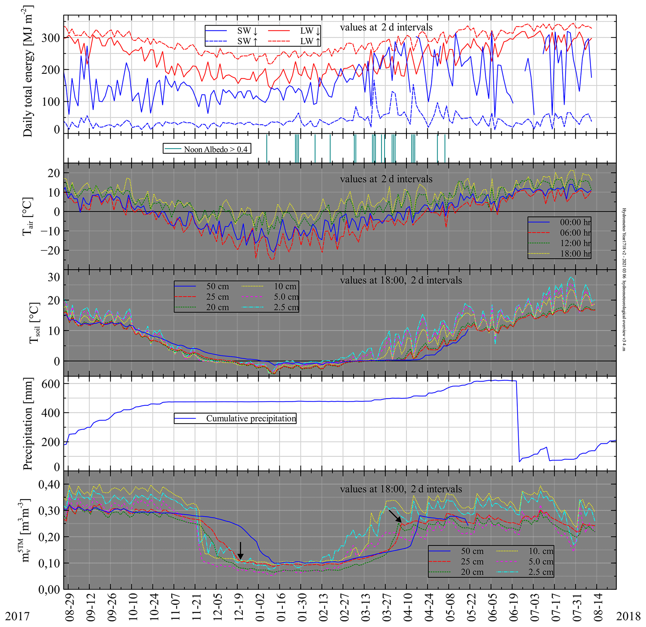
Figure A2Overview of hydrometeorological quantities measured at the Maqu site over the period 26 August 2017–26 August 2018. From top to bottom: daily total sum of down- and upward hemispherical energy (MJ m−2) for short (285–3000 nm) and long (4500–40 000 nm) wavelengths at 2 d intervals, days with snowfall (identified from noon albedo), air temperatures (∘C) at four times during the day at 2 d intervals, soil temperatures Tsoil (∘C) for different depths at 2 d intervals, cumulative precipitation mm, and volumetric soil moisture m3 m−3 for different depths at 2 d intervals. Arrows indicate freeze/thaw of soil at 25 cm. Spatial average volumetric soil moisture Mv is estimated as m3 m−3.
A4 Vegetation sampling
Table A2Measured vegetation parameters at the Maqu site during summer 2018. Vegetation water content (VWC) is gravimetric: kilogram of water per kilogram of fresh biomass.
B1 Connection scheme and VNA operation
In Fig. B1 the connection scheme that was used is shown. The front-panel jumpers were removed, and the two dual-polarization broad-band horn antennas were directly connected to the VNA's sources and receivers via the four coaxial cables. This configuration allows for measuring all four polarization channels: vv, vh (i.e. receive in the vertical direction, transmit in the horizontal direction), vh, and hh (Keysight Technologies, 2017). Between all four coaxial cables and their respective VNA connectors, 10 dB attenuators, type SMA attenuator R411.810.121 (manufacturer: Radiall), were inserted to prevent interference from internal reflections travelling multiple times up and down the coaxial cables.
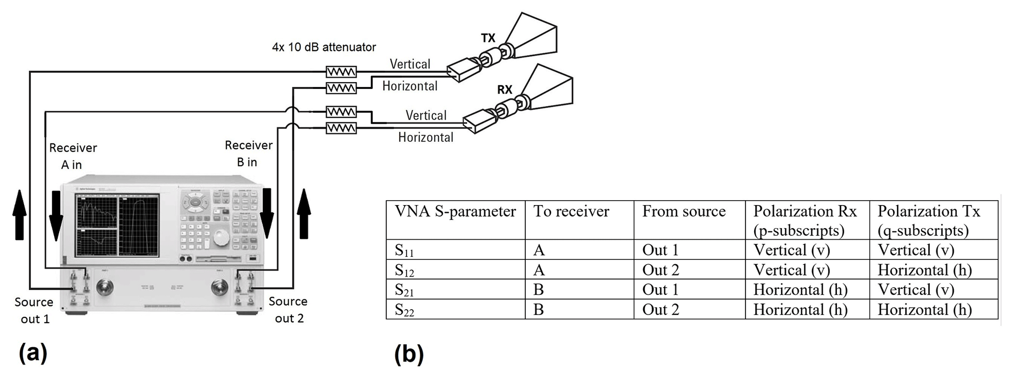
Figure B1Connection scheme of scatterometer and correspondence S parameters to polarization channels for transmit (TX) and receive (RX). (a) Both dual-polarization broad-band antennas, one for TX and the other for RX, are connected to the VNA as indicated (Keysight Technologies, 2017). Arrows indicate direction of signal. (b) Overview correspondence of four VNA S parameters to the four polarization channels.
Measurements were performed by instructing the VNA to measure the four scattering parameters (S parameters)2 (–) over a stepped frequency sweep 0.75–10.25 GHz. Given the aforementioned connection scheme, the correspondence between recorded S parameters and transmit/receive polarization channels is as indicated in Fig. B1b. The used connection configuration omits the VNA's internal test-port couplers, which are typically used when measuring (two-port) S parameters. The VNA software – by default – accounts for these test-port couplers by adding 16 dB to the signal measured by receivers A and B when calculating the S parameters. With the σ0 retrieval, this 16 dB amplification cancels out as the target is divided by the reference return. However, when considering the received powers individually, as done in Sect. 5.2, this factor should be accounted for.
B2 Geometries of experimental setup
Figure B2a shows all relevant geometries for the performed experiments. The two antenna apertures are at distance Hant above the ground surface. The separation between the two antenna apertures Want=0.4 m is small compared to the target distance (ground or calibration standards), which justifies using the geometric centre of the two apertures for all calculations. Every area segment dA (m2) of the ground surface has its own distance to the antennas R and angle of incidence θ. Angles α and β are angular coordinates of R. Angle α is defined between the tower's vertical axis and the orthogonal projection of the line from antennas to a ground surface segment onto the plane formed by the tower's vertical axis and the antenna boresight direction line. Angle β is defined between the line from antennas to a ground surface segment and projection of that same line onto the plane formed by the tower's vertical axis and the antenna boresight direction line. The planes in which α and β lie are also the antenna's principal planes (see for example Balanis, 2005). For the antenna boresight direction α=α0 and β=β0. The antenna rotation around the tower's vertical axis is defined as azimuth rotation ϕ. The green ring on the ground surface in Fig. B2a is related to the time-domain gating process described further on in Sect. B4.
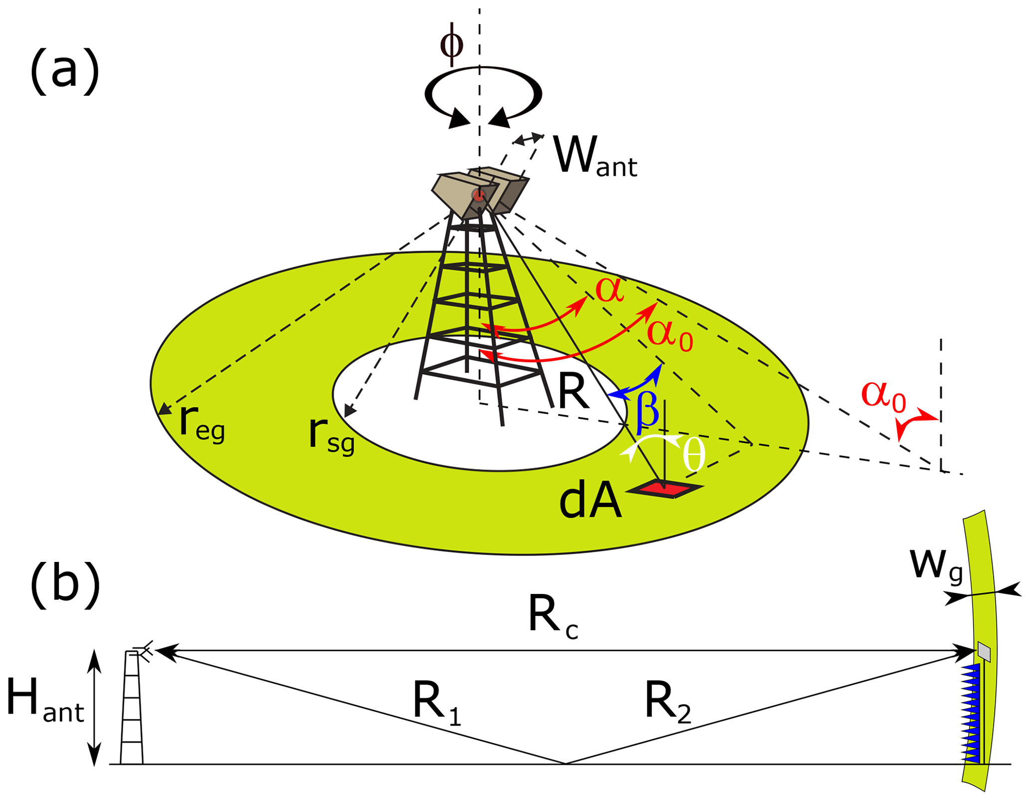
Figure B2Schematic of scatterometer geometry. (a) Every infinitesimal area dA has its own distance R to the geometric centre between antenna apertures (red dot) and angle of incidence θ. Angles α and β lie within the antennas principal planes, and α0 denotes the angle of antenna boresight. The green ring is a projection of the spherical gating shell with radii rsg and reg onto the ground. (b) Side view of geometry during measurement of reference standards. Green ring depicts cross section of spherical gating shell with width wg.
According to Bansal (1999) the antenna's far field distances Rff (m) are linked to the antenna's largest aperture dimension D (m) and wavelength λ via
The antenna aperture is rectangular with dimension D=0.2 m, which leads to Rff≥1 m for 1–3.5 GHz and Rff≥2.7 m for 3.5–10 GHz. Given that with all measurements the distance to the ground surface is larger than 2.7 m, the radiation patterns as measured by the manufacturer apply; see Fig. B3 (Schwarzbeck Mess-Elektronic OHG, 2017).
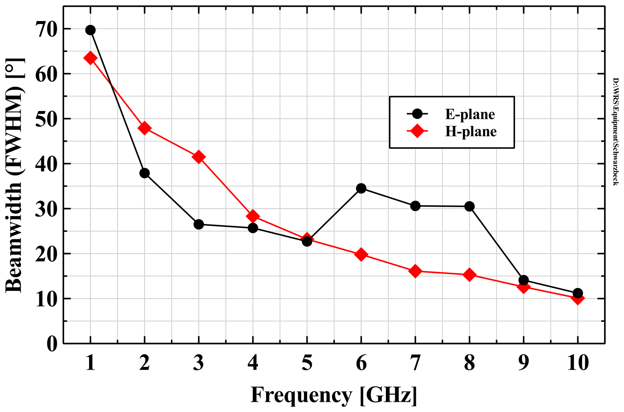
Figure B3Beamwidths of dual-polarization antennas. Shown is the full width at half maximum (FWHM) of the measured radiation intensity patterns in the two principal planes (Schwarzbeck Mess-Elektronic OHG, 2017).
Figure B2b shows a side view of the setup when radar returns of the reference targets were measured in order to calibrate the scatterometer. The reference targets – a rectangular metal plate and two metal dihedral reflectors – were placed at distances R0 from the antennas on top of a metal mast. To shield this mast, pyramidal absorbers were placed in front of it as shown. Next section describes the calibration process in detail.
B3 Calibration
We measured the radar returns of reference targets with known radar cross section (RCS) σpq in order to calibrate the scatterometer. For the co-polarization channels a rectangular metal plate was used as reference target. As a depolarizing reference target for the cross-polarization channels we used a metal dihedral reflector that was rotated 45∘ around the axis perpendicular to the vertex connecting the dihedral's two faces and contained in the symmetry plane also holding the same vertex. The physical optics model used for calculating the RCS of a metal plate and dihedral reflector is
where a and b are the standards' dimensions (m) in the frontal projection (Kerr and Goldstein, 1951). As is shown in for example (Nesti and Hohmann, 1990), Eq. (B2) is also applicable for calculating the cross-polarization RCS of the dihedral reflector when in its rotated position.
Table B1Deployed reference standards and their bandwidths of validity concerning plane wave (PW) and size-to-wavelength criteria.

There are validity conditions for model (B2) which concern the reference target's size and the distance at which it is measured R0. Additionally, the multi-path field illumination of the reference targets (Skolnik, 2008) might be an issue: besides direct illumination from the transmit antenna, radiation reflected from the ground will also illuminate the target; see Fig. B2b. As a result, the direct signal is interfered by these ground-to-target reflections. Table B1 lists R0 values used for the deployed reference standards. We first describe the validity conditions for model (B2).
Conditions for Eq. (B2) are that the standard's largest dimension L (m) is large compared to the wavelength, i.e. L>λ, and that the incident wavefront is close to planar. Kouyoumjian and Peters (1965) proposed the following equation for calculating the minimum distance Rpw (m) beyond which the wavefront can be considered planar (allowing for a phase error):
Concerning the condition L>λ, previous measurements (Hofste et al., 2018) showed, empirically, that for model (B2) matches a standard's measured σpp within 1 dB. Besides the R0 values used, Table B1 also lists the frequency ranges for which the plane wave criteria (using the stated values R0) and the size criteria hold. Strictly speaking, the plane wave criteria with the rectangular plate was not met for 7.5–10 GHz. Yet, the co-polarization σ measurement of the small dihedral reflector, discussed in Sect. E3.2, yields results close to the Eq. (B2) value, indicating correct values for 7.5–10 GHz.
Now we discuss the possible issue of multi-path illumination by ground-to-target reflections (GTRs). Should the signal strength of these GTRs be significant, the magnitude-over-frequency response of the reference targets will exhibit interference ripples, which complicate interpreting their radar return for the purpose of calibrating the scatterometer. By using gating the GTRs could in principle be removed from the direct target response, provided their difference in geometrical path length is large enough for placing a gating window solely over the direct path reflection in the time domain. The GTR path shown in Fig. B2b was the pathway whose path length was closest to that of the direct route. Also, this GTR path will have the strongest coherent ground reflection since it is specular. Naturally, with smaller R0 the difference increases, allowing one to better distinguish this GTR from the mean reflection.
However, no (clear) presence of any GTR could be found. Using a BW=0.5 GHz bandwidth leads to a ns resolution in the time domain, which would allow us to see the shortest GTR-path reflection that – if present – should be at ns behind the direct-reflection peak. But even with S-band for hh polarization (broad antenna pattern, and for hh polarization the coherent ground reflection is strongest) no GTR could be found.
Because we could not find evidence of GTR interference we hypothesize that the GTRs were too small in magnitude for our case. The antenna patterns, certainly for the lower frequencies, are broad enough to illuminate a large part of the ground surface, but because of the dense grass cover the coherent forward reflections were probably low. Additionally the bistatic-RCS patterns of both the rectangular plate and dihedral reflector are too narrow, even with L-band, for a sufficient amount of energy to be reflected (in a specular manner) back to the receive antenna. Typically the presence of interference due to multi-path illumination with setups like ours is tested by moving the reference target horizontally over a distance of half a wavelength and observing any changes in the signal. Unfortunately this procedure was not possible with our equipment.
B4 Gating
For simplicity, instead of using the (complex) electric-field strength measured at the scatterometer's receive antenna Ee, we explain the gating process with the term X (V), which can be considered proportional to Ee by some scatterometer system constant. The measured frequency domain signal X[ωh] was transformed into the time domain via the inverse digital Fourier transform (IDFT); see for example Tan and Jiang (2013):
N is the total number of discrete frequency points within the bandwidth BW (Hz) considered. Angular-frequency points ωh (rad s−1) and time points tn (s) are calculated with the minimum and maximum frequency of BW, flo and fhi respectively (Hz), via
Next the time-domain response x[tn] was multiplied by the time-domain filter, or gate, which was a block function of width τg whose sides fell off according to a rapidly decaying Gaussian function, zeroing all signal parts not coinciding with the unity values. The gate's start and end times corresponded to the distances indicated in Fig. B2a: and respectively; so in effect, only the surface's scattering events of interest remained in the signal. Graphically, this process is displayed in Fig. B2a. When assuming isotropic radiating and receiving antennas, selecting a certain time gate is equivalent to only considering scattering events within a spherical shell, centred at the antennas, with radii rsg and reg. The intersection of said shell with the ground surface then is a ring as shown in the figure. However, our actual antennas have non-isotropic radiation patterns. So they are in fact the surface scattering events associated with the area formed by the intersection of the shown green ring and the scatterometer footprint Afp that are contained in the signal. As the next step, the gated signal x[tn] was transformed back into the frequency domain via the digital Fourier transform (DFT):
which then contains only the surface scattering information.
The frequency dependence of the radiation patterns, as shown in Fig. B3, complicates the process described above. The time-domain equivalent of the transmitted scatterometer signal is a pulse of width s. Depending on the angle with respect to boresight, i.e. α and β, this signal pulse will contain different frequencies and will therefore have a different temporal shape. At greater angles α and β, high-frequency components of the pulse are not present, causing the pulse to be broader there. As a result, the footprint area Afp, which is determined from the (known) antenna radiation, or gain patterns G and the gate width wg=cτg will become broader. We avoided this issue by narrowing our bandwidths such that the radiation patterns of the frequencies within can be considered equal. As a consequence, this meant that for lower frequencies the selected BW had to be more narrow than those for the higher frequencies. The bandwidths used were 1.5–1.75 GHz for L-band, 2.5–3.0 GHz for S-band, for 4.5–5.0 GHz for C-band, and for 9–10 GHz for X-band. Note that there were additional considerations for picking these BW values, which are explained in Sect. C2.
When measuring the reference target backscatter responses E0 (V m−1), however, the full 0.75–10.25 GHz frequency range can be used. Because the solid angle extending the standard is small we may reasonably assume that all frequencies are present in the time-domain equivalent pulse at the standard, i.e. for all frequencies. The benefit of using this broad bandwidth (9.5 GHz) is a high temporal–spatial resolution in the time domain, which allows for precise placement of the gate over the reference target response.
C1 Implementation of the radar equation
We rewrite Eq. (3) so that the backscattering coefficient of the surface σ0 (m2 m−2) is related to the average received backscattered intensity (Wm−1) as (Ulaby and Long, 2017)
where for brevity the polarization subscripts are omitted. The factor K (W m−1) is a constant for the bandwidth considered given by
where It (W m−2) is the transmitted intensity by the scatterometer. For all terms in K the centre frequency is used. Similar as with Eq. (2), we can substitute It in Eq. (C2) by the relevant radar parameters when a reference target is measured, yielding
(V m−1) is the measured backscattered field from the reference target (subscript 0 represents “reference”), and (V m−1) is the measured background level during calibration, i.e. the measured backscattered electric field when the calibration standard was removed from the mast while the pyramid absorbers remained in place. With both terms the superscript g0 (for “gate” during reference measurements) indicates that an identical gate was used. The field strength associated with the minimum signal level measurable with the scatterometer is denoted Eb (V m−1). The prefactors light speed c (m s−1) and the permittivity of vacuum ϵ0 () convert the electric-field strengths into time-average intensity. In the middle part of Eq. (C3) the antenna gain functions are written explicitly. G(α,β) represents the antenna gain functions when measuring the ground return, while G(α0,β0) represents the situation when the radar return of the reference targets is measured. When using the narrow beam approximation (Eq. 3) and when the reference target is aligned to the antenna boresight direction, the fraction becomes unity and the right part of Eq. (C3) follows. The middle part is used in Appendix Sect. E3.1 when alignment uncertainty of the reference targets is discussed.
In the context of Rayleigh fading statistics with square-law detection (Ulaby et al., 1988), the average received intensity (W m−2) is linked to IN (W m−2), which is the measured intensity averaged over N independent samples (N footprints or N frequencies), according to
Note that , like σ0, is an implied ground surface property. The quantity that is actually measured, IN, is an estimator for . Equation (C4) holds for N≥10, since then the probability density function of IN approaches a Gaussian distribution (Ulaby et al., 1982) according to the central limit theorem. The denominator in Eq. (C4) represents a 68 % confidence interval (±1 standard deviation) for . More details on fading are described next in Sect. C2.
In turn, IN is calculated from the measured backscattered electric field from the ground target incident on the receiving antenna (V m−1) by
C2 Fading and bandwidth selection
Fading is the phenomenon where radar return of a distributed target with uniform electromagnetic properties has varying magnitudes and phases when different locations or slightly different frequencies are measured (Ulaby et al., 1988; Monakov et al., 1994). To remove this varying nature from a surface-classifying quantity like , averaging must be performed. By definition is the average radar cross section of a certain type of distributed target, e.g. forest, asphalt, wheat field, normalized by the illuminated physical surface area. σ0 is proportional to the average measured received power PRX (Eq. 3) or intensity . Therefore, determining and σ0 requires N statistically independent samples so that the sample average IN approaches the actual average proportionally to in accordance with the central limit theorem.
Practically, this can be done either by measuring I at N different locations over the surface, called spatial averaging, or with the frequency averaging technique (see for example Ulaby et al., 1988). With the latter, physical properties governing the scattering, permittivity, and surface roughness are considered frequency invariant over a certain bandwidth. Subsequently, N different frequencies should be selected according to some criteria that account for fading. Both averaging techniques can be used simultaneously as done by Nagarajan et al. (2014) to increase the total number of independent samples. We solely applied the frequency averaging technique because during the time-series measurements our antennas were in a fixed position and orientation. We assumed the single footprint area to be representative for the whole surface of the Maqu site. In Sect. 5.3 we show this assumption is justified. The method used for finding the number N of statistically independent samples within a bandwidth BW is described in Mätzler (1987):
where . Subsequently, with N−1 intervals of Δf (Hz), N frequencies are selected from within BW.
As indicated above, with the application of the frequency averaging technique it is assumed that the backscatter behaviour across the selected BW is uniform. To assess the validity of this assumption for bare soil surface, the improved integral equation method (I2EM) surface scattering model (Fung et al., 2002) is applied using the roughness parametrization reported in Dente et al. (2014) and a (frequency-dependent) effective dielectric constant ϵsoil(f) according to the dielectric mixing model by Dobson et al. (1985).
Over a BW the mean value 〈σ0(BW)〉 is calculated, followed by the ratios and to quantify the change in σ0 over the BW. In general the I2EM model predicts that the change is largest for long wavelengths and smallest for short wavelengths and that it is largest for hh polarization and smallest for vv polarization. Furthermore, the root-mean-square surface height s (m) is the most sensitive target parameter. As an example, Fig. C1 shows the calculation result for hh polarization with a BW of 0.5 GHz. From the graph we can read that for a centre frequency of 2.75 GHz the retrieved for that BW can be expected to vary +1.0 to −1.2 dB for .
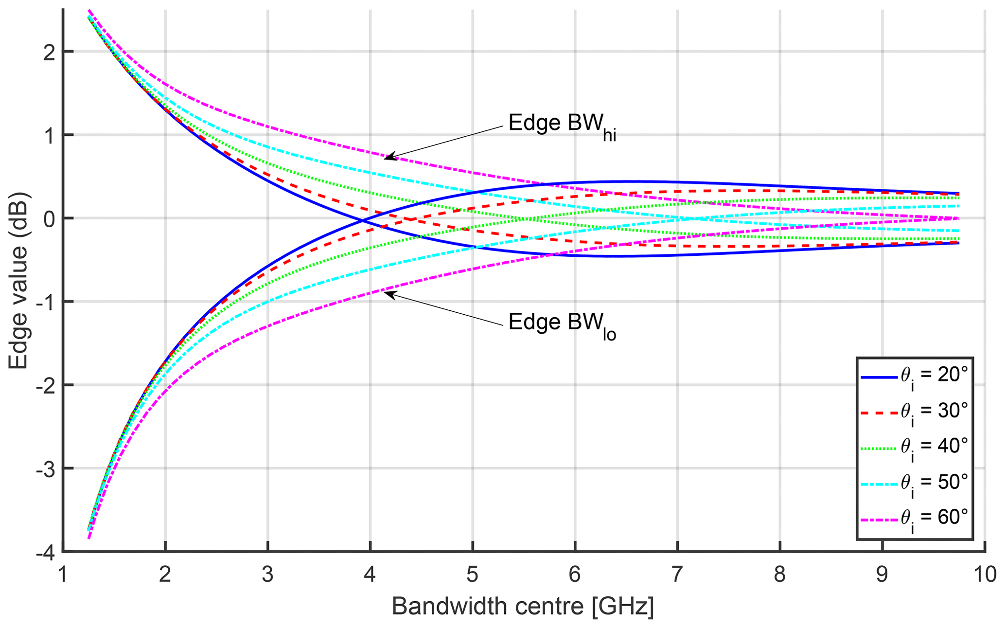
Figure C1Variation of per BW calculated with the combined I2EM (Fung et al., 2002) and Dobson (Dobson et al., 1985) model. The horizontal axis shows centre frequency of bandwidth BW=0.5 GHz. Curves indicate the values (in dB) to be added to at the BW edges for different θ angles. Shown calculation uses: s=1 cm, ℓ=10 cm, mv=0.25 m3 m−3, and Tsoil=15 ∘C.
Based on the above calculations we chose BW=0.25 GHz for L-band, BW=0.5 GHz for S- and C-band, and BW=1.0 GHz for X-band. These bandwidths will lead to N values around 10, which is sufficient to let the probability density function of IN approach a Gaussian distribution, as explained in Sect. 3.2.3. Further increment of BW was considered not to outweigh the loss of frequency resolution, especially at S-band.
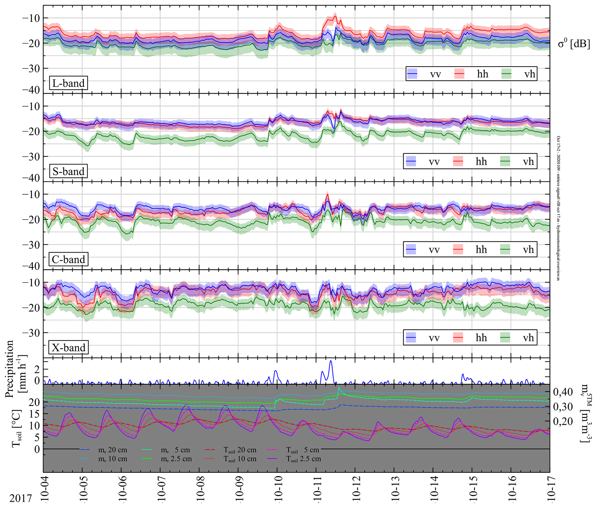
Figure D1Time-series measurements of (m2 m−2) for L-, S-, C-, and X-band, precipitation, Mv, and Tsoil during 13 d in October 2017. Shaded regions indicate 66 % confidence intervals for . The antenna boresight angle was fixed at . The incidence angle ranges were band and polarization dependent. The widest ranges were for L-band, for S-band, for C-band, and for X-band. Bottom graphs show measured precipitation (mm h−1), volumetric soil moisture (m3 m−3), and soil temperature Tsoil at indicated depths. Spatial average volumetric soil moisture content Mv is estimated as m3 m−3.
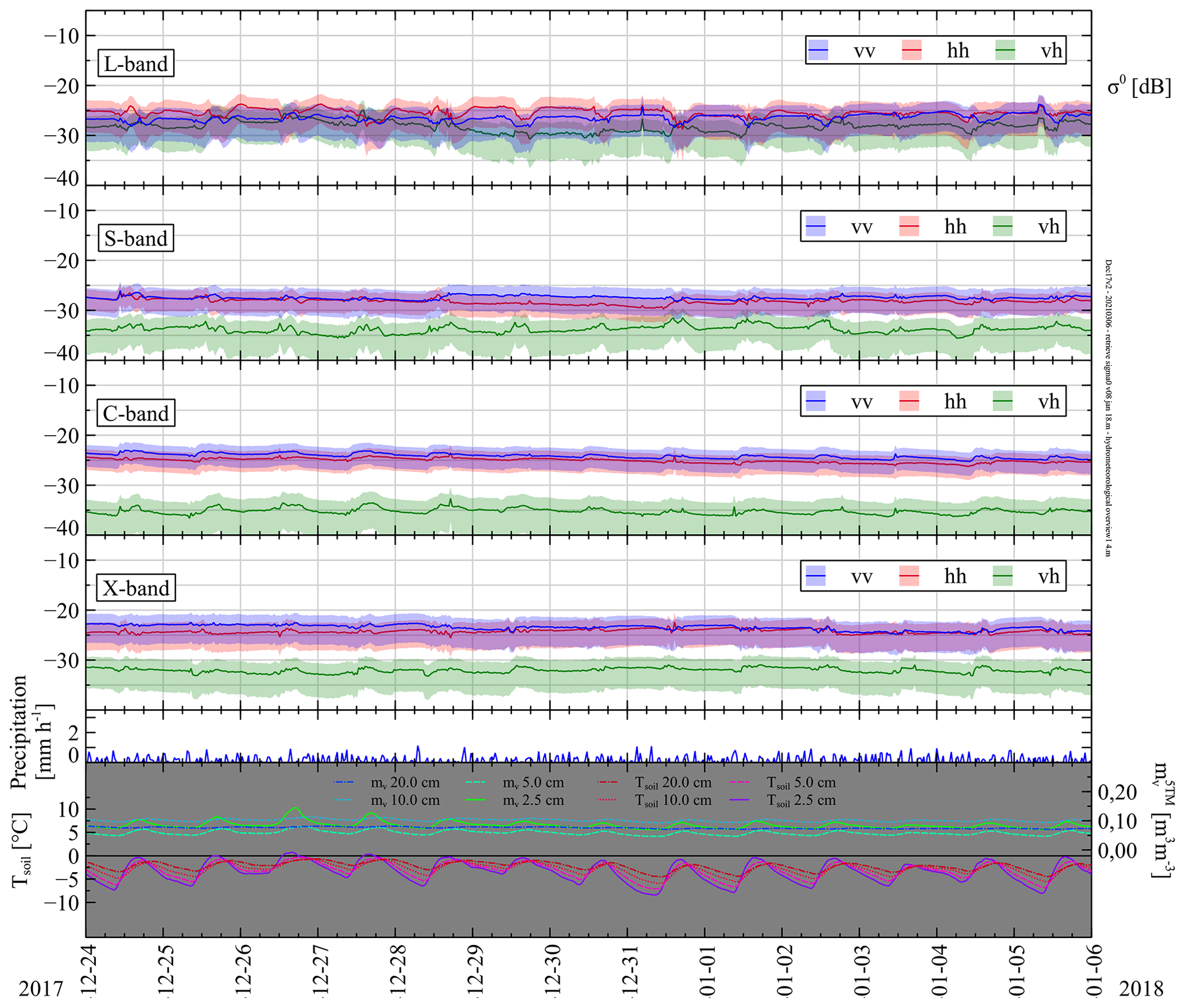
Figure D2Time-series measurements of (m2 m−2) for L-, S-, C-, and X-band, precipitation, Mv, and Tsoil during 13 d in December 2017. Same configurations as Fig. D1 apply.
E1 Overview measurement uncertainty
Table E1 lists all systematic measurement uncertainties and offsets per BW and polarization channel. The uncertainty ΔK (Appendix Sect. E3) and σmin values are shown as is, but for the other quantities the resulting receiver power levels (in dBm) are shown to allow for comparison with other systems. As explained in Appendix Sect. B1 the VNA actually measures the four S parameters, which are the (complex) ratios of the received over the transmitted wave voltage for the four polarization channels. The received wave voltages are proportional to the different electric-field strengths Ee, E0, etc. described in Sect. 3.2.3. The transmitted wave voltage, or actually its power, is constant at 10 dBm with all measurements. For the calculation of σ0 by Eq. (C1) it is irrelevant whether the electric-field strengths, wave amplitudes, or S-parameter magnitudes are used since the transmission-related components and/or prefactors simply cancel out. Conversion from measured S parameters (which are associated with the corresponding scattered electric-field strengths) to receiver power is done by subtracting −16 dB, which was added by the VNA software to account for the test-port coupler, and adding 10 dBm. As an example we consider a ground measurement taken on 24 December 2017 at 00:10:00 LT. The VNA measured dB for 2.8 GHz (S-band) with vv polarization. The power at the VNA receiver then was dBm.
Table E1Summary of systematic uncertainties, offsets, and minimum signal levels. Concerning ΔET, , and Eb, table values are the receiver power levels derived from measured S parameters which, in their turn, are associated with ΔET, , and Eb. With ΔK and σmin actual values are shown.
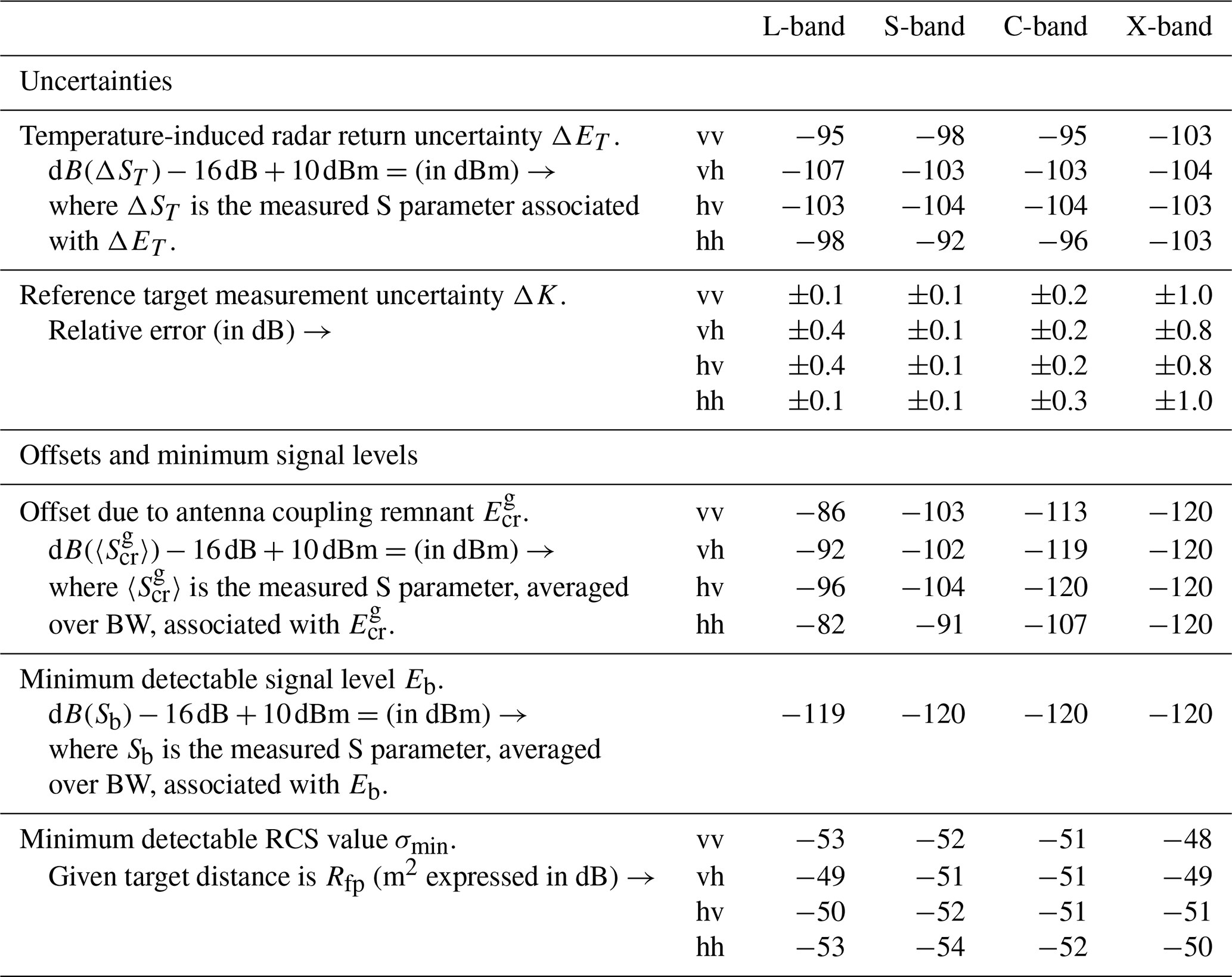
From Table E1 we observe that the received power associated with ΔET (Appendix Sect. E2) and (Appendix Sect. E4) is, in general, highest for L-band and lowest for X-band. Also, the cross-polarization channels have lower values than those for co-polarization. As for ΔET, we do not have a clear explanation for this behaviour. For we argue that the L-band values are highest due to the stronger coupling because of the broadest radiation patterns at that band. The co-values are higher than with cross polarization because of how the electric-field lines allow for better coupling with the former. The power levels associated with Eb were derived from the specifications documentation of the VNA (Keysight Technologies, 2018). The typical receiver noise levels described therein are specified for a 10 Hz IF bandwidth. Since we measured with a broader 1 KHz IF bandwidth we added 20 dB to obtain the values in Table E1. We would like to mention here that the values associated with for X-band and the hv channel of C-band were actually lower than the −120 dBm levels associated with Eb. We do not have a clear explanation for this. We therefore consider the Eb as the absolute minimum signal levels and therefore adjusted the values to this level.
The variation of σmin over the bands and polarization channels is due to the variation in measured values of . Overall the minimum RCS is about −50 m2 (dB). Other studies use the more appropriate so-called noise-equivalent σ0 (m2 m−2) to quantify the minimum detectable (distributed) target; see for example Nandan et al. (2016) or Nagarajan et al. (2014). Because of our broad antenna radiation patterns, however, this quantity is not suitable, and therefore we instead refer to a discrete target extending a small solid angle.
E2 Temperature-induced radar return uncertainty
The performance of the VNA's transmitters and receivers will vary due to variations of their operational temperatures, which in our case are directly linked to the temperature inside the VNA enclosure Tencl. Many scatterometer systems employ a so-called internal calibration loop; see for example Ulaby and Long (2017), Baldi (2014), and Werner et al. (2010). This means that beside, or in between, scatterometer measurements, the transmitter and receiver are connected, via a switch, through a reference transmission line of fixed length that has a pre-determined attenuation and phase. This way any fluctuations in the transmitter and/or receiver output over time can be measured and consequentiality removed from the target response. Instead of such an internal calibration loop we employ a different method to account for temperature-induced fluctuations of the VNA's transmitter and receiver performance.
During a half-day time span the antennas were aimed at a fixed target at 21 m distance: the bare metal mast (without the pyramidal absorbers in front) with a metal sphere on top. At half-hour intervals the radar return was measured together with Tencl. The fixed target was assumed to remain constant during that time, so any changes in the radar return were attributed to the changing Tencl, which varied from 25–35 ∘C during the experiment.
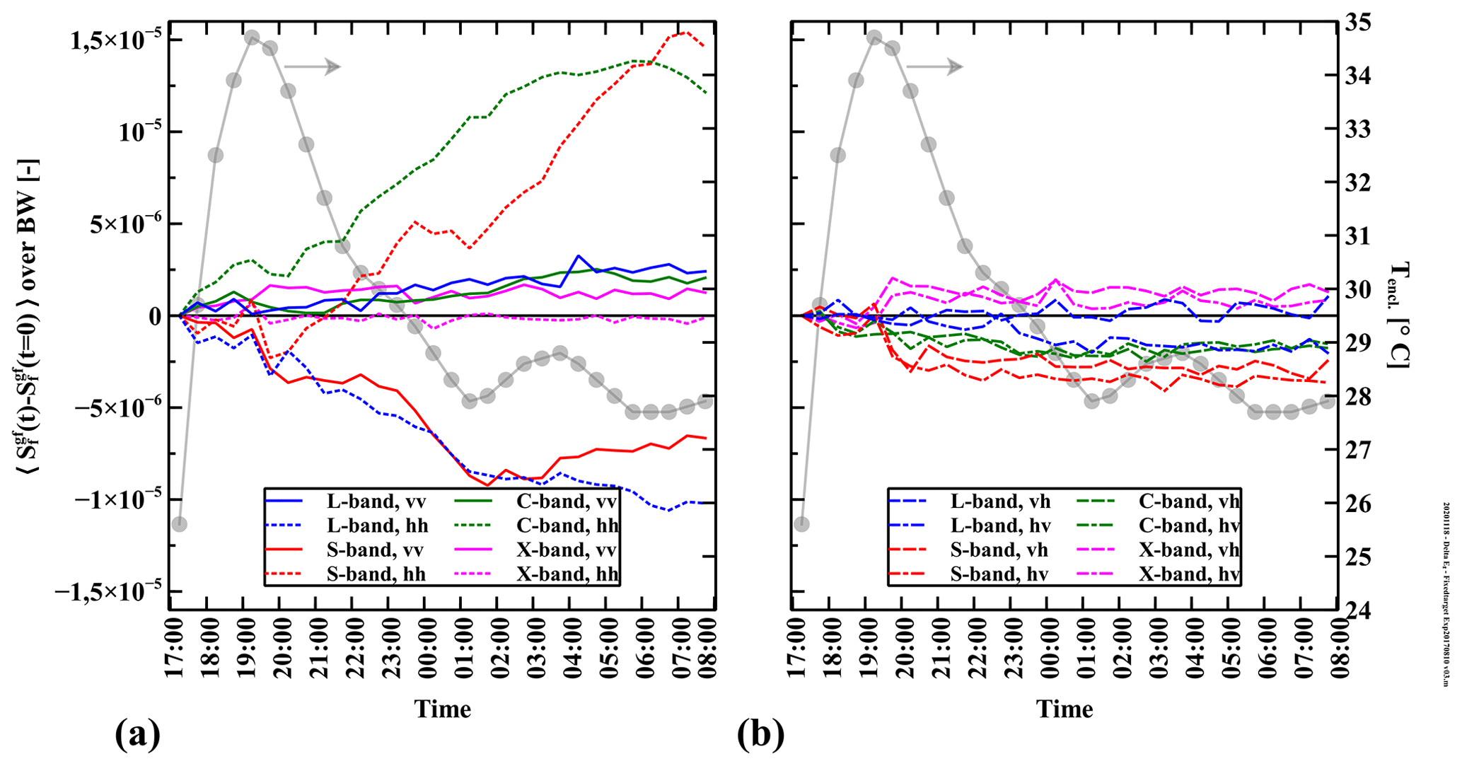
Figure E1Measured radar return from a fixed target over a varying enclosure temperature Tencl. Shown times are in local time.
For bandwidths at L-band (1.50–1.75 GHz), S-band (2.5–3.0 GHz), C-band (4.5–5.0 GHz), and X-band (9.0–9.9 GHz) the radar returns Ef (V m−1) (subscript f for “fixed target”) were filtered by a gate placed over the fixed target time-domain response, resulting in (superscript gf for “gate over fixed target”). The change in over time t, and thus over Tencl, is denoted :
In Fig. E1 the results of this experiment are shown. Plotted are the bandwidth-average difference of the S-parameter magnitudes over time (and temperature) with respect to the reference value , alongside Tencl. As explained in the main text, the quantities actually measured by the VNA were the S parameters, which are proportional to the corresponding values and .
There appeared to be no unique relationship between and Tencl. Within 3 h from the experiment start Tencl increases to a maximum value, after which it decreases again at an increasingly slowed rate. Also the curves , in general, change more rapidly over the first 5 h and then become more stable. However, the direction of change in Tencl – a rapid increase at the start followed by a fading decrease after 19:15 LT – is not seen in the curves. So in order to quantify the temperature-induced VNA instability we used the maximum observed variation of over time amidst all frequencies within BW to calculate the temperature-induced radar return uncertainty ΔST or, in the context of scattered electric-field strengths, its corresponding value ΔET (V m−1):
The quantity ΔET is to be treated as an absolute uncertainty of (Eq. C5) according to
with a factor two since both and are subject to this temperature-induced uncertainty. Table E1 lists the power levels at the VNA's receivers calculated from ΔST for the considered bandwidths and polarization channels.
E3 Reference target measurement uncertainty
E3.1 Reference target alignment
The absolute backscattering coefficient is determined with respect to the known RCS of a reference target. Errors in the used reference target RCS itself or errors made during the measurement of that target will contribute to the σ0 uncertainty. The RCS of a rectangular metal plate calculated with Eq. (B2) was found to match experimental observations fairly well (Ross, 1966), and therefore errors in the RCS of our rectangular plate itself were not considered. For the dihedral reflector we did the same, keeping in mind to only gate the specular reflection in the time domain and not also include the dihedral's edge reflections. As shown in Sorensen (1991) interference from diffraction of the dihedral's edges is not accounted for in Eq. (B2). We did consider errors in the measurement of the reference target; specifically we considered misalignment of the scatterometer's antennas towards the rectangular plate and vice versa.
The angular position of the reference targets with respect to the antenna boresight direction was estimated to be in the horizontal direction and in the vertical direction. Given the large distance from the antennas to the rectangular plate, R0=36.3 m, and the much smaller separation between the transmit and receive antennas, Want=0.4 m, single uncertainty values Δα0 and Δβ0 were used for both antennas. Due to this possible antenna misalignment the reference target is not illuminated by the peak value of the gain pattern, i.e. (–), resulting in an uncertainty in the measured radar response of the reference target and thus in K (W m−1). Equation (C3) then is modified to
The angular position of the individual antennas with respect to the reference target's surface normal (or frontal projection surface normal in case of the dihedral reflectors) was estimated with the help of a laser mounted between the two antennas and detachable mirrors on the reference targets. Optimal alignment was found by rotating the targets until the reflected laser spot was on (or close to) the laser aperture again. In the horizontal plane, the angle between the rectangular plate's surface normal and the transmit antenna was (right side of the normal) and for the receive antenna . In the vertical plane, the angle between the rectangular plate's surface normal and both antennas (as they are next to each other) was close to zero. We estimated the uncertainty of all aforementioned angles to be (both in the horizontal and vertical plane). For the small dihedral reflector these angles were in the horizontal and vertical plane, while for the large dihedral reflector and in the horizontal plane and in the vertical plane.
Starting with the physical optics model for the monostatic RCS of a metal rectangular plate, σ(θ,ϕ) (Kerr and Goldstein, 1951, p. 457), a crude bistatic-RCS version was created by simply imposing a linear phase delay along the plate's surface. We shall assume that this model will also hold for the dihedral reflector. Calculation of K can then be extended to include the (mis)alignment or offset of both individual antennas with respect to the reference targets and their uncertainties, which leads to Eq. (E4).
How the uncertainties Δα0, Δβ0, Δθi, and Δθs in Eq. (E4) propagate into the uncertainty of K, called the reference target measurement uncertainty ΔK, may be found in textbooks such as Hughes and Hase (2010). Resulting ΔK values, per considered BW and polarization, are presented as relative uncertainties in Table E1. With X-band the ΔK values are highest because the antenna radiation patterns are most narrow for higher frequencies.
E3.2 Validation reference target alignment
In this section we shall demonstrate that estimated values for the rotational offsets and uncertainties θi, θs, Δθi, and Δθs of the reference targets used are consistent with their respective measured radar returns. First we apply the radar equation (Eq. 1) to both the rectangular plate and the small dihedral reflector and substitute for PTX. We then have
where we dropped the polarization subscripts for readability. Since the values for α0 and β0 are the same for both measurements, the term containing the antenna gain patterns G is unity. We then end up with
Figure E2 shows the measured radar returns of the three calibration standards. For 5 GHz the difference between the small dihedral return and the rectangular plate for vv polarization is −3.3 dB. The term involving the distances R is −4.7 dB, resulting in the right side of Eq. (E6) being −8.0 dB. If both reference targets were perfectly aligned towards the antennas, the RCS ratio on the left side of Eq. (E6) would be −8.1 dB, which is 0.1 dB below the measured result. By finding suitable combinations of misalignment or offset angles θi and θs for both targets, Eq. (E6) can be satisfied. It can be shown that consistent angles can be found for all three reference targets which are within the ranges specified in Sect. E3.1. In the above procedure we used the co-polarization returns of the dihedral reflectors, while it is in fact the cross polarization that is of interest. We argue that the 45∘ rotation of the dihedral references – necessary for realizing the depolarization – does not introduce other significant angular offsets, and therefore the estimated values for the rotational offsets and uncertainties remain valid also for cross polarization. Note that the explained method cannot validate the angular positions of the reference targets with respect to the antenna boresight direction and their uncertainties – α0, Δα0 and β0, Δβ0 – as the term containing the antenna gain patterns was cancelled out.
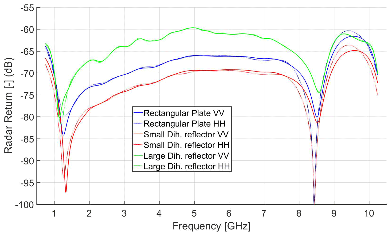
Figure E2Measured radar returns of calibration standards for co-polarization . Solid lines are VV, and dotted lines are HH polarization.
We conclude this section with some remarks on the features in the measured reference target return powers shown in Fig. E2. With all returns there is a sharp trough between 8–9 GHz, which is caused by a combination of a local increment of the antenna's return loss and an asymmetry in the antennas' E-plane radiation pattern between 7–9 GHz. The asymmetry causes the pattern's peaks to point off-target by about 10∘, resulting in a lower radar return. The deep troughs close to 1.3 GHz are caused by a combination of high return loss at the low-frequency edge of the antenna's operational bandwidth and an artefact of the gating procedure, which in this case lets rise at the edge. This gating artefact is known to distort the band edges of a gated frequency response (Keysight Technologies, 2020). To account for this artefact the bandwidths used for the ground surface measurements were broadened by 10 % at both edges prior to gating. The added edges were discarded again after gating. The curves of the rectangular plate and small dihedral reflector have a similar shape for most of the frequency band. Their difference is merely a constant factor as predicted by the physical optics model for RCS (Eq. B2). The curve shape of the large dihedral reflector however is clearly different from the other two. This is partly because of its more severe angular offsets θi and θs but also because the planar-wave condition is not met for most of the frequency band; see Table B1.
E4 Antenna coupling remnant
Because the transmit and receive antennas are placed next to each other in order to measure the monostatic σ0, part of the transmitted signal leaks, or couples, directly into the receive antenna, thereby interfering with the target return of interest. This antenna coupling is strongest for the lower frequencies (L-band) because these have the broadest antenna radiation patterns (see Fig. B3). With respect to the polarization channels, the antenna coupling is strongest for hh because of how the electric-field lines of the principal TE10 modes, in the particular case of hh polarization, couple strongest when the antenna apertures are next to each other. With the cross-polarization channels the coupling is weakest because of how the principal field components are perpendicular between the transmit and receive antenna.
Although the majority of the antenna coupling can be filtered out by gating, a remnant remains present in the filtered frequency domain response. This becomes apparent when the antennas are pointed skywards and the time-domain response is calculated per BW. Between the times and distances and , where, during measurement of the ground target, the scattering events of interest are located, the signal is not yet at its lowest level beyond 10 m. This effect is strongest for the L-band BW with hh polarization, while for X-band the time-domain response level between rsg and reg is almost equal to its lowest level.
From the sky measurement the coupling remnant was retrieved. When measuring the ground surface, the antenna coupling process of course interferes with the ground return. However, because we measure over a bandwidth and the ground return is a randomly fluctuating signal, we argue that , so the average over BW can simply be subtracted from the (gated) ground return .
E5 Propagation of uncertainties
In this section we demonstrate how Eq. (4) is derived. We show, using error propagation theory, how each of the (three) error terms, ΔET, ΔK, and fading, propagates into an error for σ0 and how all errors may be combined into one statistical confidence interval for σ0. We start with Eq. (C1), which with Eq. (C4) can be written as
The term between brackets in the denominator we may simply rewrite as F±ΔF, i.e. a variable with an error. The variables IN and K also have their respective errors ΔIN and ΔK. When we write all variables and their errors explicitly we end up with
We shall now describe all three error terms, starting with ΔIN. The calculation of IN from the measured backscattered electric field is given by Eq. (E3) as
with ΔET as measurement uncertainty. As explained in Sect. C2, every term in the above sum may be considered an independent variable. Because the number of samples N within BW is sufficiently large (about 15), we consider ΔET as a statistical error and therefore use the corresponding equation for error propagation (see for example Hughes and Hase, 2010) to calculate the total statistical error ΔIN:
ΔIN can be considered the 1-standard-deviation value of IN. Since the number of terms in the sum N are large enough, we can consider ±ΔIN as the edges of a 66 % confidence interval for IN.
As explained in Sect. E3.1, ΔK can be calculated by using error propagation theory for the errors Δα0, Δβ0, and those associated with the bistatic RCS of the rectangular metal plate and dihedral reflectors Δθi and Δθs. Note, however, that these are maximum possible errors so that the corresponding error propagation rules should be used. In order to have differentiable functions for the E-plane and H-plane antenna gain patterns, Epatt(α0) and Hpatt(β0) respectively, the measured radiation patterns can be fitted with Gaussian functions for angles close to antenna boresight. Writing ΔK explicitly is then straightforward.
Finally, we have the error term ΔF, which is equal to . As explained in Sect. C1 this error represents a 68 % confidence interval for .
Returning to Eq. (E8) we now combine all three errors into one statistical error. To do so we must first convert ΔK from being a maximum possible error into a statistical error like ΔIN and ΔF. This can be done by multiplying ΔK with , so the result may be interpreted as a 1-standard-deviation value for K. This is equivalent to saying that is a 68 % confidence interval for K. We combine the three statistical errors conservatively into a 66 % confidence interval for σ0:
where Δσ0 is calculated according to the error propagation equation for statistical errors:
We start with the asphalt experiment results, which we present here to demonstrate that our σ0 retrieval method, using measurement data obtained with our scatterometer system, results in σ0 values comparable to those in other studies.
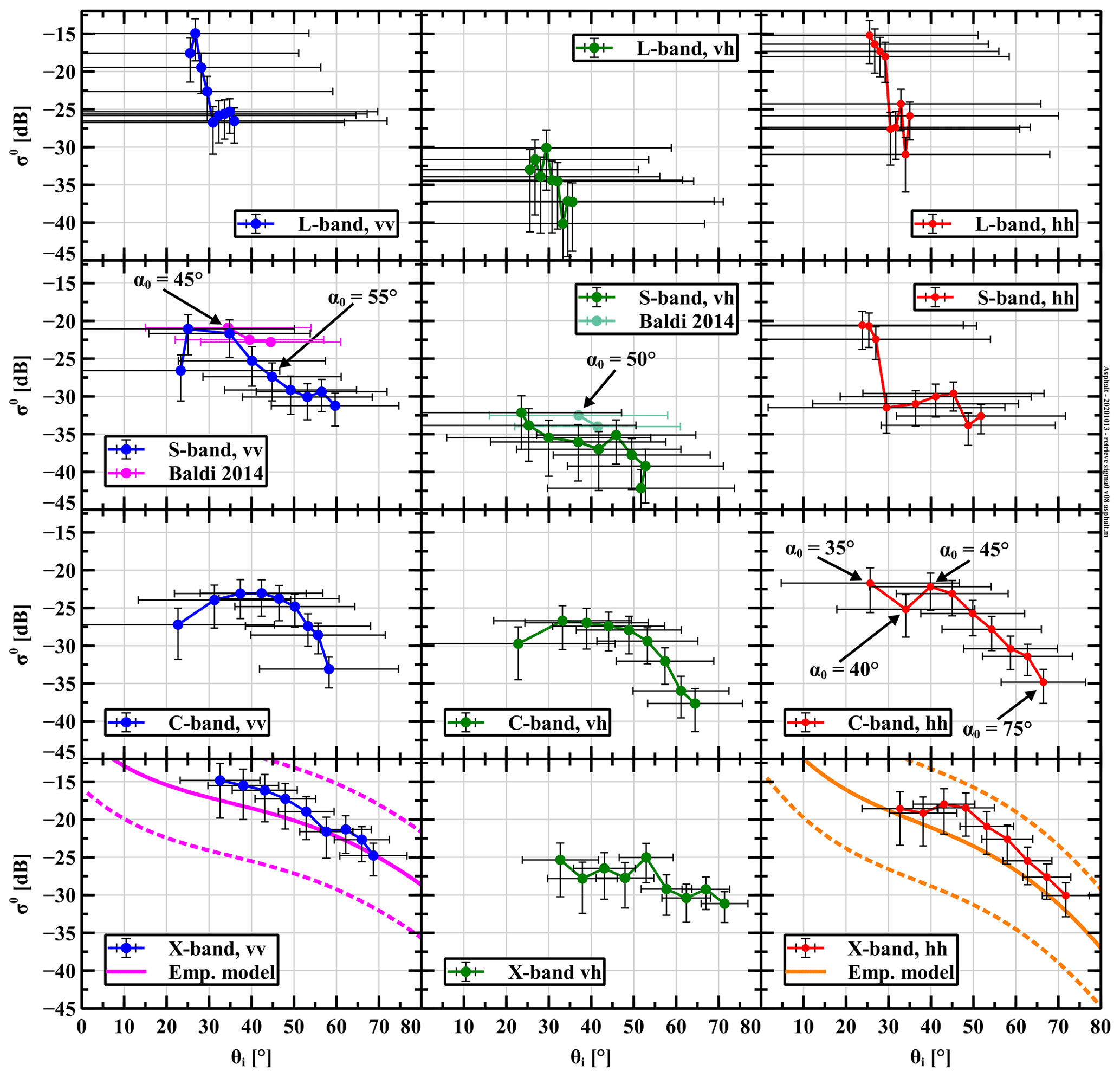
Figure F1Measurement results of for all bands and polarizations together with S-band measurement results from Baldi (2014) and empirical model for X-band from Ulaby and Dobson (1989). Points represent results for different antenna boresight angles α0. Horizontal bars represent intervals for angle of incidence θ, and vertical bars represent the 66 % confidence interval for σ0. Dotted lines between data points serve as guides. With X-band, solid and dotted curves (magenta and orange) represent the mean value and 90 % confidence interval of the empirical model respectively.
Figure F1 shows our retrieved over α0 for all bandwidths and polarization channels. Since with all bands the uncertainty intervals for vh and hv overlap, we only show the vh cross-polarization channel for figure clarity. When comparing the results for S-, C-, and X-band we observe an increase in backscatter over frequency, which can be explained by the increment of the surface-roughness-to-wavelength ratio. For X- and C-band the vv backscatter is stronger than with hh. For S-band this also holds, although the comparison is more difficult as the θ intervals become broader. It is clear, however, that for all bands the cross response is lower than that of the co-polarization. Remarkable, at first sight, is the fact that the retrieved σ0 for L-band is higher than that of S-band. We believe this is due to the lowest angular resolution of our system at L-band and our subsequent σ0 retrieval method from the measured signal. As shown in the graphs, for L-band the backscatter from near-nadir θ angles is included in the received signal for almost all α0 angular positions. As the actual σ0(θ), in general, shoots upward for the smaller θ angles towards the peak value at nadir, the resulting signal, and with it the retrieved σ0, is high as well.
Our results are plotted together with those found in other studies. Baldi (2014) also measured asphalt backscatter for S-band. His scatterometer had a more narrow beamwidth of 10∘, allowing for a straightforward measurement of σ0 over θ. He measured over . For a comparison to our results, we used his measured σ0(θ) in Eq. (2) and subsequently applied our retrieval method to this simulated radar return PRX. The resulting σ0 values are shown in Fig. F1. Three points for vv polarization and two for vh polarization could be retrieved. Because no data were presented outside the 15–55∘ range the hh polarization response could not be simulated. In general, we consider our results to match with Baldi's satisfactorily. The differences may be attributed to fading uncertainty (low number of spatial samples) and to different surface roughness values: it seems our asphalt was smoother. However, the latter argument is speculative since neither we nor Baldi measured the surface roughness.
The only other study on L-band backscatter from asphalt we could find was that by Peake and Oliver (1971). There σ0 values are reported for smooth asphalt with an estimated surface roughness of s=0.3 mm for for vv and for hh. Because of the broad L-band θ ranges for our scatterometer, however, a simulation of the σ0 retrieval, as with Baldi's data, would be incorrect.
For X-band with co-polarization we compare our results with the empirical model for asphalt described in Ulaby and Dobson (1989). This model is formed using measurements from multiple other studies with asphalt having various roughness values. Since our antenna beamwidths at X-band are sufficiently narrow, we can compare our results without further adjustment. No empirical model is given for asphalt at X-band with cross polarization in Ulaby and Dobson (1989). For both vv and hh polarization our retrieved σ0 shows a clear overall decreasing trend over θ, which is expected for a surface that is smooth compared to the wavelength. Overall, σ0 for vv polarization is higher than for hh polarization, which is in accordance to the empirical model. Starting from the smaller angles, the consecutive measurement points remain at similar level. With hh polarization there appears to be even a local minimum at 40∘, although the measurement uncertainty is relatively large there. Given that the empirical curves show a similar trend, though not as pronounced, the slow decay of over θ for 25–55∘ can simply be a property of asphalt. Overall we find our measurements to lie within the 90 % occurrence interval of the empirical model and therefore conclude that our results for asphalt are similar to those of Ulaby and Dobson (1989). We could not find studies reporting asphalt backscatter for C-band.
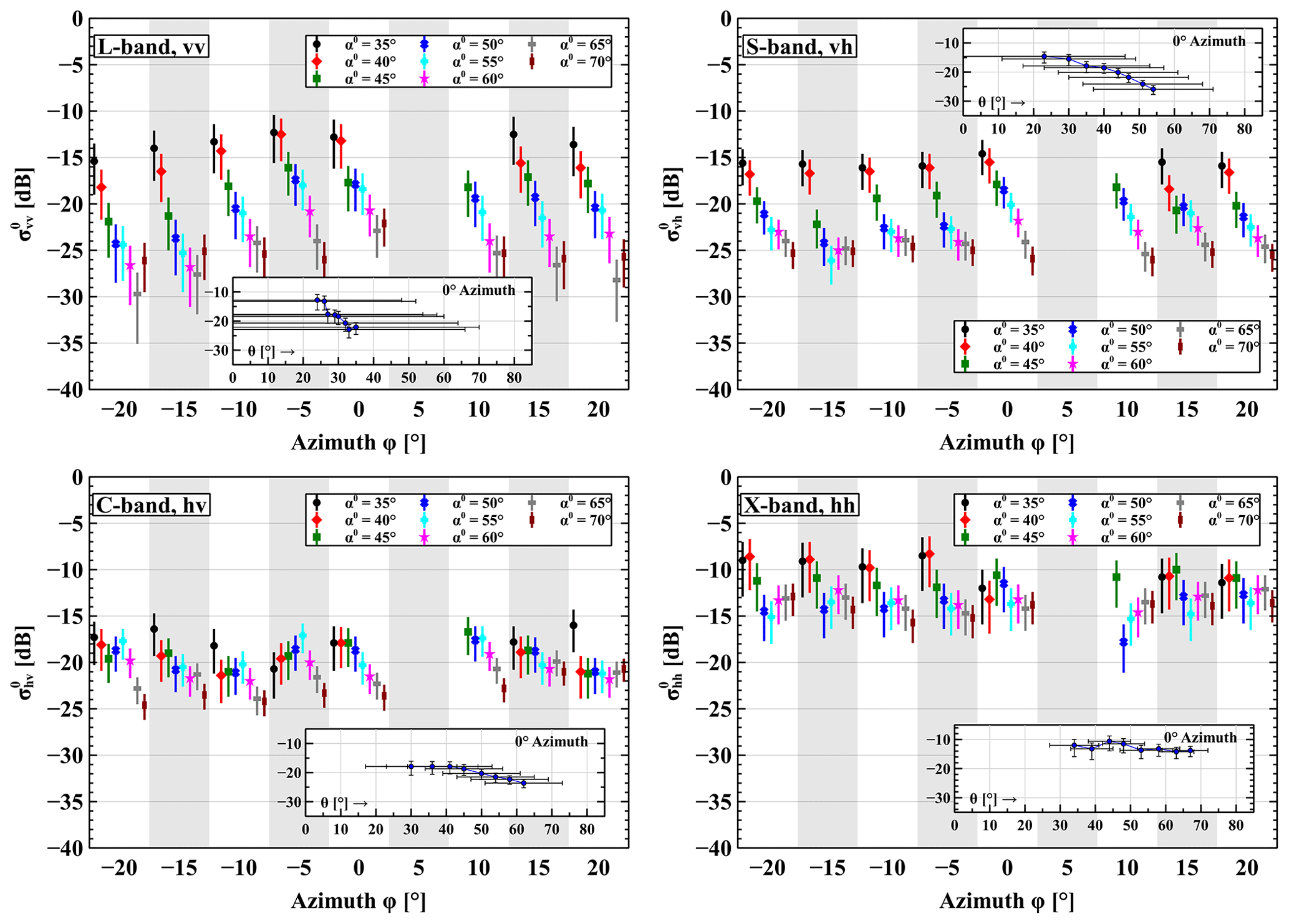
Figure G1Measurement of for all bandwidths at different polarization over the Maqu site on 25 August 2017. Four main figures: for different antenna boresight azimuth angles ϕ, the variation of over boresight elevation angles α0 is shown. The eight vertical bars represent the 66 % confidence interval for σ0. Intervals for incidence angles θ per measurement are not shown here for figure clarity. Insets: for . Horizontal bars represent intervals of actual incidence angles θ, which are identical for other ϕ values in the main figures.
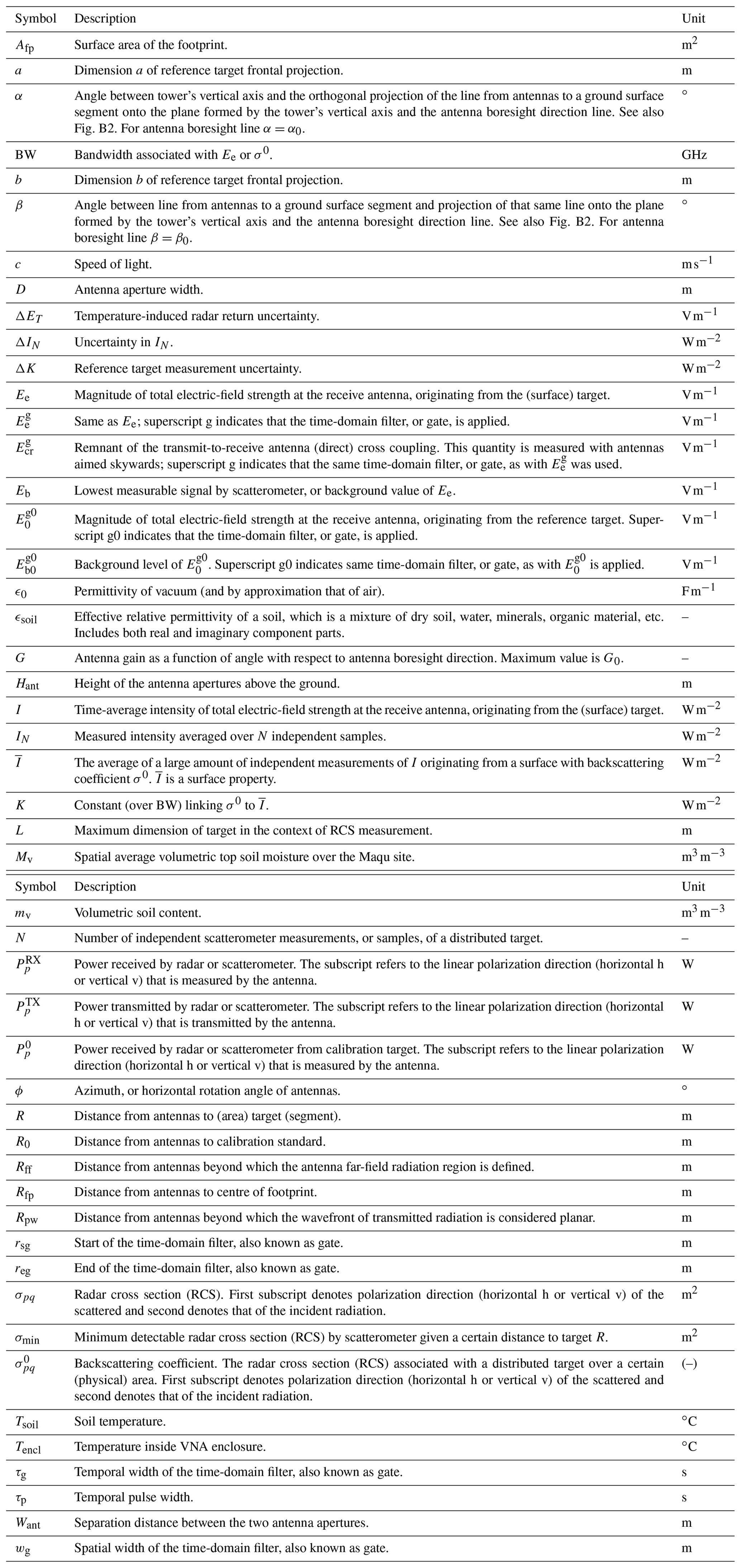
JGH wrote this paper, installed and operated the scatterometer system, developed the data processing and σ0 retrieval process, and performed the data analysis. RvdV advised in the experiment designs, σ0 retrieval process, and paper structure. XW, ZW, and DZ handled the China customs logistics and installed and operated the scatterometer system. On a regular basis they maintained the scatterometer system and the Maqu site. CvdT advised in the σ0 retrieval process. JW and ZS conceptualized the experiment design. All co-authors commented on and revised the paper.
The authors declare that they have no conflict of interest.
This research has been supported in part by the ESA ELBARA-II/III loan agreement (grant no. EOP-SM/2895/TC-tc), the ESA MOST Dragon IV Program (Monitoring Water and Energy Cycles at Climate Scale in the Third Pole Environment), the Netherlands Organization for Scientific Research (project no. ALW-GO/14-29), the National Natural Science Foundation of China (grant no. 41971033), and the Fundamental Research Funds for the Central Universities, CHD (grant no. 300102298307).
This paper was edited by Birgit Heim and reviewed by two anonymous referees.
Axline, R. M.: Experimental and Simulated Study of Scattering from Randomly Rough Surfaces, Phd thesis, University of Kansas, Lawrence, Arkansas, USA, 1974. a
Balanis, C. A.: Antenna Theory: Analysis and Design, 3rd edn., Wiley Interscience, Hoboken, NJ, USA, 2005. a
Baldi, C. A.: The Design, Validation and Analysis of Surface Based S-band and D-band Polarimetric Scatterometers, Msc thesis, University of Massachusetts Amherst, MA, USA, 2014. a, b, c, d, e
Bansal, R.: The Far-Field; how far is far enough?, Applied Microwave and Wireless, 11, 59–60, 1999. a
Clapp, R. E.: A Theoretical and Experimental Study of Radar Ground Return, Report 1024, Massachusetts Institute of Technology, Cambridge, Massachusetts, USA, 1946. a
Dente, L., Ferrazzoli, P., Su, Z., van der Velde, R., and Guerriero, L.: Combined use of Active and Passive Microwave Satellite Data to constrain a Discrete Scattering Model, Remote Sens. Environ., 155, https://doi.org/10.1016/j.rse.2014.08.031, 2014. a, b
De Porrata-Dória i Yagüe, R., Ibars, A. B., and Martínez, L. F.: Analysis and Reduction of the Distortions induced by Time-Domain filtering techniques in Network Analyzers, IEEE T. Instrum. Meas., 47, 930–934, https://doi.org/10.1109/19.744645, 1998. a
de Roo, R. D. and Ulaby, F. T.: Bistatic Specular Scattering from Rough Dielectric Surfaces, IEEE T. Antenn. Propag., 42, 220–231, https://doi.org/10.1109/8.277216, 1994. a
Dobson, M. C., Ulaby, F. T., Hallikainen, M. T., and El-rayes, M. A.: Microwave Dielectric Behavior of Wet Soil-Part II: Dielectric Mixing Models, IEEE T. Geosci. Remote, GE-23, 35–46, https://doi.org/10.1109/TGRS.1985.289498, 1985. a, b
Famiglietti, J. S., Ryu, D., Berg, A. A., Rodell, M., and Jackson, T. J.: Field Observations of Soil Moisture Variability across Scales, Water Resour. Res., 44, W01423, https://doi.org/10.1029/2006wr005804, 2008. a
Fung, A. K., Liu, W. Y., Chen, K. S., and Tsay, M. K.: An Improved Iem Model for Bistatic Scattering From Rough Surfaces, J. Electromagnet. Wave., 16, 689–702, https://doi.org/10.1163/156939302X01119, 2002. a, b
Geldsetzer, T., Mead, J. B., Yackel, J. J., Scharien, R. K., and Howell, S. E. L.: Surface-Based Polarimetric C-Band Scatterometer for Field Measurements of Sea Ice, IEEE T. Geosci. Remote, 45, 3405–3416, https://doi.org/10.1109/TGRS.2007.907043, 2007. a
He, Y., Guo, X., and Wilmshurst, J. F.: Comparison of Different Methods for measuring Leaf Area Index in a Mixed Grassland, Can. J. Plant Sci., 87, 803–813, https://doi.org/10.4141/CJPS07024, 2007. a
Hofste, J., van der Velde, R., Wang, X., Zheng, D., Wen, J., van der Tol, C., and Su, Z.: Broadband Full Polarimetric Scatterometry for Monitoring Soil Moisture and Vegetation Properties Over a Tibetan Meadow, in: IGARSS 2018 – 2018 IEEE International Geoscience and Remote Sensing Symposium, 22–27 July 2018, Valencia, Spain, 2007–2010, Hofste2018, https://doi.org/10.1109/IGARSS.2018.8519380, 2018. a
Hofste, J. G.: Matlab Source Code for retrieving Backscatter Coefficients, Data Archiving and Networked Services (DANS) [code], https://doi.org/10.17026/dans-xyf-fmkk, 2021. a, b
Hofste, J. G., van der Velde, R., Wen, J., Wang, X., Wang, Z., Zheng, D., and Su, Z.: Long-term Ground-based Broadband Microwave Scatterometer Observations of an Alpine Meadow over the Tibetan Plateau, Data Archiving and Networked Services (DANS) [data set], https://doi.org/10.17026/dans-zfb-qegy, 2021. a, b, c
Hughes, I. and Hase, T.: Measurements and their Uncertainties : a Practical Guide to Modern Error Analysis, Oxford University Press, Oxford, UK, 2010. a, b, c
Hwang, J., Kwon, S., and Oh, Y.: Evaluation of Calibration Accuracy with HPS (Hongik Polarimetric Scatterometer) Aystem for Multi-Bands and Multi-Polarizations, in: IGARS 2011–2011 IEEE International Geoscience and Remote Sensing Symposium, 24–29 July 2011, Vancouver, BC, Canada, 3987–3990, https://doi.org/10.1109/IGARSS.2011.6050105, 2011. a
Jersak, B. D., Dolaty, M., and Blanchard, A. J.: Time Domain Enhancement of Frequency Domain Radar Cross-Section Data, Int. J. Remote Sens., 13, 2105–2119, https://doi.org/10.1080/01431169208904256, 1992. a
Joseph, A. T., van der Velde, R., O'Neill, P. E., Lang, R., and Gish, T.: Effects of Corn on C- and L-band Radar Backscatter: A Correction Method for Soil Moisture Retrieval, Remote Sens. Environ., 114, 2417–2430, https://doi.org/10.1016/j.rse.2010.05.017, 2010. a
Kerr, D. E. and Goldstein, H.: Radar Targets and Echoes, in: Propagation of Short Radio Waves, edited by: Kerr, D. E., McGraw-Hill Book Company Inc., New York, USA, 445–587, 1951. a, b
Keysight Technologies: PNA Receiver Reduces Antenna RCS measurement Test Times, 5989-1949EN, available at: http://www.keysight.com (last access: 15 June 2021), 2017. a, b
Keysight Technologies: Keysight 2-port and 4-port PNA-L Network Analyzer, 9018-04407, available at: http://www.keysight.com (last access: 15 June 2021), 2018. a
Keysight Technologies: Time Domain Analysis Using a Network Analyzer, 7018-01451, available at: http://www.keysight.com (last access: 15 June 2021), 2020. a
Kim, Y., Jackson, T., Bindlish, R., Hong, S., Jung, G., and Lee, K.: Retrieval of Wheat Growth Parameters With Radar Vegetation Indices, IEEE Geosci. Remote S., 11, 808–812, https://doi.org/10.1109/LGRS.2013.2279255, 2014. a, b
Kouyoumjian, R. G. and Peters, L.: Range Requirements in Radar Cross-Section Measurements, P. IEEE, 53, 920–928, https://doi.org/10.1109/PROC.1965.4070, 1965. a
Kweon, S. and Oh, Y.: A Modified Water-Cloud Model With Leaf Angle Parameters for Microwave Backscattering From Agricultural Fields, IEEE T. Geosci. Remote, 53, 2802–2809, https://doi.org/10.1109/TGRS.2014.2364914, 2015. a
Lin, C., Rommen, B., Floury, N., Schüttemeyer, D., Davidson, M. W. J., Kern, M., Kontu, A., Lemmetyinen, J., Pulliainen, J., Wiesmann, A., Werner, C., Mätzler, C., Schneebeli, M., Proksch, M., and Nagler, T.: Active Microwave Scattering Signature of Snowpack – Continuous Multiyear SnowScat Observation Experiments, IEEE J. Sel. Top. Appl., 9, 3849–3869, https://doi.org/10.1109/JSTARS.2016.2560168, 2016. a, b
Liu, P.-W., Judge, J., DeRoo, R. D., England, A. W., Bongiovanni, T., and Luke, A.: Dominant Backscattering Mechanisms at L-band during Dynamic Soil Moisture Conditions for Sandy Soils, Remote Sens. Environ., 178, 104–112, https://doi.org/10.1016/j.rse.2016.02.062, 2016. a
Lv, S., Zeng, Y., Wen, J., Zhao, H., and Su, Z.: Estimation of Penetration Depth from Soil Effective Temperature in Microwave Radiometry, Remote Sens., 10, 519, https://doi.org/10.3390/rs10040519, 2018. a
MacArthur, A., Robinson, I., Rossini, M., Davis, N., and MacDonald, K.: A Dual-Field-of-View Spectrometer System for Reflectance and Fluorescence Measurements (Piccolo Doppio) and Correction of Etaloning, in: Fifth International Workshop on Remote Sensing of Vegetation Fluorescence, 22–24 April 2014, Paris, France, European Space Agency, 2014. a
Mätzler, C.: Applications of the interaction of microwaves with the natural snow cover, Remote Sensing Reviews, 2, 259–387, https://doi.org/10.1080/02757258709532086, 1987. a
Miller, D. J.: The Tibetan Steppe, in: Grasslands of the world, edited by: Suttie, J. M., Reynolds, S. G., and Batello, C., Food and Agricultural Organization of the United Nations, Rome, Italy, available at: ftp://ftp.fao.org/docrep/fao/008/y8344e/y8344e00.pdf (last access: 11 June 2021), 2005. a, b
Monakov, A. A., Vivekanandan, J., Stjernman, A. S., and Nystrom, A. K.: Spatial and frequency averaging techniques for a polarimetric scatterometer system, IEEE T. Geosci. Remote, 32, 187–196, https://doi.org/10.1109/36.285201, 1994. a
Nagarajan, K., Liu, P. W., De Roo, R., Judge, J., Akbar, R., Rush, P., Feagle, S., Preston, D., and Terwilleger, R.: Automated L-Band Radar System for Sensing Soil Moisture at High Temporal Resolution, IEEE Geosci. Remote S., 11, 504–508, https://doi.org/10.1109/LGRS.2013.2270453, 2014. a, b, c, d
Nandan, V., Geldsetzer, T., Islam, T., Yackel, J. J., Gill, J. P. S., Fuller, M. C., Gunn, G., and Duguay, C.: Ku-, X- and C-band Measured and Modeled Microwave Backscatter from a Highly Saline Snow Cover on First-year Sea Ice, Remote Sens. Environ., 187, 62–75, https://doi.org/10.1016/j.rse.2016.10.004, 2016. a, b
Nesti, G. and Hohmann, M.: An Efficient Calibration Procedure For Polarimetric Radar Systems, in: IGARSS 1990–1990 IEEE International Geoscience and Remote Sensing Symposium, 20–24 May 1990, College Park, MD, USA, 1099–1103, https://doi.org/10.1109/IGARSS.1990.688685, 1990. a, b
Oh, Y., Sarabandi, K., and Ulaby, F. T.: An Empirical Model and an Inversion Technique for Radar Scattering from Bare Soil Surfaces, IEEE T. Geosci. Remote, 30, 370–381, https://doi.org/10.1109/36.134086, 1992. a
Peake, W. and Oliver, T. L.: The Response of Terrestrial Surfaces at Microwave Frequencies, Report 2440-7, Ohio State University, ElectroScience Laboratory, Columbus, Ohio, USA, 1971. a
Peel, M. C., Finlayson, B. L., and McMahon, T. A.: Updated world map of the Köppen-Geiger climate classification, Hydrol. Earth Syst. Sci., 11, 1633–1644, https://doi.org/10.5194/hess-11-1633-2007, 2007. a
Ross, R.: Radar Cross Section of Rectangular Flat Plates as a Function of Aspect Angle, IEEE T. Antenn. Propag., 14, 329–335, https://doi.org/10.1109/TAP.1966.1138696, 1966. a
Schwank, M., Wiesmann, A., Werner, C., Mätzler, C., Weber, D., Murk, A., Völksch, I., and Wegmüller, U.: ELBARA II, an L-Band Radiometer System for Soil Moisture Research, Sensors, 10, 584–612, 2010. a, b
Schwarzbeck Mess-Elektronic OHG: Radiation Patterns BBHX 9120 LF Antenna, available at: http://www.schwarzbeck.de (last access: 11 June 2021), 2017. a, b, c
Seneviratne, S. I., Corti, T., Davin, E. L., Hirschi, M., Jaeger, E. B., Lehner, I., Orlowsky, B., and Teuling, A. J.: Investigating Soil Moisture–Climate Interactions in a Changing Climate: A Review, Earth-Sci. Rev., 99, 125–161, https://doi.org/10.1016/j.earscirev.2010.02.004, 2010. a
Skolnik, M.: Radar Handbook, 3rd edn., McGraw-Hill, New York, USA, 2008. a
Sorensen, K. W.: A Dihedral Corner Reflector Model for Full Polarization Calibration of RCS Measurements, in: Antennas and Propagation Society Symposium 1991 Digest, 20–24 June 1991, London, ON, Canada, vol. 2, 748–751, https://doi.org/10.1109/APS.1991.174947, 1991. a
Stiles, J. M., Sarabandi, K., and Ulaby, F. T.: Electromagnetic Scattering from Grassland-Part II: Measurement and Modeling Results, IEEE T. Geosci. Remote, 38, 349–356, https://doi.org/10.1109/36.823930, 2000. a
Su, Z., de Rosnay, P., Wen, J., Wang, L., and Zeng, Y.: Evaluation of ECMWF's Soil Moisture Analyses using Observations on the Tibetan Plateau, J. Geophys. Res.-Atmos., 118, 5304–5318, https://doi.org/10.1002/jgrd.50468, 2013. a
Su, Z., Wen, J., Zeng, Y., Zhao, H., Lv, S., van der Velde, R., Zheng, D., Wang, X., Wang, Z., Schwank, M., Kerr, Y., Yueh, S., Colliander, A., Qian, H., Drusch, M., and Mecklenburg, S.: Multiyear In-Situ L-band Microwave Radiometry of Land Surface Processes on the Tibetan Plateau, Scientific Data, 7, 317, https://doi.org/10.1038/s41597-020-00657-1, 2020. a, b
Tan, L. and Jiang, J.: Digital Signal Processing, Fundamentals and Applications, 2nd edn., Academic Press, Waltham, MA, USA, 2013. a
Ulaby, F. T. and Long, D. G.: Microwave Radar and Radiometric Remote Sensing, 4th edn., The University of Michigan Press, Ann Arbor, USA, 2017. a, b, c, d
Ulaby, F. T., Moore, R. K., and Fung, A. K.: Microwave Remote Sensing Active and Passive Vol. II: Radar Remote Sensing and Surface Scattering and Emission Theory, Addison-Wesley Publishing Company, Reading, Massachusetts, USA, 1982. a, b
Ulaby, F. T., Allen, C. T., and Fung, A. K.: Method for Retrieving the True Backscattering Coefficient from Measurements with a Real Antenna, IEEE T. Geosci. Remote, GE-21, 308–313, https://doi.org/10.1109/TGRS.1983.350558, 1983. a
Ulaby, F. T., Haddock, T. F., and Austin, R. T.: Fluctuation Statistics of Millimeter-Wave Scattering from Distributed Targets, IEEE T. Geosci. Remote, 26, 268–281, https://doi.org/10.1109/36.3030, 1988. a, b, c, d
Ulaby, F. W. and Dobson, M. C.: Handbook of Radar Scattering Statistics for Terrain, Artech House Inc., Norwood, MA, USA, 1989. a, b, c, d, e, f, g
Vachaud, G., Passerat De Silans, A., Balabanis, P., and Vauclin, M.: Temporal Stability of Spatially Measured Soil Water Probability Density Function, Soil Sci. Soc. Am. J., 49, 822–828, https://doi.org/10.2136/sssaj1985.03615995004900040006x, 1985. a
Wang, Q. and Gogineni, S.: A Numerical Procedure for Recovering Scattering Coefficients from Measurements with Wide-Beam Antennas, IEEE T. Geosci. Remote, 29, 778–783, https://doi.org/10.1109/36.83993, 1991. a
Wang, Q., van der Velde, R., Su, Z., and Wen, J.: Aquarius L-band Scatterometer and Radiometer Observations over a Tibetan Plateau Site, Int. J. Appl. Earth Obs., 45, 165–177, https://doi.org/10.1016/j.jag.2015.06.010, 2016. a
Werner, C., Wiesmann, A., Strozzi, T., Schneebeli, M., and Mätzler, C.: The Snowscat Ground-Based Polarimetric Scatterometer: Calibration and Initial Measurements from Davos Switzerland, in: 2010 IEEE International Geoscience and Remote Sensing Symposium, 25–30 July 2010, Honolulu, HI, USA, 2363–2366, Werner2010, https://doi.org/10.1109/IGARSS.2010.5649015, 2010. a, b
Zheng, D., van der Velde, R., Su, Z., Wen, J., Wang, X., and Yang, K.: Evaluation of Noah Frozen Soil Parameterization for Application to a Tibetan Meadow Ecosystem, J. Hydrometeorol., 18, 1749–1763, https://doi.org/10.1175/jhm-d-16-0199.1, 2017a. a, b
Zheng, D., Wang, X., Velde, R. v. d., Zeng, Y., Wen, J., Wang, Z., Schwank, M., Ferrazzoli, P., and Su, Z.: L-Band Microwave Emission of Soil Freeze–Thaw Process in the Third Pole Environment, IEEE T. Geosci. Remote, 55, 5324–5338, https://doi.org/10.1109/TGRS.2017.2705248, 2017b. a, b, c, d
Zheng, D., Li, X., Wang, X., Wang, Z., Wen, J., van der Velde, R., Schwank, M., and Su, Z.: Sampling Depth of L-band Radiometer Measurements of Soil Moisture and Freeze-Thaw Dynamics on the Tibetan Plateau, Remote Sens. Environ., 226, 16–25, https://doi.org/10.1016/j.rse.2019.03.029, 2019. a, b
In reality the measured fields or signals remain complex until after the gating process. We, however, stick to this terminology for clarity.
Not to be confused with the scattering amplitudes used in scattering theory, which have units of metres (m); see for example Ulaby and Long (2017).
- Abstract
- Introduction
- Study region and climate
- Methodology
- Measurement results
- Discussion
- Code and data availability
- Conclusions
- Appendix A: Results supporting measurements
- Appendix B: Technical details scatterometer
- Appendix C: Technical details σ0 retrieval procedure
- Appendix D: Three 13 d time series of σ0
- Appendix E: Details on sources of measurement uncertainty
- Appendix F: Angular variation of for asphalt
- Appendix G: Examples of over α0 for Maqu
- Appendix H
- Author contributions
- Competing interests
- Financial support
- Review statement
- References