Coastal Ocean Data Analysis Product in North America (CODAP-NA) – an internally consistent data product for discrete inorganic carbon, oxygen, and nutrients on the North American ocean margins

Internally consistent, quality-controlled (QC) data products play an important role in promoting regional-to-global research efforts to understand societal vulnerabilities to ocean acidification (OA). However, there are currently no such data products for the coastal ocean, where most of the OA-susceptible commercial and recreational fisheries and aquaculture industries are located. In this collaborative effort, we compiled, quality-controlled, and synthesized 2 decades of discrete measurements of inorganic carbon system parameters, oxygen, and nutrient chemistry data from the North American continental shelves to generate a data product called the Coastal Ocean Data Analysis Product in North America (CODAP-NA). There are few deep-water (> 1500 m) sampling locations in the current data product. As a result, crossover analyses, which rely on comparisons between measurements on different cruises in the stable deep ocean, could not form the basis for cruise-to-cruise adjustments. For this reason, care was taken in the selection of data sets to include in this initial release of CODAP-NA, and only data sets from laboratories with known quality assurance practices were included. New consistency checks and outlier detections were used to QC the data. Future releases of this CODAP-NA product will use this core data product as the basis for cruise-to-cruise comparisons. We worked closely with the investigators who collected and measured these data during the QC process. This version (v2021) of the CODAP-NA is comprised of 3391 oceanographic profiles from 61 research cruises covering all continental shelves of North America, from Alaska to Mexico in the west and from Canada to the Caribbean in the east. Data for 14 variables (temperature; salinity; dissolved oxygen content; dissolved inorganic carbon content; total alkalinity; pH on total scale; carbonate ion content; fugacity of carbon dioxide; and substance contents of silicate, phosphate, nitrate, nitrite, nitrate plus nitrite, and ammonium) have been subjected to extensive QC. CODAP-NA is available as a merged data product (Excel, CSV, MATLAB, and NetCDF; https://doi.org/10.25921/531n-c230, https://www.ncei.noaa.gov/data/oceans/ncei/ocads/metadata/0219960.html, last access: 15 May 2021) (Jiang et al., 2021a). The original cruise data have also been updated with data providers' consent and summarized in a table with links to NOAA's National Centers for Environmental Information (NCEI) archives (https://www.ncei.noaa.gov/access/ocean-acidification-data-stewardship-oads/synthesis/NAcruises.html).

1 Introduction

Anthropogenic ocean acidification (OA) refers to the process by which the ocean's uptake of excess anthropogenic atmospheric carbon dioxide (CO₂) reduces ocean pH and calcium carbonate mineral saturation states (Feely et al., 2004; Orr et al., 2005; Jiang et al., 2019; IPCC, 2011). OA is making it more difficult for marine calcifiers to build shells and skeletal structures and is endangering coral reefs and other marine ecosystems (Gattuso and Hanson, 2011; Doney et al., 2020). Coastal ecosystems account for most of the economic activities related to commercial and recreational fisheries and aquaculture industries, supporting about 90 % of the global fisheries yield and 80 % of known species of marine fish (Cicin-Sain et al., 2002). Studies have shown that OA has the potential to significantly impact both the fisheries and aquaculture industries and change the way humans make their living, run their communities, and live their lives in coastal regions around the world (Cooley and Doney, 2009; Barton et al., 2012, 2015).

The Global Ocean Data Analysis Project (GLODAPv2) offers an internally consistent data product for discrete-sampling-based open-ocean carbonate chemistry, nutrient chemistry, isotope, and transient tracer data (Olsen et al., 2016, 2020), allowing for a slew of new research products related to OA and its temporal trends in the global ocean (e.g., Lauvset et al., 2015; Jiang et al., 2015a; Gruber et al., 2019; Lauvset et al., 2020). While there are several data products and climatologies for coastal surface water partial pressure of CO₂ (pCO₂) (e.g., Bakker et al., 2016; Laruelle et al., 2017; Roobaert et al., 2019; Takahashi et al., 2020), internally consistent data products for water column carbonate and nutrient chemistry data in the coastal ocean currently do not exist. Such products would contribute significantly to our understanding of the current status of OA and its temporal trends and help guide OA mitigation and adaptation efforts in coastal oceans.

The impact of OA on North American ocean margins is expected to vary significantly from region to region, with distinct regional drivers amplifying or mitigating overall coastal acidification. Anthropogenic CO₂ invasion has been identified as the primary driver of open-ocean acidification over decadal timescales, but coastal ocean acidification is influenced by many other physical, biological, and anthropogenic processes that can oppose or amplify the anthropogenic CO₂ uptake. The continental west coast (WC) and east coast (EC) are in two vastly different ocean basins (Pacific vs. Atlantic) with different amounts of net organic matter remineralization in deeper waters flowing along the path of the global thermohaline circulation (Broecker, 1991; Feely et al., 2008, 2016; Jiang et al., 2010; Wanninkhof et al., 2015). In the surface ocean, latitudinal variation of sea surface temperature and the ratio of dissolved inorganic carbon (DIC) to total alkalinity (TA) result in significantly different pH and calcium carbonate mineral saturation states between the Alaska coast (AC) and Gulf of Mexico (GMx; Jiang et al., 2019; Cai et al., 2020). Upwelling can bring deep waters with corrosive OA chemistry (resulting from large respiratory CO₂ loads) to the surface, while onshore surface flow can bring less-corrosive open ocean waters to the coastline (Hales et al., 2005; Feely et al., 2008, 2016). Riverine input of low-pH water is found to intensify OA shoreward of the shelf break on the EC (Hunt et al., 2011; Xue et al., 2016). However, riverine water composition also varies significantly, and the Mississippi River is a source of high-TA water to the Gulf of Mexico (Cai et al., 2008; Stets et al., 2014; Gomez et al., 2020). Eutrophication (enhancement of biological production of organic matter through addition of nutrients) causes high pH and calcium carbonate mineral saturation states in surface waters of the coastal ocean and can lead to subsurface hypoxia (via subsequent respiration of that production), which is associated with low pH and calcium carbonate mineral saturation (Borges and Gypens, 2010; Cai et al., 2011; Laurent el al., 2017; Feely et al., 2016, 2018). The lack of OA synthesis efforts on North American ocean margins hampers our understanding of the geographic pattern and relative regional progression rates of OA along these coastlines (Cai et al., 2020).

Carbonate chemistry data in the coastal ocean are often collected by multiple laboratories with different methods and instruments. Many of the data sets may have never been shared with any major data centers, nor have these data sets gone through rigorous quality control (QC) and intercomparison analyses. The lack of observations in intermediate and deep water (water depth > 1500 m) makes it challenging to adjust the data based on constancy of parameters in deep water (i.e., crossover analyses) as is done for the open ocean (Lauvset and Tanhua, 2015). All these factors contribute to the lack of internally consistent data products for these important coastal environments.

In this study, we compiled and quality-controlled discrete sampling-based data for inorganic carbon, oxygen, and nutrient chemistry, and hydrographic parameters collected from the entire North American continental shelves and created a data product called the Coastal Ocean Data Analysis Product in North America (CODAP-NA). We serve both the internally consistent climate quality data product and the quality-controlled original cruise data through the NOAA National Centers for Environmental Information (NCEI). This effort will promote future OA research, modeling, and data synthesis in critically important coastal regions to help advance the OA adaptation, mitigation, and planning efforts of North American coastal communities. While we only partially address limitations associated with the lack of deep and intermediate data in this study, we do produce a data product that can be used as the basis to address these limitations and incorporate additional coastal cruises going forward. We hope this release will be considered analogous to GLODAPv2 (Olsen et al., 2016), in the sense that the new data sets added in the subsequent GLODAPv2.2019 and GLODAPv2.2020 updates (Olsen et al., 2019, 2020) were brought to be internally consistent with the fully quality-controlled data in the original GLODAPv2 product.

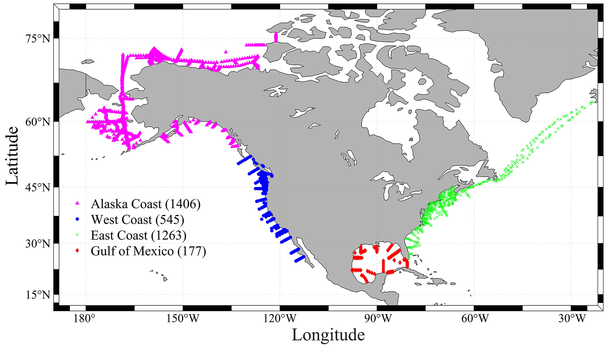
Figure 1 A map showing all the sampling locations of the CODAP-NA data product (v2021, a total of 3391 profiles). Magenta triangles show the sampling profiles at the Alaska coast (AC). Blue ones are for the west coast (WC), green crosses are for the east coast (EC), and the red diamonds are for the Gulf of Mexico (GMx). Numbers within the parentheses indicate the total number of profiles in the region.

2 Study area

From a geopolitical perspective, the term “continental shelf” is defined as the region between the coastline (excluding estuaries) and a distance of 200 nautical miles (∼ 370 km) offshore. While this definition is not as mechanistic as one based on a change in bathymetric gradient or a hydrographic condition such as chlorophyll or salinity levels, it is regionally and seasonally invariant and captures the full extent of coastal influences (Hales et al., 2008). This version of the data product is focused on the continental shelves of the North American coasts (Fig. 1), including

• AC – including the large marine ecosystems (LMEs) of the Gulf of Alaska, eastern Bering Sea, northern Bering–Chukchi seas, and Beaufort Sea (see Sherman et al., 2009, for more information on the LMEs);

• WC – including the LMEs of California Current and Gulf of California;

• EC – including the LMEs of northeast US and southeast US continental shelf regions;

• GMx.

Data beyond continental shelves will be included if they are collected from a cruise that predominately covers parts of the North American ocean margins.

Table 1 Parameters that are included in the CODAP-NA (v2021) data product.

3 Parameters/variables

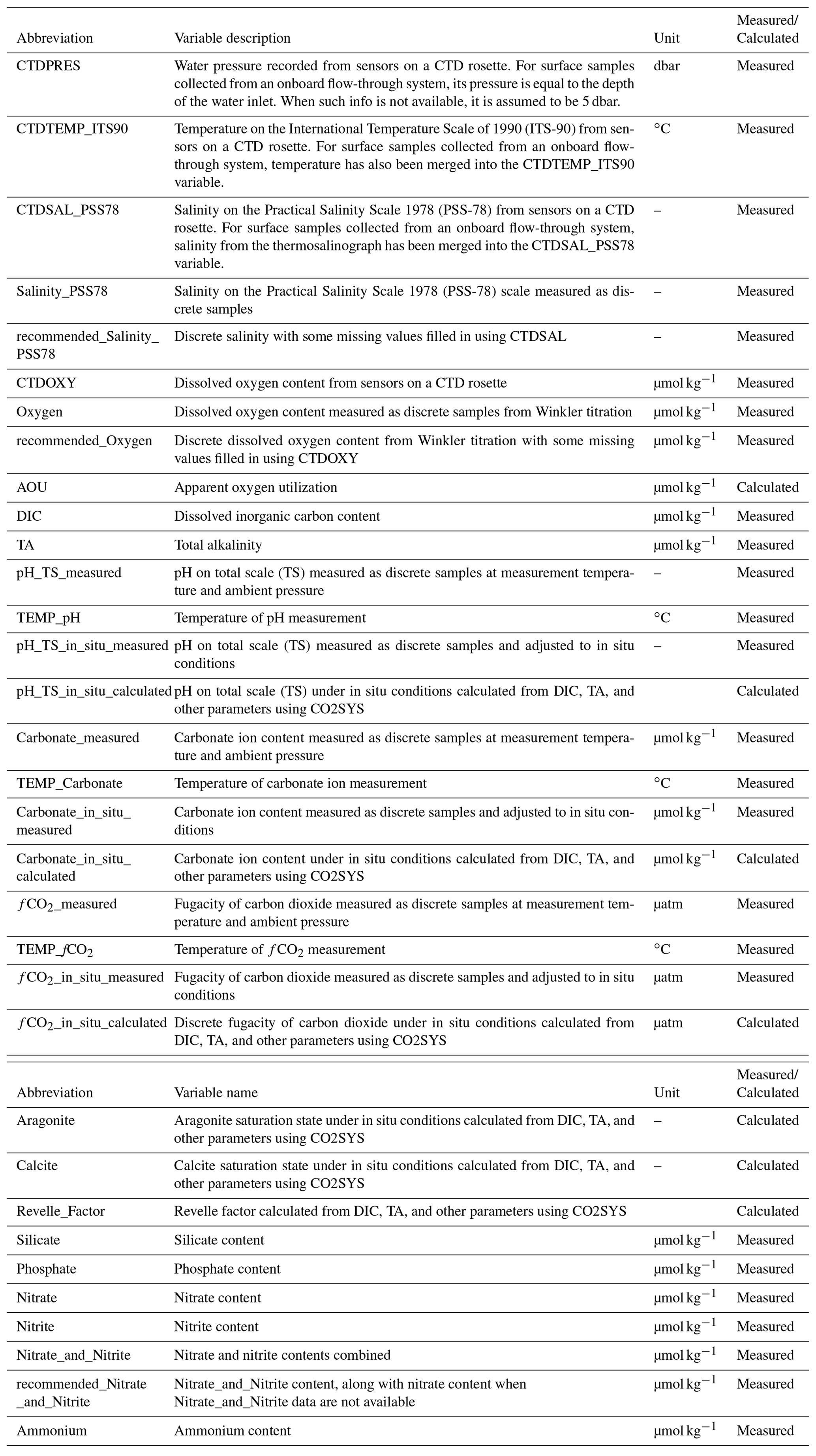
For the current version of the CODAP-NA, inorganic carbon system parameters, oxygen, nutrients, and related hydrographic parameters were included. CTDPRES, CTDTEMP, CTDSAL_PSS78, and CTDOXY were commonly measured with pressure, temperature, conductivity, and oxygen sensors, respectively, mounted on a CTD rosette (Table 1). In some cruises with surface samples collected from flow-through systems, temperature and salinity were also provided in columns reserved for CTDTEMP and CTDSAL_PSS78, respectively. Water samples were routinely collected and measured on board or later in a shore-based laboratory for Salinity_PSS78, Oxygen, DIC, TA, pH_TS_measured, Carbonate_measured, fCO₂_measured, Silicate, Phosphate, Nitrate, Nitrite, Nitrate_and_Nitrite, and Ammonium (Table 1). For pH, carbonate ion content ([CO${}_{\mathrm{3}}^{\mathrm{2}-}$]), and fugacity of carbon dioxide (fCO₂), both measured and calculated values were presented. Saturation states of aragonite (Ω_arag) and calcite (Ω_calc) could only be calculated. The carbon system calculations were conducted using the MATLAB version 3.01 (Sharp et al., 2020) of the CO2SYS program (Lewis and Wallace, 1998), with the dissociation constants for carbonic acid of Lueker et al. (2000), bisulfate (HSO${}_{\mathrm{4}}^{-}$) of Dickson (1990), hydrofluoric acid (HF) of Perez and Fraga (1987), and total borate equations of Lee et al. (2010). Note that the use of “content” (i.e., per kilogram seawater) instead of “concentration” (i.e., per liter) is adopted in this study. For example, either “nitrate content” or “substance content of nitrate” is used instead of “nitrate concentration”. For more information, refer to Jiang et al. (2021b).

Table 2 List of cruises that are included in this version (v2021) of the CODAP-NA data product. Refer to Table 1 for the full names of the abbreviations and their units and Table 3 for definitions of the Cruise_flags. CTD is short for conductivity, temperature, and depth and refers to a package of electronic instruments that measure these properties. Start date and end date refer to the dates when data were first and last collected, respectively. For samples collected from flow-through systems, temperature and salinity were also stored in CTDTEMP and CTDSAL, respectively. GMx is short for Gulf of Mexico. FT is short for flow-through systems.

4 Data sources

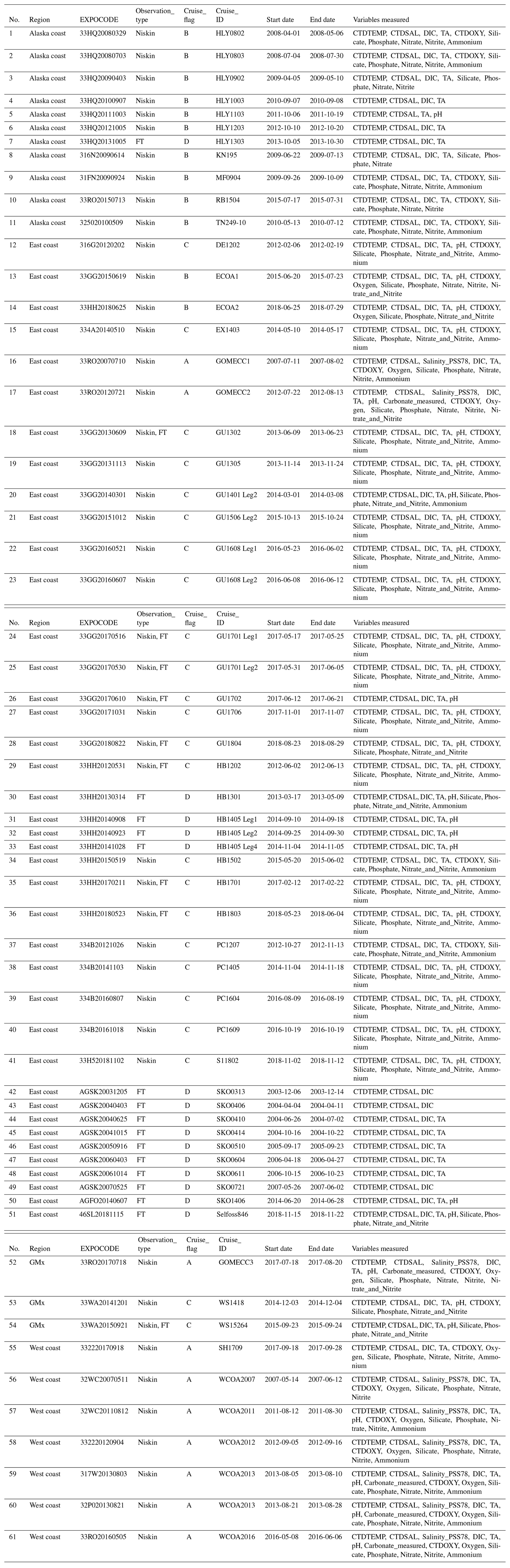
CODAP-NA was focused on chemical oceanographic data (inorganic carbon system parameters, oxygen, and nutrients) collected from discrete sampling-based observations (Table 2). This also included discrete samples taken from shipboard flow-through systems rather than solely water collected in sampling rosette bottles. Carbon parameters recorded from continuous underway measurements by inline analytical instruments were excluded, as they had been quality-controlled and included within the Surface Ocean CO₂ Atlas (SOCAT) (Bakker et al., 2016). The same was true for carbon parameters from time-series moorings. Data from large open estuaries (e.g., Salish Sea, Chesapeake Bay, Bay of Fundy) were excluded during this first round of analysis, but these are among the data that may be able to benefit from second-level QC against CODAP-NA. When a cruise spanned ocean margins and also contained a subset of measurements within estuaries, the estuarine data from that cruise were retained for this data product.

We started with the highest-quality coastal data sets to define a protocol for consistent QC and intercomparison, which would subsequently be applied to other compiled coastal data sets. As a first step, only climate-quality discrete measurements (core data sets) with known quality and metadata from the Atlantic Oceanographic and Meteorological Laboratory, Pacific Marine Environmental Laboratory, University of South Florida, University of Miami, University of Alaska Fairbanks, University of New Hampshire, and University of Delaware were included (Table 2). These data sets will serve as a reference for quality-controlling future data sets.

5 Technical approach and methodology

Cruise data set quality control often involves two steps: primary-level QC and second-level QC (Tanhua et al., 2010). These steps should follow initial, sometimes called “zero-level”, QC, which is performed for individual measurements based on instrument readings and observations collected during the analyses (Fig. 2). Primary-level QC is the process of identifying outliers and obvious errors within an individual cruise data set using measurement metadata or approaches like property-to-property plots. It should largely be done by the investigators responsible for the measurements. In addition, it is critical to provide additional uniform primary-level QC to all cruises within a data product using common tools and common thresholds to help identify any issues that have been missed by the data producers. These issues are communicated back to the investigators so that the issues could be reviewed and, if necessary, addressed. This additional layer of primary-level QC is often performed by the data product synthesis community. Second-level QC is a process in which data from one cruise are objectively compared against data from another cruise or a previously synthesized data set in order to quantify systematic differences in the reported values. The second-level QC process often entails crossover analysis (Lauvset and Tanhua, 2015) and increasingly regional multiple linear regression and inversions (Olsen et al., 2019, 2020).

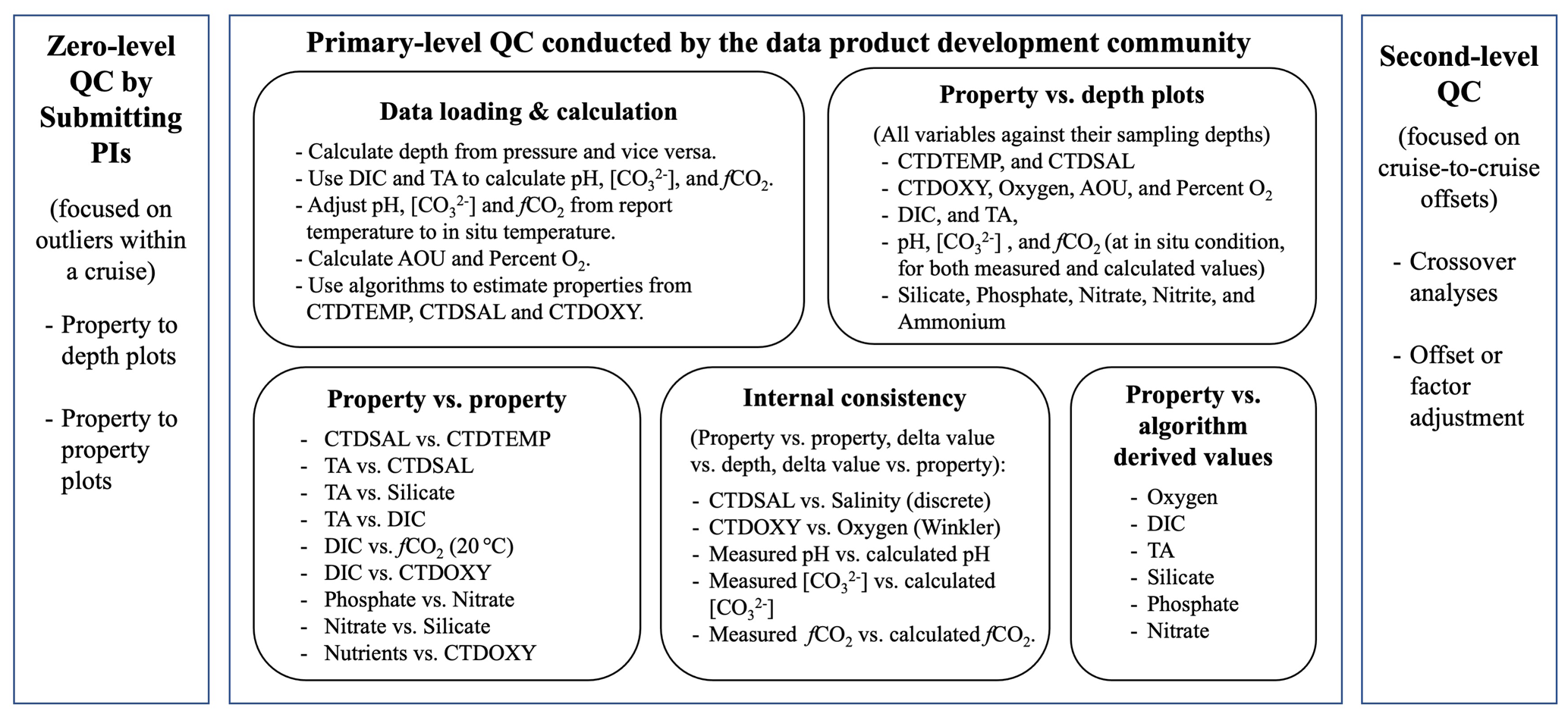
Figure 2 A diagram showing major steps of the quality control (QC) process. Note uncertainty is separated into outliers (scatter) and systematic offset (all data from the cruise has a bias). [CO${}_{\mathrm{3}}^{\mathrm{2}-}$] is carbonate ion content; fCO₂ is fugacity of carbon dioxide. Refer to Table 1 for the rest of the abbreviations.

Due to the scarcity of crossover stations at depths where parameters were not likely to be influenced by temporal variations (sampling depth > 1500 m; Olsen et al., 2020) on coastal cruises, second-level QC was not conducted for this version of the CODAP-NA, and no cruise-wide offsets or multiplicative adjustments were applied. Instead, the QC relied on (a) stringent criteria for the selection of data sources and (b) an enhanced primary-level QC procedure with rigorous consistency checks. This version of the CODAP-NA only accepted data from laboratories with direct involvement in the CODAP effort and with a track record of producing high-quality data and following best practices, making second-level quality control less essential. It is likely that there are other very high quality coastal cruise data sets that are not yet included in this version of CODAP-NA.

We worked directly with the data providers who knew their data best to conduct these primary-level QC procedures in order to leverage all of the resources related to a measurement: details related to the methods, instrumentation, reference standards, access to the raw data, and the analysts' recollection of the measurements. As part of the QC process, comparisons were made between many combinations of measured values. For a subset of properties, inter-consistency calculations and algorithm estimates based on other measurements allowed additional checks. Below are the five major steps of the QC procedures used for CODAP-NA (Fig. 2). A new suite of QC tools is under development to allow these many comparisons and calculations to be performed quickly and efficiently, and these tools will be made available to the public soon with a separate paper dedicated to their rationales, development details, and instructions (Jiang et al., 2021c). A prototype version was used for CODAP-NA, though many software packages would, in principle, allow the comparisons and plots we use.

Step 1 was to ensure all of the cruise data files were ingested into NCEI's archives and documented with a rich metadata record (Jiang et al., 2015b). Maintaining a cruise data table allowing future users of the data product to access the original data files is an important component of any synthesis effort. For this study, a table with key metadata is available through this link: https://www.ncei.noaa.gov/access/ocean-acidification-data-stewardship-oads/synthesis/NAcruises.html (last access: 15 May 2021). The following fields are listed in the table: a sequential number of the individual cruise data set (no.), expedition code (EXPOCODE), flags indicating the quality of the cruise (Cruise_flag; see Table 3), cruise identifier (Cruise_ID), start date, end date, measured parameters, and links to NCEI's archive.

Table 3 Cruise flags used for this product.

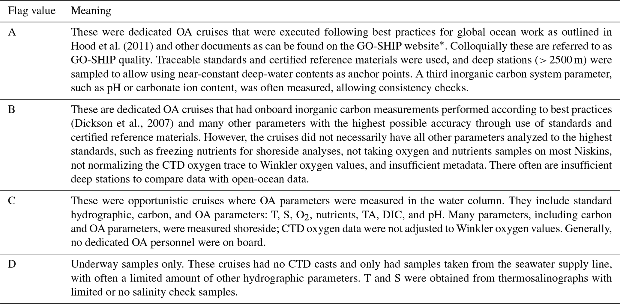
^* https://www.go-ship.org/HydroMan.html (last access: 15 May 2021)

Table 4 World Ocean Circulation Experiment (WOCE) World Hydrographic Program (WHP) (Joyce and Corry, 1994; Swift and Diggs, 2008) QC flags used for this product.

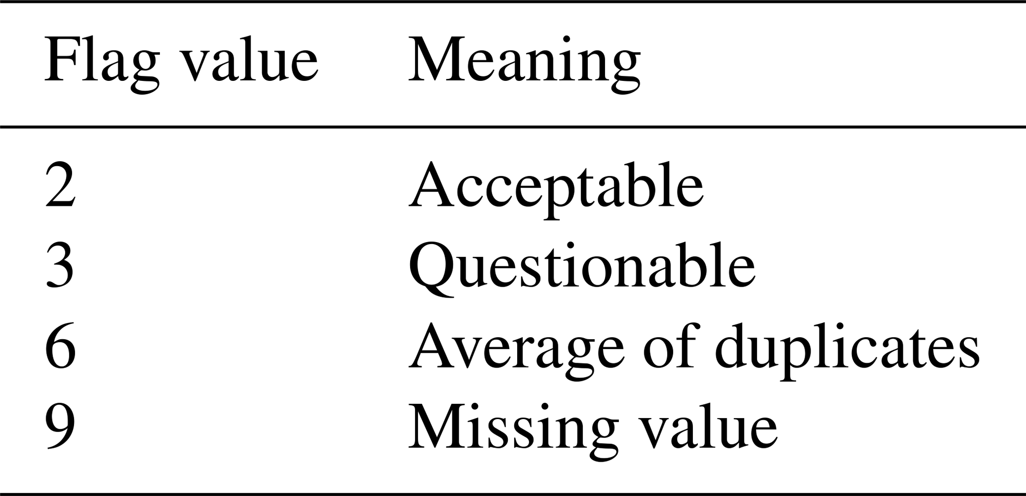
Step 2 was to load the measurement values from the original cruise data files into MATLAB and conduct necessary calculations (Fig. 2). All missing values were replaced with “-999” during this process. Variables without a QC flag from the original cruise data file were assigned an initial flag of “2” (good values, Table 4). Variables that were clearly out of range (e.g., a DIC value of < 0) were automatically assigned a QC flag of “4” (bad values). The QC flags for all -999 values or missing values were replaced with “9” (missing values). All bottle measurement flags with a corresponding Niskin_flag of 3 or 4 were replaced with the corresponding Niskin_flags. For example, if a discrete salinity measurement has a Salinity_flag of 2 but the corresponding Niskin_flag (QC flag of the Niskin bottle where the sample was drawn) is 3, the original Salinity_flag will be updated from 2 to 3.

Some surface samples from a few coastal cruises were collected from flow-through systems on board research vessels, instead of Niskin bottles on sampling rosettes. In such cases, the temperature and salinity values were stored under the CTDTEMP and CTDSAL columns, respectively, although they were not measured from sensors mounted on a CTD rosette. Similarly, their sampling depth values were extracted from the metadata as the depth of the water inlet and stored under CTDPRES (Table 1). When water inlet depth information was not available, its sampling pressure was set to be 5 dbar. There is a column named “Observation_type” in the CODAP-NA data product file to indicate whether a sample is from a “Flow-through” system or a “Niskin” bottle.

We calculated or assigned the below parameters:

• a.

  Sample_ID if not already included (Eq. 1);

• b.

  depth from pressure and vice versa;

• c.

  recommended_Salinity_PSS78 (Table 1);

• d.

  conservative temperature, absolute salinity, and sigma-theta;

• e.

  recommended_Oxygen;

• f.

  apparent oxygen utilization (AOU);

• g.

  recommended_Nitrate_and_Nitrite;

• h.

  calculated pH, carbonate ion, and fCO₂ under in situ conditions using CO2SYS from DIC and TA, along with temperature, salinity, pressure, and nutrients;

• i.

  in situ pH, carbonate ion, and fCO₂ from their respective values under their measurement conditions.

Sample_IDs were calculated from Station_ID (station identification number), Cast_number (cast number), and Niskin_ID (Niskin identification) based on Eq. (1) if they were not already available:

$$\begin{array}{}\text{(1)}& \begin{array}{rl}\text{Sample\_ID}& =\text{Station\_ID}\times \mathrm{10}\mathrm{000}+\text{Cast\_number}\times \mathrm{100}\\ & +\text{Niskin\_ID}.\end{array}\end{array}$$

For example, at station 15, the second cast, a Niskin_ID of 3 will have a Sample_ID of 150203. In cases when they could not be calculated (e.g., Station_ID is non-numerical), Sample_ID was assigned as 1, 2, 3, … from the first row to the last row of the original cruise data file.

Sampling depth (Depth) and pressure (CTDPRES) were calculated from one another where applicable using the equations of “gsw_z_from_p” and “gsw_p_from_z”, respectively, from the International Thermodynamic Equation of Seawater 2010 (TEOS-10; IOC et al., 2010). When both values were available, CTDPRES values were preferentially used, and the calculated Depth values were used to replace the original Depth values.

The “recommended_Salinity_PSS78” column was created by merging the discrete salinity and CTDSAL columns. Data were preferentially chosen from the discrete measurements provided their QC flags were equal to 2 or 6. If these values were not available, CTDSAL values with QC flags of 2 or 6 were chosen. In the absence of these two, discrete salinity measures with QC flags other than 2 or 6 were chosen. Lastly, the CTDSAL values with other QC flags were chosen. The same principles were applied to merge the oxygen data. The merged discrete oxygen and CTDOXY data were stored in the column named “recommended_Oxygen” (Table 1).

Conservative temperature (Θ) is proportional to the potential enthalpy and is recommended as a replacement for potential temperature (θ), as it more accurately represents the heat content (IOC et al., 2010). Absolute salinity (S_A) is the mass fraction of salt in seawater (unit: g kg⁻¹) based on conductivity ratio plus a regional correction term as opposed to the practical salinity scale (S_P, Practical Salinity Scale 1978, or PSS-78; unitless; based solely on the conductivity ratio) (Le Menn et al., 2018). Conservative temperature, absolute salinity, and sigma-theta were calculated using the equations of “gsw_CT_ from_t”, “gsw_SA_from_SP”, and “gsw_sigma0”, respectively, from the TEOS-10 (IOC et al., 2010). AOU was calculated based on absolute salinity, conservative temperature, latitude, longitude, CTDPRES, and recommended_Oxygen variable using the function “gsw_O2sol” as described in the TEOS-10 (IOC et al., 2010). Oxygen solubility is estimated with the combined equation from Garcia and Gordon (1992).

In order to measure nitrate, it is first reduced to nitrite, and then this new nitrite is measured alongside the nitrite originally in seawater (Hydes and Hill, 1985). The substance content of nitrite in ocean water is usually much lower than nitrate. When nitrite is not reported, it is often because its content is too low to be detectable. For the CODAP-NA data product, when Nitrate values were not available but both Nitrate_and_Nitrite and Nitrite values with QC flags of 2 or 6 were available, Nitrate values were calculated by subtracting Nitrite from Nitrate_and_Nitrite. Similarly, when Nitrate_and_Nitrite values were not available but both Nitrate and Nitrite values with QC flags of 2 or 6 were available, Nitrate_and_Nitrite values were calculated by adding Nitrate and Nitrite contents together. The “recommended_Nitrate_and_Nitrite” column was created by preferentially using Nitrate_and_Nitrite values. In cases when Nitrate_and_Nitrite values were not available but Nitrate values with a QC flag of 2 or 6 were available (Nitrite values not available), the Nitrate_and_Nitrite values were assumed to equal the Nitrate values.

Carbonate_in_situ_measured, pH_TS_in_situ_measured, and fCO₂_in_situ_measured (Table 1) were recalculated from their respective values under measurement conditions (i.e., pH_TS_measured, Carbonate_measured, and fCO₂_ in_situ_measured) with the CO2SYS program, using the dissociation constants as described above. TA was preferentially used as the second carbon parameter. When it was not available, DIC was used. If neither of them was available, TA derived from salinity with the locally interpolated alkalinity regression (LIARv2) method was used for the adjustment from measurement to in situ conditions (Carter et al., 2018). Carbonate_in_situ_calculated, pH_TS_in_situ_calculated, fCO₂_in_situ_calculated, aragonite saturation state, calcite saturation state, and Revelle_Factor were calculated from DIC and TA, along with in situ temperature, salinity, pressure, silicate, and phosphate using the same dissociation constants as above (Table 1). When either silicate or phosphate data were unavailable, their mean values during the cruise were used for the calculation. Samples with a salinity of less than 15 were excluded from this calculation, due to the potentially large uncertainties.

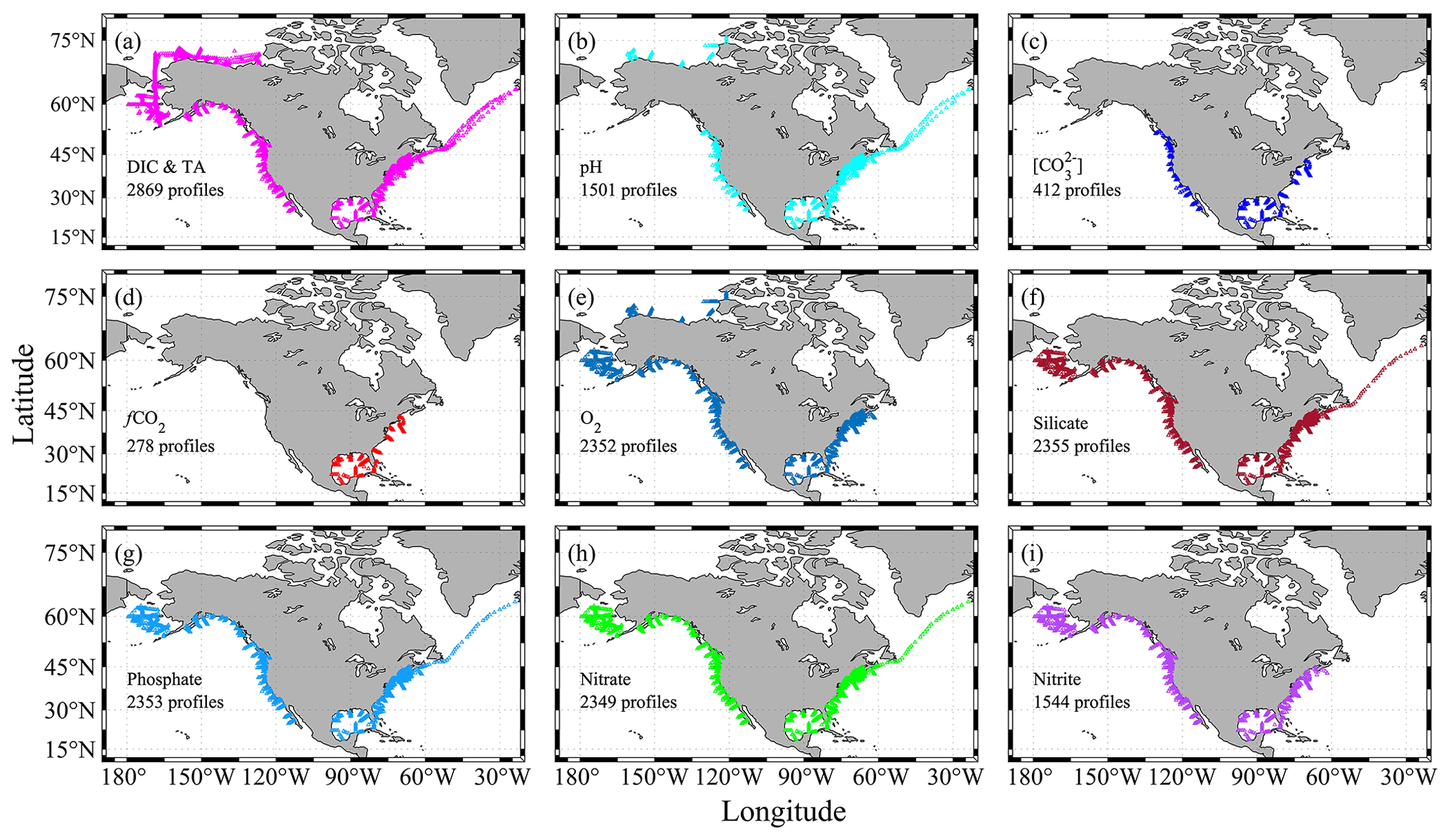
Figure 3 Sampling profiles for certain parameters. A profile is plotted if it has at least one measured value. Panel (a) only includes profiles that have both dissolved inorganic carbon (DIC) and total alkalinity (TA) measured. Panel (b) is for profiles with discrete pH measurements from a spectrophotometer. Panel (c) is for profiles with discrete carbonate ion content ([CO${}_{\mathrm{3}}^{\mathrm{2}-}$]) measurements from a spectrophotometer. Panel (d) is for profiles with discrete fugacity of carbon dioxide (fCO₂) measurements from flasks. Panel (e) is for profiles with recommended_Oxygen values (see Table 1 for more details). Panels (f)–(i) are for profiles with nutrient measurements.

Step 3 was to identify outliers. Outliers were determined by visual inspection. Two types of outlier identification were used for this effort: (a) a broad-scale outlier identification by visually examining the plot of a variable against its sampling depth and other property-to-property plots and (b) a fine-scale outlier identification based on consistency checks. Here, consistency checks refer to both the “internal consistency checks” – i.e., the comparison of a measurement with its calculated value (e.g., spectrophotometrically measured pH vs. pH calculated from other carbon parameters using CO2SYS) – and validation checks, i.e., a measurement with one method against the same measurement made with a different method (e.g., oxygen measured from Winkler titration vs. a sensor, though in this case the oxygen profile is frequently adjusted to the Winkler titration values, so the measurements are not truly independent). For the broad-scale outlier identification we made plots of all variables against depth (or sigma-theta when only surface values are available), as well as these plots (Fig. 2):

• a.

  CTDSAL against CTDTEMP

• b.

  TA against CTDSAL

• c.

  TA against Silicate

• d.

  TA against DIC

• e.

  DIC against fCO₂ (20 ^∘C)

• f.

  DIC against CTDOXY

• g.

  Phosphate against Nitrate

• h.

  Nitrate against Silicate

• i.

  all nutrients (silicate, phosphate, nitrate, nitrite, nitrate plus nitrite, and ammonium) against CTDOXY.

Consistency-check-based outlier identification was the primary way of finding outliers in this study. Consistency checks were conducted for these below variable pairs. This has been the most effective way of identifying outliers.

• a.

  CTDSAL vs. discrete salinity (discrete salinity as the reference value);

• b.

  CTDOXY vs. discrete oxygen measured from Winkler titration (Winkler oxygen as the reference value);

• c.

  pH measured with a spectrophotometer vs. pH calculated with CO2SYS from DIC, TA, and other parameters;

• d.

  Carbonate ion ([CO${}_{\mathrm{3}}^{\mathrm{2}-}$]) measured with a spectrophotometer vs. [CO${}_{\mathrm{3}}^{\mathrm{2}-}$] calculated with CO2SYS from DIC, TA, and other parameters;

• e.

  Discrete fCO₂ measured with a non-dispersive infrared analyzer vs. fCO₂ calculated with CO2SYS from DIC, TA, and other parameters.

In addition, the values for dissolved oxygen, DIC, TA, Silicate, Phosphate, and Nitrate were also calculated from existing estimation algorithms (e.g., Carter et al., 2018). These estimates were then compared against the measured CTDOXY and Oxygen, DIC, TA, Silicate, Phosphate, and Nitrate, respectively, to help assess whether cruise-to-cruise biases exist (Fig. 2). These algorithms are intended primarily for open-ocean estimation. They are used in the coastal environment only to call attention to measurements that require additional QC, and never to directly assign flags.

For all the aforementioned plots, we enable features to go through each profile individually with all data from a cruise plotted together in the background. Similarly, we are able to go through each cruise individually with all data from all cruises plotted together in the background. These approaches allow us to detect systematic offsets.

Step 4 was to append all of the individual cruise data files one after another into one data product file with all of the variables as listed in Table 1. All rows with a Niskin_flag of 4 (Table 4) were removed. Data values with QC flags that were not 2 (good), 3 (questionable), or 6 (average of duplicate measurements) were replaced with -999, and their corresponding QC flags were changed to 9. For surface samples collected from flow-through systems, their Cast_numbers and Niskin_IDs were all set to -999, and their Niskin_flags were all set to 9. The contents of Observation_type were standardized to be either Niskin or Flow-through. The merged data product file was further quality-controlled by plotting all of the non-missing values for each variable. These plots were examined further, with focus on the outliers falling out of 2.5 times their respective standard deviations.

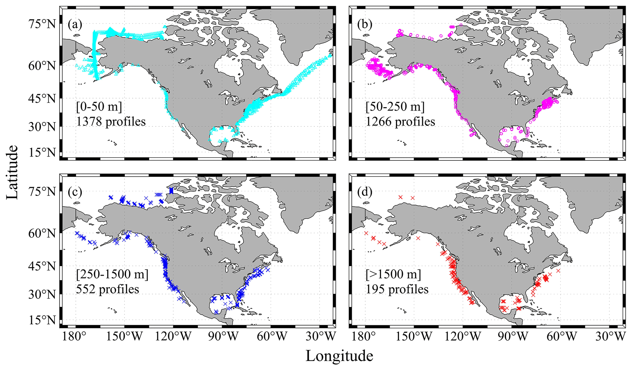
Figure 4 Sampling depths of the profiles: (a) profiles with maximum depths ranging from 0 to 50 m, (b) profiles with maximum depths ranging from 50 to 250 m, (c) profiles with maximum depths ranging from 250 to 1500 m, and (d) profiles with maximum depths greater than 1500 m.

Table 5 The minimum, maximum, mean, and data point counts of the parameters that are included in the final product. Refer to Table 2 for their full parameter names and units.

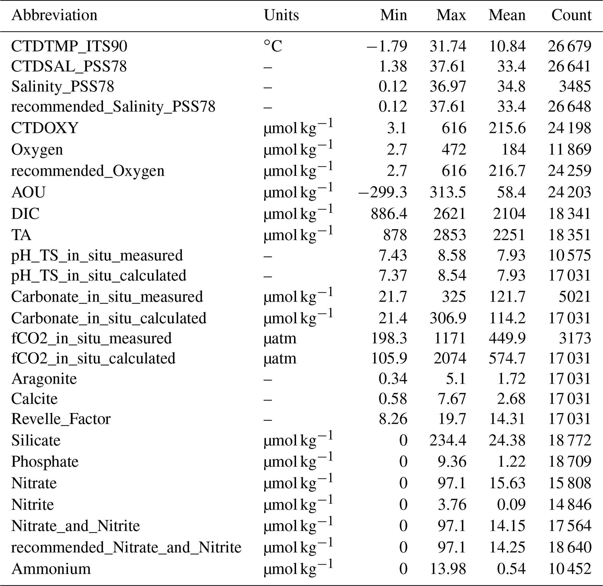
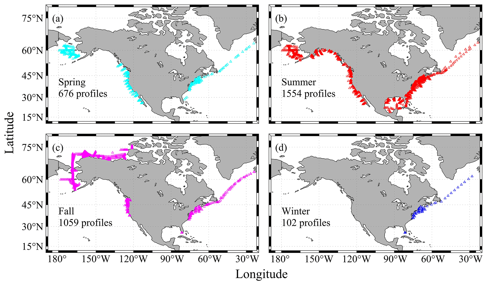
Figure 5 Sampling profiles in each of the four seasons: (a) spring (March–May), (b) summer (June–August), (c) fall (September–November), and (d) winter (December–February).

6 Data products

The data product is available in Excel, CSV, MATLAB, and NetCDF formats at NOAA/NCEI with a DOI of https://doi.org/10.25921/531n-c230 and NCEI accession number of 0219960 (Jiang et al., 2021a). All parameters in Table 1 along with their Cruise_flags (Table 3) and primary-level QC flags (Table 4) are presented. The chosen primary-level QC flag convention is the same as the GLODAPv2 project (Olsen et al., 2020). Note the difference between the WOCE primary-level QC flags (e.g., 2, 3, 4, 9, etc.) and the second-level QC flags as used by the GLODAPv2 (a choice of either 0 or 1). In the current version (v2021) of the CODAP-NA, there are 3391 discrete chemical oceanographic profiles and a total of 28 206 data points. They were collected on 61 cruises in the ocean margins of North America from 6 December 2003 to 22 November 2018. There are on average eight sampling depth levels (a median of seven) for each profile. The total count of data points for each parameter and their minimum, maximum, and mean values are listed in Table 5.

Of the 3391 profiles, 2869 have both DIC and TA measurements; thus the full list of carbonate system parameters (pH, fCO₂, [CO${}_{\mathrm{3}}^{\mathrm{2}-}$], aragonite saturation state, calcite saturation state, and Revelle factor) can be calculated (Fig. 3). In addition, there are 1501 profiles with discrete pH measurements from a spectrophotometer-based method (Byrne and Breland, 1989; Clayton and Byrne, 1993; Dickson, 1993), 412 profiles with discrete carbonate ion measurements (Byrne and Yao, 2008; Sharp and Byrne, 2019), and 278 profiles with discrete fCO₂ measurements (Wanninkhof and Thoning, 1993). There is also good coverage of oxygen and nutrients measurements (Fig. 3).

One major difference between the CODAP-NA and the GLODAPv2 is the shallower sampling depths of the former (Fig. 4). About 80 % of the 3391 profiles have a maximum sampling depth of < 250 m, and 30 % of them have maximum sampling depth of < 25 m, with a lot of them being surface-only measurements. Only 195 profiles (< 6 % of the total 3391 profiles) have at least one sampling depth level below 1500 m, which has commonly been used as a threshold for subsurface crossover analyses (Fig. 4). Most of these deep-water profiles are found off the west coast, Gulf of Mexico, and a few offshore stations in the Mid-Atlantic Bight. On average, the sampling depth is 298 m, with a median sampling depth of only 65 m.

Another distinctive feature of coastal oceans is their large magnitude of seasonal variation. For a lot of parameters, their seasonal variation, along with the diel and intertidal variations, often eclipse their long-term variation. Understanding the seasonal variation and de-seasonalizing the observation data are often critical steps in the process of deciphering the long-term change. Like most data products, this version of the CODAP-NA is summer- and fall-biased, with spring, summer, fall, and winter having 676, 1554, 1059, and 102 profiles, respectively (Fig. 5). All coasts have good summer data coverage, but the only area with meaningful winter data coverage is the northeastern US coast (Fig. 5, Table 6).

Table 6 Number of profiles and data points (the sum of all depth levels at each profile) in all seasons of each region.

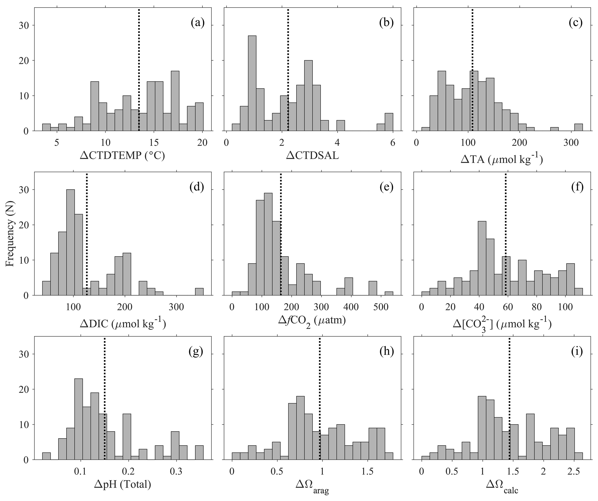
Figure 6 Seasonal amplitudes (maximum minus minimum values within a group of close by stations) of (a) temperature (CTDTEMP), (b) salinity (CTDSAL), (c) total alkalinity (TA), (d) dissolved inorganic carbon (DIC), (e) fugacity of carbon dioxide (fCO₂), (f) carbonate ([CO${}_{\mathrm{3}}^{\mathrm{2}-}$], (g) pH on total scale, (h) aragonite saturation state (Ω_arag), and (i) calcite saturation state (Ω_calc) in the surface water. The y axis, “frequency (N)”, refers to the number of groups of stations. The dotted lines show the average value of the variabilities. This analysis is based on groups of profiles that are within 1 km of each other.

To demonstrate the large seasonal amplitude (defined here as the difference between the maximum and minimum values of a variable on an annual cycle) in the study area, an analysis was conducted to group surface stations (with at least one sampling depth < 25 m) that are within 1 km distance and have at least one measurement between December and March and one measurement between June and October. The results, which are based on 135 groups of stations (most of them along the northeastern US coast), show large seasonal variations for nearly all the variables (Fig. 6). The average seasonal amplitudes and their percentage changes are CTDTEMP (13.9 ^∘C), CTDSAL (2.3), TA (112 µmol kg⁻¹, 5 %), DIC (126 µmol kg⁻¹, 6 %), fCO₂ (170 µatm, 39 %), [CO${}_{\mathrm{3}}^{\mathrm{2}-}$] (61 µmol kg⁻¹, 45 %), pH (0.16), aragonite saturation state (0.99, 47 %), and calcite saturation state (1.47, 45 %). Note the “seasonal amplitudes” here represent the sum of effects of all changes including changes from freshwater input, mixing, upwelling, warming and cooling, biological cycling, and diurnal cycling within a season.

Table 7 Uncertainties of some variables based on an analysis that groups deep-water stations (> 1000 m sampling depth) within a 10 km radius and 200 m depth difference. SD is short for standard deviation. Numbers in parentheses are expected errors based on propagating uncertainties in carbonate system calculations using DIC, TA, and others as input parameters with the CO2SYS companion errors.m program. Refer to Table 1 for their full names and respective units.

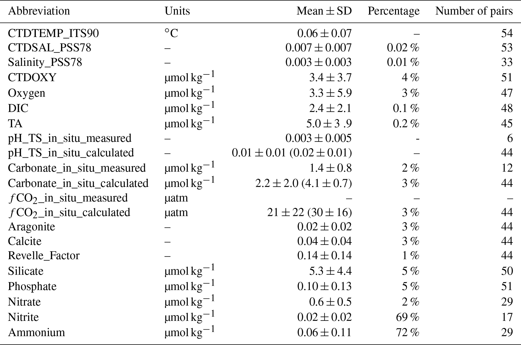
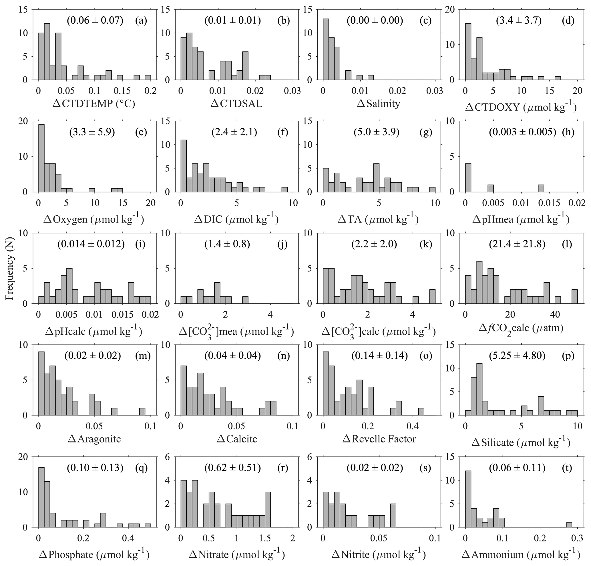
Figure 7 Uncertainties of some parameters based on deep-water comparison analyses: (a) temperature (ITS-90) measured with CTD sensors; (b) salinity (PSS78) measured with CTD sensors; (c) discrete salinity (PSS78); (d) dissolved oxygen measured with CTD sensors; (e) dissolved oxygen content measured with Winkler titration; (f) dissolved inorganic carbon content; (g) total alkalinity; (h) pH on total scale measured with spectrophotometers; (i) pH on total scale calculated from DIC, TA, and other parameters; (j) carbonate ion content measured with spectrophotometers; (k)–(o) carbonate ion content, fugacity of carbon dioxide, aragonite saturation state, calcite saturation state, and Revelle factor calculated from DIC, TA, and other parameters; and (p)–(t) Silicate, Phosphate, Nitrate, Nitrite, and Ammonium contents. The y axis, “frequency (N)”, refers to the number of groups of stations. The values inside the parentheses are mean values ± standard deviations.

To present a rough estimate of the measurement uncertainties of these variables, a similar approach was used to group deep-water stations with a maximum sampling depth of > 1500 m. Due to the scarcity of deep-water stations, a radius of 10 km and 200 m depth difference were used to find the comparison pairs. This analysis is limited to certain cruises with deep-water sampling (∼ 5 % of the data) only; thus the uncertainty estimates only hold true for these “reference” cruises, mostly with a Cruise_flag of A (Table 3). They do not apply to the rest of the cruises. Results show that the DIC and TA uncertainties (0.1 % and 0.2 %, respectively) are about the same as previously reported by the GLODAPv2 group (Fig. 7, Table 7) by this metric. Some variables like Nitrite and Ammonium show uncertainties as large as ∼ 70 % with this metric due, primarily, to the low average values of these measurements at depth. The average CTDTEMP precision of 0.06 ^∘C is significantly higher than that of 0.01 ^∘C as previously reported for the GLODAPv2 (Olsen et al., 2020). The measurement uncertainties could be overestimated, because this analysis includes natural gradients due to the large radius and depth differences, as well as any temporal changes within the 1–10-year (average: 6-year) period.

For aragonite and calcite saturation states, uncertainty comes primarily from the use of an empirical equation to approximate the real-world apparent solubility product (${K^{\prime }}_{\text{sp}}$). Despite the 3 % number shown in Table 7, the real uncertainty of aragonite and calcite saturation states is likely > 5 % (Mucci, 1983; Jiang et al., 2015a; Orr et al., 2018). Best practices for oceanic carbonate system calculations have been recommending the dissociation constants of Lueker et al. (2000) (Dickson et al., 2007). However, a recent study finds that in colder regions, where water temperature is < 8 ^∘C, the constants of Lueker et al. (2000) may underestimate fCO₂ and overestimate pH and [CO${}_{\mathrm{3}}^{\mathrm{2}-}$], meaning that cold ocean regions could be more undersaturated than expected with respect to calcium carbonate mineral (CaCO₃) saturation states (Sulpis et al., 2020). This applies to many Alaska coast stations. In brackish water (salinity < 20), the relative uncertainty in carbonate ion content is worse than that in open ocean water (Dickson et al., 2007; Orr et al., 2018). In addition, due to the way calcium content is derived in the CO2SYS (Riley and Tongudai, 1967; Millero, 1995), the calculated saturation states could suffer from uncertainties up to 12 % for not directly measuring the calcium content in certain very low salinity regions (Beckwith et al., 2019; Dillon et al., 2020).

Note the above uncertainty analyses are based on deep-water stations only, and these data are usually collected from cruises with a Cruise_flag of A or B (Table 3). The uncertainties of data points from cruises with Cruise_flags of C and D are expected to be much larger. Internal consistency checks of measured versus calculated values and validation checks of values measured using different methods show that differences increase quickly towards the surface (Figs. 8–11). Some apparent “outliers” end up being in surface samples where the Niskin vs. CTD values are offset due to highly stratified surface conditions in the coastal ocean. We contend that these Winkler and CTD values are likely “good” data from the measurement point of view, so, for such instances, the QC flags are kept as 2, despite their poor internal consistency.

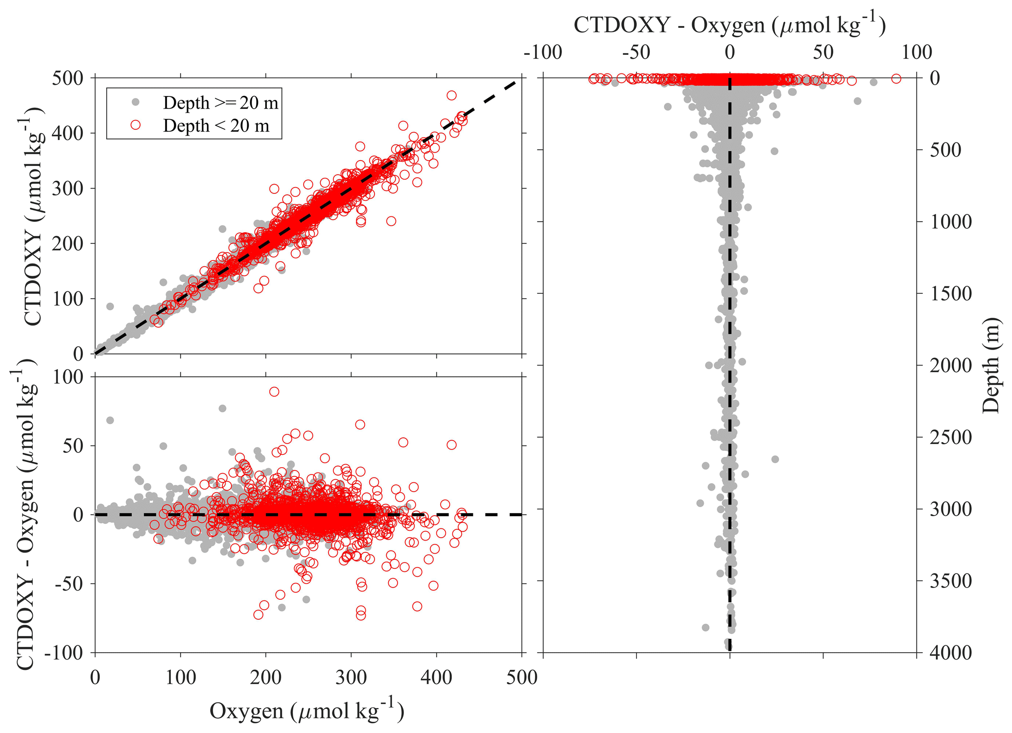
Figure 8 Comparison plots of dissolved oxygen measured from sensors mounted on CTD (CTDOXY) and dissolved oxygen that is measured from Winkler titration (Oxygen).

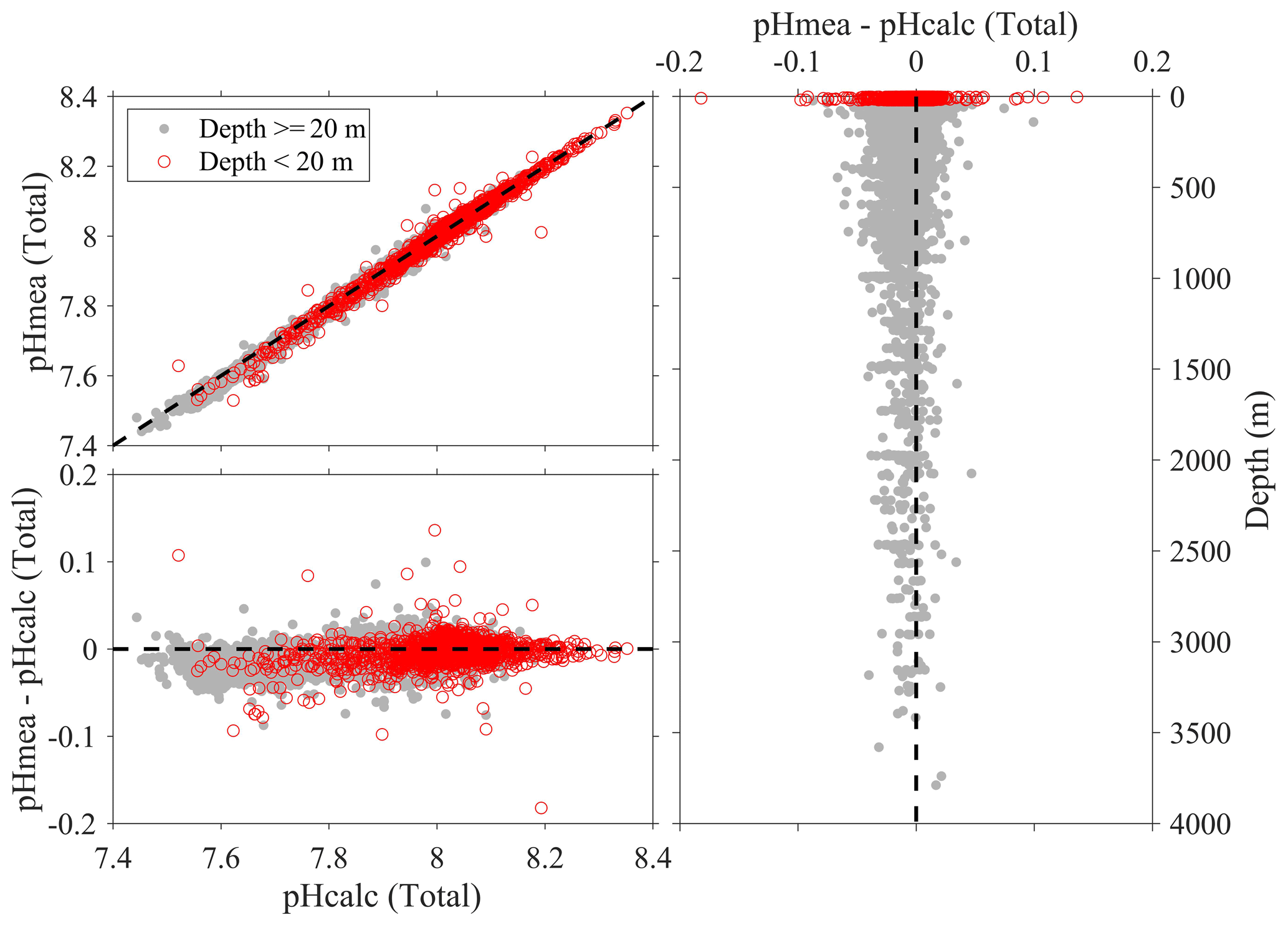
Figure 9 Comparison plots of in situ pH (total scale) that is measured using spectrophotometers (pHmea) and in situ pH (total scale) that is calculated from DIC and TA and other parameters (pHcalc).

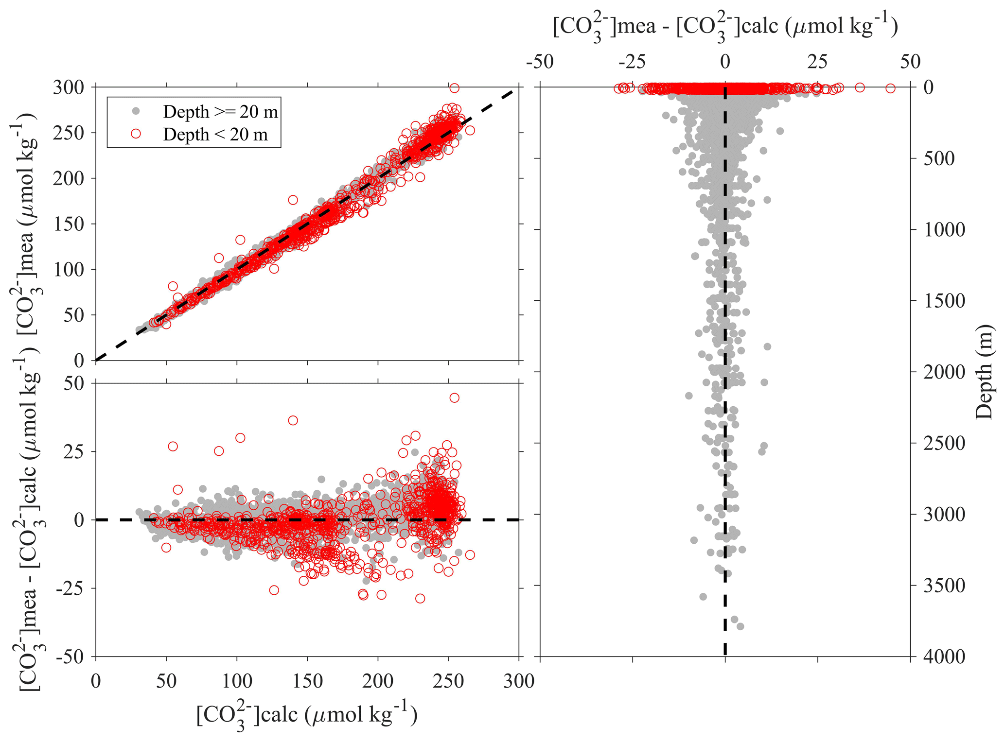
Figure 10 Comparison plots of in situ carbonate ion content that is measured using spectrophotometers ([CO${}_{\mathrm{3}}^{\mathrm{2}-}$]mea) and that is calculated from DIC, TA, and other parameters ([CO${}_{\mathrm{3}}^{\mathrm{2}-}$]calc).

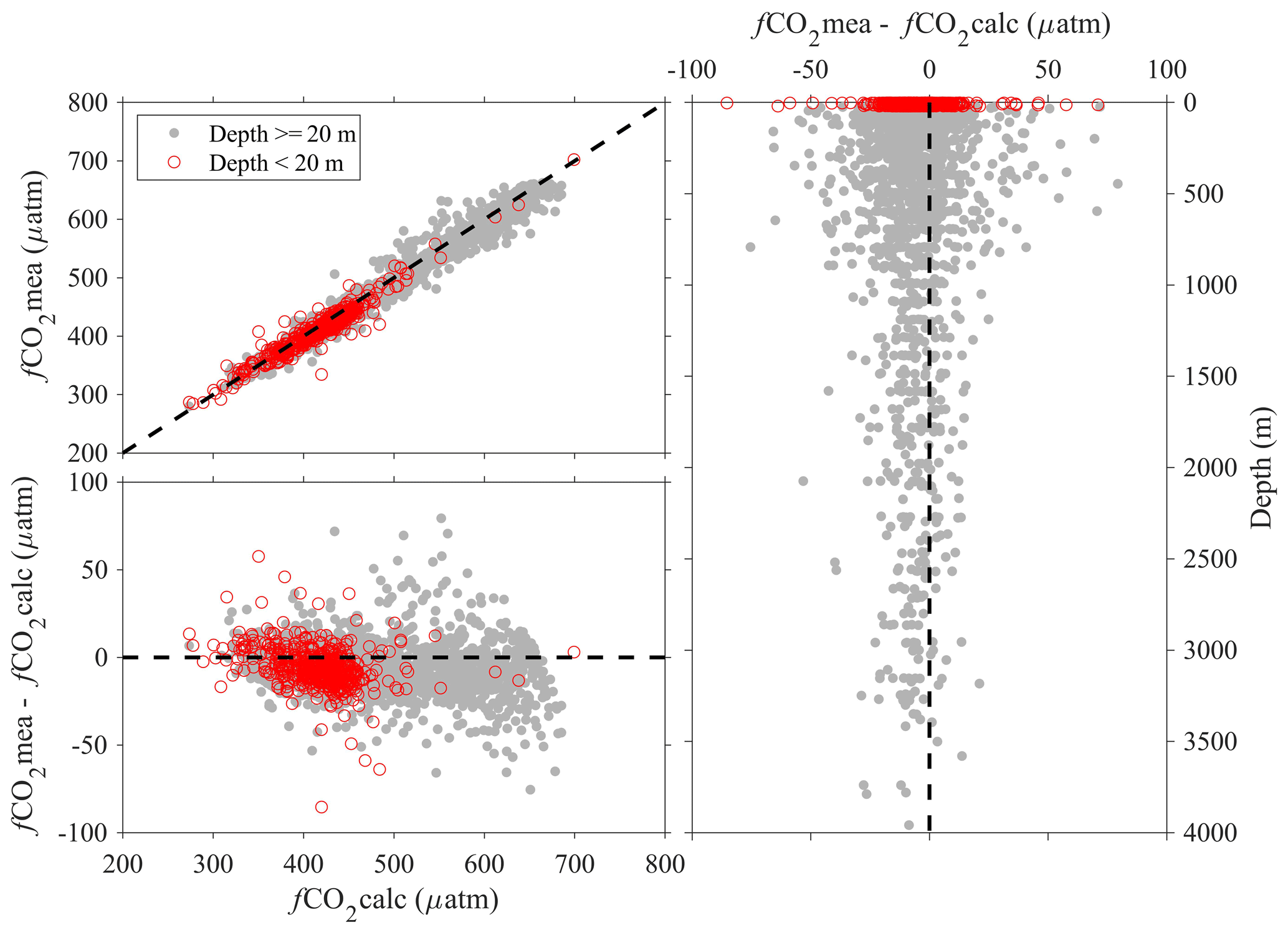
Figure 11 Comparison plots of fugacity of carbon dioxide (fCO₂mea) that is measured from discrete bottle samples and fCO₂ that is calculated from DIC, TA, and other parameters (fCO₂calc).

7 Data availability

The Coastal Ocean Data Analysis Product in North America (CODAP-NA) is available as a merged data product in the formats of Excel, CSV, MATLAB, and NetCDF (https://doi.org/10.25921/531n-c230; NCEI Accession: 0219960) and can be accessed with the following link: https://www.ncei.noaa.gov/data/oceans/ncei/ocads/metadata/0219960.html (last access: 15 May 2021) (Jiang et al., 2021a). An Excel spreadsheet listing all of the QC-related changes is also included as part of the data package. The original cruise data files have also been updated with data providers' consent and summarized in a table with the following link: https://www.ncei.noaa.gov/access/ocean-acidification-data-stewardship-oads/synthesis/NAcruises.html (last access: 15 May 2021).

8 Summary and conclusions

In this study, we relied on consistency checks performed in direct collaboration with the data providers who originally collected and measured the samples to QC and synthesize 2 decades of discrete measurements of inorganic carbon system parameters, oxygen, and nutrient chemistry data from North America's coastal oceans. The generated data product is called Coastal Ocean Data Analysis Product in North America (CODAP-NA). It is composed of 3391 oceanographic profiles from 61 research cruises covering all continental shelves in North America (west coast, east coast, Gulf of Mexico, and Alaska coast) from 6 December 2003 to 22 November 2018.

It is strongly recommended to measure a third carbon-related variable for consistency check purposes. The large majority of coastal OA cruises have already measured DIC and TA, with a lot of them also measuring pH using high-precision spectrophotometric methods. Recently, laboratories have increasingly begun to include carbonate ion content ([CO${}_{\mathrm{3}}^{\mathrm{2}-}$]) as an additional measurable parameter of the seawater CO₂ system (Byrne and Yao, 2008; Sharp and Byrne, 2019). Uncertainty analyses suggest that crossover adjustments could be applied to future coastal data QC. All major coastal cruises in the future are recommended to take deep-water samples (> 1500 m) when feasible, ideally at agreed-upon reference stations for QC purposes.

Quality control of coastal data is an ongoing challenge that is not fully resolved by this effort, but CODAP-NA provides a foothold for future efforts toward continuously updating CODAP-NA as an internally consistent data product for the coastal environment. Perhaps more significantly, the CODAP-NA product greatly improves the findability, accessibility, interoperability, and reusability of these data sets. Findability is improved with this paper highlighting the data sets, accessibility is improved through data ingestion of the cruises in Table 2 into a coherent data product, interoperability is improved by providing the product in multiple machine-readable formats, and reusability is improved by assigning a static DOI for this initial version of the product.