tTEM20AAR: a benchmark geophysical data set for unconsolidated fluvioglacial sediments

Quaternary deposits are complex and heterogeneous. They contain some of the most abundant and extensively used aquifers. In order to improve the knowledge of the spatial heterogeneity of such deposits, we acquired a large (1500 ha) and dense (20 m spacing) time domain electromagnetic (TDEM) data set in the upper Aare Valley, Switzerland (available at https://doi.org/10.5281/zenodo.4269887; Neven et al., 2020). TDEM is a fast and reliable method to measure the magnetic field directly related to the resistivity of the underground. In this paper, we present the inverted resistivity models derived from this acquisition. The depth of investigation ranges between 40 and 120 m, with an average data residual contained in the standard deviation of the data. These data can be used for many different purposes: from sedimentological interpretation of quaternary environments in alpine environments, geological and hydrogeological modeling, to benchmarking geophysical inversion techniques.

1 Background and summary

In most urbanized and agricultural areas of Switzerland, the shallow underground is constituted of Quaternary deposits. The thickness can vary from few meters to hundreds of meters. These recent sediments are deposited by various agents such as rivers, lakes, glaciers, or even landslides. Each time, the associated sediment will have a different composition and permeability and a spatial variability that is often higher than expected in such deposits.

However, these formations are some of the most solicited: water supply for cities, extraction of construction materials, and shallow geothermal exploitation. Often, the construction of geological models using only boreholes can miss most of the spatial heterogeneity and lead to inadequate models and wrong conclusions. Increasing the number of boreholes to reduce the uncertainty is often difficult and expensive. A good example of these highly exploited Quaternary zones is the upper Aare Valley (Fig. 1). In 60 km², the Aare Valley includes 4 quarries, 6350 pumping wells (shallow geothermic or drinkable water), and 5300 injection wells (re-inject water after geothermal heat pump). A previous valley size model was designed using boreholes and surface data (Volken et al., 2016), but the model does not represent the internal heterogeneities of the Quaternary formations and can show unrealistic sharp variations due to the nearest-neighbor interpolation method used during the workflow. Therefore, there is a need for a better understanding of Quaternary sedimentary heterogeneity, in order to better constrain geological models, knowledge that could be applied in the Aare Valley or for any fluvioglacial filling area.

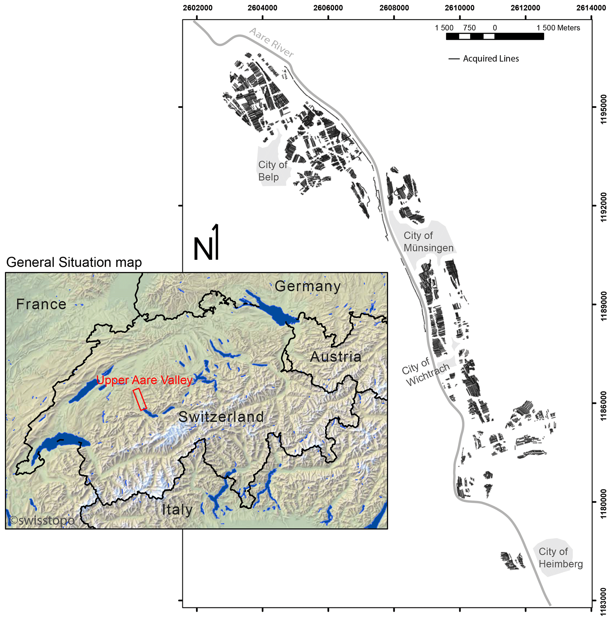
Figure 1 Location of the study area and acquisition lines. Coordinates are in UTM 32^∘ N (epsg: 32632).

Near-surface geophysics such as DC resistivity, electromagnetic, or seismic methods can bring important information in terms of the spatial distribution of facies. However, they are usually carried out in restricted areas to answer specific local questions and do not help to understand the variations in geology at the valley scale. In order to fill this gap of information, and provide a valley-scale fluvioglacial resistivity map, in January 2020 we conducted a large geophysical survey using a tTEM (towed transient electromagnetic) system (Auken et al., 2019) in the upper Aare Valley, Switzerland. The tTEM system provides a very detailed (both vertically and horizontally) resistivity model. The tTEM20AAR data set covers a section of the valley of approximately 1–2 km width and 16 km long. The fields were mapped with a line spacing of 20 m, resulting in about 1500 ha of covered land (see Fig. 1). The raw tTEM data were processed to suppress noisy data parts and then inverted to a resistivity model using spatially constrained inversion algorithm (Viezzoli et al., 2008). The resulting resistivity model consists of 57 862 1D models of 30 layers. The depth of investigation varies, from 40 to 120 m depth, primarily driven by lithological/resistivity variations. The resulting resistivity model explains (fits) the recorded data well within the estimated data uncertainty. The resistivity model reveals new and very interesting geophysical/geological structures of the subsurface at a fine resolution. At a first glance, they seem to reveal possible paleo river channels, various stages of glacial advances and retreat, and landslide lateral deposits. These structures still require a more detailed analysis and geological interpretation. Example of geological interpretations of such data are available in Sandersen et al. (2021).

Figure 2 The tTEM system.

The tTEM20AAR data set can be used for several purposes. It can be used as a benchmark to test and compare geophysical inversion procedures for tTEM systems. Stochastic inversion (Mosegaard and Tarantola, 1995; Linde et al., 2017) using different methods or types of prior knowledge could also be applied to this data set and be compared with the published results. In addition, if other geophysical data are acquired at the same site in the future, they could complement the analysis by performing joint inversion. More generally, quaternary formations are highly heterogeneous and constitute a challenge for geostatistical and uncertainty modeling (De Marsily et al., 2005). Sharing this data set will allow the testing and comparison of various methods to interpolate the properties of the underground and construct models that can be used for various purposes. The integration of geophysical methods to constrain hydrogeological models is also a very important field of research (Binley et al., 2015). The tTEM20AAR data set may help test the development of innovative methods for the construction of groundwater models. It is important to note in this perspective that the upper Aare Valley has been extensively studied, and a consequent amount of additional data is distributed by the Swiss authorities. Improvement in data integration may strongly improve hydrogeological modeling in such environments, subject to high local facies variations.

Finally, from a more geological perspective, the tTEM20AAR data set could be used to better understand the internal structures of quaternary deposits within alpine valleys. It could be analyzed in detail from a sedimentological perspective and used to better constrain the glacial and geological history of the quaternary deposits (Preusser et al., 2011).

2 Methods

2.1 The tTEM system

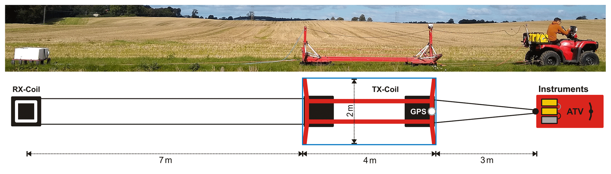
The tTEM system used for the data acquisition is developed by the HydroGeophysics Group (HGG) at Aarhus University, Denmark (Auken et al., 2019). The tTEM system is a towed, ground-based, transient electromagnetic system, designed for highly efficient data collection and detailed 3D mapping of the shallow subsurface (the upper ∼80 m). TEM methods build on the principle of induction (Faraday's law of induction) for mapping the electrical conductivity (conductivity =1 $/$ resistivity) of the subsurface. A detailed description of the TEM principle can be found in Christiansen et al. (2009). The layout of the tTEM system is shown in Fig. 2.

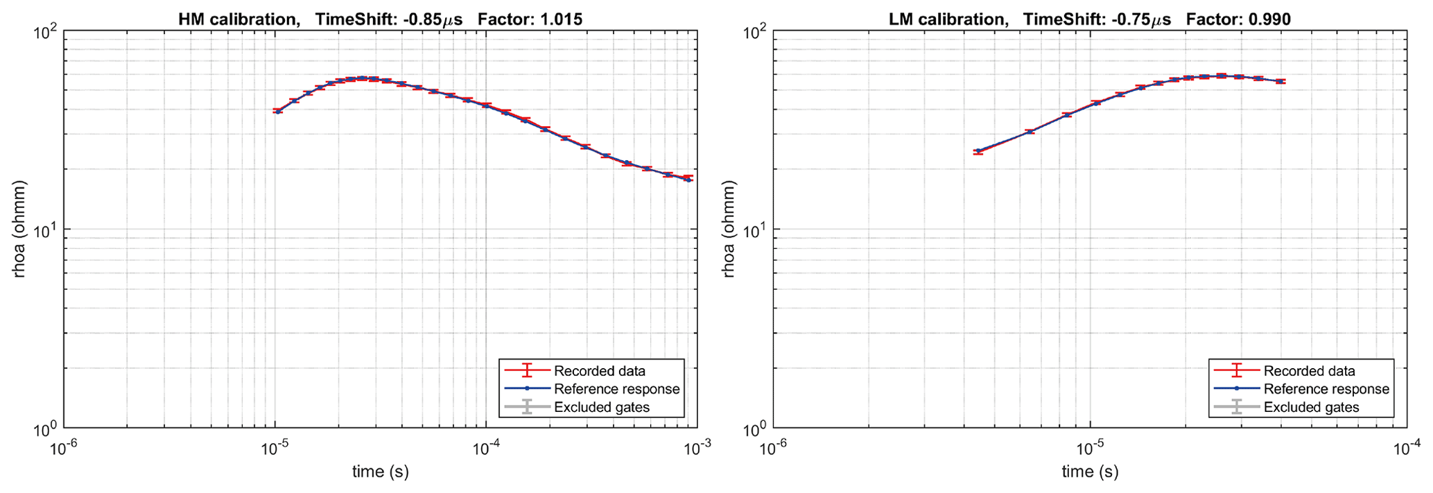
Figure 3 Calibration of the high and low moments. The resulting time shift and scale factor are respectively −0.75 µs and 0.99 for the LM and −0.85 µs and 1.015 for the HM.

The tTEM system consists of an all-terrain vehicle (ATV) carrying the instrumentation and towing the transmitter frame (Tx coil) and the receiver coil (Rx coil) in an offset configuration. The Tx and Rx coils are mounted on sleds for all terrain capability. All frame parts and sleds are built of non-conductive composite materials. Driving path and various data quality control parameters are monitored in real time by the driver on a mounted screen. Operation speed is up to 20 km/h. We used an off-set configuration, where the receiver coil is 7 m behind the transmitter coil. Both of them are horizontal, allowing the measurement of the z component of the secondary magnetic field. A GPS is mounted on the frame to ensure correct positioning of the data. The transmitter loop consists of one loop of 4×2 m, creating an area of 8 m². We used a standard dual-moment TEM configuration: a high moment (HM) with a high inductive current of 30 A and a low moment with a lower inductive current of 5 A. Such configuration has the advantage of being able to resolve shallow targets with the low moment and its associated fast turn off time and to reach higher penetration depth with the high moment. Both moments are stacked a few hundred times. Detailed parameters are summarized in Table 1. The gate is the time interval in which the received amplitudes are averaged. Due to the signal attenuation, the further we get in the listening time, lower the signal-to-noise ratio. In order to partially counterbalance this effect, we used a logarithmic increasing gate size related to listening time.

Table 1 Specifications of the high and low moment used in the acquisition. The gate size increases with time in order to counterbalance less good signal-to-noise ratio due to the wave attenuation.

To ensure the data quality, the tTEM instrumentation was calibrated prior to the survey at the Danish national TEM test site following the calibration procedure described by Foged et al. (2013). The two calibrated parameters are a time shift and an amplitude factor. The calibration was done with the ATV connected to the equipment in order to account for any shift caused by it. Figure 3 shows the match between the test site reference response and the measured tTEM response after calibration, which results in a fully acceptable match.

2.2 Field site

The field site is the upper Aare Valley, in central Switzerland (see Fig. 1). The survey took place in January 2020. During approximately 15 working days, we covered all the accessible farming fields in the valley along a 26 km long section. The driving speed was between 10 and 20 km/h, depending on the terrain. Since the acquisition rate is time dependant, and not distance triggered, we also lowered the speed in noisier or less responsive areas in order to acquire a denser data set. The spacing between the lines was approximately 20 m. The average covered surface par day was 112 ha, for a total of 1425 ha.

2.3 Data processing

The voltage data from the receiver is measured continuously and need to be cleaned of man-made noise and coupling. Data processing and inversion were carried out with the tTEM processing module in the Aarhus Workbench software. The objective of the processing of the tTEM data is to remove any interference in the data from man-made installation (coupled data), suppress random noise by stacking, and finally discard the noisy late time data entering the background noise. Thus, we ensure that the resulting resistivity model represents geological structures of the subsurface without artifacts from man-made installation. Processing of the $\mathrm{d}B/\mathrm{d}t$ data comprises the following steps.

• Automatic detection of capacitive coupling pattern in the raw data using a slope filter as coupling appears as abrupt slope changes in a sounding curve.

• Averaging of raw data to suppress random noise. Raw data are averaged using a moving-average filter with narrow time windows in early times and wider in the late times.

• Creation of vertical soundings every 2.5 s which corresponds approximately to a spacing of 10 m. The exact distance can vary depending on driving speed.

• Automatic filtering of the averaged data for removal of late-time data points entering the background noise.

• Visual assessment of all $\mathrm{d}B/\mathrm{d}t$ data and manual removal of coupled data not detected by the automatic filtering and validation of automatically detected couplings.

• Evaluation and adjustment of the data processing based on preliminary inversion results.

Furthermore GPS data are lag-corrected to geographical positioned data/models at center between transmitter and receiver coils. The data uncertainty consists of a minimum of 3 % as uniform data standard deviation (SD) plus the SD calculated from the data stacking. Averaged data resulting with SD over 30 % are discarded from the inversion.

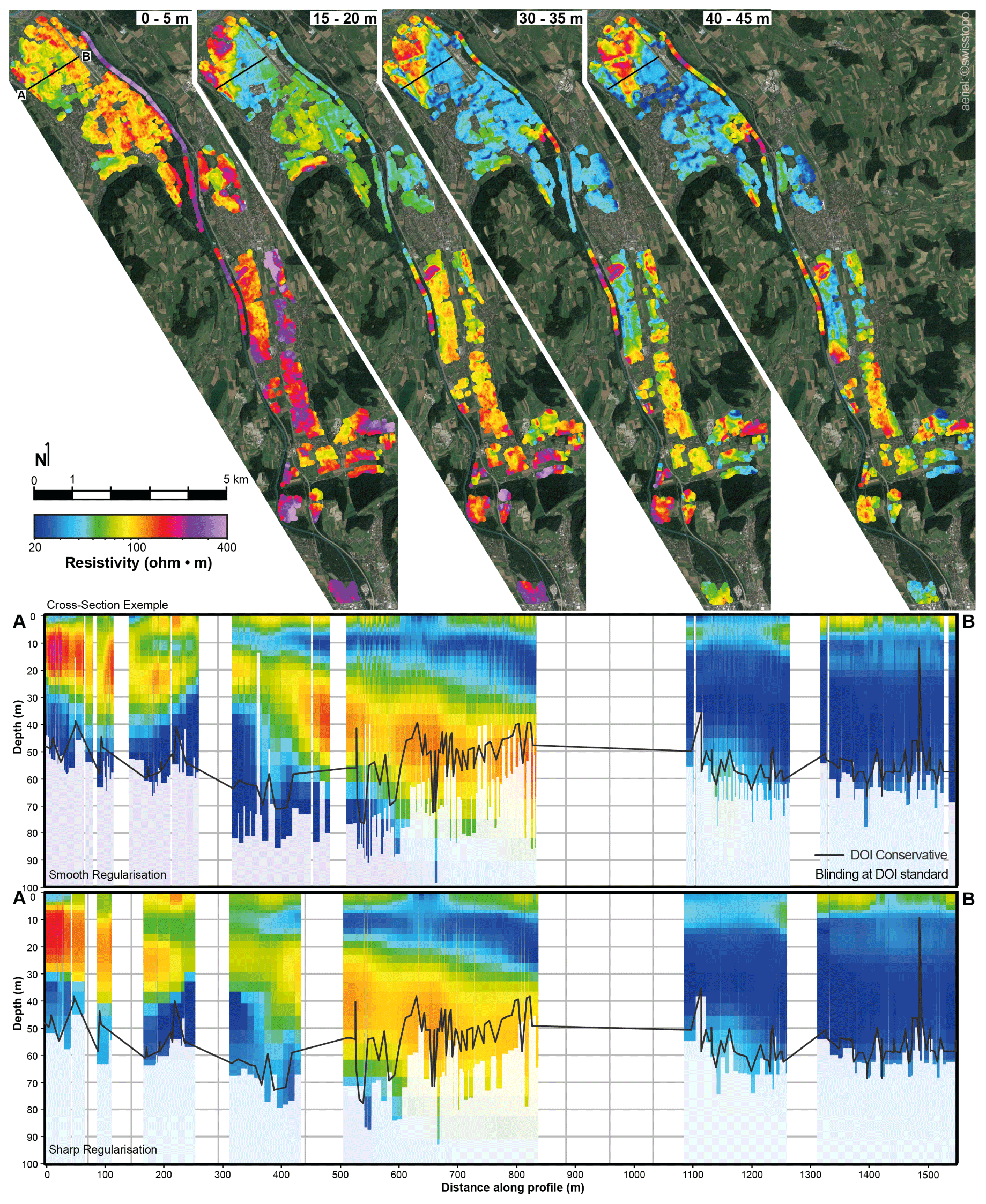
Figure 4 Top: mean resistivity maps at different depth intervals from the smooth regularization model. Bottom: NE–SW cross section with different regularizations. The models are blinded at the DOI standard, and the black line represents the DOI conservative.

Table 2 Settings used for the model setup and the smooth and the sharp regularization.

2.4 Inversion

The electrical resistivities of the underground are then estimated using a series of 3D constrained 1D inversions. The 1D inversion is based on the AarhusInv code (Auken et al., 2015; Kirkegaard et al., 2015). This code is an implementation of a 1D non-linear damped least-squares solution, with a modeled transfer function for the TEM instrumentation. This function takes into account the transmitter waveform, the instrument low-pass filters, the receiver bandwidth, the system geometry, the gate widths, and the instrument front gate. However, in such a stand-alone 1D inversion, each model is totally independent of the neighboring ones. To account for the lateral continuity expected in geological environments, the spatially constrained inversion (SCI) (Viezzoli et al., 2008) method was used. It applies 3D constraints to 1D inversion models both along and across the mapping lines, with a weight that is decreasing with distance. All the inversions were carried out with the Aarhus Workbench software.

The SCI inversion can be used with two different schemes of regularization: smooth or sharp. The smooth scheme tends to minimize abrupt changes in resistivity, in the vertical and horizontal directions. On the other hand, the sharp regularization scheme tends to minimize the number of resistivity changes but will consequently result in more abrupt resistivity transitions and a potentially more blocky model appearance. Both regularizations were used and are included in the output data.

For each resistivity model, we estimate the depth of investigation (DOI) using a method based on the Jacobian sensitivity matrix (Christiansen and Auken, 2012). This method has the advantage of taking into account the full transfer function, including system geometry, data uncertainty, and the resistivity model. Two DOI threshold values in the sensitivity matrix were used to provide the reported DOI standard and the DOI-conservative values. As a guideline, the resistivity structures above the DOI-conservative value are strongly data driven, while resistivity structures below the DOI-standard value are weakly represented in the data. Normally one would blank the resistivity models below the DOI-standard value. In addition, the shallowest resolution of the tTEM system is 2 to 3 m, depending on the resistivity.

Inversion setup for the smooth and sharp inversions is summarized in Table 2. Figure 4 presents some resistivity map data extracted from the smooth regularization inversion. In addition, the same cross section across the north area from the sharp and the smooth regularizations is displayed. Both DOIs are also outlined for comparison. The spatial variations of the Quaternary deposits, in both depth intervals and cross section are clearly visible. Such variations in resistivities also indicate variations in lithologies and therefore variations in hydrological proprieties.

3 Data records

After the data processing and the inversion, the processed data, the resistivity models and the associated forward responses from the smooth, and sharp inversions had been produced. These data (available at https://doi.org/10.5281/zenodo.4269887; Neven et al., 2020) are provided in column-based ASCII files. Each file structure is outlined in the following sections.

3.1 Processed data file

The Processed_Data.dat file contains the processed tTEM data and data uncertainties. Each line in the file corresponds to a low-moment (LM) or high-moment (HM) data stack for a given location. The RECORD number links the LM and HM data to a given resistivity model in the *.inv files. Number 9999 marks discarded data points or data points not present for the given moment. If all the data points of LM or HM are discarded, then the data line is not present in the file. Gate center time and other info are stated in the header lines. The data uncertainty is given as relative in log space. The upper and lower bounds of the data are then defined as

$$\begin{array}{}\text{(1)}& {\displaystyle }{\text{unc}}_{\text{down}}={\displaystyle \frac{\text{DATA}}{\mathrm{1}+\text{DATASTD}}},\text{(2)}& {\displaystyle }{\text{unc}}_{\text{up}}=\text{DATA}\times (\mathrm{1}+\text{DATASTD}),\end{array}$$

with unc_down and unc_up being the absolute lower and upper uncertainties, DATA the processed z component $\mathrm{d}B/\mathrm{d}t$ data value, and DATASTD the relative uncertainty. The structure is outlined in the following Table 3.

Table 3 Structure of the .dat data file.

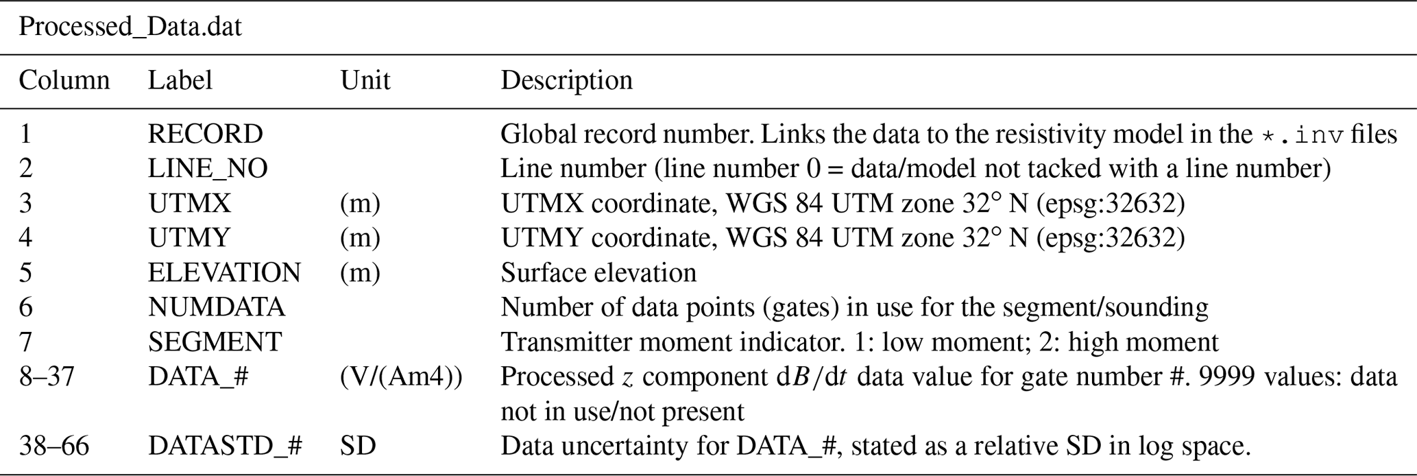
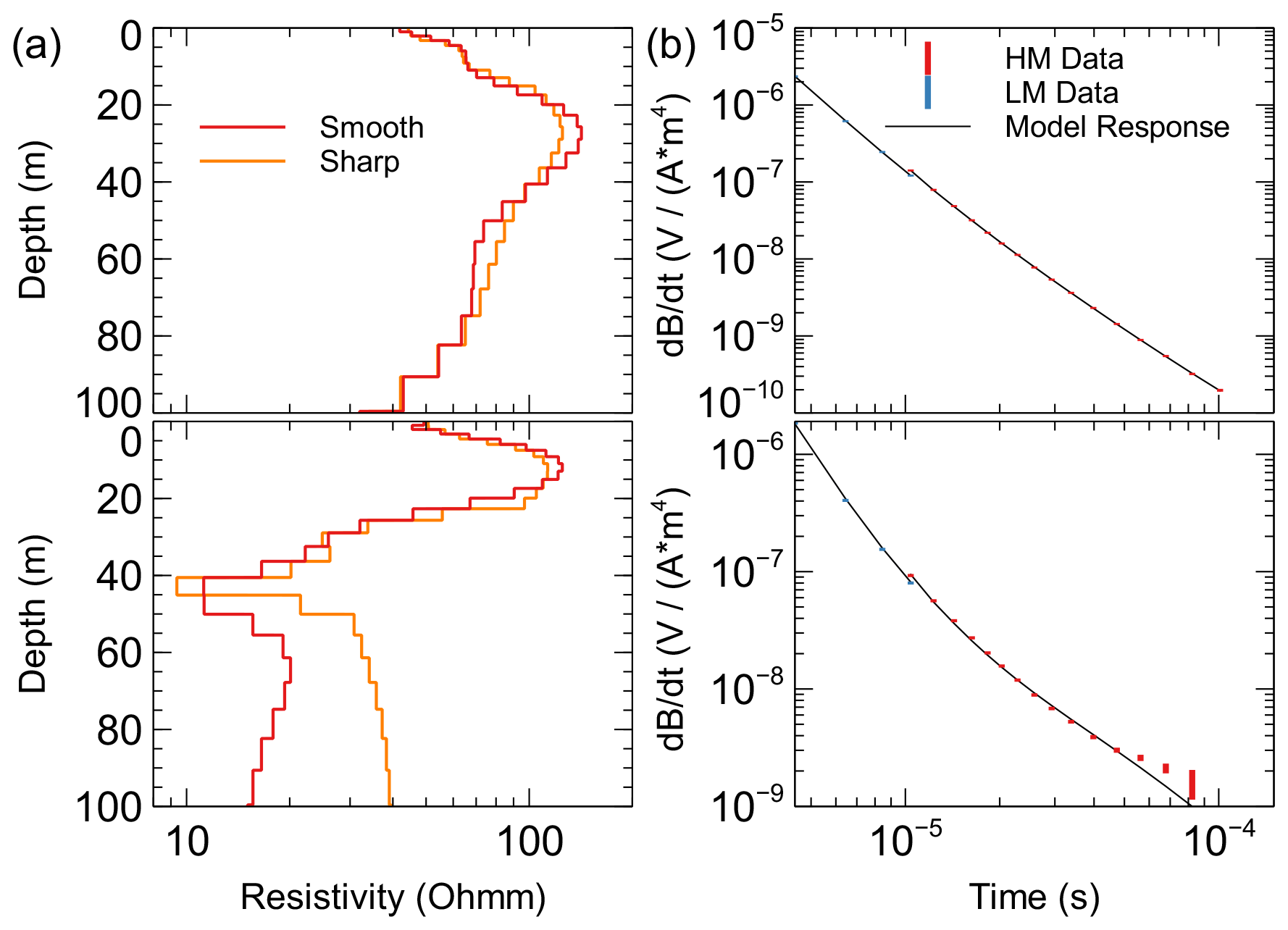
Figure 5 Example of two 1D models at a location, with the top one considered to be undisturbed and the bottom one to be a noisy sounding. Top: number 44384 on line 20350 at position 384744.1875/5196856 UTM 32 N. Bottom: number 38407 on line 17610 at position 384313/5195797. (a) Resistivity models for two regularizations. (b) Associated forward response of the smooth model in black, with the LM and HM data points with red and blue error bars. The normalized data fit (see text) for the top model–data curve is 0.27 and 1.36 for the bottom model.

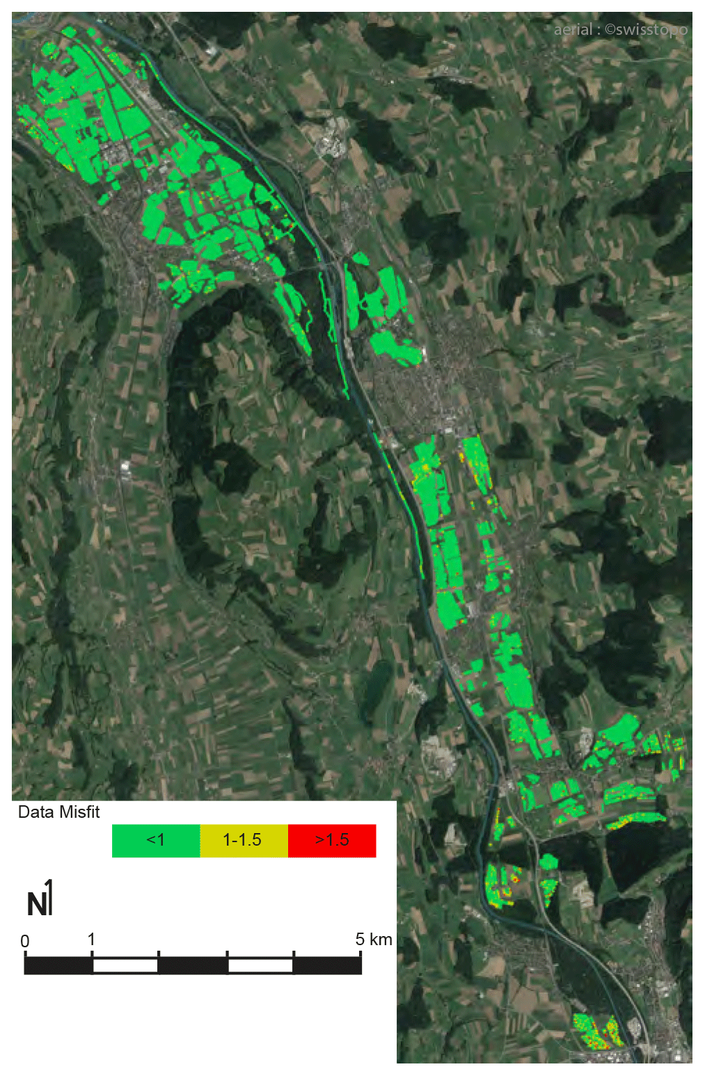
Figure 6 Data misfit over the acquisition area. Base map from Swiss Federal Topographic Office.

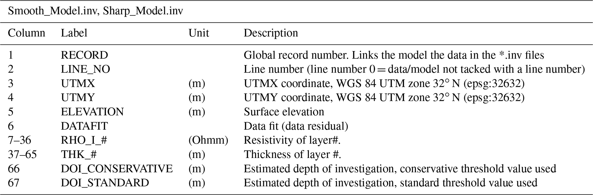
3.2 Inversion model file

The Sharp_Model.inv and Smooth_Model.inv files contain the resistivity models (layer resistivity and layer thicknesses). Each line holds a 30-layer resistivity model. The RECORD links the model to the data in the process data and forward data files. The file also contains the DOI and the data fit. Note that the last layer (layer 30) does not have a thickness since it continues to infinite depth in the modeling. Normally, the DOI-standard values are used to blank the models in depths. The detailed file structure is provided in Table 4.

Table 4 Structure of the *.inv data file.

3.3 Synthetic response file

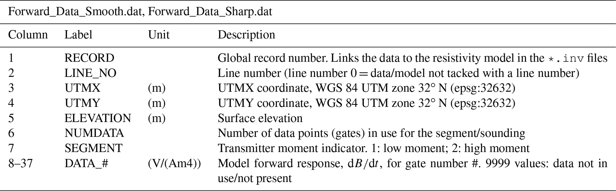
The Forward_Data_Sharp.dat and Forward_Data_Smooth.dat files contain the forward responses of the sharp and smooth resistivity models. The structure of the forward data files is the same as the Processed_Data.dat file except that the forward responses do not have associated data uncertainties. Detailed file structure is provided in Table 5.

Table 5 Structure of the *.syn data file.

4 Code availability

All the data importation, processing, and SCI inversions were done using Aarhus Workbench commercial software developed by Aarhusgeosoftware. The 1D inversion code used is AarhusInv developed by the Aarhus University Hydrogeophysics group (Auken et al., 2015; Kirkegaard et al., 2015). The AarhusInv code is free to use for research purposes.

5 Data availability

The data (syn, dat, and inv) are provided in column-based ASCII files and are available at https://doi.org/10.5281/zenodo.4269887 (Neven et al., 2020).

6 Technical validation

After the removal of coupled structures, the main indicator of geophysical data quality is the fit with the inverted model. In the case of error in the data, such as undetected coupling for example, the data will not be fitted by any plausible resistivity model and will present an important residual error. Therefore, a good fit between the theoretical forward response and the field data indicates that the data are representative of the geology and not affected by errors or noise.

The quality of inversion is assessed by a quality control parameter called data misfit. We compare the forward geophysical response of our final resistivity model with the field data, normalized by the square of the standard deviation of our data. The indicator is defined by the following Eq. (3).

$$\begin{array}{}\text{(3)}& \text{Data misfit}=\sqrt{{\displaystyle \frac{\mathrm{1}}{N}}\sum _{i=\mathrm{1}}^N{\displaystyle \frac{(d_{\mathrm{obs},i}-d_{\mathrm{frw},i}{)}^{\mathrm{2}}}{{\mathit{\sigma }}_{\mathrm{d},i}^{\mathrm{2}}}}},\end{array}$$

where d_obs is the observed data, d_fwr is the forward data, σ_d is the uncertainty of the observed data, and N is the total number of data points.

A data residual below 1 indicates that our final model response is within 1 standard deviation of the data, when a value above 1 indicates a response out of 1 standard deviation. Figure 5b shows a single data curve (error bars) and the forward response (line) from the resistivity models in Fig. 5a. Both regularizations are shown. The first model (top subfigure) is situated in the middle of a field, when the second model (bottom subfigure) is close to a road, which is a typical source for electromagnetic noise. The associated data misfit for the first model is 0.27 and 1.36 for the noisier one. Most of the misfit comes from the latest's gates, when the signal-to-noise ratio is getting small. The data misfit for the all-smooth inversion models is plotted in Fig. 6. As seen in Fig. 6, the data misfit is in general well below one and fully acceptable. A total of 95 % of the data is within 1 standard deviation, with a global misfit average of 0.65 and 0.52 respectively for the sharp and smooth models. A manual inspection of the high-data-misfit models revealed that they are all associated with highly resistive models and/or are close to man made electromagnetic noise such as roads, fences, or train tracks. A good example is the extreme south of the acquisition, which is one of the most resistive areas. This situation logically leads to a lower signal-to-noise ratio, and due to the spatial constraints of the inversion, it will consequently lead to a higher data misfit. However, they are usually restricted to only a few local data points, and the models are similar to neighboring ones that have acceptable misfit. We therefore decided to keep them in the data set.

Finally, users of the data should be aware that the footprint of the equipment is at least 9 m at the surface (size of the equipment) and is increasing with depth and wave diffusion. Consequently, a sharp vertical transition in the geology, for example, will tend to appear oblique in the resistivity data due to this effect. The resistivity model proposed here is only the one that fits our data the best.

Usage notes

Since the file data format is a standard ASCII file, all the files can be used with any program supporting xyz format.