Integrated water vapour observations in the Caribbean arc from a network of ground-based GNSS receivers during EUREC⁴A

Ground-based Global Navigation Satellite System (GNSS) measurements from nearly 50 stations distributed over the Caribbean arc have been analysed for the period 1 January–29 February 2020 in the framework of the EUREC⁴A (Elucidate the Couplings Between Clouds, Convection and Circulation) field campaign. The aim of this effort is to deliver high-quality integrated water vapour (IWV) estimates to investigate the moisture environment of mesoscale cloud patterns in the trade winds and their feedback on the large-scale circulation and energy budget.

This paper describes the GNSS data processing procedures and assesses the quality of the GNSS IWV retrievals from four operational streams and one reprocessed research stream which is the main data set used for offline scientific applications. The uncertainties associated with each of the data sets, including the zenith tropospheric delay (ZTD)-to-IWV conversion methods and auxiliary data, are quantified and discussed. The IWV estimates from the reprocessed data set are compared to the Vaisala RS41 radiosonde measurements operated from the Barbados Cloud Observatory (BCO) and to the measurements from the operational radiosonde station at Grantley Adams International Airport (GAIA), Bridgetown, Barbados. A significant dry bias is found in the GAIA humidity observations with respect to the BCO sondes (−2.9 kg m⁻²) and the GNSS results (−1.2 kg m⁻²). A systematic bias between the BCO sondes and GNSS is also observed (1.7 kg m⁻²), where the Vaisala RS41 measurements are moister than the GNSS retrievals. The IWV estimates from a collocated microwave radiometer agree with the BCO soundings after an instrumental update on 27 January, while they exhibit a dry bias compared to the soundings and to GNSS before that date. IWV estimates from the ECMWF fifth-generation reanalysis (ERA5) are overall close to the GAIA observations, probably due to the assimilation of these observations in the reanalysis. However, during several events where strong peaks in IWV occurred, ERA5 is shown to significantly underestimate the GNSS-derived IWV peaks. Two successive peaks are observed on 22 January and 23–24 January which were associated with heavy rain and deep moist layers extending from the surface up to altitudes of 3.5 and 5 km, respectively. ERA5 significantly underestimates the moisture content in the upper part of these layers. The origins of the various moisture biases are currently being investigated.

We classified the cloud organization for five representative GNSS stations across the Caribbean arc using visible satellite images. A statistically significant link was found between the cloud patterns and the local IWV observations from the GNSS sites as well as the larger-scale IWV patterns from the ECMWF ERA5 reanalysis.

The reprocessed ZTD and IWV data sets from 49 GNSS stations used in this study are available from the French data and service centre for atmosphere (AERIS) (https://doi.org/10.25326/79; Bock, 2020b).

1 Introduction

The overarching goal of EUREC⁴A (Elucidate the Couplings Between Clouds, Convection and Circulation) is to improve our understanding of how trade-wind cumuli interact with the large-scale environment (Bony et al., 2017). Water vapour is one key ingredient of the atmospheric environment controlling the life cycle of convection with strong feedback on the large-scale circulation and energy budget (Sherwood et al., 2010). The mechanisms involved are thought to play a significant role in the climate sensitivity and model diversity (Sherwood et al., 2014).

The EUREC⁴A field campaign was elaborated to provide relevant observations on the cloud properties and their atmospheric and oceanic environment across a range of scales (Stevens et al., 2021). The measurement platforms were deployed over two theatres of action. The first, referred to as the “Tradewind Alley”, extends from an open-ocean mooring at 50.95^∘ W, 14.74^∘ N to the Barbados Cloud Observatory (BCO) (59.43^∘ W, 13.16^∘ N) (Stevens et al., 2016). The second, named the “Boulevard des Tourbillons”, extends from 7^∘ N, off the northern Brazil coast, roughly to the BCO. Most of the distant open-seawater vapour measurements were made by research vessels (R/Vs) embarking radiosonde systems, lidars, and microwave radiometers for what concerns water vapour measurements. They were completed by aircraft platforms leaving from the Grantley Adams International Airport (GAIA), Brigdetown, Barbados, embarking dropsondes, in situ, and remote sensing measurement systems. The aircraft operated mainly in a 200 km diameter circle centred on 57.72^∘ W, 13.32^∘ E in the Tradewind Alley, upstream from the BCO. In addition to the research instrumentation deployed on these platforms, ground-based and ship-borne Global Navigation Satellite System (GNSS) receivers were operated to provide high-temporal-resolution integrated water vapour (IWV) measurements. Results of ship-borne GNSS measurements from the R/Vs Meteor, Maria S. Merian, and L'Atalante are described in a companion paper (Bosser et al., 2021). This paper focuses on the ground-based GNSS network measurements.

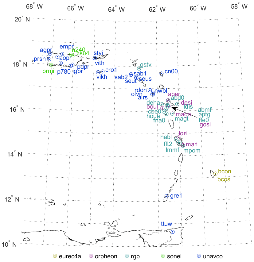
Figure 1 Map of GNSS stations for which the measurements were reprocessed from 1 January to 29 February 2020. The data sources are indicated below the figure.

The ground-based GNSS network comprises a total of 49 stations of which 47 are permanent instruments devoted primarily to geoscience investigations. Most of these stations belong to the Continuously Operating Caribbean GPS Observational Network (COCONet) (https://coconet.unavco.org/, last access: 29 January 2021) and provide raw observations as well as station positions and velocities for monitoring, understanding, and prediction of various geohazards (earthquakes, hurricanes, flooding, volcanoes, and landslides). Some other stations belong to the French permanent GNSS network, the so-called “Reseau GNSS Permanent” (RGP) operated by IGN in the Caribbean and French Guyana territories. Figure 1 shows the map of the stations. Because of their location on the nearby Caribbean islands, most of the GNSS measurements mainly provide information on the large-scale atmospheric environment downstream the Tradewind Alley and the Boulevard des Tourbillons. Closer to the main theatre of action of the field campaign, two collocated ground-based GNSS stations, referred to as BCON and BCOS, have been set up at the BCO in the framework of EUREC⁴A. Two stations were installed to insure redundancy during the campaign. They complement the permanent instrumentation operated at the BCO (Stevens et al., 2016). The BCO GNSS stations were installed on 31 October 2019 and are planned to operate for a full annual cycle at least. The measurements from these two stations are transmitted in near-real time thanks to the BCO infrastructure and are processed operationally by IGN in the RGP processing stream, on one hand, and by ENSTA_B/IPGP (ENSTA Bretagne and IPGP), on the other hand. Both processing centres run continuously and provide IWV data with slightly different latency and precision. A more accurate research-mode processing was also set up by ENSTA_B/IPGP to reprocess the data from all 49 stations in a homogeneous way but for a limited period, from 1 January to 29 February 2020, hence including the COCONet and RGP stations. A first release of this data set is now available on the EUREC⁴A database hosted by the French data and service centre for atmosphere (AERIS) (Bock, 2020b).

This paper aims at describing the ground-based GNSS data processing details and assessing the quality of the IWV retrievals from both the operational and research processing streams. Section 2 describes the GNSS data processing and IWV conversion details. Section 3 compares the zenith tropospheric delay (ZTD) estimates and the IWV retrievals from the various data processing streams for the two BCO stations. The intercomparison is completed with IWV measurements from the Vaisala RS41 radiosondes and the humidity and temperature profiler (HATPRO) microwave radiometer operated during the EUREC⁴A campaign, as well the operational radiosonde measurements operated by the Barbados weather service at GAIA. Section 4 provides a validation of the ECMWF fifth-generation reanalysis (ERA5) (Hersbach et al., 2020) at regional scale with respect to the IWV retrievals from the extended GNSS network and a preliminary analysis of the large-scale IWV variations related to mesoscale cloud organization in the trade winds. Section 5 concludes the study.

2 GNSS data processing and IWV retrieval

A vast literature covers the basic concepts of GNSS data processing for meteorological applications (see Guerova et al., 2016). It will not be repeated here.

2.1 GNSS data processing streams

The GNSS measurements from the two BCO stations, hereafter called BCON and BCOS, are processed in four different operational streams. Two of the streams are run by IGN as part of the RGP operations that will be referred to as “RGP NRT” (near-real time) and the “RGP daily”. Both consist in network processing solutions where the BCO stations are processed in baselines formed with about 40 permanent stations operated in the Caribbean and French Guyana region and beyond. The processing results, hereafter called “solutions”, are produced on hourly and daily basis, respectively. The NRT solution uses ultra-rapid satellite clocks and orbits, and processes the measurements in 6-hourly windows shifted by 1 h every hour. For the permanent GNSS stations in the region, the ZTD estimates for the most recent hour are available within 45 min after the end of measurements and are distributed to numerical weather prediction (NWP) centres via the EUMETNET-GNSS water vapour programme (E-GVAP). Although the BCO stations were included in this stream, they are not registered as permanent stations at E-GVAP and are thus not assimilated by the NWP centres. Due to the sliding window processing approach, each hourly time slot is thus processed six times. The accuracy of the corresponding ZTD estimates depends on the time slot, as will be illustrated in the next section. The main reason is that the quality of the NRT clocks and orbits is lower in the more recent time slot because they are predicted (observations are not available in due time to constrain that part of the orbit calculation). The sampling of the ZTD estimates of the NRT solution is 15 min. On the other hand, the “daily” processing stream is updated every day before 05:00 UTC. It is based on a longer time window of 24 h and benefits from slightly improved clock and orbit products. Its accuracy is thus slightly higher. The sampling of the ZTD estimates of the daily solution is 1 h. This processing stream is not sent to E-GVAP but is rather devoted to an operational quality control of the observations from the RGP stations. It is also used for a posteriori verification of the NRT solution.

The data from the BCO stations were also included in two other operational streams operated by ENSTA_B/IPGP in the framework of ACTRIS-France (Aerosol, Cloud and Trace Gases Research Infrastructure – France, https://www.actris.fr/, last access: 29 January 2021). These two streams are referred to as “GIPSY rapid” and “GIPSY final”. They differ only by the clock and orbit products which are released with daily and fortnightly latency, respectively. The GIPSY rapid processing is equivalent to the RGP daily processing, while the GIPSY final processing provides a higher level of accuracy. Both streams provide ZTD estimates with a sampling of 5 min.

Bar-Sever et al. (1998)Bertiger et al. (2010)

Table 1 Details of the five processing streams operated by IGN and ENSTA_B/IPGP in the framework of EUREC⁴A.

Apart from the usage of different clock and orbit products, the processing streams run by both analysis centres also differ by their software packages and related processing options as summarized in Table 1. Most importantly, IGN uses the Bernese GNSS version 5.2 software in double-difference processing mode (Dach et al., 2015), while ENSTA_B/IPGP use the GIPSY OASIS II version 6.2 software in precise point positioning (PPP) mode (Zumberge et al., 1997). Various studies have compared the results and discussed the benefits and drawbacks of both approaches. When consistent clock and orbit products are used, there is generally a good level of agreement (i.e. a few millimetres of root mean square differences (RMSDs) in ZTD estimates).

Finally, the regional network including 49 GNSS stations was reprocessed by ENSTA_B/IPGP using again GIPSY OASIS II version 6.2 software, in a very similar scheme to that of the final stream but with a few improved processing options. This processing is expected to be the most accurate. It is referred to as “GIPSY repro1” in the following.

2.2 GNSS data quality checking

The quality of the data processing results can be checked with two types of information: (1) global information quantifying the accuracy of the processing in the 6-hourly or 24-hourly time window (e.g. reduced sum of squares of residuals, percentage of solved ambiguities) and (2) the formal errors of the estimated parameters (station coordinates and ZTDs).

For the operational streams, only the second type of information was available, and a basic screening procedure was thus applied in the form of a range check on ZTD estimates with limits [1, 3 m] and on for ZTD formal errors with a limit of 0.02 m.

For the GIPSY repro1 solution, a more elaborate quality check was made using both types of information for all stations. Mean statistics over the 2-month period are reported in Table S1 of the Supplement. The mean rms of residuals for all 49 stations ranged between 0.009 and 0.015 m. Five stations with values above 0.013 m may be unreliable (N240, DEHA, AIRS, BOUL, HABL). These stations also have a small mean percentage of fixed ambiguities (≤50 %) and/or significant temporal variations in both parameters. Station position repeatability was in general good both in the horizontal (≤0.005 m) and vertical (≤0.015 m) except for two stations (BOUL, OLVN). In a second step, a tighter range check completed with an outlier check were applied following the recommendations of Bock (2020a). The range check limits were [0.5, 3.0 m] on ZTD values and 0.01 m on formal errors. The outlier check limits were computed for each station based on its median μ and standard deviation σ statistics over the 2-month period according to $[\mathit{\mu }-\mathrm{5}\mathit{\sigma },\mathit{\mu }+\mathrm{5}\mathit{\sigma }]$ for the ZTD values and $[\mathrm{0},\mathit{\mu }+\mathrm{3.5}\mathit{\sigma }]$ for the formal errors. This screening procedure rejected 0.21 % of the ZTD data due exclusively to the formal error outlier check. The GIPSY ZTD time series are generally quite small with few outliers as confirmed by the low outlier detection rate.

2.3 GNSS ZTD-to-IWV conversion

The ZTD is the sum of the zenith hydrostatic delay (ZHD) and the zenith wet delay (ZWD):

$$\begin{array}{}\text{(1)}& \text{ZTD}=\text{ZHD}+\text{ZWD}.\end{array}$$

During the data processing, ZHD is fixed to an a priori value, either from an empirical model or from a NWP model analysis (Boehm et al., 2007), and ZWD is estimated. Errors in the a priori ZHD can propagate to the estimated ZWD, but in general, this error is small (<1 mm) and the sum of both is very close to the real ZTD. When IWV is to be extracted, it is desirable to use a more accurate ZHD value computed from the surface air pressure:

$$\begin{array}{}\text{(2)}& \text{ZHD}={\mathrm{10}}^{-\mathrm{6}}{k}_{\mathrm{1}}{R}_{\mathrm{d}}{\displaystyle \frac{P_{\mathrm{s}}}{g_{\mathrm{m}}}},\end{array}$$

where k₁ is the dry air refractivity coefficient, R_d the dry air specific gas constant, P_s surface air pressure, and g_m the mean acceleration due to gravity (Davis et al., 1985). IWV is derived from ZWD by applying a delay to mass conversion factor κ(T_m):

$$\begin{array}{}\text{(3)}& \text{IWV}=\mathit{\kappa }\left(T_{\mathrm{m}}\right)\times \text{ZWD}.\end{array}$$

κ is a semi-empirical function of the weighted mean temperature T_m defined as (Bevis et al., 1992)

$$\begin{array}{}\text{(4)}& \mathit{\kappa }\left(T_{\mathrm{m}}\right)={\displaystyle \frac{{\mathrm{10}}^{\mathrm{6}}}{R_{\mathrm{v}}\left(k_{\mathrm{2}}^{\prime }+\frac{k_{\mathrm{3}}}{T_{\mathrm{m}}}\right)}},\end{array}$$

where $k_{\mathrm{2}}^{\prime }$ and k₃ are refractivity coefficients for the water molecule; R_v is the specific gas constant for water vapour. T_m is defined as

$$\begin{array}{}\text{(5)}& T_{\mathrm{m}}={\displaystyle \frac{\int {\mathit{\rho }}_{\mathrm{v}}\left(z\right)\mathrm{d}z}{\int \frac{{\mathit{\rho }}_{\mathrm{v}}\left(z\right)}{T\left(z\right)}\mathrm{d}z}},\end{array}$$

where ρ_v(z) and T(z) and the specific mass of water vapour and the air temperature, respectively, at height z above the surface. The integrals are from the surface to the top of the atmosphere.

Practically, the GNSS IWV estimates are converted from the ZTD data using Eqs. (1) to (4) with the auxiliary data, P_s and T_m, given at the position of the GNSS station with interpolation to the GNSS times. On average, for the 2-month period (January–February 2020), the conversion parameter amounts to $\stackrel{\mathrm{‾}}{\mathit{\kappa }}=\mathrm{164}$ kg m⁻³ and the observed $\stackrel{\mathrm{‾}}{\text{ZWD}}=\mathrm{0.20}$ m results into $\stackrel{\mathrm{‾}}{\text{IWV}}=\mathrm{32}$ kg m⁻². The sensitivity of IWV estimates to errors in the auxiliary data can be assessed by the partial derivatives: $\frac{\partial \text{IWV}}{\partial \text{ZTD}}=-\frac{\partial \text{IWV}}{\partial \text{ZHD}}=\mathrm{0.16}$ (kg m⁻²) mm⁻¹, and $\frac{\partial \text{IWV}}{\partial \mathit{\kappa }}=\mathrm{0.20}$ (kg m⁻²) (kg m⁻³)⁻¹, or equivalently $\frac{\partial \text{IWV}}{\partial P_{\mathrm{s}}}=\mathrm{0.35}$ (kg m⁻²) hPa⁻¹ and $\frac{\partial \text{IWV}}{\partial T_{\mathrm{m}}}=\mathrm{0.12}$ (kg m⁻²) K⁻¹, where the numerical values were computed from the average EUREC⁴A conditions.

Various sets of refractivity coefficients and auxiliary data were available and used with our operational and research GNSS products and are described in the subsections below.

2.3.1 RGP NRT and daily results

This data set is provided only for the BCON and BCOS stations which benefit from collocated surface air pressure and temperature measurements. The measurements come from Vaisala PTU200 sensors connected directly to the GNSS receivers and are included in the raw GNSS data files. The ZHD estimates are therefore computed using Eq. (2) and the T_m values are computed using the widely used Bevis et al. (1992) formula:

$$\begin{array}{}\text{(6)}& T_{\mathrm{m}}=\mathrm{70.2}+\mathrm{0.72}{T}_{\mathrm{s}},\end{array}$$

where T_s is the surface pressure. This formula was derived by Bevis et al. (1992) from a radiosonde data set over the US with a root mean square error (RMSE) of 4.7 K. The refractivity coefficients used for the computation of ZHD and κ are from Thayer (1974), the thermodynamics constants are from ICAO (1993), and the g_m formula is from Saastamoinen (1972).

2.3.2 GIPSY rapid and final results

This data set is also provided only for the BCON and BCOS stations but it used the a priori values for ZHD available during the data processing. The values were obtained from the Technical University of Vienna (TUV) as part of the VMF1 tropospheric parameters computed from the ECMWF operational analysis (Boehm et al., 2006). The TUV also computes T_m values using Eq. (5) from the same analysis. Both products are made available on a global grid with 2^∘ latitude and 2.5^∘ longitude resolution every 6 h. The refractivity coefficients and g_m are the same as those for the RGP data set.

2.3.3 GIPSY repro1 results

For the reprocessed data set, we used a more rigorous approach following Bock (2020a). Here, the ZHD and T_m values are computed from ERA5 pressure-level data at the four surrounding grid points and are interpolated bilinearly to the positions of the GNSS antennas. The ERA5 fields were used with the highest temporal and spatial resolutions: 1-hourly and 0.25^∘ × 0.25^∘, respectively. The refractivity coefficients and thermodynamics constants were updated from Bock (2020a) to account for the global CO₂ content for January 2020 (see the Appendix). The g_m formula proposed by Bosser et al. (2007) was used instead of the Saastamoinen (1972) one.

This methodology provides the most accurate IWV estimates regarding the available data at the 49 stations of the extended network and the best knowledge of uncertainties due to the various empirical formulas (T_m and g_m) and auxiliary data.

2.3.4 Uncertainty due to IWV conversion methods

The three data sets (RGP, GIPSY operational, and GIPSY repro1) used different conversion methods, which are associated with different uncertainties. Although repro1 is the most accurate, it is not an operational stream and covers only a limited period of time. Users may thus be interested in the near-real-time and extended time coverage of the two operational data sets available for stations BCON and BCOS. The consistency of the different data sets is assessed in the next section for ZTD and IWV. Here, we describe how the different error sources contribute to overall uncertainty in the IWV data.

Let us consider two ZTD solutions from two different processing streams, ZTD₁ and ZTD₂, converted to IWV using different ZHD and κ data, ZHD_1,2 and κ_1,2. The two IWV solutions (IWV₁ and IWV₂) write

$$\begin{array}{}\text{(7)}& {\displaystyle }{\text{IWV}}_{\mathrm{1}}={\mathit{\kappa }}_{\mathrm{1}}\cdot ({\text{ZTD}}_{\mathrm{1}}-{\text{ZHD}}_{\mathrm{1}})\text{(8)}& {\displaystyle }{\text{IWV}}_{\mathrm{2}}={\mathit{\kappa }}_{\mathrm{2}}\cdot ({\text{ZTD}}_{\mathrm{2}}-{\text{ZHD}}_{\mathrm{2}}).\end{array}$$

The difference $\mathrm{\Delta }\text{IWV}={\text{IWV}}_{\mathrm{2}}-{\text{IWV}}_{\mathrm{1}}$ can be separated into systematic and random components and written as a function of the contributions (assumed independent) of the systematic and random differences of the three parameters $\mathrm{\Delta }\text{ZTD}={\text{ZTD}}_{\mathrm{2}}-{\text{ZTD}}_{\mathrm{1}}$, $\mathrm{\Delta }\text{ZHD}={\text{ZHD}}_{\mathrm{2}}-{\text{ZHD}}_{\mathrm{1}}$, $\mathrm{\Delta }\mathit{\kappa }={\mathit{\kappa }}_{\mathrm{2}}-{\mathit{\kappa }}_{\mathrm{1}}$ as

$$\begin{array}{}\text{(9)}& {\displaystyle }\stackrel{\mathrm{‾}}{\mathrm{\Delta }\text{IWV}}={\mathit{\kappa }}_{\mathrm{2}}\cdot \stackrel{\mathrm{‾}}{\mathrm{\Delta }\text{ZTD}}-{\mathit{\kappa }}_{\mathrm{2}}\cdot \stackrel{\mathrm{‾}}{\mathrm{\Delta }\text{ZHD}}+{\displaystyle \frac{{\text{IWV}}_{\mathrm{1}}}{{\mathit{\kappa }}_{\mathrm{1}}}}\stackrel{\mathrm{‾}}{\mathrm{\Delta }\mathit{\kappa }}\text{(10)}& {\displaystyle }\begin{array}{rl}({\mathit{\sigma }}_{\mathrm{\Delta }\text{IWV}}{)}^{\mathrm{2}}& =({\mathit{\kappa }}_{\mathrm{2}}\cdot {\mathit{\sigma }}_{\mathrm{\Delta }\text{ZTD}}{)}^{\mathrm{2}}+({\mathit{\kappa }}_{\mathrm{2}}\cdot {\mathit{\sigma }}_{\mathrm{\Delta }\text{ZHD}}{)}^{\mathrm{2}}\\ & +{\left({\displaystyle \frac{{\text{IWV}}_{\mathrm{1}}}{K_{\mathrm{1}}}}{\mathit{\sigma }}_{\mathrm{\Delta }\mathit{\kappa }}\right)}^{\mathrm{2}}.\end{array}\end{array}$$

The magnitude of the actual errors in the auxiliary data used in the different conversion methods can be determined from Fig. 2. The figure shows that the ZHD data computed from ERA5 reanalysis and PTU sensor agree well. The mean pressure (ZHD) difference (ERA5 − PTU) amounts to $-\mathrm{0.13}\pm \mathrm{0.20}$ hPa ($-\mathrm{0.30}\pm \mathrm{0.45}$ mm), whose impact on IWV represents 0.045±0.070 kg m⁻². ERA5 is thus a good source of surface pressure for the IWV conversion with negligible bias at this site. The ZHD estimates computed from ECMWF by TUV on the other hand have significant aliasing errors (Fig. 2). This is due to the strong atmospheric tide seen in the surface pressure that cannot be resolved by the 6-hourly analysis data (shown by crosses upon the dashed red line in the lower ZHD panel).

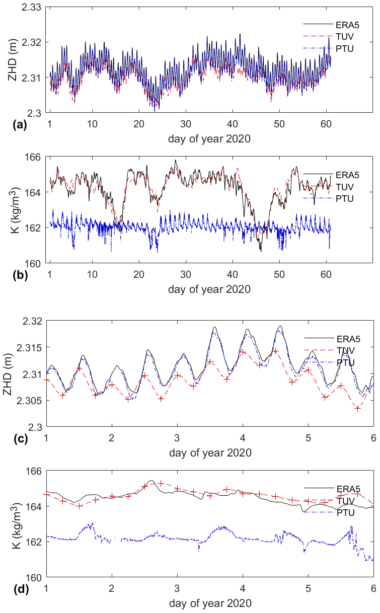
Figure 2 Time series of the auxiliary data (ZHD and K) used to convert ZTD to IWV in the different GNSS streams: high-resolution ERA5 pressure-level data, ECMWF analysis provided by TUV, surface pressure and temperature observations (PTU) for GNSS station BCON (a, b) from 1 January to 29 February 2020 and (c, d) from 1 to 6 January 2020.

Regarding the κ data, TUV and ERA5 agree well but the PTU-derived curve has significant errors because it uses the empirical formula given by Eq. (6) which is based on surface temperature and does not correlate well with the upper air variations that influence T_m. In the case of the RGP data set, the use of the Bevis et al. (1992) formula is the dominant error source in the IWV conversion process, while in the case of GIPSY rapid and final results, the use of 6-hourly ZHD data from TUV is the main error source.

We also evaluated the accuracy of the ERA5 T_m estimates in comparison to T_m computed from the radiosonde data at the BCO. The mean difference and standard deviation of the resulting IWV estimates for 138 soundings were 0.03 kg m⁻² (ERA5 − soundings) and 0.05 kg m⁻², respectively.

Compared to the differences in IWV estimates resulting from the use of different auxiliary data, the impact of the refractivity constants (Thayer, 1974 vs. Bock, 2020a) is rather small and represents a bias of 0.045 kg m⁻².

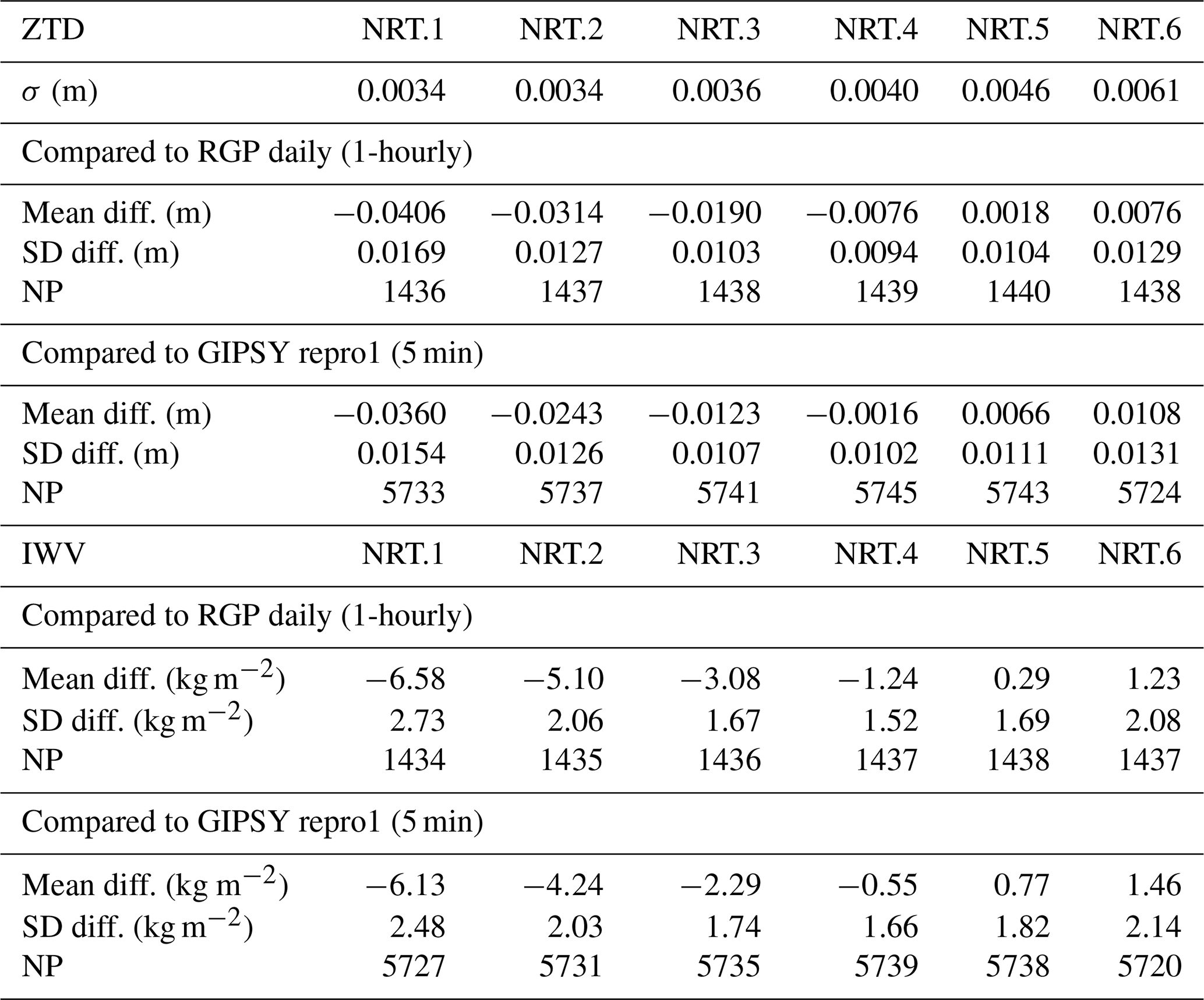
Table 2 RGP NRT ZTD and IWV solutions (NRT.1 to NRT.6) compared to RGP daily and GIPSY repro1, station BCON, period 1 January 2020 to 29 February 2020. In the upper row, “σ” indicates the mean formal error of the RGP NRT solutions (in metres). The comparisons show mean differences (RGP NRT minus RGP daily/GIPSY repro1), standard deviation of differences and the number of points (NP). The RGP daily data sampling is 1 h and the GIPSY repro1 sampling is 5 min.

3 ZTD and IWV intercomparisons at the BCO

In this section, we intercompare both ZTD and IWV results from the five processing streams. The motivation for comparing the ZTD results is that it reflects the uncertainty due to the GNSS processing only, while the IWV comparison includes the conversion errors discussed in the previous section. The uncertainty in the ZTD data is of interest to the data assimilation community since ZTDs are currently assimilated in most NWP models (rather than IWV). On the other hand, the uncertainty in the IWV data may be of interest to users who wish to analyse the IWV directly (e.g. for process studies, intercomparison with other observational techniques, or verification of atmospheric model simulations).

3.1 RGP NRT results

As explained above, in the RGP NRT solution, each hourly time slot is processed six times while it is shifted from the most recent position (referred to as NRT.6) to the oldest (NRT.1) in the 6-hourly time window. The highest precision is expected in the central time slots (NRT.2 to NRT.5) because these are farther from the edges and are best constrained by the observations.

3.1.1 ZTD intercomparison

The overall uncertainty in the NRT solution is mainly due to the ultra-rapid satellite products and small window size (impacting the ambiguity resolution). It can be evaluated by comparison with the RGP daily or any of the GIPSY solutions. The upper part of Table 2 shows the results for the ZTD estimates. The comparison to RGP daily reveals a trend in the mean difference from NRT.1 to NRT.6, with a large negative bias in NRT.1 of −0.04 m (RGP NRT ZTD < RGP daily ZTD). This bias was actually unexpected. It is an artefact due to the propagation of tropospheric gradient biases from one time slot to the next. This feature was corrected in July 2020 and the bias is no longer present in the current operational NRT product. The standard deviation of differences shows a minimum (9.4 mm) for the NRT.4 solution. The values are actually smaller in the central time slots as expected. However, the formal errors (top row of Table 2) predict smaller uncertainty in the first time slot instead. This is a consequence of using the previous normal equations.

The comparison with GIPSY repro1 confirms these conclusions although there are small differences in the results: mainly, the bias is slightly offset by 4 mm. Since this comparison involves two different software and processing approaches, these small differences are not surprising. Note that the number of comparisons is also different by a factor of 4 due to the different ZTD sampling of the three solutions. Compared to GIPSY repro1, the RGP NRT.4 has the smallest bias and standard deviation. We recommend thus to use this solution for near-real-time applications when timeliness is not too restrictive (e.g. in NWP assimilation schemes, the ZTD data from NRT.6 are used, which are a bit less accurate).

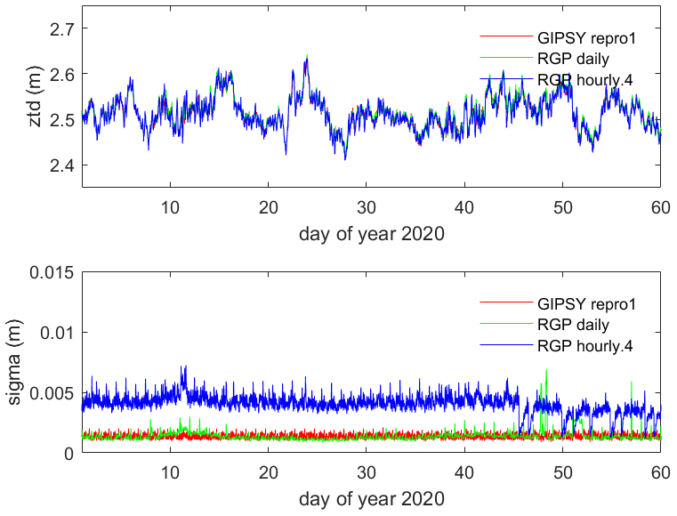
Figure 3 Time series of ZTD estimates and formal errors (σ) from RGP NRT.4, RGP daily, and GIPSY repro1 solutions from 1 January to 29 February 2020.

Figure 3 shows the ZTD and formal error time series from the RGP NRT.4 solution and the other two processing streams. It it seen that the temporal variations in ZTD are very consistent among all three data streams with small differences (<0.01 m) compared to the ZTD variations (0.1 m). On the other hand, the formal errors of the NRT solution are much larger than those of the RGP daily and the GIPSY repro1 solutions. GIPSY repro1 also has more stable formal errors than RGP daily.

3.1.2 IWV intercomparison

The lower part of Table 2 shows the IWV results. In the case of the comparison of RGP NRT to RGP daily, the IWV results are consistent with the ZTD results since both solutions use the same ZHD and K conversion data. The IWV differences are here proportional to the ZTD differences with a factor of 162 kg m⁻³, which is close to the mean value of K=164 kg m⁻³. On the other hand, the comparison with GIPSY repro1 includes the differences in the conversion data, and the ratio of IWV-to-ZTD results is not a constant factor. This point is further discussed in the next subsection. Similar to the ZTD results, the IWV solution for NRT.4 is in good agreement with RGP daily and GIPSY repro1.

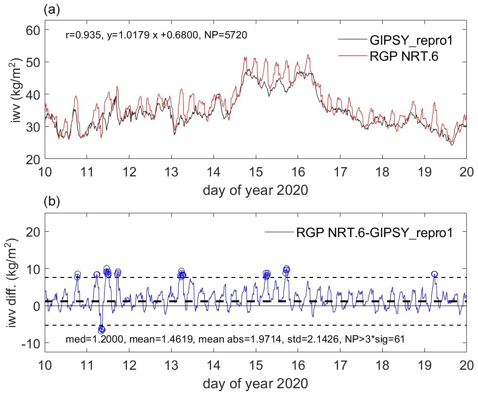
Figure 4 Time series of IWV from near-real-time GNSS processing (RGP NRT.6) compared to post-processed GNSS (GIPSY repro1) from 10 to 20 January 2020. Panel (a) shows the IWV time series and panel (b) the IWV difference (NRT minus repro1).

Figure 4 compares the NRT.6 IWV estimates to GIPSY repro1 for the time period from 10 to 20 January 2020 marked by a period of 2 d with high IWV around 45 kg m⁻². It is striking that the NRT.6 solution shows spurious oscillations with a period about 1 h. This feature is due to the strong relative constraint (1 mm) in the NRT solution with an hourly update. The constraint is the same in the NRT.4 slot but the oscillation is strongly damped (not shown). This result also indicates that the NRT.4 solution rather than the NRT.6 solution should be used when relevant.

3.2 RGP daily and GIPSY results

Similar ZTD and IWV comparisons have been performed for the other processing streams which are of interest for offline applications.

Table 3 Similar to Table 2 but for RGP daily, GIPSY rapid, and GIPSY repro1 results for stations BCON and BCOS. The leftmost part shows ZTD results and the rightmost shows IWV results.

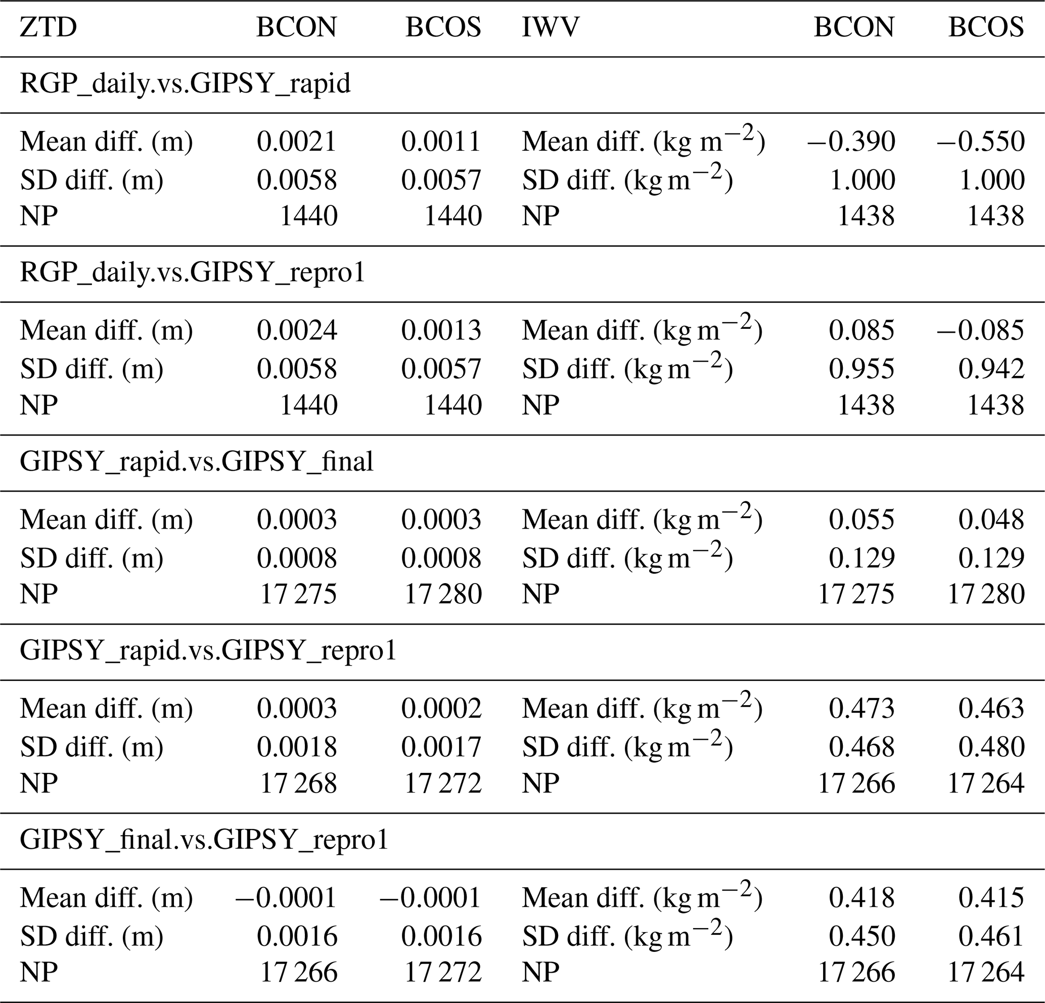
The left part of Table 3 shows the ZTD comparison results. The comparisons of RGP daily to GIPSY rapid and repro1 show very similar results. The agreement between the two processing softwares is quite good, with a small difference in the mean values of 2.1–2.4 mm for station BCON and 1.1–1.3 mm for station BCOS. The standard deviations of ZTD differences are about 5.7–5.8 mm for both stations. The differences reflect mainly the impact of using different satellite products, mapping functions, tropospheric model constraints, and elevation cutoff angles. The comparisons of the three GIPSY solutions show comparatively much better agreement with almost no bias (the mean differences are around −0.1 to 0.3 mm) and very small standard deviations (0.8 to 2.8 mm). The comparison of the two operational solutions (GIPSY rapid and final) shows the smallest standard deviation because they use exactly the same processing options; the only difference is in the satellite products but they were produced by the same analysis centre (JPL) and are highly consistent. The comparison of the GIPSY operational solutions to repro1 shows slightly larger differences which are due to small differences in the processing options.

IWV comparisons have been performed for the same five combinations. In addition to the ZTD differences, due to the processing strategies, these comparisons will include the effect of the IWV conversion methods:

• RGP daily and GIPSY rapid differ by ZHD (PTU vs. TUV) and K (Bevis vs. TUV); strong impact is expected from differences in both parameters;

• RGP daily and GIPSY repro1 differ by ZHD (PTU vs. ERA5) and K (Bevis vs. ERA5); strong impact is expected from K;

• GIPSY rapid and final use the same conversion parameters;

• GIPSY rapid and final differ from repro1 by ZHD and K (TUV vs. ERA5); strong impact is expected from ZHD.

The right part of Table 3 shows the IWV results and confirms they include additional errors compared to the ZTD results (left part the table). Most notably, (i) a change in the bias between RGP daily – GIPSY rapid and RGP daily – GIPSY repro1 because the two GIPSY solutions use different parameters. In the first comparison, the bias is due to the ZHD data used in the GIPSY rapid solution (TUV) and the K data in the RGP daily solution (due to the Bevis et al., 1994 formula). In the second comparison, only the K bias in the RGP rapid solution is involved. (ii) A noticeable bias and standard deviation between the two operational GIPSY solutions and the repro1 due to the ZHD data used in the former (TUV). The two operational GIPSY solutions are highly consistent in IWV (similar to the ZTD solutions) but this result hides the fact that they include common ZHD errors.

Table 4 Separation of bias (mean) and random errors (1 standard deviation) of IWV differences into contributions from ZTD differences, ZHD differences, and K differences, for two operational data streams (RGP daily and GIPSY rapid) and the reprocessed stream (GIPSY repro1). The three streams involve different auxiliary data for the ZTD-to-IWV conversion from PTU, TUV, and ERA5. See text for more details.

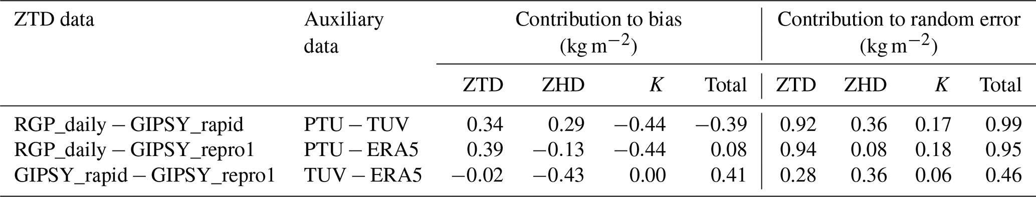
Table 4 quantifies more precisely the contributions from the difference error sources (ZTD, ZHD, and K) to the total IWV differences, where the mean and random components have been separated according to Eqs. (9) and (10). The following can be seen:

• In the RGP daily and GIPSY rapid comparison, all three error sources contribute in the same proportions to the bias, while the random errors are dominated by ZTD errors.

• In the RGP daily and GIPSY repro1 comparison, the small bias in RGP daily is a result of almost exact cancelling of a ZTD bias and a K bias in the RGP data. The random errors in the RGP data are again dominated by ZTD errors.

• In the GIPSY final and repro1 comparison, the bias in the GIPSY final is almost only due to a bias in ZHD, while the random errors are due to ZTD and ZHD differences of the same magnitude.

In conclusion, compared to the GIPSY repro1 data set which uses the most accurate data processing and conversion parameters, both operational streams show small systematic and random errors on the level of ±0.5 and ±1.0 kg m⁻², respectively.

3.3 GNSS compared to other IWV data sources

Two other instruments operated at the BCO facility are used here: the Vaisala RS41/MW41 radiosonde system (Stephan et al., 2021) and the Radiometer Physics GmbH (RPG) HATPRO-G5 microwave radiometer (MWR) (Rose et al., 2005). The IWV retrievals from these systems were compared to IWV estimates from the BCON GNSS station (GIPSY repro1) and ERA5 IWV data for the period from 1 January to 29 February 2020. For the radiosondes, the level-1 pressure (P), temperature (T), and relative humidity (RH) data were used and IWV was computed as

$$\begin{array}{}\text{(11)}& {\mathrm{IWV}}_{\mathrm{RS}}=\underset{P_{\mathrm{GPS}}}{\overset{P_{\mathrm{top}}}{\int }}q\left(P\right)/g\left(P\right)\mathrm{d}P,\end{array}$$

where the integral extends from the GNSS station height to the top of the sounding (24 km on average), q(P) is the specific humidity computed from RH and T using Tetens (1930) saturation pressure formula over water, and g(P) is the acceleration of gravity as a function of altitude. The 1 s time sampling of the radiosonde data provides high vertical resolution (about 5 m in the lower troposphere). They were checked for consistency and thinned for including only increasing altitude points. Very few data gaps were noticed in the vertical profiles, which confirms that the sounding operations worked fine all along the campaign and did not need further correction or screening. The BCO soundings provided a nearly continuous sampling of the upper air conditions between 16 January and 19 February, every 4 h (Stephan et al., 2021). The MWR worked for a more extended period from 1 January to 15 February. The brightness temperature measurements were used to retrieve IWV using a neural network algorithm provided by the manufacturer. In precipitating conditions, the measurements usually experience strong biases due to wet radome emissions (see Fig. 5) and are screened out according to a rain detection index (including also sea spray detection). The IWV contents are nominally retrieved with a 1 s sampling, which we downscaled to 5 min, by computing arithmetic means to be consistent with the GNSS sampling. Some outliers remained in the MWR IWV series which were subsequently removed from the comparisons by a simple outlier check of the IWV differences with limits of mean ±3 standard deviations.

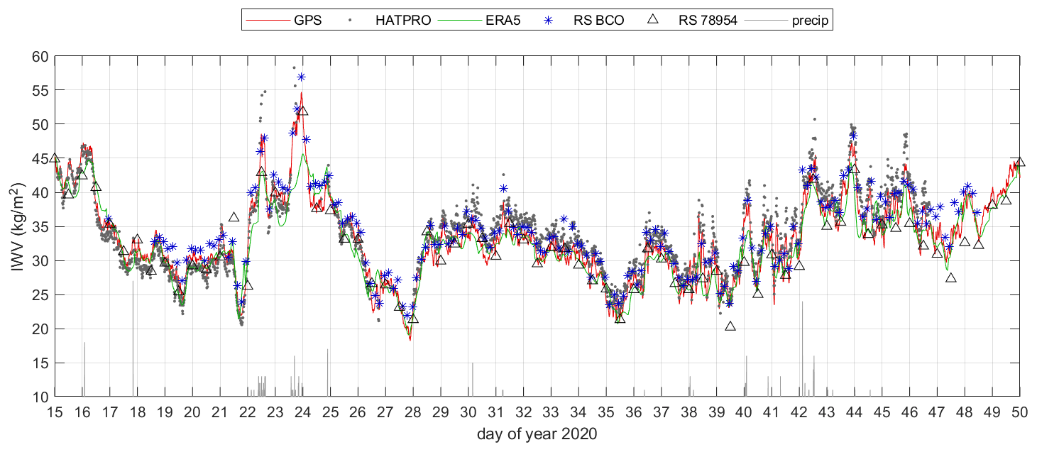
Figure 5 Time series of IWV from GNSS station BCON, RS41 sondes, and HATPRO microwave radiometer collocated at BCO, as well as operational sondes from Grantley Adams International Airport (WMO ID 78954) and ERA5 reanalysis, from 15 January to 19 February 2020. The vertical grey bars at the bottom of the plot show precipitation data collected at BCO.

The ERA5 IWV contents above the GNSS station were computed from the hourly pressure-level data at the four surrounding grid points and interpolated bilinearly to the position of the GNSS antenna. The use of pressure-level data instead of model-level data induces a minor bias of 0.2±0.1 kg m⁻² but these data are more convenient to use and consistent with the T_m computation (see Sect. 2.3.3).

In addition, we also included the twice-daily (00:00 and 12:00 UTC) radiosonde measurements from the operational radiosonde station at Grantley Adams International Airport (GAIA, WMO code 78954) located 11 km away from the BCO. This station used GRAW DFM-09 at the time of the campaign (Kathy-Ann Caesar, personal communication, 2021). The sonde data were retrieved from the University of Wyoming sounding archive and contained on average 85±6 vertical levels up to an altitude of 29±2 km. The vertical sampling of these data is coarser than the BCO data but fine enough to compute proper IWV contents. The latter were computed in a similar way to that for the BCO soundings except near the surface where the ERA5 pressure-level data were used to complete the sounding profiles. This is because the GAIA station is located at an altitude of 57 m, slightly above the BCO, which is at 25 m altitude.

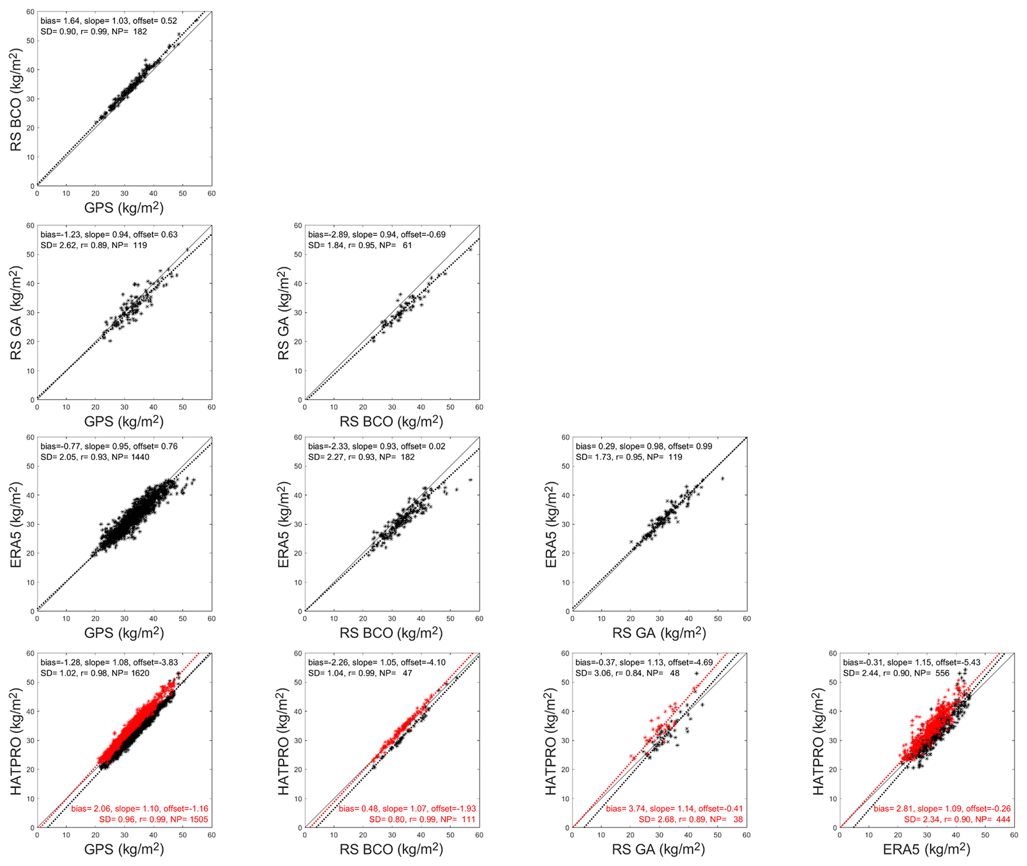
Figure 6 Pairwise scatter diagrams of IWV estimates from GNSS station BCON (GPS), HATPRO MWR, Vaisala RS41 radiosondes released from the BCO (RS BCO), operational radiosondes released from Grantley Adams International Airport (RS GA), and ERA5 reanalysis. The HATPRO data set has been separated in two parts: before (black symbols) and after (red) 27 January when the system was fixed for an instrumental failure. Note that sample sizes are different between diagrams because each comparison is done with the highest temporal resolution for the period of available data between 1 January and 29 February 2020.

Figure 5 shows the IWV time series of the different data sources at their nominal time resolutions. The period underwent large moisture variations with IWV fluctuations between 20 and 55 kg m⁻². Several remarkable situations are observed, such as the peaks on 22 January around 12:00 UTC and 24 January around 00:00 UTC and a few more in February (days 40, 42, 43–44, 45). The agreement between the five data sets is good in general but ERA5 is seen to underestimate the IWV during the aforementioned peaks. Quite obvious is also the bias between the two sounding data, with the BCO IWV contents systematically higher than the GAIA measurements. Less easy to distinguish, but nevertheless significant, is the offset in the HATPRO MWR IWV retrievals before and after 27 January. The HATPRO data are actually more consistent with the GAIA data before that date and instead more consistent with the BCO radiosonde data after. Analysis of the measured brightness temperatures showed that during the former period, the measurements were less accurate due to an instrumental malfunction which was fixed on 27 January.

Figure 6 compares the IWV data from the five sources pairwise and includes some consistency statistics. The slope and offset parameters were fitted using the York et al. (2004) method to account for errors in both coordinates. For both radiosondes and HATPRO, the uncertainty in the IWV estimates was assumed to be 5 %. For ERA5, the uncertainty was computed as the max − min of the IWV values at the four surrounding grid points before the horizontal interpolation, which is a measure of the representativeness error (Bock and Parracho, 2019). The uncertainty estimates over the study period were $\mathrm{1.71}\pm \mathrm{0.31}\mathrm{kg}{\mathrm{m}}^{-\mathrm{2}}$ for the BCO soundings, $\mathrm{1.57}\pm \mathrm{0.28}\mathrm{kg}{\mathrm{m}}^{-\mathrm{2}}$ for the GAIA soundings, $\mathrm{1.65}\pm \mathrm{0.25}\mathrm{kg}{\mathrm{m}}^{-\mathrm{2}}$ for HATPRO, and $\mathrm{1.48}\pm \mathrm{0.86}\mathrm{kg}{\mathrm{m}}^{-\mathrm{2}}$ for ERA5. For GNSS, the ZTD formal errors were converted to IWV and rescaled with a factor of 5 in order to be consistent with the other data sources, yielding a final GNSS IWV uncertainty of $\mathrm{1.15}\pm \mathrm{0.16}\mathrm{kg}{\mathrm{m}}^{-\mathrm{2}}$.

Results from the GPS, the BCO and GAIA sondes, and the ERA5 comparisons are reported in Fig. 6. While IWV varies from 20 to 55 kg m⁻² over the period, the bias between the two sondes is −2.89 kg m⁻² (GAIA – BCO) with a slope of 0.94 and an offset of −0.69 kg m⁻². The GAIA data are drier than the BCO data over the full observation range. The comparison of profiles shows that the humidity measurements from the two sondes differ mainly in the lowermost 2.5 km where the mean difference in q is larger than 1 g kg⁻¹. One contribution to this difference may be the difference of trajectories of the sounding balloons released from the two sites. Balloons released from the BCO site usually travel west and southwards over the island of Barbados until they reach an altitude of 6–8 km when they enter the westerly jet. The balloons released from GAIA drift in similar directions but arrive earlier over the open sea as they are released from the southern part of the island. A small “island effect” might show up here as the moisture profiles over the island of Barbados seemed to be slightly moister than those over the nearby sea during the EUREC⁴A field campaign (Fig. A4 in Stephan et al., 2021). Another contribution might arise from moisture transport associated with land and sea breezes as was previously evidenced in Colombo, Sri Lanka, where the land–sea breezes contributed to a daytime boundary layer moistening and nighttime drying observed in radiosoundings (Ciesielski et al., 2014a). The moisture observations at the BCO exhibit actually a day–night variation in IWV of 1.7 kg m⁻², whereas the variation at GAIA is significantly smaller (1.1 kg m⁻²). Although both effects are not negligible, they are not large enough to explain the mean bias between the BCO and GAIA sondes. Instead, we suspect the difference in sonde types to play a more central role.

The Vaisala RS41 sondes used at BCO are from the last generation of sondes and are considered to provide significantly improved temperature and humidity measurements compared to previous sonde types (e.g. Vaisala RS92) especially in cloudy conditions (Jensen et al., 2016). High confidence in the BCO soundings suggests that the GAIA soundings have a significant dry bias which may impact humidity analyses from NWP models that assimilate these observations. This seems to be the case for ERA5 and would explain the high consistency between ERA5 and GAIA IWV estimates (bias of 0.29 kg m⁻² and near-unity slope) and the large difference of ERA5 compared to the BCO (bias of −2.33 kg m⁻² and slope of 0.93). The GNSS IWV estimates are intermediate between the two sounding results. Using GNSS as the reference, we conclude that there is a wet bias in the BCO radiosonde data of 1.64 kg m⁻² and a dry bias in the GAIA radiosonde data (−1.23 kg m⁻²) as well as in the ERA5 data (−0.77 kg m⁻²). On the other hand, using the BCO sounding data as a reference, one would conclude on a dry bias in all other IWV estimates, except the HATPRO MWR after the instrumental fix on 27 January, where the MWR retrieval is slightly moist. Since no reference water vapour measurements were made at the same time, it is difficult to establish the absolute sign of these biases. The GNSS − RS41 bias of −1.64 kg m⁻² observed here represents a fractional bias of 5 % which is slightly larger the uncertainty of both systems and thus needs to be explained. From our previous experience comparing Vaisala RS92 sondes and GNSS IWV estimates (produced using the same approach as in this study), we observed slightly smaller biases of ±0.5 to 2 % (Bock et al., 2016). Further investigation is needed in the case of the RS41 vs. GNSS comparisons.

The comparison of HATPRO IWV retrievals has been separated into two batches (before and after 27 January). Compared to GNSS, the bias before (after) is −1.28 (+2.06) kg m⁻² with a slope significantly larger than 1 indicating that the bias increases with the amount of IWV. Similar slope values are obtained in the comparison to the other data sources, which might be attributed to the MWR training data set (Rose et al., 2005). Occurring biases could be further corrected by applying a clear-sky brightness temperature offset correction based on sounding data. In terms of temporal variability, the MWR, GNSS, and BCO sondes are in good agreement (standard deviation of differences ∼1 kg m⁻² and correlation coefficient ≥0.98). The bias with respect to the BCO soundings is 0.48 kg m⁻² (MWR too moist) during the second period, but this bias is within the known uncertainties.

Figure 7 Humidity profiles from BCO and Grantley Adams radiosondes (WMO ID 78954) on (a, b) 22 January 2020 at 12:00 UTC and (c, d) 24 January 2020 at 00:00 UTC (exact times are indicated in the plot legend).

ERA5 is biased low compared to both GNSS and BCO sondes with slopes lower than 1, meaning that the dry bias increases at larger IWV values. The scatter plots in Fig. 6 exhibit a few outlying values which correspond to the situation when ERA5 underestimates the IWV peaks during the period 22–24 January (see Fig. 5). Quite surprisingly, the GAIA soundings during this period, although slightly drier, are much closer to GPS and BCO than ERA5. Inspection of the vertical humidity profiles (Fig. 7) shows that ERA5 is close to the GAIA observations in the lower 2–2.5 km but does not account for the vertical extension and the sharp drop in humidity at the top of the deep moist layer around 3–4 km on 22 January and around 5 km on 24 January. The misrepresentation of the relative humidity profile is spectacular on 24 January at 00:00 UTC. This might be due to the assimilation of other data (e.g. satellite humidity sounders) that are biased low in the mid-troposphere during this event. Inspection of radar reflectivity measurements from the BCO reveals that on both dates heavy rain was occurring over an extended part of the lower troposphere (up to 3.5 km height on 22 January around 10:00–11:00 UTC and 5.0 km on 23 January around 22:00–23:00 UTC). This would explain the saturated air (RH =100 %) below 3 km for the former and below 5 km for the latter of the two BCO soundings. The GAIA soundings mimic the BCO soundings but with a dry bias within these rainy layers. Above this layer, it seems that the GAIA sondes have a moist bias, probably due to rain contamination of the humidity sensor, a problem that is corrected in the design of the newer RS41 sondes (Jensen et al., 2016). Above the moist layers, ERA5 fits well the BCO profiles.

Table 5 Pairwise comparison of IWV estimates from GNSS station BCON (GPS), HATPRO MWR, Vaisala RS41 radiosondes released from the BCO (RS BCO), operational radiosondes released from Grantley Adams International Airport (RS GA), and ERA5 reanalysis. The HATPRO data set has been separated in two parts: before and after 27 January when the system was fixed for an instrumental failure. For each period, the data from all sources have been time matched.

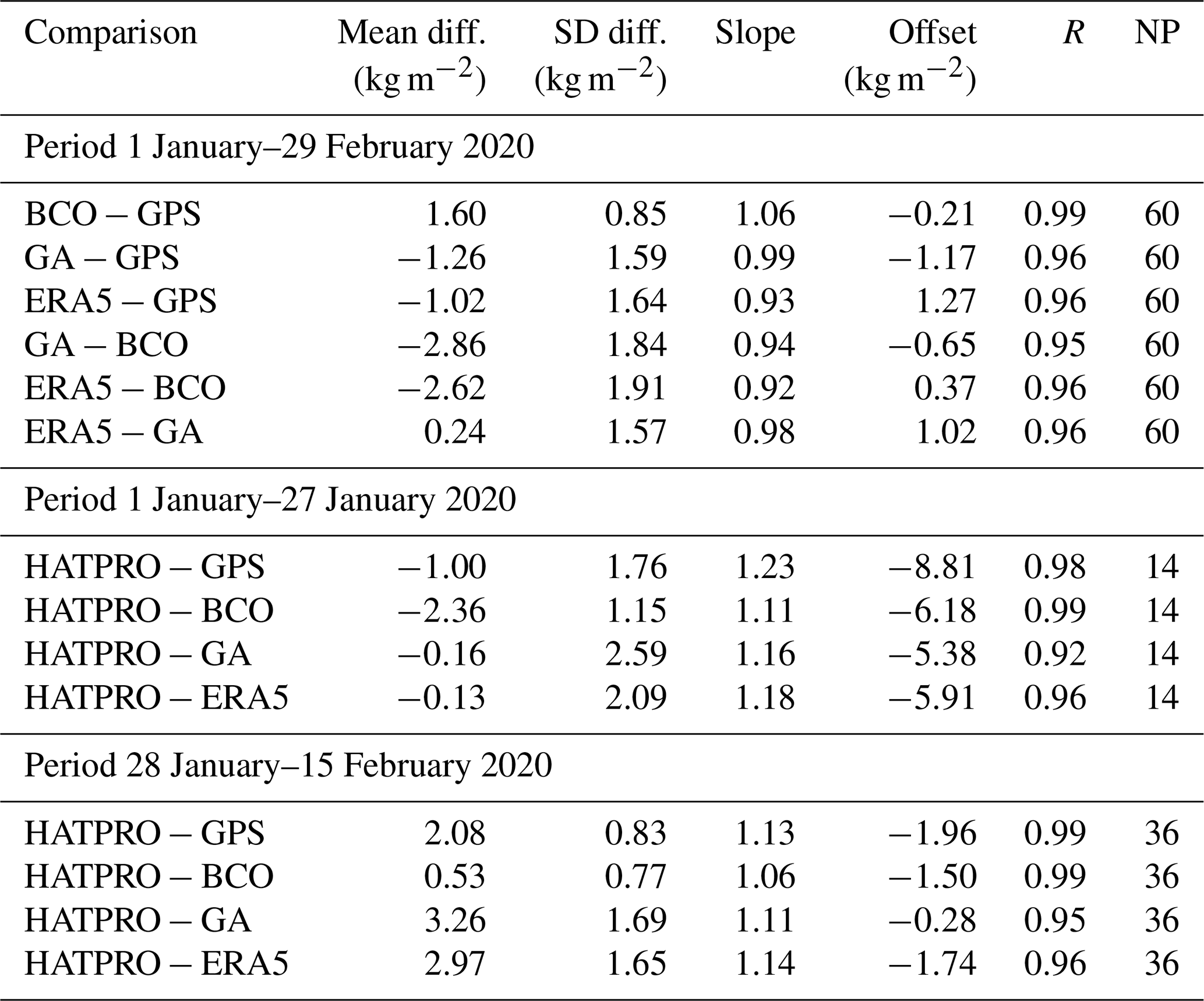
Complementary statistics are reported in Table 5, where the data have been time matched. The conclusions are essentially the same as discussed above, but the pairwise biases can be more easily compared and combined.

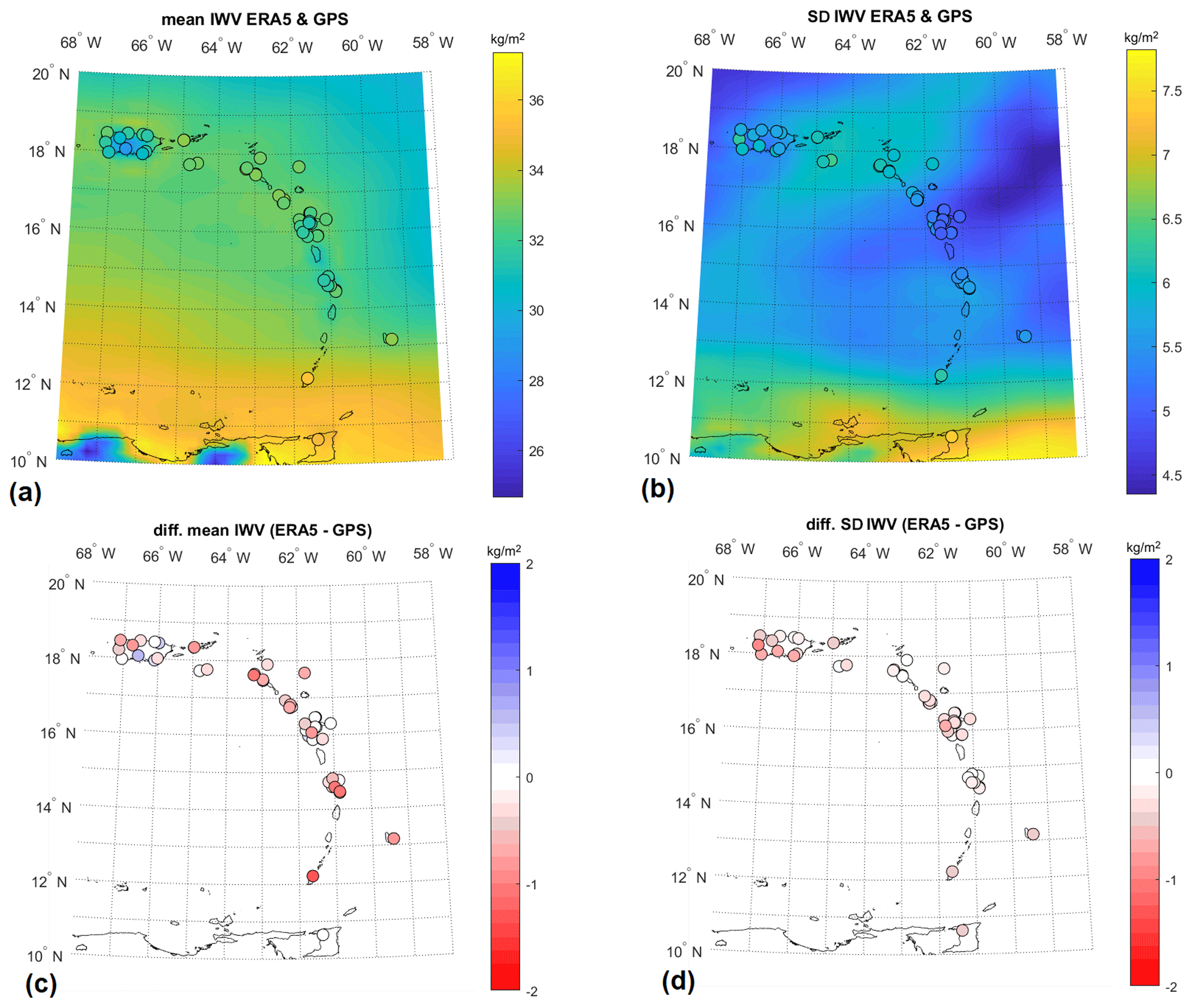
Figure 8 (a, b) Mean and standard deviation of hourly IWV from ERA5 (background) and GNSS (circles) from 1 January to 29 February 2020. (c, d) Difference of mean and standard deviation of hourly IWV values (ERA5 − GNSS). In panels (a) and (b), the GNSS IWV data have been height corrected and gaps have been filled with ERA5 values to minimize representativeness differences. In panels (c) and (d), ERA5 IWV data have computed from pressure-level profiles from the height of the GNSS stations upwards (no correction applied to GNSS IWV data).

4 Spatiotemporal distribution of IWV at the regional scale

4.1 Comparison of IWV retrievals from GNSS network and ERA5 reanalysis

Figure 8 shows the mean and standard deviation of hourly IWV from ERA5 and GNSS for the 2-month period. The mean IWV is seen to be relatively uniform over the region, with a small SW–NE gradient correlated with the sea surface temperature (SST) gradient (SST decreasing towards the NE). The maximum, around 35 kg m⁻², is observed below 13^∘ N in the more tropical part of the domain, and the minimum to the NE is around 30 kg m⁻². The mean ERA5 field is generally in good agreement with the GNSS observations over the Caribbean arc (CA), with an exception over Puerto Rico (18^∘ N, 67^∘ W), where ERA5 has a small dry bias (0.5–1 kg m⁻²). On average, over all stations, the mean difference (ERA5 − GNSS) is $-\mathrm{0.34}\pm \mathrm{0.50}$ kg m⁻², pointing to a small dry bias of ERA5 in the region with some site-to-site variation. This result is consistent with the bias that is discussed in the previous section based on BCO results, and also with the results of a previous study (Bosser and Bock, 2021). But further investigation is needed to explain the reason for this dry bias in ERA5 (e.g. its link with the data assimilation). In terms of temporal variability, the agreement between ERA5 and GNSS is also quite good, except over Puerto Rico. There is significant spatial modulation of the magnitude of variability. Again the maximum is observed to the south over the tropical Atlantic Ocean. The average difference of standard deviation (ERA5 − GNSS) is −0.25 kg m⁻², meaning that the variability in ERA5 is slightly underestimated compared to GNSS. This may be partly due to a difference in representativeness between the GNSS point observations and the gridded reanalysis fields (Bock and Parracho, 2019) and partly to some special situations where the reanalysis underestimates high-IWV contents (see Fig. 5).

Table S2 in the Supplement gives the comparison results for all stations. The mean and standard deviation of IWV differences (ERA5 − GNSS) have been cross-compared with the GNSS data quality diagnostics from Table S1 and no significant correlation was found. We therefore believe the main differences are not due to GNSS uncertainties but rather to differences in representativeness such as evidenced particularly over Puerto Rico. Closer inspection of the ERA5 orography for this island shows that the topography is largely misrepresented in the model where the highest elevation is 316 m above sea level, whereas the real topography reaches 1338 m. Also, the latitudinal extension of the island is exaggerated (e.g. GNSS station EMPR at 18.47^∘ N is at an altitude, or geoid height, of 10 m, whereas the nearest model grid point at 18.5^∘ N is at an altitude of 103 m). Since almost all the stations considered in this study are located on small volcanic islands with steep topography, the misrepresentation of the topography is a major source of uncertainty in the GNSS and ERA5 comparison. This poses also some problems to the assimilation of observations taken from surface meteorological stations and upper air soundings.

4.2 Couplings between clouds, circulation, and humidity at the synoptic scale

To illustrate the spatiotemporal variability of IWV at the regional scale, we have selected five GNSS stations representative of the different parts of the Caribbean arc (CA). The GNSS station CRO1 (St. Croix, US Virgin Islands; 17.76^∘ N, 64.58^∘ W) was chosen as being representative of the northern CA. The GNSS station of LDIS (Guadeloupe; 16.30^∘ N, 61.07^∘ W) and FFT2 (Martinique; 14.60^∘ N, 61.06^∘ W) were chosen as being representative of the central CA, GNSS station BCOS (13.16^∘ N, 59.42^∘ W) was selected as being representative of Barbados, and the GNSS station of GRE1 (Grenada; 12.22^∘ N, 61.64^∘ W) was selected for the southern CA. The selection accounted for the continuity of the series (ideally 1440 hourly IWVs over the 2 months of January and February 2020) and the processing quality diagnostics (see Sect. 2.3.3 and Table S1). For the islands associated with several stations (e.g. 15 for Guadeloupe and 6 for Martinique), the GNSS station with the most complete IWV series and the best data quality was chosen.

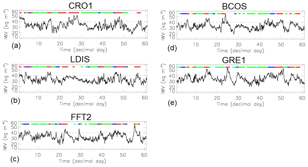
Figure 9 Time series of IWV from five GNSS stations for the period from 1 January to 29 February 2020 as well as the type of cloud patterns in the vicinity of the GNSS sites (see colour code in Fig. 11).

The IWV times series associated with the five GNSS stations are shown in Fig. 9. They highlight substantial variability in the course of the January–February 2020 period, alternating moist (in excess of 50 kg m⁻²) and dry (below 20 kg m⁻²) episodes, sometimes within a few days as, for instance, in Barbados where GNSS-derived IWV was observed to decrease from 54.3 to 17.8 kg m⁻² between 23:00 UTC on 23 January and 21:00 UTC on 27 January 2020 (Fig. 9d). Unsurprisingly, the time series of the five GNSS stations spanning over a region of 6^∘ in latitude do not show obvious correlations, suggesting that they are not influenced by the same IWV-impacting weather at the same time in the course of the 2 months.

Among the processes likely to strongly impact the IWV fields in the trade winds, shallow convection is of paramount importance. Stevens et al. (2020) have shown that cloud mesoscale organization in the trade winds is dominated by four main patterns referred to as Fish, Flowers, Gravel, and Sugar. These patterns have also been shown to depend on environmental conditions (Bony et al., 2020; Rasp et al., 2020; Schulz et al., 2021). The clouds embedded in these patterns are characterized by different vertical and horizontal extensions, reflectivity, separation, etc. For instance, it has been shown that the clouds compositing Fish, Gravel, and Flowers patterns have similar vertical extent (see Stevens et al., 2020, their Fig. 9, based on radar observations in Barbados) but are different from the small clouds composing the Sugar pattern. For details on the characteristics of the four cloud patterns, the reader is referred to Stevens et al. (2020) and Schulz et al. (2021).

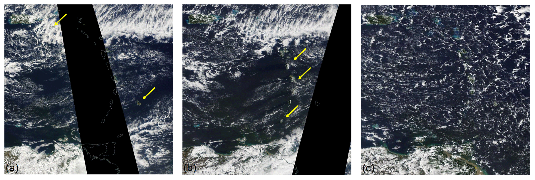
Figure 10 Visible image from (a) MODIS Aqua and (b) Terra, on 19 January 2020, and (c) MODIS Aqua, on 13 January 2020, depicting different cloud organization over the study domain (8.9–19.1^∘ N, 57.4–67.6^∘ W). The yellow arrows locate St. Croix (northwest) and Barbados (southeast) in the upper left image, and Guadeloupe, Martinique, and Grenada (from north to south) in the upper right image. In the lower image, a Gravel cloud organization is observed uniformly across the domain on 13 January 2020. Source: NASA WorldView (https://worldview.earthdata.nasa.gov/, last access: 29 January 2021).

In order to obtain a first assessment of the IWV values characterizing the environment of the mesoscale cloud organization in the region of the CA, we have performed a visual classification of the cloud scenes over 60 d (between 1 January and 29 February 2020) over a domain spanning from 57.4 to 67.6^∘ W and from 8.9 to 19.1^∘ N. Our domain is similar in size to the one used by Stevens et al. (2020) for the same months between 2007 and 2016 but shifted west by 10^∘ and slightly south as well to include the CA. The classification was performed by visual inspection of the MODIS Aqua and Terra visible images at 13:30 and 10:30 local Equator crossing time available from NASA WorldView (https://worldview.earthdata.nasa.gov/, last access: 29 January 2021). Unlike Stevens et al. (2020), we did not classify the dominant cloud scenes across the domain but came up with a classification of the cloud scenes around each of the selected GNSS stations in order to more accurately link GNSS-derived IWVs with cloud organization. This was necessary as on some days the different parts of the domain were not under the influence of the same cloud pattern as, for example, shown in the Aqua and Terra MODIS images on 19 January 2020 (Fig. 10). On that day, St. Croix was under the influence of a Fish pattern, while Barbados was surrounded by clear air. The clear-sky band in between two cloud clusters is actually part of the Fish pattern. Guadeloupe was located off the southern edge of the Fish structure and was surrounded by Gravel, while Martinique and Grenada further south were bordered by Sugar. On other days, such as 13 January 2020, Gravel was observed to be uniformly spread across the CA domain (Fig. 10). The classifications performed for each of the five sites in January and February 2020 are provided in Fig. 11.

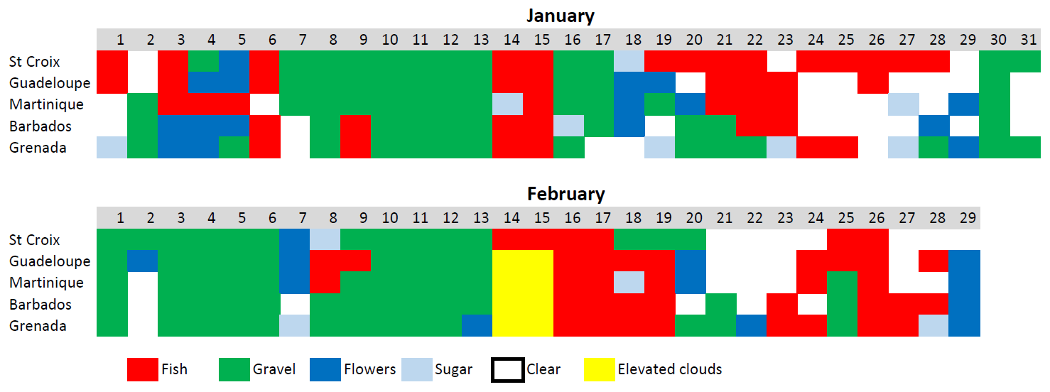
Figure 11 Cloud type classification performed for each of the five sites in January and February 2020.

Table 6 Upper part: number of cases over the five sites of interest in the Caribbean arc in January and February 2020 for each cloud organization type (Fish, Flower, Gravel, Sugar, or lack thereof) according to the classification of (Stevens et al., 2020). The cases were identified by visual inspection of the MODIS Aqua and Terra visible images at 13:30 and 10:30 local Equator crossing time available from NASA WorldView (https://worldview.earthdata.nasa.gov/, last access: 29 January 2021). Lower part: mean and standard deviation of GNSS-derived IWVs associated with Fish, Gravel, Flowers, and clear conditions.

For each of the five GNSS stations representative of the different parts of the CA, the time series of cloud classification is also shown, with Fish appearing in red, Gravel in green, Sugar in light blue, Flowers in dark blue, and cloud-free conditions in white. As also observed by Stevens et al. (2020) between 2007 and 2016, the Gravel type was the dominant mode of cloud organization over the CA during January and February 2020, with a number of cases ranging from 19 in Guadeloupe to 27 in Grenada (Table 6). Fish was the next most dominant pattern of cloud organization, with a number of cases ranging from 10 in Martinique to 19 in St. Croix and Guadeloupe. Sugar was the least observed cloud pattern (between 0 and 6 cases depending on the site), as also demonstrated by Stevens et al. (2020). Flowers were observed more often in the central and southern part of the CA (between 8 to 11 d) than in the northern part (on 3 d only). Finally, cloud-free cases in between Fish and Flowers were also observed on more than 10 d during the period of interest, except in the southern part of the CA where only a few cloud-free days are observed.

Table 7 Significance of differences in the means of IWV samples using a Student's t test across all stations. “Yes” means that the means are statistically different at the 0.05 level.

From the time series of IWV and the cloud classification shown in Fig. 9, and if we consider the two most dominant modes, the picture emerges that the Fish pattern (in red) is more systematically associated with higher IWV values than the Gravel pattern (in green). This visual impression is confirmed when computing the average IWV values associated with Fish and Gravel patterns over the five stations (Table 6). The mean IWV values in the Fish environment are found between 40.5 and 35.1 kg m⁻², while their counterparts in the Gravel environment range between 33.1 and 30.8 kg m⁻². Differences in the mean Fish-related and Gravel-related IWV values range between 4.3 kg m⁻² (Guadeloupe) and 7.4 kg m⁻² (Grenada), and are found to be significant using a Student's t test (see Table 7). Clear scenes over the islands of interest are also seen to be associated with rather dry conditions, whereas Flowers are associated with intermediate moister conditions with mean IWV values ranging between those of Fish and Gravel. The differences in the mean Fish-related and clear-condition IWV values are also found to be significantly different (the difference ranging between 8.4 kg m⁻² in St. Croix and 5 kg m⁻² in Guadeloupe). Student's t tests also reveal that the difference in the IWV means of all the other pairs (i.e. Fish–Flowers, Gravel–Flowers, Gravel–Clear conditions, and Flowers–Clear conditions) are not significant.

From our analysis, it also appears that ambient conditions in Grenada are moister than in the rest of the CA (this is reflected in both the Fish-related and the Gravel-related mean IWV values), which is likely connected to the proximity of the Intertropical Converge Zone located over the northeastern part of South America in boreal winter. Interestingly, the driest conditions are observed in Guadeloupe (the northern part of central CA), which may be an indication of a more pronounced influence of the midlatitudes.

In summary, based on a compilation of IWV values gathered from representative GNSS stations across the CA, we found that the environment of Fish cloud patterns to be moister than that of Flowers cloud patterns which, in turn, is moister than the environment of Gravel cloud patterns. This is consistent with the relative humidity profiles composited by Schulz et al. (2021). Since Fish patterns are associated with weak winds (relative to Flowers or Gravel; Bony et al., 2020), it means that this high humidity is related to mass convergence within the column, associated with ascent. The differences in the IWV means between Fish and Gravel were assessed to be significant. Finally, the Gravel moisture environment was found to be similar to that of clear, cloud-free conditions. The moister environment associated with the Sugar cloud pattern has not been assessed because it was never prominent around the GNSS stations during the first 2 months of 2020 (but Sugar-like clouds occur very often within mesoscale cloud patterns).

In the following, we focus on the specific period during which a large variation of IWV was observed at the GNSS station BCOS in Barbados from 54.3 to 17.8 kg m⁻² between 23:00 UTC on 23 January and 21:00 UTC on 27 January 2020, associated with a transition from a Fish cloud pattern to clear, cloud-free conditions (see the cloud scene classification in Fig. 9d). For the period from 20 to 30 January, the extreme IWV values were indeed observed in Barbados (i.e. values given above), with the closest lowest values being observed in Martinique on 20 January and the closest highest value in St. Croix on 24 January 2020.

On 22 January, a large southeast–northwest-oriented Fish feature was observed with MODIS to extend over a large portion of the CA, from Barbados to Guadeloupe, also covering Martinique (Fig. 13a), while Grenada was located in clearer air south of the Fish, and St. Croix was covered by another distinct Fish feature further north. Figure 14a shows the ERA5-derived IWV field over the same domain as the MODIS Aqua visible image at roughly the same time (∼15:00 UTC) together with the GNSS-derived IWV values (overlain within open white circles at the location of the 49 GNSS stations). The Fish feature extending over the central CA is associated with a plume of rather high IWV over Barbados and Martinique in the ERA5 field but does not reach Guadeloupe, whereas GNSS retrievals indicate higher IWV values in the southern part of the island. The GNSS stations in Barbados, Martinique, and Guadeloupe all show IWV values in excess of 35 kg m⁻² after 12:00 UTC on that day, while lower values are observed in Grenada to the south and St. Croix to the north (Fig. 12). In Barbados, a maximum IWV value of 48.6 kg m⁻² was observed at 12:00 UTC, which is associated with a deep moist lower troposphere as observed from the radiosounding measurements made from the BCO (Fig. 7a and b). Using trajectory analyses from the LAGRANTO Lagrangian analysis tool (Sprenger and Wernli, 2015), Villiger et al. (2020) also evidenced that air parcels arriving at 1000–700 hPa above the BCO are transported from high latitudes towards the BCO by an extratropical surface cyclone/upper-level trough located off the US east coast. The initially dry air parcels descend from upper levels into the boundary layer, where they experience a rapid moistening, before arriving at the BCO as anomalously humid.

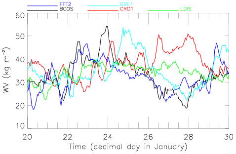
Figure 12 IWV time series observed from GNSS over each of the five sites between 20 and 30 January 2020.

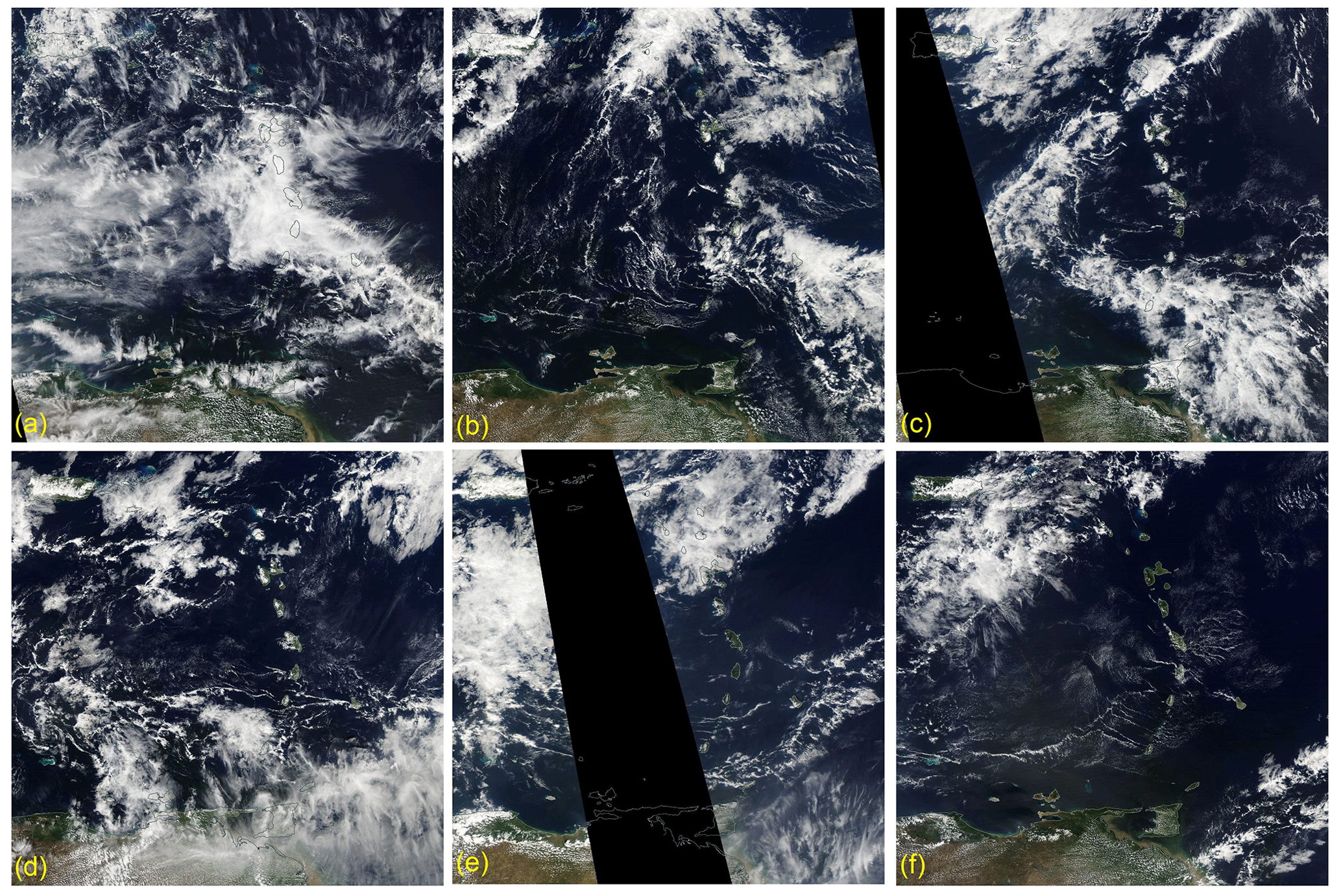
Figure 13 Visible images from MODIS Aqua around 13:30 UTC on each day between 22 and 27 January 2020 (from left to right and top to bottom). Source: NASA WorldView (https://worldview.earthdata.nasa.gov/, last access: 29 January 2021).

Figure 14 IWV fields from ERA5 reanalysis (background) and GNSS (circles) at 15:00 UTC on each day between 22 and 27 January 2020 (see text insert in each image).

On 23 January, a southeast–northwest-oriented Fish feature was also observed with MODIS to extend between Barbados and Martinique. Guadeloupe was under the influence of another distinct Fish feature further north, while Sugar was observed to surround Grenada, and cloud-free conditions were found over St. Croix (Fig. 13b). Three distinct IWV plumes are seen in the ERA5 field: one over Puerto Rico, one further east over the Netherlands Antilles almost reaching Guadeloupe, and one extending from the southeast over Barbados and Martinique (Fig. 14b). Drier air masses are seen in St. Croix (located between two IWV plumes to the north) and in Grenada along the southern edge of the southernmost plume. Comparison between ERA5 and GNSS IWV values suggests that the southernmost plume in ERA5 is located a bit too far south as ERA5 IWVs are underestimated in Barbados and Martinique, and slightly overestimated in Grenada. On that day also, the GNSS stations in Barbados, Martinique, and Guadeloupe all showed IWV values in excess of 35 kg m⁻² after 12:00 UTC, while lower values were observed in Grenada to the south and St. Croix to the north (Fig. 12). The maximum IWV value of 54.3 kg m⁻² observed at the end of the day in Barbados is in good agreement with that derived from the high-resolution radiosounding performed at 22:40 UTC at the BCO (Fig. 5). It exhibits a deep moist layer, with a nearly 100 % relative humidity in the first 5 km of the troposphere (Fig. 7c and d) which was also highlighted by Stephan et al. (2021) (their Fig. 9). Like on 22 January, the moist air below 5 km above the BCO is associated with transport from high latitudes towards the BCO by the extratropical surface cyclone/upper-level trough off the US east coast (Villiger et al., 2020).

On 24 January, the cloud scene over the CA was dominated by Fish features again, with the previously observed southern southeast–northwest-oriented Fish pattern being shifted to the west, clearing most of the central CA and Barbados, while moving over Grenada (Fig. 13c). It merged over the Caribbean Sea with a southwest–northeast-oriented Fish structure going across the CA north of Guadeloupe. St. Croix was underneath a distinct Fish at that time. As a result, Guadeloupe, Martinique, and Barbados were in a mostly cloud-free air mass moving in westward behind the “<”-shaped Fish structure. As shown in Fig. 14c, the “<”-shaped structure of the Fish pattern also reflects in the ERA5-related IWV field, with higher IWV values located to the south of Barbados and to the east of Grenada. The northern branch of the “<”-shaped plume appears to be located too far east in ERA5, as suggested by the slight overestimation of IWVs over Guadeloupe compared to the GNSS retrievals. Consistent with the above-described spatial distribution, the GNSS stations in Grenada show the highest IWV values (reaching 50 kg m⁻²) after 12:00 UTC, while lower similar values (and a similar decreasing trend) are observed in Barbados, Martinique, Guadeloupe, and St. Croix further north (Fig. 12).

On 25 January, Grenada and St. Croix appeared beneath the remains of two distinct Fish features, while cloud-free conditions were observed in the rest of the CA. The central part of the CA was bordered with Sugar to the east (Fig. 13d). The “<”-shaped feature of higher IWVs was still visible in the ERA5 field further west with respect to the previous day, with most of the central part of the CA being located in a drier environment (Fig. 14d). On that day also, the northern branch of the “<”-shaped IWV plume appeared to be located too far east in ERA5. The GNSS stations in Grenada show the highest IWV values after 12:00 UTC even though IWV is observed to decrease on that day as the “<”-shaped plume is moving west. IWV values in Barbados, Martinique, and Guadeloupe are even smaller than the previous days as drier air masses continue to move in from the tropical north Atlantic (Fig. 12). A maximum of IWV is observed in St. Croix in relation to the presence of a Fish feature.

On 26 January, IWV values in Grenada, Barbados, and Martinique continued to drop (Fig. 12) as large-scale cloud features (and related higher IWV values) continue to be advected westward (Figs. 13e and 14e, respectively). Cloud-free conditions now dominated the central part of the domain, while Fish features were observed in the northwestern most corner of the domain, covering both St. Croix and Guadeloupe. As a result, the GNSS station in St. Croix highlighted a maximum of IWV reaching 50 kg m⁻², while larger IWV values than the previous day were also observed in Guadeloupe (Fig. 12), consistent with the spatial distribution of IWV obtained with ERA5 (Fig. 14e).

Finally, on 27 January, a well-defined Fish feature was observed in the north of the domain, covering the US Virgin Islands and St. Croix (Fig. 13f), which was associated with a plume of IWV values between 40 and 50 kg m⁻² (Fig. 14f). All the other stations to the south were located in the drier, mostly cloud-free air mass to the east of the Fish pattern. Martinique and Guadeloupe were surrounded by Sugar, while the environment of Barbados and Guadeloupe was observed to be cloud free (Figs. 11 and 13f). The GNSS station in St. Croix highlighted a IWV maximum of 50 kg m⁻² for the second consecutive day, while in Barbados and Grenada the GNSS stations recorded the lowest IWV values of the period after 12:00 UTC as the driest conditions were evidenced with ERA5 over the tropical North Atlantic east of the central CA (Fig. 14f). In Martinique and Guadeloupe, higher IWV values were observed (between 30 and 35 kg m⁻²) after 12:00 UTC (Fig. 12) as both stations appeared to be located in regions of IWV gradients west of the drier air masses (Fig. 14f).

It is also worth noting that from 16 to 22 January, the IWV features as modelled with ERA5 were moving westward across the CA domain (not shown). On 22 and 23 January, IWV features remained quasi-stationary, while from 24 January onward, there was a clear decoupling between the northern and southern parts of the domain, with IWV features north of 14^∘ N being advected eastward and IWV structures south of 14^∘ N moving westward. This is the origin of the “<”-shaped IWV feature seen on 24 and 25 January (Fig. 14c and d) as well as the “<”-shaped Fish pattern observed in the MODIS images (Fig. 13c and d). The eastward motion north of 14^∘ N on 24 and 25 January is likely related to the growing influence of an extratropical disturbance (sea surface pressure of 1005 hPa, not to be confused with the extratropical cyclone off the US east coast) that formed north of Puerto Rico on 22 January, with its centre located at 30^∘ N, 65^∘ W, and moved northeastward in the following days (the centre of the disturbance was located at 35^∘ N, 45^∘ W, on 25 January).

5 Code availability

GIPSY OASIS II version 6.2 software used to process the GNSS observations is owned by the California Institute of Technology (Caltech). Licensing requests are available from https://gipsy-oasis.jpl.nasa.gov (last access: 26 May 2021) for academia (which are free of license fees), industry, and government.

6 Data availability

This paper used the Vaisala RS41 radiosonde measurements from the EUREC4A field campaign, v2.2.0, available from AERIS: https://doi.org/10.25326/62 (Stephan, 2020).

The GNSS RINEX data used in this work are available from the following data servers:

• RGP: ftp://rgpdata.ign.fr/pub/data/, last access: 29 January 2021;

• UNAVCO: ftp://data-out.unavco.org/pub/rinex/, last access: 29 January 2021;

• ORPHEON: http://reseau-orpheon.fr/, last access: 29 January 2021;

• SONEL: https://www.sonel.org/, last access: 29 January 2021.

The ORPHEON GNSS RINEX data are provided for scientific use in the framework of the GEODATA-INSU-CNRS convention. The DOI references for the UNAVCO GNSS RINEX data are listed in Table A1 in the Appendix.

The GIPSY reprocessed ZTD and IWV estimates from the 49 GNSS stations used in this study are available from AERIS, the French national data and service portal for the atmosphere (https://www.aeris-data.fr/, last access: 29 January 2021), under https://doi.org/10.25326/79 (Bock, 2020b).

7 Discussion and conclusions

This paper describes the data processing streams and discussed the quality of GNSS ZTD and IWV retrievals from four operational streams run by IGN and ENSTA-B/IPGP and one research stream (GIPSY repro1); see Table 1. The two operational streams run by IGN (RGP NRT and RGP daily) provide data for the BCON and BCOS stations; the two GNSS stations installed at the BCO provide data for EUREC⁴A in October 2019, as a well as a few other sites in the French overseas territories of the Antilles. The RGP NRT stream provides ZTD estimate within 45 min after the end of measurements which are generally available for assimilation into NWP models. We showed that this stream had some instabilities, especially in the most recent 1 h time slot, which are corrected in the t−2 h time slot. This instability was found to be related to the processing scheme and was corrected since then by IGN. The other operational streams were shown to be in good agreement, with a small bias of 2 mm in ZTD between the IGN and ENSTA-B/IPGP solutions due to the use of two different software packages. IWV estimates have been made available for stations BCON and BCOS from all four operational streams since 31 October 2019. This offers the possibility to analyse the IWV time series both in near-real time and in the long term. However, due to the use of various different ZTD-to-IWV conversion methods and auxiliary data, the uncertainty in the IWV estimates is variable and not optimal in these streams (see Table 4). It is planned in the near future to improve and homogenize the operational IWV conversion approach for all four operational streams and make these data available to the users.

The GIPSY repro1 research stream includes 49 GNSS stations covering the Caribbean arc (see Fig. 1). The ZTD and IWV estimates from this stream, which is the main focus of this paper, have been analysed for the period 1 January–29 February 2020 and made available with 5 min time sampling for scientific applications. This stream used a slightly improved processing approach and IWV conversion method and auxiliary data with reduced uncertainties. The uncertainty due to the IWV conversion is believed to be at the level of ±0.2 kg m⁻² (see the Appendix). The data have been thoroughly quality checked and screened for outliers (see the Supplement).

The GNSS IWV estimate sets have been compared to the Vaisala RS41 radiosonde measurements operated from the BCO and to the measurements from the operational radiosonde station at GAIA (see Table 5). A significant dry bias is found in the GAIA humidity observations, both with respect to the RS41 sondes (−2.9 kg m⁻²) and to the GNSS results (−1.2 kg m⁻²). The RS41 sondes and GNSS measurements also show a systematic difference, with a mean of 1.64 kg m⁻² or 5 %, where the GNSS retrievals are drier than the sonde measurements. The IWV estimates from a collocated MWR agree with the RS41 results after an instrumental update on 27 January, while they exhibit a dry bias compared to GNSS and sondes before that date. Understanding the origins of the various moisture biases requires further investigation that is beyond the scope of this paper. However, the GNSS minus sonde bias strongly resembles the results reported by Ciesielski et al. (2014b), where GNSS IWV data were compared to corrected Vaisala RS92 radiosonde measurements at several sites in the Indian Ocean. These authors found a similar dry bias in the GNSS data, although good agreement was found with MWR measurements. However, the same authors also found systematic dry biases in satellite microwave data and in NWP model analyses/reanalyses compared to their corrected radiosonde data. Other studies found either dry or wet biases, or no bias at all, between GNSS, radiosondes, and other techniques (see, e.g. Buehler et al., 2012, and references therein, and also Bock et al., 2007; Wang and Zhang, 2008; Yoneyama et al., 2008; Ning et al., 2012).

A global dry bias intrinsic in the GNSS technique is unlikely. Instead, site-specific error sources are thought to contribute to biases with variable signs and magnitudes. It has been observed that at sites with multipath, satellite visibility obstructions, and/or electromagnetic interferences, the ZTD estimates can be biased either dry or wet (Ning et al., 2011). Biases can also result from using wrong antenna models or inaccurate mapping functions. Such situations can be detected by performing cutoff tests and can be partly mitigated by using a higher cutoff angle. We checked the BCO GNSS data by reprocessing the measurements using two different cutoff angles – one lower (5^∘) and one higher (10^∘) than the nominal value (7^∘) – and found negligible impact on the mean ZTD estimates. This result excludes the hypothesis of any of those bias sources. However, GNSS is not an absolute remote sensing technique, and unless the IWV estimates are compared to an adequate reference it is difficult to figure out which part of the observed bias is due to GNSS or to the RS41 sondes.

IWV estimates from the ERA5 reanalysis were also compared to GNSS data and to BCO and GAIA sonde data. It was found that the IWV content from reanalysis over Barbados is overall close to the GAIA observations. Indeed, ERA5 assimilated the GAIA sondes but not the sondes from the BCO during EUREC⁴A (Irina Sandu, ECMWF, personal communication). On several occasions, ERA5 was also shown to significantly underestimate IWV peaks observed by all systems (sondes, GNSS, and MWR) by 5 to 8 kg m⁻² (see Fig. 5). Two such events are documented (22 January and 23/24 January) during which a deep moist layer extended from the surface up to altitudes of 3.5 and 5 km (see Fig. 7). It was shown that ERA5 significantly underestimated the moisture content in the upper part of these layers, possibly due to the assimilation of other data over the domain that were biased low. Overall, the reanalysis showed a small dry bias (0.34±0.50 kg m⁻²) over the study area in comparison to the 49 GNSS stations. Although the assimilation of biased radiosonde data might be thought as a potential reason, recent experiments with the ECMWF Integrated Forecasting System show that removing all the radiosondes and dropsondes in the EUREC⁴A domain does not significantly impact the simulated humidity field (Alessandro Savazzi and Irina Sandu, ECMWF, personal communication, 2021). Understanding the origin of the mean and occasional dry biases in ERA5 needs further investigation.

At the synoptic scale, ERA5 showed spatiotemporal variations in the IWV field over the domain which were in general in good agreement with the observations from the GNSS network. The link with the cloud organization was studied using MODIS visible images inspired by the classification of Stevens et al. (2020). We found that the environment of Fish cloud patterns was moister than that of Flowers cloud patterns which, in turn, was moister than the environment of Gravel cloud patterns. The differences in the IWV means between Fish and Gravel were assessed to be significant. Finally, the Gravel moisture environment was found to be similar to that of clear, cloud-free conditions. The moisture environment associated with the Sugar cloud pattern has not been assessed because it was hardly observed during the first 2 months of 2020. These preliminary results prompt a more systematic analysis of the cloud organization and the lower and mid-tropospheric moisture field.

Appendix A: Updated refractivity coefficients and their uncertainty

The calculation of ZHD and κ(T_m) from Eqs. (2) and (4) involves refractivity coefficients k₁, k₂, and k₃, and specific gas constants for dry air and water vapour (R_d and R_v), with $k_{\mathrm{2}}^{\prime }=k_{\mathrm{2}}-k_{\mathrm{1}}\times (R_{\mathrm{d}}/R_{\mathrm{v}})$. The specific gas constants that we used hereafter are R_d=287.001 J K⁻¹ kg⁻¹ for dry air (which includes an updated mixing ratio of 408 ppm for CO₂) and R_v=461.522 J K⁻¹ kg⁻¹ (Kestin et al., 1984).

Many authors published refractivity coefficients from experimental work performed between the 1950s and the 1970s. Smith and Weintraub (1953) compiled and averaged the early measurements, and Hasegawa and Stokesberry (1975) compiled and characterized a significantly larger number of experimental results. Thayer (1974) developed an alternative and hybrid approach which includes measurements extrapolated from optical frequencies. Bevis et al. (1994) revisited the data used by Hasegawa and Stokesberry (1975) and determined a new set of average values and associated uncertainties. Finally, Rueger (2002) proposed a new set of “best average” coefficients after reassessing the data set used by Bevis et al. (1994). While there has been a broad consensus on the value of k₁ among previous authors, Rueger's new k₁ coefficient is 0.115 % larger than previous values. The impact on ZHD would be an increase of about 2.6 mm at mean sea level (i.e. a bias in IWV of −0.4 kg m⁻²). The impact is also significant on the determination of bending angles from GNSS radio-occultation measurements as discussed by Healy (2011). The latter author examined the origin of the increase in Rueger's k₁ and identified two obvious reasons: a numerical inconsistency in the value of 0 ^∘C = 273 K instead of 273.15 K and neglecting CO₂ in the gas mixture composing the dry air in many previous studies. Healy (2011) highlights that although Rueger's estimate of k₁ appears to be more robust and defendable than the previous values, it also has one significant caveat as it does not account for non-ideal gas effects. According to the significant work done by Rueger (2002) in re-assessing past measurements and re-evaluating the refractivity coefficients, we believe that his results are the more accurate to date and will use them along with a correction for the non-ideal gas effects, as suggested by Healy (2011), and an update for present CO₂ content.

Figure A1 Comparison of refractivity coefficients from various authors. 1: Thayer (1974), 2: Bevis et al. (1994), 3: Rueger (2002), 4: this study.

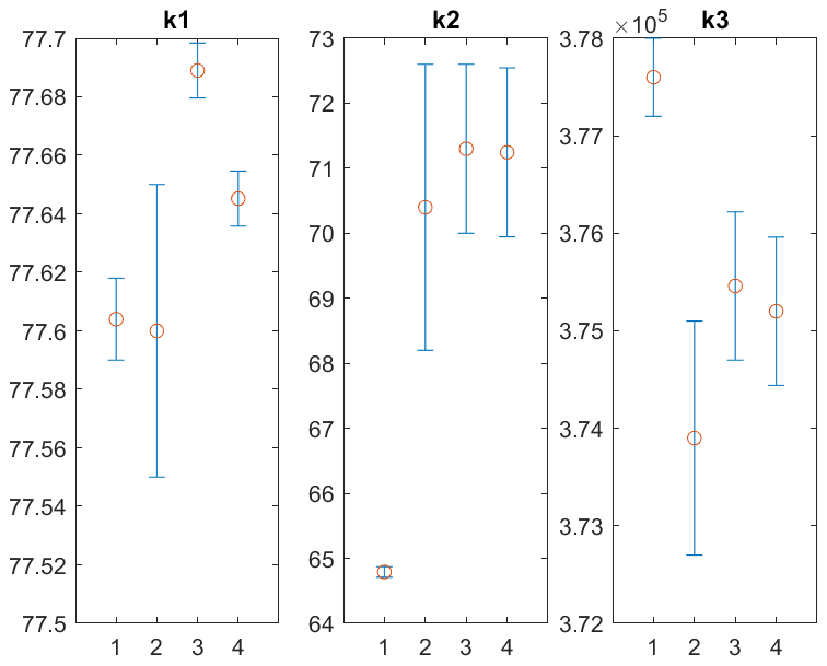
Table A1 List of DOIs associated with the UNAVCO GNSS stations from which RINEX data have been used in this study.

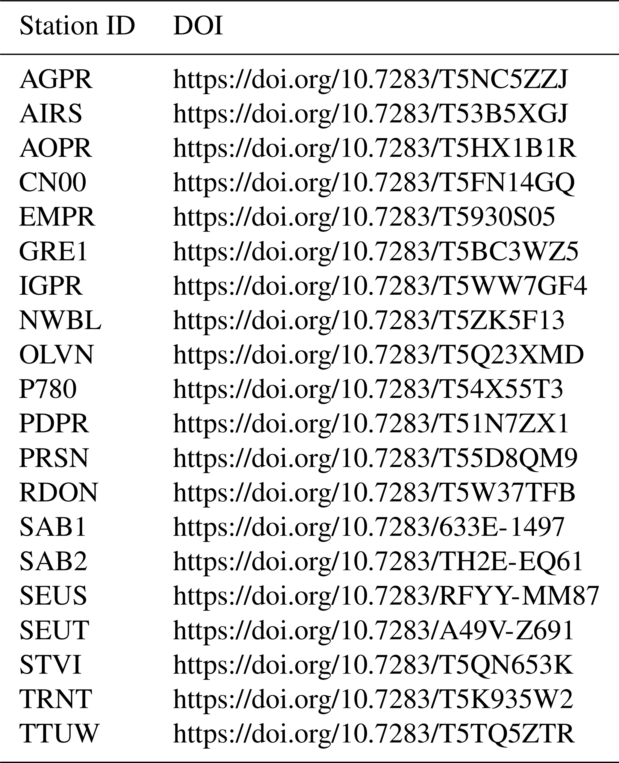
We start with Rueger (2002)'s “best average” coefficients $k_{\mathrm{1}}^{\prime }=\mathrm{77.6681}$ K hPa⁻¹, k₂=71.2952 K hPa⁻¹, k₃=375 463 K² hPa⁻¹, k₄=133.4800 K hPa⁻¹, where k₄ is the refractivity constant for CO₂ and $k_{\mathrm{1}}^{\prime }$ it the refractivity constant for dry air without CO₂. Using a present-day CO₂ mixing ratio of r_c=408 ppm, $k_{\mathrm{1}}^{\prime }$ and k₄ can be summed together to form k₁, the refractivity constant for dry air including CO₂, $k_{\mathrm{1}}=k_{\mathrm{1}}^{\prime }\cdot (\mathrm{1}-r_{\mathrm{c}})+k_{\mathrm{4}}\cdot r_{\mathrm{c}}$, to give k₁=77.6909 K hPa⁻¹. The last step is correcting for the non-ideal gas effects using the compressibility factor given by Owens (1967), i.e. $\mathrm{1}/Z_{\mathrm{d}}=\mathrm{1.000588}$ for dry air at 273.15 K and 1013.25 hPa, and $\mathrm{1}/Z_{\mathrm{w}}=\mathrm{1.000698}$ for water vapour at 293.15 K and a partial pressure of 13.33 hPa (the conditions of measurements of refractivity used by Rueger, 2002). Finally, the updated refractivity coefficients become

• $k_{\mathrm{1}}=\mathrm{77.6452}\pm \mathrm{0.0094}$ K hPa⁻¹

• $k_{\mathrm{2}}=\mathrm{71.2}\pm \mathrm{1.3}$ K hPa⁻¹

• $k\mathrm{3}=(\mathrm{3.7520}\pm \mathrm{0.0076})\times {\mathrm{10}}^{\mathrm{5}}$ K² hPa⁻¹,

where we included the uncertainties evaluated by Rueger (2002). If we assume that these uncertainties are fair estimates of the true absolute accuracy of the coefficients, the uncertainty in the IWV estimates due to k₁, k₂, and k₃, would be 0.04, 0.03, and 0.06 kg m⁻², respectively, under the average conditions of EUREC⁴A (IWV = 32 kg m⁻²). The systematic bias due to the uncertainty in the refractivity coefficients is thus extremely small. However, using the new estimates can make some systematic difference compared to those used in past studies.

Figure A1 compares the new refractivity coefficients to those from Thayer (1974) and Bevis et al. (1994), which are the two most widely used data sources in GNSS meteorology, and those from Rueger (2002) (without the compressibility factor correction and assuming a CO₂ mixing ratio of 375 ppm). It is seen that the k₁ from Rueger is about 0.09 K hPa⁻¹ larger than those from Thayer (1974) and Bevis et al. (1994), and that the new value differs only by 0.04 K hPa⁻¹ from the latter which represents a ZHD difference of 1.22 mm and a IWV difference of −0.19 kg m⁻² (the negative sign is because a larger ZHD correction decreases the IWV estimate). The new value for k₂ is in agreement with Bevis et al. (1994) and Rueger (2002), but this coefficient has a small weight in the final IWV estimate anyway. The new value for k₃ is in good agreement with Rueger (2002) and to a lesser extent with Thayer (1974) and Bevis et al. (1994), from which it differs by −0.2399 and $+\mathrm{0.1301}\times {\mathrm{10}}^{\mathrm{5}}$ K² hPa⁻¹, respectively, leading to a small fractional change in IWV of −0.64 % (−0.20 kg m⁻²) and +0.35 % (+0.11 kg m⁻²), where the IWV biases in kg m⁻² are computed assuming a mean value of IWV = 32 kg m⁻².

In conclusion, based on the differences between published refractivity coefficients and their uncertainties, we consider that the uncertainty in the absolute IWV values (i.e. the possible bias) retrieved from GNSS during EUREC⁴A due to these coefficients is at the level of ±0.2 kg m⁻².