the Creative Commons Attribution 4.0 License.
the Creative Commons Attribution 4.0 License.
 | 28 May 2021
The consolidated European synthesis of CO2 emissions and removals for the European Union and United Kingdom: 1990–2018
Ana Maria Roxana Petrescu
Matthew J. McGrath
Robbie M. Andrew
Philippe Peylin
Glen P. Peters
Philippe Ciais
Gregoire Broquet
Francesco N. Tubiello
Christoph Gerbig
Julia Pongratz
Greet Janssens-Maenhout
Giacomo Grassi
Gert-Jan Nabuurs
Pierre Regnier
Ronny Lauerwald
Matthias Kuhnert
Juraj Balkovič
Mart-Jan Schelhaas
Hugo A. C. Denier van der Gon
Efisio Solazzo
Chunjing Qiu
Roberto Pilli
Igor B. Konovalov
Richard A. Houghton
Dirk Günther
Lucia Perugini
Monica Crippa
Raphael Ganzenmüller
Ingrid T. Luijkx
Pete Smith
Saqr Munassar
Rona L. Thompson
Giulia Conchedda
Guillaume Monteil
Marko Scholze
Ute Karstens
Patrick Brockmann
Albertus Johannes Dolman
Reliable quantification of the sources and sinks of atmospheric carbon dioxide (CO2), including that of their trends and uncertainties, is essential to monitoring the progress in mitigating anthropogenic emissions under the Kyoto Protocol and the Paris Agreement. This study provides a consolidated synthesis of estimates for all anthropogenic and natural sources and sinks of CO2 for the European Union and UK (EU27 + UK), derived from a combination of state-of-the-art bottom-up (BU) and top-down (TD) data sources and models. Given the wide scope of the work and the variety of datasets involved, this study focuses on identifying essential questions which need to be answered to properly understand the differences between various datasets, in particular with regards to the less-well-characterized fluxes from managed ecosystems. The work integrates recent emission inventory data, process-based ecosystem model results, data-driven sector model results and inverse modeling estimates over the period 1990–2018. BU and TD products are compared with European national greenhouse gas inventories (NGHGIs) reported under the UNFCCC in 2019, aiming to assess and understand the differences between approaches. For the uncertainties in NGHGIs, we used the standard deviation obtained by varying parameters of inventory calculations, reported by the member states following the IPCC Guidelines. Variation in estimates produced with other methods, like atmospheric inversion models (TD) or spatially disaggregated inventory datasets (BU), arises from diverse sources including within-model uncertainty related to parameterization as well as structural differences between models. In comparing NGHGIs with other approaches, a key source of uncertainty is that related to different system boundaries and emission categories (CO2 fossil) and the use of different land use definitions for reporting emissions from land use, land use change and forestry (LULUCF) activities (CO2 land). At the EU27 + UK level, the NGHGI (2019) fossil CO2 emissions (including cement production) account for 2624 Tg CO2 in 2014 while all the other seven bottom-up sources are consistent with the NGHGIs and report a mean of 2588 (± 463 Tg CO2). The inversion reports 2700 Tg CO2 (± 480 Tg CO2), which is well in line with the national inventories. Over 2011–2015, the CO2 land sources and sinks from NGHGI estimates report −90 Tg C yr−1 ± 30 Tg C yr−1 while all other BU approaches report a mean sink of −98 Tg C yr−1 (± 362 Tg of C from dynamic global vegetation models only). For the TD model ensemble results, we observe a much larger spread for regional inversions (i.e., mean of 253 Tg C yr−1 ± 400 Tg C yr−1). This concludes that (a) current independent approaches are consistent with NGHGIs and (b) their uncertainty is too large to allow a verification because of model differences and probably also because of the definition of “CO2 flux” obtained from different approaches. The referenced datasets related to figures are visualized at https://doi.org/10.5281/zenodo.4626578 (Petrescu et al., 2020a).


Global atmospheric concentrations of CO2 have increased 46 % since pre-industrial times (pre-1750) (WMO, 2019). The rise of CO2 concentrations in recent decades is caused primarily by CO2 emissions from fossil sources. Globally, fossil emissions grew at a rate of 1.3 % yr−1 for the decade 2009–2018 and accounted for 87 % of the anthropogenic sources in the total carbon budget (Friedlingstein et al., 2019). In contrast, global CO2 emissions from land use and land use change estimated from bookkeeping models and dynamic global vegetation models (DGVMs) were approximately stable during the same period, albeit with large uncertainties (Friedlingstein et al., 2019).
National greenhouse gas inventories (NGHGIs) are prepared and reported under the UNFCCC on an annual basis by Annex I countries1, based on IPCC Guidelines using national activity data and different levels of sophistication (tiers) for well-defined sectors. These inventories contain time series of annual greenhouse gas (GHG) emissions from the 1990 base year2 until 2 years before the current year and were required by the UNFCCC and used to track progress towards countries' reduction targets under the Kyoto Protocol (UNFCCC, 1997). The IPCC tiers represent the level of sophistication used to estimate emissions, with Tier 1 based on global or regional default values, Tier 2 based on country- and technology-specific parameters, and Tier 3 based on more detailed process-level modeling. Uncertainties in NGHGIs are calculated based on ranges in observed (or estimated) emission factors and variation of activity data, using the error propagation method (95 % confidence interval) or Monte Carlo methods, based on clear guidelines (IPCC, 2006).
NGHGIs follow principles of transparency, accuracy, consistency, completeness and comparability (TACCC) under the guidance of the UNFCCC (2014). Methodological procedures follow the 2006 IPCC Guidelines (IPCC, 2006) and can be upgraded and completed with the IPCC 2019 Refinement (IPCC, 2019) containing updated sectors and additional sources. Atmospheric GHG concentration data can be used to derive estimates of the GHG fluxes based on atmospheric transport inverse modeling techniques (Rayner et al., 2019). Such estimates are often called top-down (TD) estimates since these are based on the analysis of concentrations, which represent the sum of the effects of sources and sinks, in contrast to bottom-up (BU) estimates, which rely on models analyzing the processes causing the fluxes. Current UNFCCC procedures do not require observation-based evidence in the NGHGI and do not incorporate independent, large-scale-observation-based GHG budgets, but the latest guidelines allow the use of atmospheric data for external checks within the data quality control, quality assurance and verification process (2006 IPCC Guidelines, chap. 6: QA/QC procedures). Only a few countries (e.g., Switzerland, UK, New Zealand and Australia) use atmospheric observations on a voluntary basis to complement their national inventory data with top-down estimates annexed to their NGHGI (Bergamaschi et al., 2018).
For the post-2020 reporting (which will start in 2023 for the inventory of year 2021), the Paris Agreement follows on the Kyoto Protocol, and, at the EU level, the GHG monitoring mechanism Regulation 525 (2013) is replaced by Regulation 1999 (2018), while Regulation 824 (2018) embeds the LULUCF sector with estimates based on spatial information in the EU climate targets of 2030. A key element in the current policy process is to facilitate the global stocktake exercise of the UNFCCC foreseen in 2023, which will assess collective progress towards achieving the near- and long-term objectives of the Paris Agreement, also considering mitigation, adaptation and means of implementation. The global stocktake is expected to create political momentum for enhancing commitments in nationally determined contributions (NDCs) under the Paris Agreement.
Key components of the global stocktake are the NGHGI submitted by countries under the enhanced transparency framework of the Paris Agreement. Under the new framework, for the first time, developing countries will be required to submit their inventories on a biennial basis, alongside developed countries that will continue to submit their inventories and full time series on an annual basis. This calls for robust and transparent approaches that can build up long-term emission compilation capabilities and be applied to different situations. A priority is to refine estimates of CH4 and N2O emissions, which are more uncertain than the CO2 fossil emissions. Fossil CO2 emissions are closely anchored to well-established fuel use statistics with narrow uncertainty ranges on emissions factors, while CO2 from LULUCF and CH4 and N2O have highly uncertain activity data and/or emission factors (see companion paper, Petrescu et al., 2021). However, CO2 emissions dominate the GHG fluxes, and there is need for monitoring and verification support capacity (Janssens-Meanhout et al., 2020) as the reduction of anthropogenic CO2 fluxes becomes increasingly important for the climate negotiations of the Paris Agreement and where observation-based data can provide information on the actual situation. In addition, while fossil CO2 emissions are known to relatively high precision, LULUCF activities are generally much more uncertain (RECCAP, https://www.globalcarbonproject.org/Reccap/index.htm, last access: November 2020, CarboEurope, http://www.carboeurope.org/, last access: November 2020) and as described below in Sects. 2.2. and 3.2.
The current study presents consistently derived estimates of CO2 fluxes from BU and TD approaches for the EU27 and UK, building partly on Petrescu et al. (2020b) for the LULUCF sector and on Andrew (2020) for fossil sectors while laying the foundation for future annual updates. Every year (time t) the Global Carbon Project (GCP) in its Global Carbon Budget (GCB) quantifies large-scale CO2 budgets up to year t−1, bringing in information from global to large latitude bands, including various observation-based flux estimates from BU and TD approaches (Friedlingstein et al., 2020). Except for two sector-specific BU models based on national statistics (EFISCEN and CBM), we note that the BU observation-based approaches used in the GCB and in this paper are based on the NGHGI estimates provided by national inventory agencies to the UNFCCC with differences coming from allocation. They rely heavily on statistical data combined with Tier 1 and Tier 2 approaches. In our case, focusing on a region that is well covered with data and models (Europe), BU also refers to Tier 3 process-based models or complex bookkeeping models (see Sect. 2). At regional and country scales, no systematic and regular comparison of these observation-based CO2 flux estimates with reported fluxes at UNFCCC is yet feasible. As a first step in this direction, within the European project VERIFY (http://verify.lsce.ipsl.fr/, last access: February 2021), the current study compares observation-based flux estimates of BU versus TD approaches and compares them with NGHGIs for the EU27 + UK and five sub-regions (Fig. 4). The methodological and scientific challenges to compare these different estimates have been partly investigated before (Grassi et al., 2018a, for LULUCF; Peters et al., 2009, for fossil sectors) but not in a systematic and comprehensive way including both fossil and land-based CO2 fluxes.
The work presented here represents many distinct datasets and use of models in addition to the individual country submissions to the UNFCCC for all European countries, which while following the general guidance laid out in IPCC (2006) still differ in specific approaches, models and parameters, in addition to differences in underlying activity datasets. A comprehensive investigation of detailed differences between all datasets is beyond the scope of this paper, though attempts have been previously made for specific subsectors (Petrescu et al., 2020b, for AFOLU3; Federici et al., 2015, for FAOSTAT versus NGHGIs). As this is the most comprehensive comparison of NGHGIs and research datasets (including both bottom-up (BU) and top-down (TD) approaches) for Europe to date, we focus here on a set of questions that such a comparison raises. How can one fairly compare the detailed sectoral NGHGIs to observation-based estimates? What new information do the observation-based estimates provide, for instance on the mean fluxes, spatial disaggregation, trends and inter-annual variation? What can one expect from such complex studies, where are the key knowledge gaps, what is the added value to policy makers and what are the next steps to take?
We compare official anthropogenic NGHGI emissions with research datasets correcting wherever needed research data on total emissions/sinks to separate out anthropogenic emissions. We analyze differences and inconsistencies between emissions and sinks and make recommendations towards future actions to evaluate NGHGI data. While NGHGIs include uncertainty estimates, special disaggregated research datasets of emissions often lack quantification of uncertainty. While this is also a call to those developers to associate more detailed uncertainty estimates with their products, here we use the median and minimum/maximum (min/max) range of different research products of the same type to get a first estimate of overall uncertainty. Table A2 in Appendix A presents the methodological differences of current study with respect to Petrescu et al. (2020b).
We use data of the total CO2 emissions and removals from the EU27 + UK from TD inversions and BU estimates, in addition to BU estimates from sector-specific models. We collected data of CO2 fossil and CO2 land4 emissions and removals between 1990 and 2018 (or the last available year if the datasets do not extend to 2018) from peer-reviewed literature and other data delivered under the VERIFY project (see description in Appendix A). The detailed data source descriptions are found in Sect. A1 and A2. For the BU anthropogenic CO2 fossil estimates we used global inventory datasets (Emissions Database for Global Atmospheric Research (EDGAR v5.0.), Food and Agriculture Organization Corporate Statistical Database (FAOSTAT), British Petroleum (BP), Carbon Dioxide Information Analysis Center (CDIAC), GCP, Energy Information Administration (EIA), International Energy Agency (IEA); see Table 1) described in detail by Andrew (2020), while for CO2 land estimates we used BU research-level biogeochemical models (e.g., DGVMs TRENDY-GCP, bookkeeping models; see Table 2). For TD we used global inversions (from the GCP in Friedlingstein et al., 2019) as well as regional inversions at higher spatial resolution (CarboScopeReg, EUROCOM, Monteil et al., 2020; Konovalov et al., 2016).
The values are defined from an atmospheric perspective: positive values represent a source to the atmosphere and negative ones a removal from the atmosphere. As an overview of potential uncertainty sources, Appendix B presents the use of emission factor (EF) data, activity data (AD), and, whenever available, uncertainty methods used for all CO2 land data sources used in this study. The referenced data used for the figures' replicability purposes are available for download at https://doi.org/10.5281/zenodo.4626578 (Petrescu et al., 2020a). We focus herein on the EU27 and the UK. Within the VERIFY project, we have in addition constructed a web tool which allows for the selection and display of all plots shown in this paper (as well as the companion paper on CH4 and N2O, Petrescu et al., 2021) not only for the regions shown here but for a total of 79 countries and groups of countries in Europe. The website, located on the VERIFY project website (http://webportals.ipsl.jussieu.fr/VERIFY/FactSheets/, last access: February 2021), is accessible with a username and password distributed by the project. Figure 4 includes also data from countries outside the EU but located within geographical Europe (Switzerland, Norway, Belarus, Ukraine and Republic of Moldova).
2.1 CO2 anthropogenic emissions from NGHGIs
UNFCCC NGHGI (2019) emissions are country estimates covering the period 1990–2017. The Annex I Parties to the UNFCCC are required to report emissions inventories annually using the common reporting format (CRF). This annual published dataset includes all CO2 emissions sources for those countries and for most countries for the period 1990 to t−2. Some eastern European countries' submissions begin in the 1980s. Revisions are made on an irregular basis outside of the standard annual schedule.
2.2 CO2 fossil emissions
CO2 fossil emissions occur when fossil carbon compounds are broken down via combustion or other forms of oxidation or via non-metal processes such as for cement production. Most of these fossil compounds are in the form of fossil fuels, such as coal, oil and natural gas. Another category is fossil carbonates, such as calcium carbonate and magnesium carbonate, which are used as feed stocks in industrial processes and whose decomposition also leads to emissions of CO2. Because CO2 fossil emissions are largely connected with energy, which is a closely tracked commodity group, there is a wealth of underlying data that can be used for estimating emissions. However, differences in collection, treatment, interpretation and inclusion of various factors such as carbon contents and fractions of oxidized carbon lead to methodological differences (Appendix A, Table A1) resulting in differences of emissions between datasets (Andrew, 2020). In contrast to BU estimates, atmospheric inversions for emissions of fossil CO2 are not fully established (Brophy et al., 2019), though estimates exist. The main reason is that the types of atmospheric networks suitable for fossil CO2 atmospheric inversions have not been widely deployed yet (Ciais et al., 2015).
In this analysis, the BU CO2 fossil estimates are presented and split per fuel type and reported for the last year when all data products are available (Andrew, 2020). In addition to the BU CO2 fossil estimates, we report a fossil fuel CO2 emission estimate for the year 2014 from a 4-year inversion assimilating satellite observations. In order to overcome the lack of CO2 observation networks suitable for the monitoring of fossil fuel CO2 emissions at a national scale, this inversion is based on atmospheric concentrations of co-emitted species. It assimilates satellite CO and NO2 data. While the spatial and temporal coverage of these CO and NO2 observations is large, the conversion of the information on these co-emitted species into fossil fuel CO2 emission estimates is complex and carries large uncertainties. Therefore, we focus here on the comparison between the uncertainties in the inversion versus the magnitude and variations of BU estimates without discussing system boundaries and constraints of each of these products (which are instead discussed in Andrew, 2020). The detailed descriptions of each of the data products described in Table 1 are found in Appendix A1.
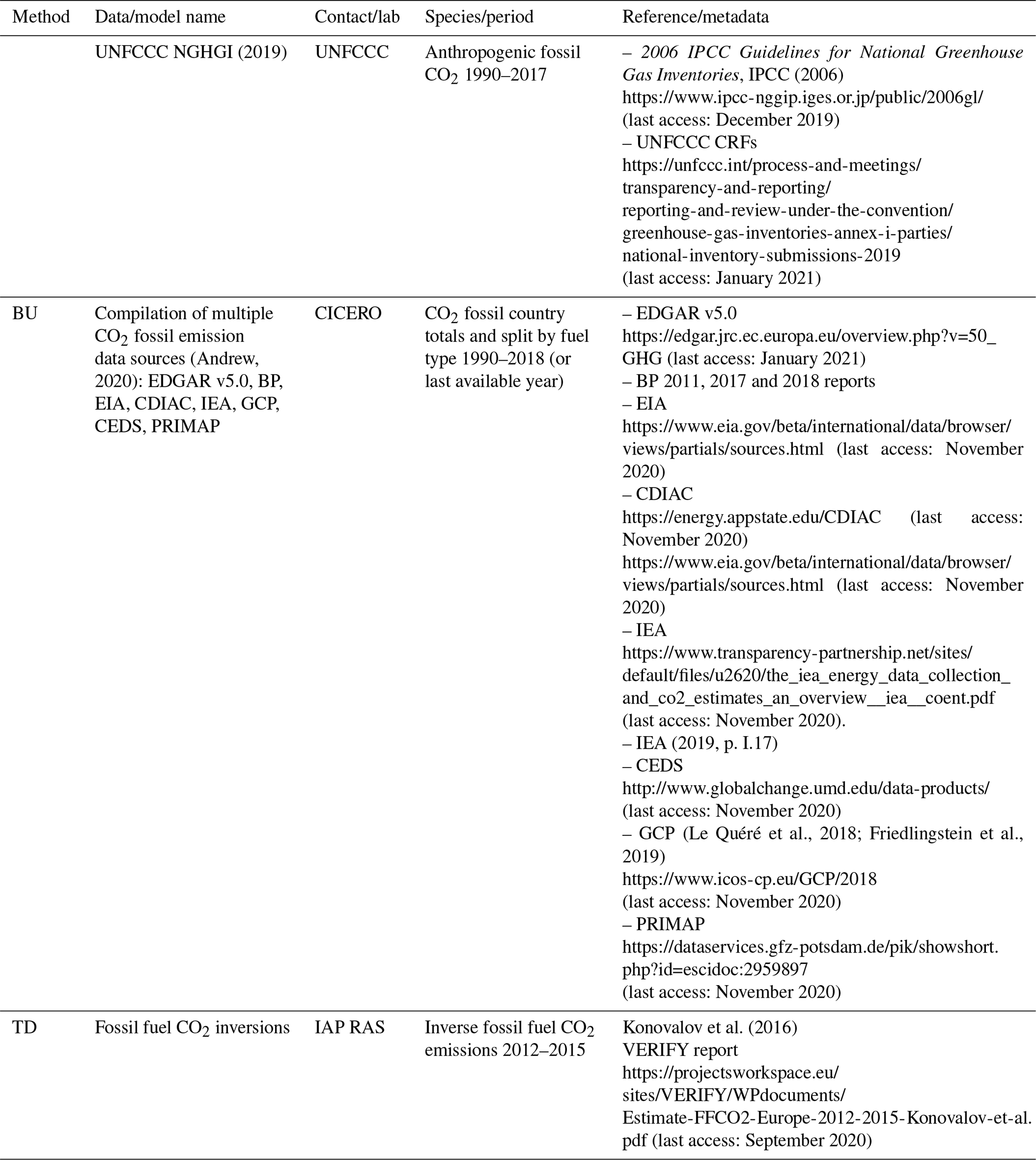
Table 1Data sources for the anthropogenic CO2 fossil emissions included in this study.
2.3 CO2 land fluxes
CO2 land fluxes include CO2 emissions and removals from LULUCF activities, based on either BU or TD CO2 estimates from inversion ensembles, represented by the data sources and products described in Table 2. We compare CO2 net emissions from the LULUCF sector primarily from three land use classes5 (forest land, cropland and grassland) from both land class remaining6 (land class remains unchanged) and land class converted7 (land class changed in the last 20 years). The wetlands, settlements and other land categories are included in the discussion on total LULUCF activities (including harvested wood products, HWPs) presented in Sect. 3.3.1, 3.3.3 and 3.3.4. Not all the classes reported to the UNFCCC are present in FAOSTAT or other models; in addition some models are sector-specific. We use the notation of “FL-FL”, “CL-CL” and “GL-GL” to indicate forest, cropland and grassland which remain in the same class from year to year. We present separate results from sector-specific models reporting carbon fluxes for FL-FL, CL-CL and GL-GL (the models EPIC-IIASA, ECOSSE, EFISCEN, CBM), those including multiple land use sectors and simulating land use changes (e.g., dynamic global vegetation models (DGVMs), ensemble TRENDY v7 (Sitch et al., 2008; Le Quéré et al., 2009)), and those employing bookkeeping approaches (H&N, Houghton and Nassikas, 2017; and BLUE, Hansis et al., 2015). The detailed description of each of the products described in Table 3 is found in Appendix A2.
The two inverse model ensembles presented here are the GCB 2018 for 1990–2018 (Le Queré et al., 2018) and EUROCOM for 2006–2015 (Monteil et al., 2020). The GCB inversions are global and include CarbonTracker Europe (CTE; van der Laan-Luijkx et al., 2017), CAMS (Chevallier et al., 2005) and the Jena CarboScopeReg (Rödenbeck, 2005). The EUROCOM inversions are regional, with a domain limited to Europe and higher-spatial-resolution atmospheric transport modes, with five inversions covering the entire period 2006-2015 as analyzed in Monteil et al. (2019). They report net ecosystem exchange (NEE) fluxes. These inversions make use of more than 30 atmospheric observing stations within Europe, including flask data and continuous observations, and work at typically higher spatial resolution than the global inversion models. The other regional inversion presented here is generated with the CarboScopeReg (CSR) inversion system (2006–2018), with different ensemble members. This system is part of the EUROCOM ensemble, but new runs were carried out for the VERIFY project. The results are plotted separately to illustrate two points: (1) that the CSR runs for VERIFY are not identical to those submitted to EUROCOM (VERIFY runs from CSR included several sites that started shortly before the end of the EUROCOM inversion period) and (2) that the CSR model was used in four distinct runs in VERIFY, which differ in the spatial correlation of prior uncertainties and in the number of atmospheric stations whose observations are assimilated. By presenting CSR separate from the EUROCOM results, one can get an idea of the uncertainty due to various model parameters in one inversion system, with one single transport model.
3.1 Overall NGHGI reported fluxes
According to UNFCCC NGHGI (2019) estimates, in 2017 the European Union (EU27 + UK) emitted 3.96 Gt CO2 eq. from all sectors (including LULUCF) and 4.21 Gt CO2 eq. (excluding LULUCF) (Appendix B1, Fig. B1a). LULUCF only contributed 0.28 Gt CO2 in 2017. This number is consistent with a variety of independent emission inventories (Andrew, 2020; Petrescu et al., 2020b). A few large economies account for the largest share of EU27 + UK emissions, with Germany, the UK and France representing 43 % of the total CO2 emissions (excluding LULUCF) in 2017. For LULUCF the countries reporting the largest CO2 sinks were Sweden, Poland and Spain, accounting for 45 % of the overall EU27 + UK sink strength. Only a few countries (the Netherlands, Ireland, Portugal and Denmark) reported a net LULUCF source in 2017; in the case of Portugal, this was mainly due to emissions from biomass burning. The UNFCCC shows minimal inter-annual variability, so the 2017 values are indicative of longer-term trends.
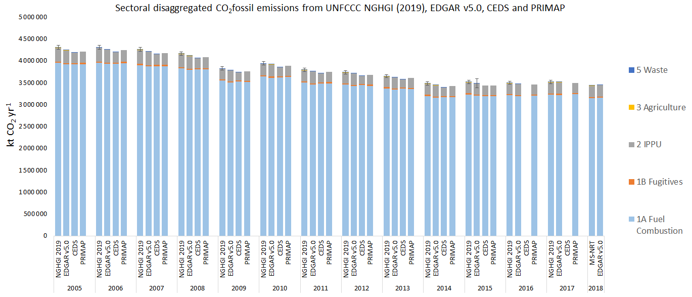
Figure 1Total sectoral breakdown of CO2 fossil emissions from UNFCCC NGHGI (2019), EDGAR v5.0, CEDS and PRIMAP. Subsectors 1A and 1B belong to the energy sector. The total UNFCCC uncertainty is 1.4 % and was calculated based on the UNFCCC NGHGI (2018) submissions. EDGAR v5.0 uncertainties were calculated only for the year 2015 using a lognormal distribution function and ranged from a minimum of 3 % to a maximum of 4 %.
CO2 fossil emissions are dominated by the energy sector, combustion and fugitives, representing 91.4 % of the total EU27 + UK CO2 emissions (excluding LULUCF) or 3.25 Gt CO2 yr−1 in 2017. The industrial process and product use sector (IPPU) sector contributes 8.2 % or 0.2 Gt CO2 yr−1, while the CO2 emissions reported as part of the agriculture sector cover only liming and urea application – UNFCCC sectors 3G and 3H8 respectively. Together with waste, in 2017, the emissions from agriculture represent 0.4 % of the total UNFCCC CO2 emissions. Often, the NGHGI reported values for CO2 emissions do not include LULUCF as these reported emissions are inherently uncertain, showing almost no inter-annual variability, contrary to observation-based BU approaches (e.g., process-based models) which do show large inter-annual variations as a result of inter-annual variability in climatic conditions and (in part as a consequence of this variability) in the occurrence of natural disturbances (Kurz, 2010; Olivier et al., 2017).
3.2 CO2 fossil emissions
3.2.1 Bottom-up estimates by sector
At the EU27 + UK level our results show that CO2 fossil emissions are consistent between UNFCCC NGHGI (2019) and BU inventories from EDGAR v5.0, CEDS and PRIMAP. EDGAR v5.0 reports the same sources as the UNFCCC, but CEDS reports emissions from energy (1A+1B), IPPU and waste up to 2014, and PRIMAP reports emissions only for energy and IPPU. All BU datasets show a good match for overlapping sectors, energy and IPPU (Fig. 1, sum of subsectors 1A and 1B).
CO2 fossil emissions are dominated by the energy sector, which includes emissions from energy use in energy industries (heat and electricity, industry, transport and buildings). Out of the remaining three sectors (IPPU, agriculture and waste), IPPU contributes the most to the CO2 emissions; in the EU27 + UK these emissions contributed 7.1 %, 7.5 %, 5.6 % and 6.4 % from the total NGHGIs, EDGAR v5.0 (2017), CEDS (2014) and PRIMAP (2015) respectively. For agriculture and waste, overall, emissions are very small, accounting in the EU27 + UK in 2017 for 0.3 % (NGHGIs) and 0.4 % (EDGAR v5.0) respectively; therefore this difference is negligible for the total C budget.
3.2.2 Bottom-up estimates by source category
While Fig. 1 was made to assist explanation of differences between datasets disaggregated by sector (e.g., energy industry, transport), in Fig. 2 we present CO2 fossil emissions results from the EU27 + UK split by major source categories (solid, liquid, gas). As in Andrew (2020), we observe good agreement between all data sources and UNFCCC NGHGI (2019) data at this level of regional aggregation. The figure presents estimates for the year 2014, as that was the most recent year when all sources reported estimates. BP9 (2018), CEDS (v_2019_12_23) and EDGAR10 v5.0 (2020) do not publish emissions split by fuel type at the country level, and the latter two are shown as dark grey, while the former is shown separating gas from liquid/solid.
While the datasets agree well, there are some differences. The EIA (2020) estimate is higher than others, largely because it includes international bunker fuels in liquid-fuel emissions. The IEA (2019) excludes a number of sources from non-energy use of fuels as well as all carbonates. GCP's total matches the NGHGIs exactly by design but remaps some of the fossil fuels used in non-energy processes from “others” to the fuel types used. BP, CEDS and EDGAR v5.0 all report total emissions very similar to the UNFCCC NGHGI (2019).

Figure 2EU27 + UK total CO2 fossil emissions, as reported by eight data sources: BP, EIA, CEDS, EDGAR v5.0, GCP, IEA, CDIAC and UNFCCC NGHGI (2019). This figure presents the split per fuel type for year 2014. “Others” represents other emissions in the UNFCCC's IPPU, and international bunker fuels are not usually included in total emissions at the sub-global level. Neither EDGAR (v5.0 FT2017) nor CEDS publish a breakdown by fuel type, so only the total is shown.
3.2.3 Top-down estimates
Figure 3 represents the first attempt to evaluate our single inversion of CO2 fossil emissions, based on satellite CO and NO2 measurements, against BU estimates. The particular inversion reported here provides emission totals for the EU1111 + Switzerland, and these exclude non-fossil fuel emissions (Konovalov et al., 2016; Konovalov and Lvova, 2018). This inversion estimate partly relies on information available from the BU emission inventories – EDGAR v4.3.2 for 2012 (http://edgar.jrc.ec.europa.eu/overview.php?v=432_GHG, last access: December 2020, http://edgar.jrc.ec.europa.eu/overview.php?v=432_AP, last access: December 2020) and CDIAC for 2012–2014 (http://cdiac.ess-dive.lbl.gov/trends/emis/overview_2014.html, last access: September 2020, Boden et al., 2017) – and is therefore not fully independent from BU CO2 fossil emission estimates. The estimate from the inversion, despite its uncertainty (2700 Tg CO2 (± 480 Tg CO2)), is comparable with the mean of the CO2 emissions from the NGHGIs in 2014 (2624 Tg CO2) and to mean of the other seven BU sources 2588 (± 463 Tg CO2). The TD estimate does not include CO2 emissions from cement production, while some bottom-up inventories include them. Cement emissions are known to constitute only a minor fraction (∼ 5 %) of the total fossil CO2 emissions in Europe (UNFCCC, 2019; Andrew, 2019; Friedlingstein et al., 2020) and can be disregarded in the given comparison.
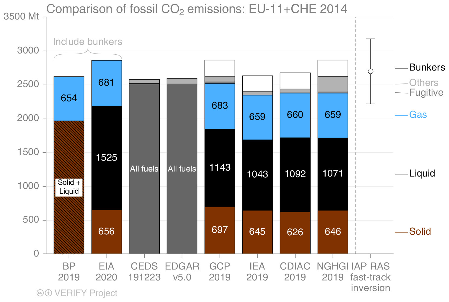
Figure 3A first attempt in comparing BU CO2 fossil estimates from eight datasets with a TD fast-track inversion (Konovalov and Lvova, 2018). The data represent the EU11 + Switzerland for the year 2014. The uncertainty bar on the inversions represents the 2σ confidence interval.
3.3 CO2 land fluxes
This section presents an update to the benchmark data collection by Petrescu et al. (2020b) on CO2 emissions and removals from the LULUCF sector (excluding energy-related emissions but including emissions from land use change, emissions from disturbances on managed land, and the natural sink on managed land), expanding the scope of that work by adding TD estimates from inverse model ensembles and additional BU models run with higher-resolution meteorological forcing data over the EU27 + UK.
Land CO2 fluxes result from CO2 emissions/removals from one land type converted to another (e.g., forests cleared for croplands), as well as emissions/removals from land occupied by terrestrial ecosystems (depending on the dataset, this may be from managed or unmanaged land, which complicates comparisons with NGHGIs). Such fluxes typically include emissions and sinks in soils and carbon shifts due to harvests, including emissions from the decay of harvested wood products (HWPs). Some estimates are specific to a given vegetation/sector type (i.e., only cropland or grassland). As discussed by Petrescu et al. (2020b), the analyzed fluxes therefore relate to emissions and removals from direct LULUCF activities (clearing of vegetation for agricultural purposes, regrowth after agricultural abandonment, wood harvesting and recovery after harvest, and management) but also indirect LULUCF for CO2 fluxes due to processes such as responses to environmental drivers (i.e., climate change and CO2 fertilization) on managed land12. Additional CO2 fluxes may occur on unmanaged land, but these fluxes are very small. According to national inventory reports (NIRs), all land in the EU27 + UK is considered managed, except for 5 % of France's territory.
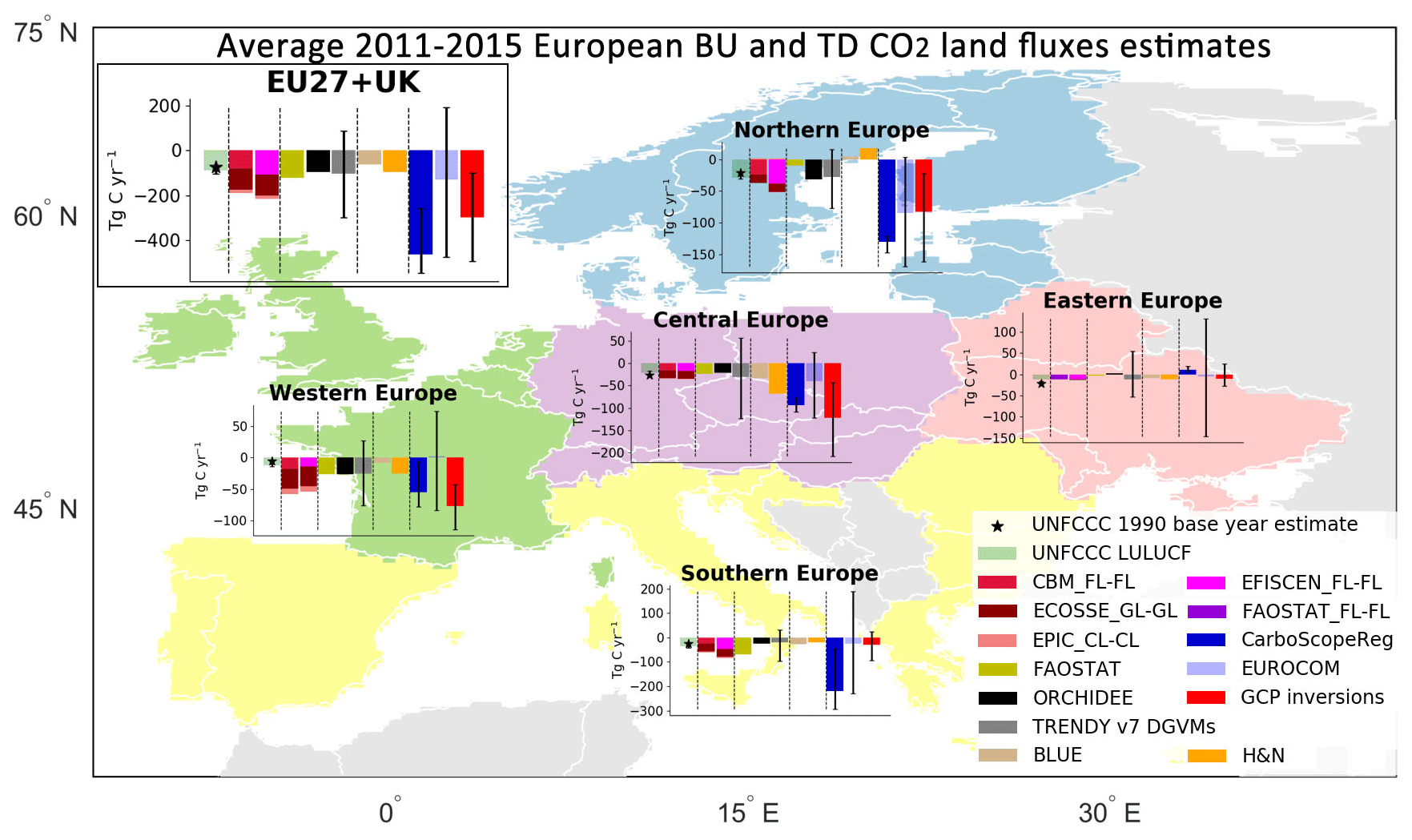
Figure 4Five-year-average (2011–2015) CO2 land flux estimates (in Tg C) for the EU27 + UK and five European regions (northern, western, central, southern and eastern non-EU). Eastern Europe does not include European Russia, and the UNFCCC uncertainty for the Republic of Moldova was not available. Northern Europe includes Norway. Central Europe includes Switzerland. The data are UNFCCC NGHGI (2019) submissions (grey) and base year 1990 (black star); four sector-specific BU models for FL-FL (CBM, EFISCEN), CL-CL (EPIC-IIASA) and GL-GL (ECOSSE); ecosystem models (ORCHIDEE and TRENDY v7 DGVMs); FAOSTAT; two bookkeeping models (BLUE and H&N), TD inversion ensembles (GCP2018, EUROCOM); and one regional European inversion represented by CarboScopeReg.
The indirect CO2 fluxes on managed and unmanaged land are part of the land sink in the definition used in IPCC Assessment Reports or the Global Carbon Project's annual Global Carbon Budget (Friedlingstein et al., 2019), while the direct LULUCF fluxes are termed “net land use change flux”. Grassi et al. (2018a) have shown that the inclusion or exclusion of the indirect sink on managed land in LULUCF is a key reason for discrepancy between reporting and scientific definitions.
Several studies have already analyzed the European land carbon budget from different perspectives and over several time periods using GHG budgets from fluxes, inventories and inversions (Luyssaert et al., 2012); flux towers (Valentini et al., 2000); forest inventories (Liski et al., 2000; Pilli et al., 2017; Nabuurs et al., 2018); and IPCC Guidelines (Federici et al., 2015; Tubiello et al., 2021), in addition to the first benchmark data collection of BU estimates (Petrescu et al., 2020b).
Achieving the well-below-2 ∘C temperature goal of the PA requires, among other things, low-carbon energy technologies, forest-based mitigation approaches and engineered carbon dioxide removal (Grassi et al., 2018a; Nabuurs et al., 2017). Currently, the EU27 + UK reports a sink for LULUCF, and forest management will continue to be the main driver affecting the productivity of European forests for the next decades (Koehl et al., 2010). For the EU to meet its ambitious climate targets, it is necessary to maintain and even strengthen the LULUCF sink (COM(2020) 562). Forest management, however, can enhance (Schlamadinger and Marland, 1996) or weaken (Searchinger et al., 2018) this sink. Furthermore, forest management not only influences the sink strength but also changes forest composition and structure, which affects the exchange of energy with the atmosphere (Naudts et al., 2016) and therefore the potential of mitigating climate change (Luyssaert et al., 2018; Grassi et al., 2019). Meteorological extremes (made more likely through climate change) can also affect the efficiency of the sink (Thompson et al., 2020). Therefore, understanding the evolution of the CO2 land fluxes is critical to meet the goals set out in the Paris Agreement.
3.3.1 Estimates of European and regional total CO2 land fluxes
We present results of the total CO2 land fluxes from the EU27 + UK and five main regions in Europe: north, west, central, east (non-EU) and south. The countries included in these regions are listed in Appendix A, Table A1.
Figure 4 shows the total CO2 fluxes from NGHGIs for both the 1990 base year and mean of the 2011–2015 period. We aim with this period to bring together all information over a 5-year period for which values are known in 2018. In fact this can be seen as a reference for what we can achieve in 2023, the year of the first global stocktake, where for most UN Parties the reported inventories will be compiled only up to the year 2021. Given that the global stocktake is only repeated every 5 years, a 5-year average is clearly of interest.
The CO2 fluxes in Fig. 4 include direct and indirect LULUCF on managed land. The total UNFCCC estimates include the total LULUCF emissions and sinks (by the UNFCCC definition) belonging to all six IPCC land classes and HWPs (see Sect. 2.3, Appendix B1, Fig. B1b). We plot these and compare them with fluxes simulated with statistical global datasets, bookkeeping and biosphere models, sector-specific models, and inversion model ensembles. The error bar represents the variability in model estimates as the min and max values in the ensemble.
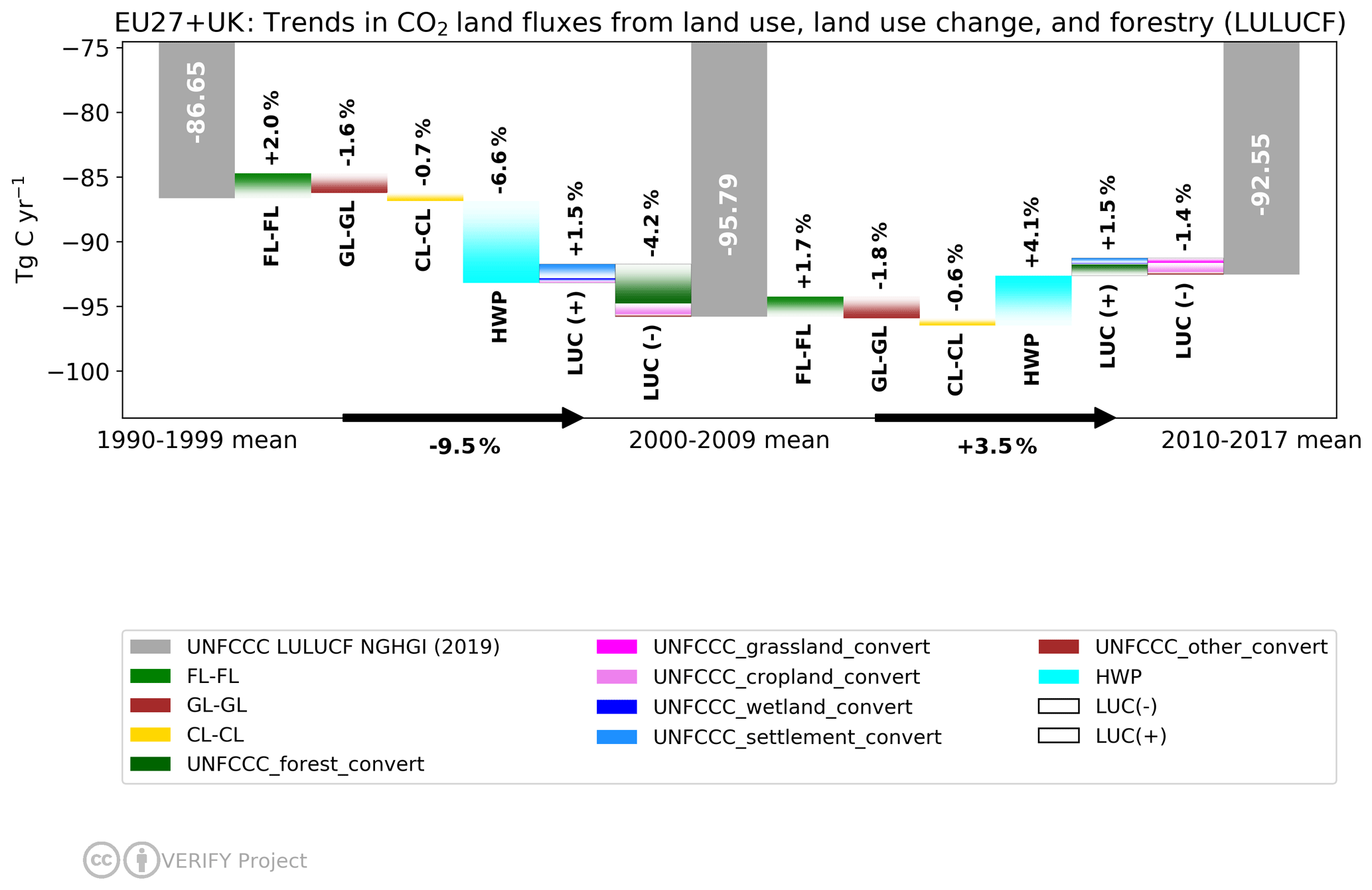
Figure 5The contribution of changes (%) in various LULUCF categories to the overall change in LULUCF multi-year mean emissions as reported by member states to the NGHGI UNFCCC (2019). Changes in land categories converted to other land are grouped to show net gains and net losses in the same column, with the bar color dictating which category each emission belongs to; note that the composition of the “LUC(+)” and “LUC(−)” bars can change between time periods. Not shown are emissions from “wetlands remaining wetlands”, “settlements remaining settlements” and “other land remaining other land” as none of the BU models used distinguish these categories. The fluxes follow the atmospheric convention, where negative values represent a sink while positive values represent a source.
For all regions and the EU27 + UK, we note considerable disagreement between the BU and TD results. We mostly see that BU (observation-based and process-based) estimates agree well with the NGHGIs, while inversions, in particular EUROCOM, report very strong sinks and high variability of the results compared to the BU estimates. We believe that, in general, the differences we see between regions' TD and BU results are linked to model-specific setups and definition issues explained in detail in Sect. 3.3.2 (process-based models and NGHGIs), Sect. 3.3.3 (DGVMs, bookkeeping models and NGHGIs) and Sect. 3.3.4 (all BU, TD and NGHGIs). As the current analysis is a first attempt to quantify EU27 + UK estimates as a whole, we aim in the future to deepen the analysis for regional/country results.
3.3.2 LULUCF CO2 fluxes from NGHGIs and decadal changes
In Fig. 5 we show the CO2 LULUCF flux decadal change from UNFCCC NGHGI (2019). The contribution of each category (“remaining” and “conversion”) to the overall reduction of CO2 emissions in percentages between the three mean periods (grey columns are the mean values over 1990–1999, 2000–2009 and 2010–2017). The “+” and the “−” signs represent a source and a sink to the atmosphere. LUC(−) represents the land use conversion changes that increase the strength of the LULUCF sink between two averages; LUC(+) represents the land use conversion changes that decrease the strength of the overall LULUCF sink. Note that the sectors inside LUC(−) may be sources or may be sinks, but between the two average periods, they become more negative. For the period between 1990–1999 mean and 2000–2009 mean the overall reduction is −9.5 % (i.e., increased land sink), with positive contribution from FL-FL and LUC(+) (wetlands, settlements and other land conversions) contributing to weakening the overall sink (+3.5 %)13 and with all others conversions contributing to the strengthening of the sink (−13 %)14. For the period between the 2000–2009 mean and the 2010–2017 mean we notice that the main contributors to the overall +3.5 % increase are FL-FL, HWPs and LUC(+) (forest, wetlands and settlement conversions), which contribute (+7.2 %) to weakening the sink, while GL-GL, CL-CL and LUC(−) (cropland, grassland and other conversions) contribute to strengthening the sink (−3.7 %).
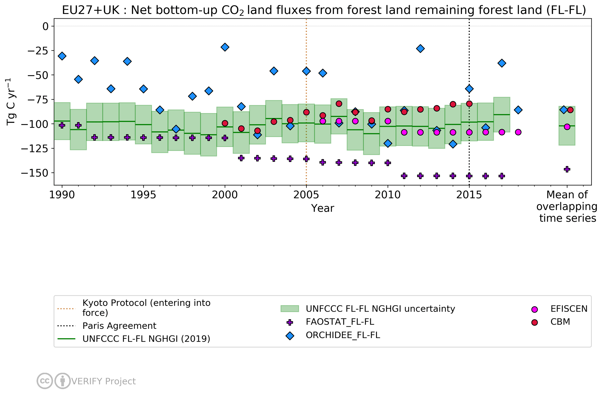
Figure 6Net CO2 land flux from forest land remaining forest land (FL-FL) estimates for the EU27 + UK CO2 from UNFCCC NGHGI 2019 submissions and bottom-up emission models with their 2006–2015 mean (on the right side). CBM FL-FL estimates include 25 EU and UK countries (excluding Cyprus and Malta); the relative error on the UNFCCC value represents the UNFCCC NGHGI (2018) MS-reported uncertainty computed with the error propagation method (95 % confidence interval) and is 19.6 % (with no values for Hungary and Cyprus). The negative values represent a sink.
We see that HWP emissions are by far the major contributor but in different directions across the two periods, from strengthening the sink between 1990–1999 and 2000–2009 to reducing the sink in the second period. This is mostly due to the specific accounting approach where a reduction on the amount of harvest, such as the one that occurred after the economic crisis in 2008, progressively reduced the inflow of raw material, and, taking into account the decay rate applied to each commodity, this further reduced the C stock within the same pool. Therefore, Fig. 5 suggests that carbon emissions from HWP decay became greater than the amount of carbon entering HWPs in recent decades.
3.3.3 Estimates of CO2 fluxes from bottom-up approaches
In this section we present annual total net CO2 land emissions between 1990–2018, i.e., induced by both LULUCF and other (environmental changes) processes from class-specific models as well as from models that simulate some or all classes. The definitions of the classes might differ from the definition of the LULUCF (FL, CL, GL etc.) (Figs. 6, 7 and 8), where, according to the 2006 IPCC Guidelines, to become accountable in the NGHGIs under remaining categories, a land use type must be in that class for at least 20 years. Over FL (both FL-FL and conversions) we compare modeled net biome productivity (NBP) estimates (including soil plus living and dead biomass C stock change) simulated with class-specific ecosystem models to UNFCCC and FAOSTAT data consisting of net carbon stock change in the living biomass pool (aboveground and belowground biomass) associated with forests and net forest conversion including deforestation.
The forest land estimates, which remain in this class (FL-FL) in Fig. 6, were simulated with ecosystem models (CBM, ORCHIDEE, EFISCEN) (described in Appendix A2 and Table B1), global datasets (FAOSTAT) and countries' official inventory statistics reported to UNFCCC. The results show that the differences between models are systematic, with CBM having slightly weaker sinks than EFISCEN and FAOSTAT. Starting with year 2000 and towards 2017, the FAOSTAT reports sinks that strengthen over time. Differences between estimates might be due to the use of different input data; e.g., CBM and EFISCEN use national forest inventory (NFI) data as the main source of input to describe the current structure and composition of European forest, while FAOSTAT uses input data directly from country submission done under the FAO Global Forest Resources Assessment (FRA, 201515) (e.g., carbon stock change calculated by FAO directly from carbon stocks and area data submitted by countries directly). Furthermore, FAOSTAT numbers include afforestation, i.e., the sum of all other land converted to FL, resulting in a smaller sink if afforestation would be removed, therefore matching the UNFCCC estimates better (Petrescu et al., 2020b).
For ORCHIDEE, the model shows a high inter-annual variability in carbon fluxes because ORCHIDEE operates on a sub-daily time step for most biogeochemical and biophysical processes except for a daily time step for “slow” processes like carbon allocation in the vegetation reservoirs, while all other models involved in this comparison use forest inventory data which are reported every few years (i.e., 5 years for FRA). ORCHIDEE results indicate that climatic perturbations and extreme events (multi-month droughts, in particular) can have significant impacts on the net carbon fluxes depending on when they occur. This is to some extent supported by dendrometer data, although highly varying per site and tree species, obscuring a significant net effect (Scharnweber et al., 2020). It should also be noted that dendrometer data measure carbon stored in individual trees, while the NBP reported in figures in this paper includes fluxes from litter and soil respiration. The variability of the weather data affects all components of the carbon dynamics in the ecosystems (hence NBP), with for instance impacts on C assimilation rates, length of the growing season, dynamics of respiration rates and allocation of the carbon in the plant (cf. Figs. 1 and 2 in Reichstein et al., 2013).
The UNFCCC NGHGI uncertainty of CO2 estimates for FL-FL across the EU27 + UK, computed with the error propagation method (95 % confidence interval) (IPCC, 2006), ranges between 23 % and 30 % when analyzed at the country level as it varies as a function of the component fluxes (NIR reports 2017, UNFCCC NGHGI, 2018). Given the different methodologies and input data for emission calculation and uncertainties in each method (10 Tg C yr−1 for the mean), we consider the match between the model EFISCEN and the UNFCCC NGHGI (2019) estimates to be good, in particular with respect to the similarity in temporal trends. The means of ORCHIDEE and CBM fall within the reported UNFCCC uncertainty (around 20 Tg C yr−1), while FAOSTAT lies outside of it. Note that FAOSTAT and EFISCEN have a different trend compared to other models and the NGHGIs.
Some of the reasons for differences between estimates we see in Fig. 6 are linked to different activity data (e.g., forest area) the models use, for example the stronger sink reported by FAOSTAT compared to the UNFCCC NGHGI. By analyzing three of the forest area products (ESA-CCI LUH2v2, Hurtt et al., 2020, used in ORCHIDEE, FAOSTAT and UNFCCC) we found the following.
-
For this study, the ORCHIDEE model used a so-called ESA-CCI LUH2v2 plant functional type (PFT) distribution (a combination of the ESA-CCI land cover map for 2015 with the historical land cover reconstruction from LUH2, Lurton et al., 2020) and assumes that the shrub land cover classes are equivalent to forest. In terms of area, the original ESA-CCI product corresponding to our domain of the EU-27 + UK shows shrub land equal to about 50 % of the tree area in 2015. A similar analysis using the FAOSTAT domain land cover, which maps and disseminates the areas of MODIS and ESA-CCI land cover classes to the SEEA land cover categories (http://www.fao.org/faostat/en/#data/LC, last access: June 2020), shows that shrub-covered areas are around 20 % of that of forested areas for the EU-27 + UK. The impact of classifying shrubs as “forests” on the total carbon fluxes could therefore account for a significant percentage of the differences between ORCHIDEE and other results in Fig. 6. ESA-CCI LUH2v2 does not include the 20-year transition period, as included in the IPCC reporting guidelines. This could be 1 % of the forests in Europe, but there is a considerable uncertainty in that based on the transition data seen between the maps.
-
FAOSTAT forest land area is based on country statistics from the FAO/FRA process and includes not only forest remaining forest area but all forested land, including afforestation.
Cropland and grassland (CL and GL) (in UNFCCC NGHGI, 2019, UNFCCC sectors 4B and 4C, respectively) include net CO2 emissions/removals from soil organic carbon (SOC) under remaining and conversion categories. Similar to forest land, we present in Fig. 7 the fluxes belonging to the remaining category CL-CL. The cropland definition in the IPCC includes cropping systems and agroforestry systems where vegetation falls below the threshold used for the forest land category, consistent with the selection of national definitions (IPCC glossary).
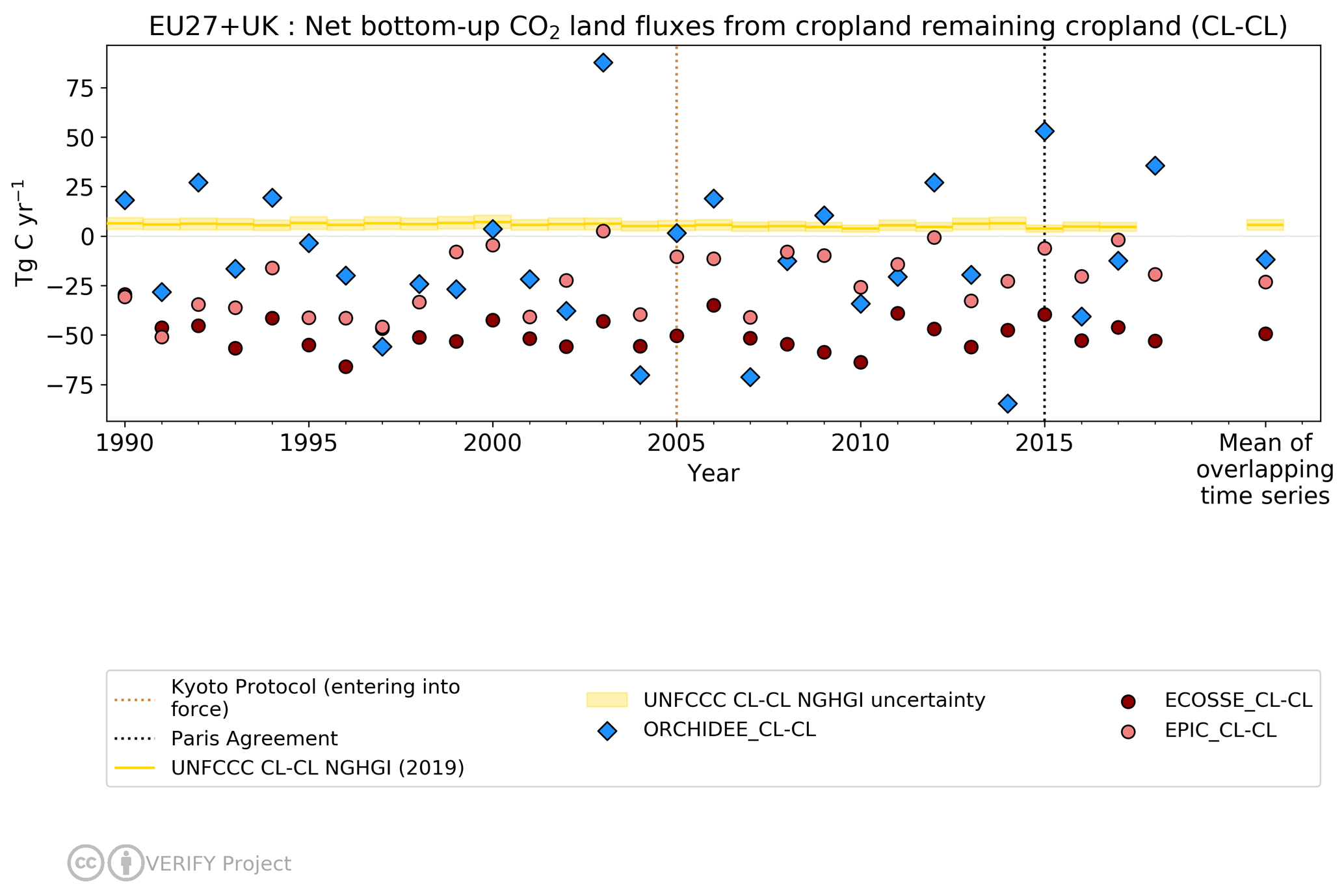
Figure 7Net CO2 flux from cropland remaining cropland estimates for the EU27 + UK from UNFCCC NGHGI (2019) submissions and bottom-up emission models with their 1990–2017 mean (on the right side). CL-CL emissions estimated with three ecosystem models: ORCHIDEE, ECOSSE and EPIC-IIASA. The relative error on the UNFCCC value represents the UNFCCC NGHGI (2018) MS-reported uncertainty computed with the error propagation method (95 % confidence interval) and is 47.5 % (with no data from Hungary, Cyprus and Portugal). The negative values represent a sink, while the positive values represent a source.
From Fig. 7 we see that modeled CL-CL inter-annual variabilities simulated by ECOSSE and EPIC-IIASA estimates are consistent, while ORCHIDEE shows a much larger year-to-year variation. The NGHGIs are mostly insensitive to inter-annual variability as the estimations are mainly based on statistical data for surfaces/activities and EFs that do not vary with changing environmental conditions.
The three process-based models report sinks in most years (means of −12, −49 and −23 Tg C respectively), contrary to the NGHGIs, which report a small but constant source over the whole period (mean of 5.6 ± 3.5 Tg C) with almost no inter-annual variability by construction. The source reported by NGHGIs, at the EU level, is mostly attributed to emissions from cropland on organic soils16 in the northern part of Europe which emit CO2 due to C oxidation from tillage activities. As an example, Finland and Sweden report together more than half of the total area of organic soil in Europe. Organic soils are an important source of emissions when they are under management practices that disturb the organic matter stored in the soil. In general, emissions from these soils are reported using country-specific values when they represent an important source within the total budget of GHG emissions. In the southern part of Europe, the two categories (CL-CL and GL-GL) are a sink, due to a lack of organic soils in those regions and due to an abandonment trend of land converting arable land to grassland (EU NIR, 2019). In addition, NGHGIs assume that all aboveground biomass of non-woody crops re-enters the atmosphere at harvest. In models like ORCHIDEE and EPIC-IIASA, only part of the aboveground biomass is harvested and enters the atmosphere, and the rest (approximately 50 % of the aboveground carbon) enters the soil and decays. Given more favorable growing conditions due to climatic changes and CO2 fertilization, this can lead to more carbon entering the soil in ORCHIDEE in recent decades, which is driving the CL-CL sink observed in the model.
The strongest sink reported by ECOSSE model is linked to the soil C model (RothC) used, which simulates a large “inert pool” which thus leads to a slower C turnover time in the soil (compared to ORCHIDEE or EPIC-IIASA) and thus to significantly larger sink. This “respiration” aspect of RothC will be addressed in the next synthesis. According to Ciais et al. (2010), a small carbon source would be a realistic assumption for croplands and in line with the NGHGI report. Thus, while the NGHGIs and the three process-based models show a different sign of the CO2 flux, the difference is a result of the processes included and definitions used in each approach, as explained above.
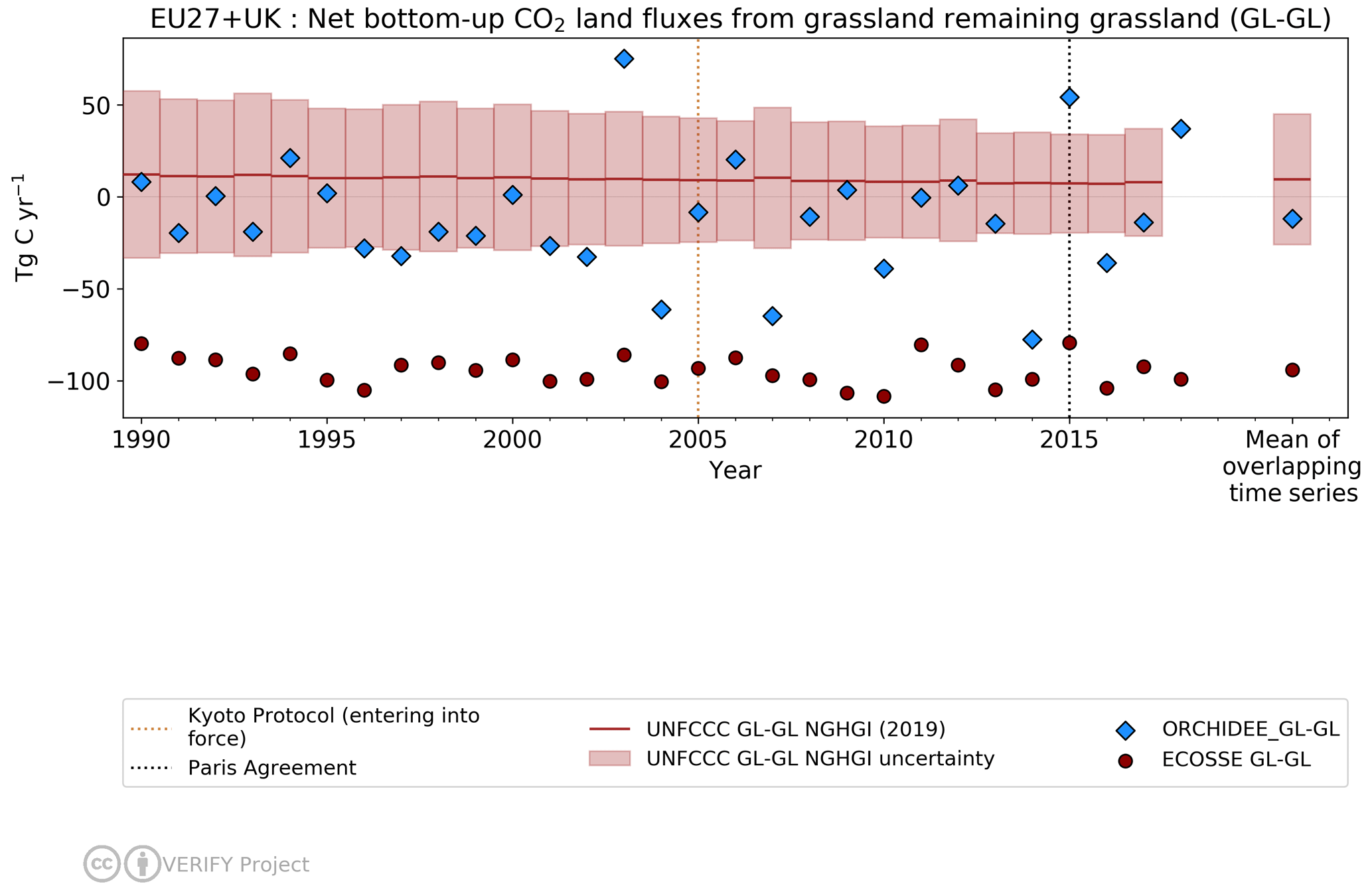
Figure 8Net CO2 flux estimates from grassland remaining grassland for the EU27 + UK CO2 from UNFCCC NGHGI (2019) submissions and bottom-up emission models with their 1990–2017 mean (on the right side). GL-GL emissions are estimated with the ORCHIDEE and ECOSSE models. The relative error on the UNFCCC value represents the UNFCCC NGHGI (2018) MS-reported uncertainty computed with the error propagation method (95 % confidence interval) and is equal to 373.6 % (no data for Hungary, Cyprus, Slovakia, Spain and the Czech Republic. The negative values represent a sink, while the positive represent a source.
For the inter-annual variability all three models follow the same dynamic, but the impacts of climate extremes are different, with significantly larger impacts in ORCHIDEE. While ORCHIDEE shows a strong reaction to drought impacts changing from a sink to a source (e.g., for 2003, which is reported as a very dry year, Ciais et al., 2005), the other two models follow ORCHIDEE's variation but show less extremes. As ECOSSE directly simulates the annual net primary production (NPP) (i.e., internal component model (MIAMI) implemented in ECOSSE) and not the intra-annual gross primary production (as in ORCHIDEE), the impact of season-specific climate anomalies is smaller than in ORCHIDEE.
Figure 8 shows the CO2 flux of the grassland remaining grassland category, GL-GL. The grassland definition in the IPCC includes rangelands and pasture land that is not considered cropland, as well as systems with vegetation that fall below the threshold used in the forest land category. This category also includes all grassland from wild lands to recreational areas as well as agricultural and silvopastoral systems, subdivided into managed and unmanaged, consistent with national definitions (Petrescu et al., 2020b). The NGHGIs of countries in the EU-27 + UK report emissions from managed pastures only, which, in 2010, represented a minimum of 58 % (Chang et al., 2016) of the total managed grassland area in the EU. Since almost all European grasslands are somehow modified by human activity and have to a major extent been created and maintained by agricultural activities, they could be defined as “semi-natural grasslands”, even if their plant communities are natural (EU LIFE, 2008). Therefore, NGHGIs report a small mean source over 1990–2017 (9 Tg C) primarily due to the use of EFs from national statistics which are linked to intensive management practices applied to grasslands in the EU.
Out of all the models used in this study, only ORCHIDEE and ECOSSE report fluxes from this category. Grasslands in ORCHIDEE do not undergo any specific management and are not separated from pasturelands. Therefore, discrepancies between ORCHIDEE and the NGHGI data result in the first reporting a mean sink over 1990–2017 of −12 Tg C while official inventories report a small source, as explained above. The sink in ORCHIDEE is due to the fact that the CO2 fertilization effect increases the NPP over time and also increases input of C to the soil, which then leads to increased soil C stocks. The strong sink simulated by ECOSSE (−94 Tg C in mean) is the result of using a limiting scenario where intensively managed grasslands, i.e., high grazing intensity and high yield removal, are not included, thus favoring high soil carbon storage. These effects are similar to that seen in croplands (see above), resulting from the CO2 fertilization effect.
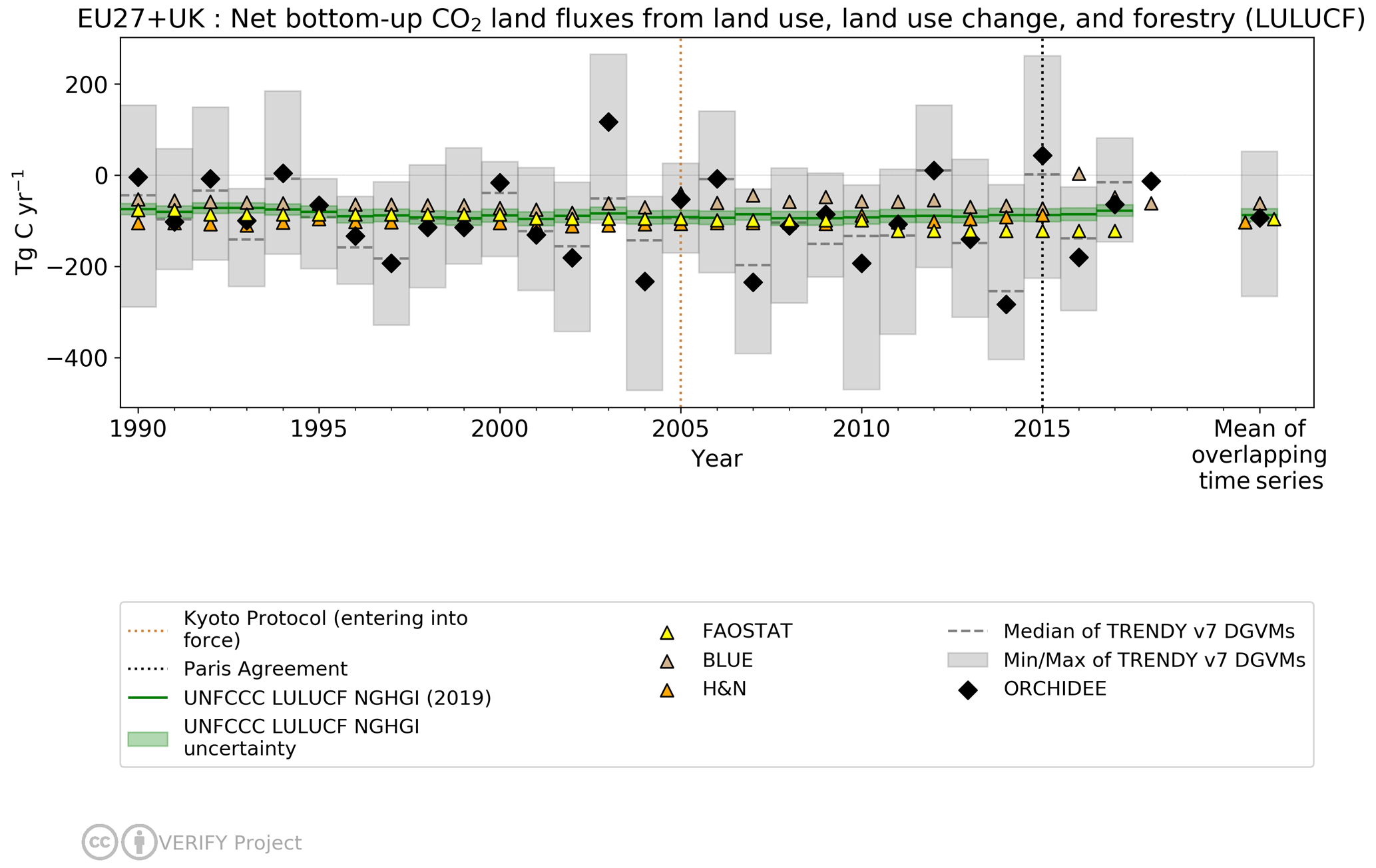
Figure 9A comparison of different estimates of the CO2 fluxes from land use, land use change and forestry activities in the EU27 + UK from seven data sources: UNFCCC NGHGI (2019), BLUE, H&N, DGVMs (TRENDY v7), FAOSTAT and ORCHIDEE (stand-alone with high-spatial-resolution forcing and from TRENDY). The grey bars represent the individual model data for eight DGVMs. The UNFCCC estimate includes the following categories: forest land, cropland, grassland, wetlands, settlements and other land from conversions, in addition to harvested wood products (HWPs). The relative error on the UNFCCC value represents the UNFCCC NGHGI (2018) MS-reported uncertainty computed with the error propagation method (95 % confidence interval) and is 16 %. The FAOSTAT estimate includes forest land, incorporating afforestation and deforestation as conversion of forest land to other land types. The means are calculated for the 1990–2015 overlapping period. The negative values represent a sink, while the positive values represent a source.
3.3.4 Bottom-up CO2 estimates from all LULUCF sectors
In this section we attempt to present a comprehensive analysis of CO2 emissions and sinks for the LULUCF sectors. Here we try to compare the sum of all categories and sectors of the NGHGIs discussed in Fig. 5 (including the remaining and transition subsectors; details are found in the Fig. 5, caption), with various observation-based BU model estimates. The comparison with atmospheric inversions (TD) is discussed in the next section. Such a comparison is challenging due to differences in terms of activities covered in the different estimates, as well as differences in terminology, which have already been highlighted in several papers (see more specifically Petrescu et al., 2020b, Fig. 12). Let's first briefly recall the main differences between the selected products.
-
FAOSTAT differs from NGHGIs for reasons summarized by Federici et al. (2015) and Petrescu et al. (2020b), including numerically different data provided by member states to FAOSTAT and UNFCCC, different methods (FAOSTAT applies a Tier 1 approach globally, while member states reports to the UNFCCC vary from Tier 1 to Tier 3), differences between net and gross land use (FAOSTAT is based on net transitions), and FAOSTAT results only considering living biomass pools instead of the five IPCC pools17 reported to the UNFCCC.
-
The process-based high-resolution ORCHIDEE simulation and the TRENDY v7 ensemble, with the so-called “S3 simulation” (see the TRENDY simulation protocol, Le Quéré et al., 2018), include the impact of CO2 fertilization, climate change and land use change for the forest, grassland and cropland sectors; they do not explicitly treat the wetland, settlement and other land sectors as in the NGHGIs. They account for the evolution of living and dead biomass as well as SOC for all categories, while for NGHGIs it is not mandatory for all subcategories (i.e., dead biomass). Finally, there is significant uncertainty associated with the DGVMs' fluxes from (i) the forcing data, including datasets of land use changes and the coverage of different land use change practices; (ii) model parameters; and (iii) structural uncertainty in models (i.e., which processes are included and which are not) (Arneth et al., 2017). Similar to FAOSTAT, DGVMs typically deal with net land use change emissions, instead of gross land use change as reported in NGHGIs, which may induce significant differences with coarse-resolution model simulations (i.e., 0.5∘ or 1∘ for the TRENDY ensemble). DGVMs often do not distinguish between managed and unmanaged land, while NGHGIs are for emissions from managed land.
-
The bookkeeping models, BLUE and H&N, calculate net emissions from land use change including immediate emissions during land conversion, legacy emissions from slash and soil carbon after land use change, regrowth of secondary forest after abandonment, and emissions from harvested wood products when they decay. They thus do not account for the net fluxes occurring in the remaining land categories due to for instance the CO2 fertilization effects or climate changes. One exception to this is fluxes from wood harvested, which is a primary source of emission on managed forest land and also included in bookkeeping models. As seen before in Fig. 5, this component can present a significant flux.
Given all these differences in terms of activities, the comparison in this section should be considered a first step that raises both important aspects of the C cycle and questions that need to be addressed in the future. Going toward a more specific comparison of only net land use change fluxes would require additional considerations. In the GCP's annual Global Carbon Budget, this term is estimated by global DGVMs as the difference between a run with and a run without land use change and by bookkeeping models. Such an estimate is given in Fig. 13 in Petrescu et al. (2020b) for forest land. While attractive, such a plot does not fully resolve the differences mentioned above. In particular, questions remain about net vs. gross land use change, managed vs. unmanaged land, and emissions from wood harvest. In addition, UNFCCC “convert” emissions (i.e., emissions resulting from land that has been converted from one type to another) are calculated for 20 years following conversion. FAOSTAT, DGVMs, and bookkeeping models typically only include convert fluxes from the year following conversion, although bookkeeping models can more easily include this transition period.
Figure 9 thus represents CO2 fluxes from LULUCF activities, including estimates from ORCHIDEE high-resolution and TRENDY (mean across the ensemble) DGVMs models (“S3” type simulations), bookkeeping models, NGHGIs and FAOSTAT. For the overlapping period 1990–2015, we observe from the means (see right part of the plot) that bookkeeping models (BLUE (−61 Tg C) and H&N (−103 Tg C)) and FAOSTAT (−96 Tg C) estimates match the UNFCCC NGHGI (−87 Tg C) reporting, because their managed areas for the EU27 + UK are similar (H&N: 118 Mha; BLUE: 117 Mha; UNFCCC: 167 Mha, from in Grassi et al., 2018a; Petrescu et al., 2020b). The unmanaged area in the EU27 + UK is negligible and sums up only 4 Mha. The similarities between bookkeeping models and UNFCCC can be explained by the fact that, despite a smaller forest sink in H&N, they both report a small sink in non-forest land uses, while for these land uses UNFCCC reports a source (Figs. 7 and 8).
The UNFCCC LULUCF estimates contain CO2 emissions from all six land use classes and HWPs, including remaining classes and conversion to and from a class to another. ORCHIDEE (−93.9 Tg C) shows large variabilities (black diamonds), mostly following the temporal patterns of the mean from TRENDY v7 DGVMs (−103 Tg C) (grey bars) as detailed above. Note again that ORCHIDEE is also part of the TRENDY ensemble but with a different meteorological forcing (coarser resolution, 0.5∘) than the one used within the VERIFY project (around 0.1∘ resolution).
The differences between bookkeeping models and UNFCCC and FAOSTAT are discussed in detail in Petrescu et al. (2020b, cf. Fig. 12), who conclude that the key difference between bookkeeping models, on the one hand, and FAOSTAT and UNFCCC methodologies, on the other, is that the latter are based on the managed land proxy (Grassi et al., 2018a). The ORCHIDEE model and the TRENDY v7 ensemble means show much higher inter-annual variability due to the sensitivity of the model fluxes to highly variable meteorological forcing and the models' sub-daily time steps, which allow for much more rapid responses to changing conditions (i.e., 2003 extreme drought year), as already discussed in the previous sections. The incorporation of variable climate data and the fact that DGVM models simulate explicitly climate impacts on CO2 fluxes, which inventories and bookkeeping do not, explain these differences.
DGVMs estimate net land use emissions as the difference between a run with and a run without land use change, and their estimate includes the loss/gain of additional sink capacity, that is, the sink that favors the environmental changes (e.g., CO2 fertilization). This sink created over forest land in the simulation without land use change is “lost” in the simulation with land use change (i.e., deforestation) because agricultural land lacks the woody material and thus has a higher carbon turnover (Gasser and Ciais, 2013; Pongratz et al., 2014, and cf. Fig. 12 in Petrescu et al., 2020b). This different definition from bookkeeping models historically implies on average higher carbon land use emissions from DGVMs when an ecosystem is converted to another with a lower carbon density, even if all post-conversion carbon stocks changes were the same in DGVMs and bookkeeping models.
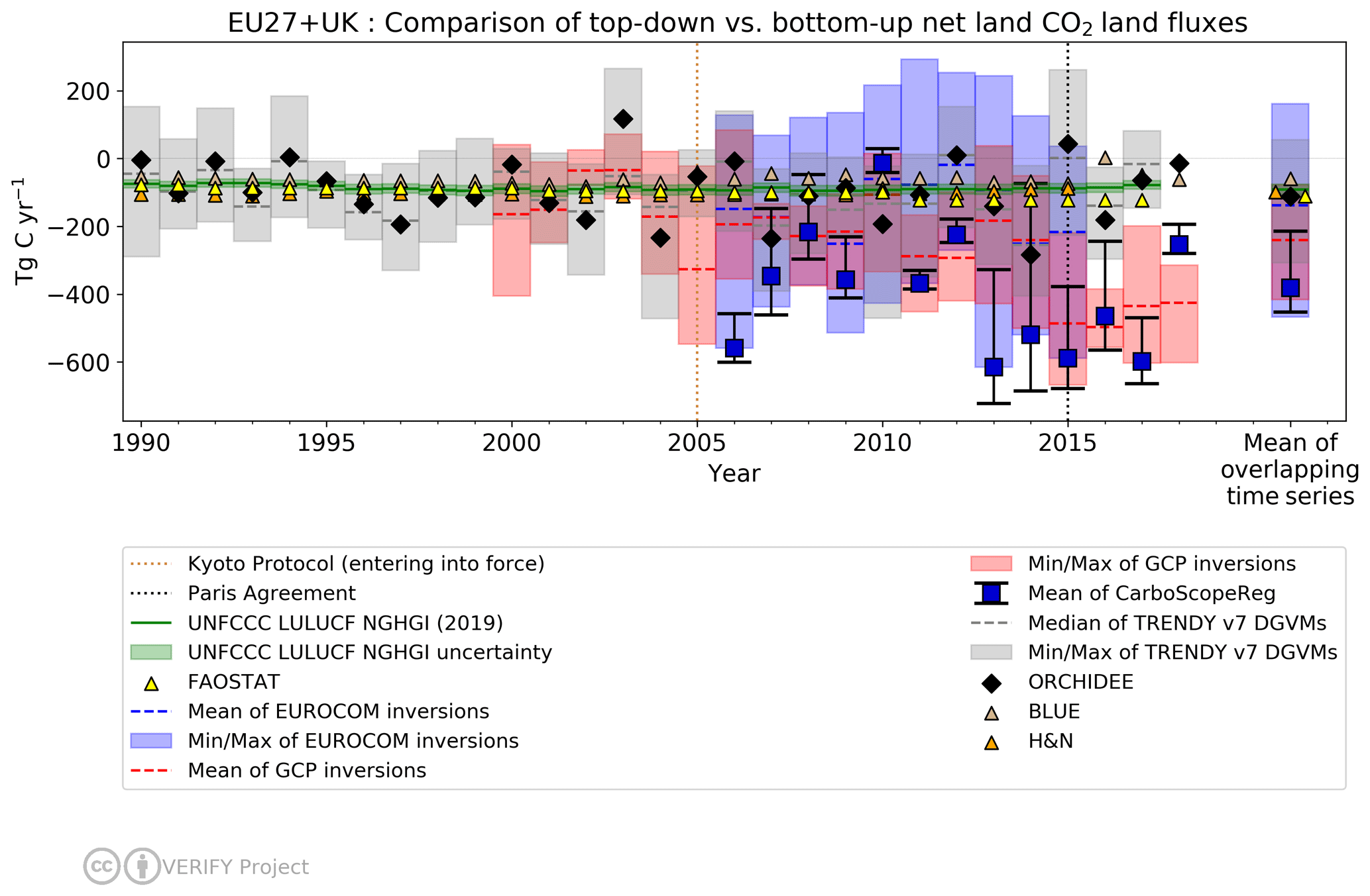
Figure 10Comparison of BU and TD total EU27 + UK biogenic CO2 estimates. The green line represents the UNFCCC NGHGI (2019). The BU estimates belong to bookkeeping models (BLUE, H&N), the grey shade is the DGVMs TRENDY v7, and we plot separately ORCHIDEE and FAOSTAT (FRA) data. The TD estimates belong to models from the ensembles GCB 2019 (red), EUROCOM (blue) and CarboScopeReg (box with whiskers). The relative error on the UNFCCC value represents the UNFCCC NGHGI (2018) MS-reported uncertainty computed with the error propagation method (95 % confidence interval) and is 16 %. The time series mean overlapping period is 2006–2015. The colored area represents the min/max of model ensemble estimates. The negative values represent a sink, while the positive represent a source. In Appendix B, Fig. B1c, we show the expanded figure of the mean time series.
3.3.5 Comparison of top-down and bottom-up CO2 estimates
Figure 10 highlights the variability of estimates from atmospheric inversions of GCP (1990–2017), CarboScopeReg (2006–2017) and EUROCOM (2006–2015) plotted against total annual EU27 + UK CO2 land emissions/removals from observation-based BU approaches and UNFCCC NGHGI (2019). In these inversions, all components of the carbon cycle (NEE) that contribute to the observed atmospheric CO2 gradients between stations (e.g., lateral fluxes, oxidation of C compounds into CO2) are included. To facilitate the comparisons with NGHGIs we first account for some of these differences by subtracting from the inversion estimates the emissions from rivers (Lauerwald et al., 2015), lakes and reservoirs (Raymond et al., 2013; Hastie et al., 2019) as NGHGIs do not include them. Also, not included in NGHGI estimates are the outgassing from crop and wood products traded and consumed this year.
Looking at TD estimates, the annual mean (overlapping period 2006–2015) of the EUROCOM inversions (−138 Tg C) is the closest inversions ensemble (among the three) to the time series mean of the NGHGI estimates (−90 Tg C), with a difference of 48 Tg C yr−1 that is well within the mean uncertainty of the regional inversion ensemble (about 250 Tg C yr−1). It also matches well with the TRENDY v7 DGVMs trend, which is smaller (+7.3 Tg C yr−2) than that of the global GCP inversions (−16 Tg C yr−1). On the other hand, the large range of variability in the EUROCOM ensemble estimates (+335 Tg C in 2015 to −615 Tg C in 2013) demonstrates that there is still a very significant uncertainty in the TD estimates. This variability seen from the TD estimates is primarily due to uncertainties in atmospheric transport modeling, boundary conditions and uncertainty inherent to the limitation of the observation network.
Additional analyses are still ongoing with the different inversion ensembles to analyze the factors controlling the large difference obtained when compared to BU approaches (for instance, the effect of the a priori fluxes, observation sites, a priori flux and observation uncertainties, and boundary conditions). This paper should be taken cautiously as a first comparison at a spatial scale not investigated so far (i.e., EU27 + UK).
The GCP results show a clear trend towards increasing the CO2 sink strength of the land surface in later years, contrary to the NGHGI estimates, which are relatively stable. Thus, the initially reasonable agreement between the two datasets (2000–2005) becomes a difference well outside the uncertainty range of the NGHGI in 2017 (290 Tg C difference between the GCP and NGHGI, with an NGHGI uncertainty of only 30 Tg C). Between 2011 and 2018, GCP (−241 Tg C mean) (red bars) shows, as well as large inter-annual variability, an increase in the CO2 sink. The strongest sink between inversions (mean −381 Tg C) is reported by CarboScopeReg, which, similar to EUROCOM, also shows high fluctuations. This fluctuation partly reflects the fact that all other inversions are results from ensembles of inversion systems each with different inter-annual variations, while CSR is a single inversion system (just a small ensemble with differing prior error structure and different set of atmospheric station data used).
Also, noteworthy is that the global inversions provide reliable results at a global scale (following the atmospheric global CO2 growth rate), but the ranges of estimates when considering continental to regional scales increase significantly due to the difficulties of the inversion systems to separate regional fluxes (e.g., Friedlingstein et al., 2020). Note also that these systems are still primarily designed for large-scale flux estimates (for instance the CarboScopeReg global system uses a transport model at coarse spatial resolution (4∘ × 5∘) and an error correlation length of 1000 km over land). The regional inversions (EUROCOM and CarboScopeReg) are still systems in development with additional complexity due to the treatment of the boundary fluxes (compared to the global systems).
For the models, differences result from choices in the simulation setup and depend on the type of model used – bookkeeping models, DGVMs or inventory-based – and whether fluxes are attributed to LULUCF emissions due to the cause or place of occurrence (indirect fluxes on managed land included in NGHGIs and FAOSTAT, e.g., changes due to human-induced climate change, including CO2 fertilization and nitrogen deposition changes) (Petrescu et al., 2020b). Table 3 below highlights these differences by presenting an overview of processes included in the models, seen for the moment as the main cause of discrepancies between estimates shown in Fig. 10.
Table 3Comparison of the processes included in the inventories, bottom-up models and inversions.
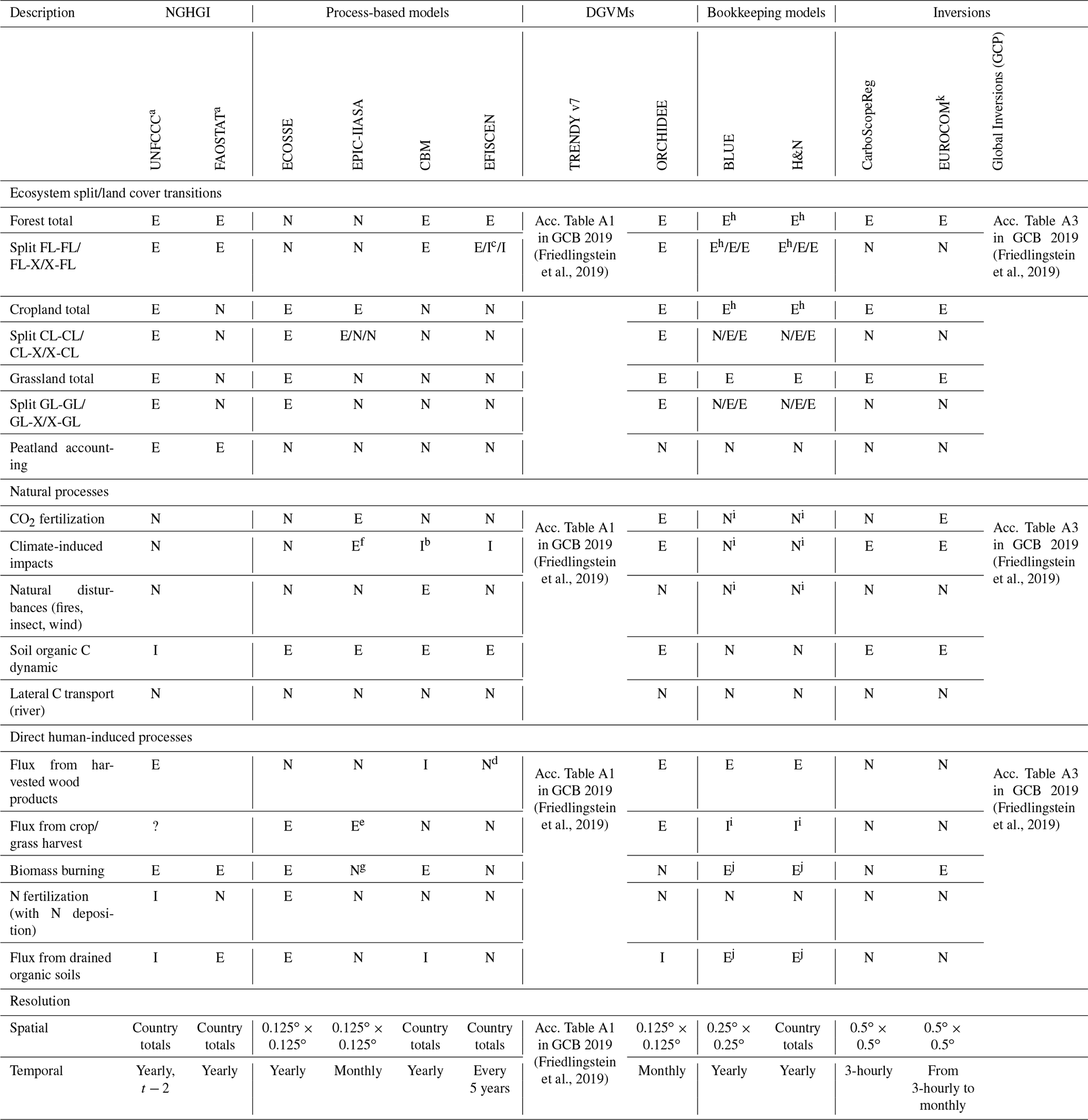
N: not included, E: explicitly modeled, I: implicitly modeled, P: partly modeled. a UNFCCC and FAOSTAT are an ensemble of country estimates calculated with specific methodology for each country, following some guidelines. b The climate effects can be estimated indirectly by CBM, using external additional input provided by other models. c EFISCEN can add this as a scenario variable; there is no internal module that allocates how much forest area there should be. d EFISCEN has only production in cubic meters but does not have a direct HWP module. e Crop yield and residue harvest from cropland (20 % of residues harvested in the case of cereals; no residue harvest for other crops). f EPIC-IIASA partly accounts for soil drought, i.e., plant growth limitation due to a lack of water in the soils. Heat stress and floods are not accounted for though. g In principle, burning of crop residues on cropland can be explicitly simulated by EPIC-IIASA. However, this is not done for VERIFY as it is not a relevant scenario for the business-as-usual cropland management in Europe. h Forest/cropland/grassland exist and have carbon stocks but have carbon fluxes only through change to management. FL-FL includes all land-use-induced effects (harvest slash and product decay, regrowth after agricultural abandonment and harvesting). i Implicit by using observation-based carbon densities that reflect harvest/climate/natural disturbances. j Peat burning and peat drainage are not bookkeeping model output but are added fromvarious data sources during post-processing. k According Table 2 in Monteil et al. (2020) and Table A3 in Friedlingstein et al. (2019).
All raw data files reported in this work which were used for calculations and figures are available for public download at https://doi.org/10.5281/zenodo.4626578 (Petrescu et al., 2020a). The data we submitted are reachable with one click (without the need for entering login and password) and downloadable with a second click, consistent with the two-click access principle for data published in ESSD (Carlson and Oda, 2018). The data and the DOI number are subject to future updates and only refers to this version of the paper.
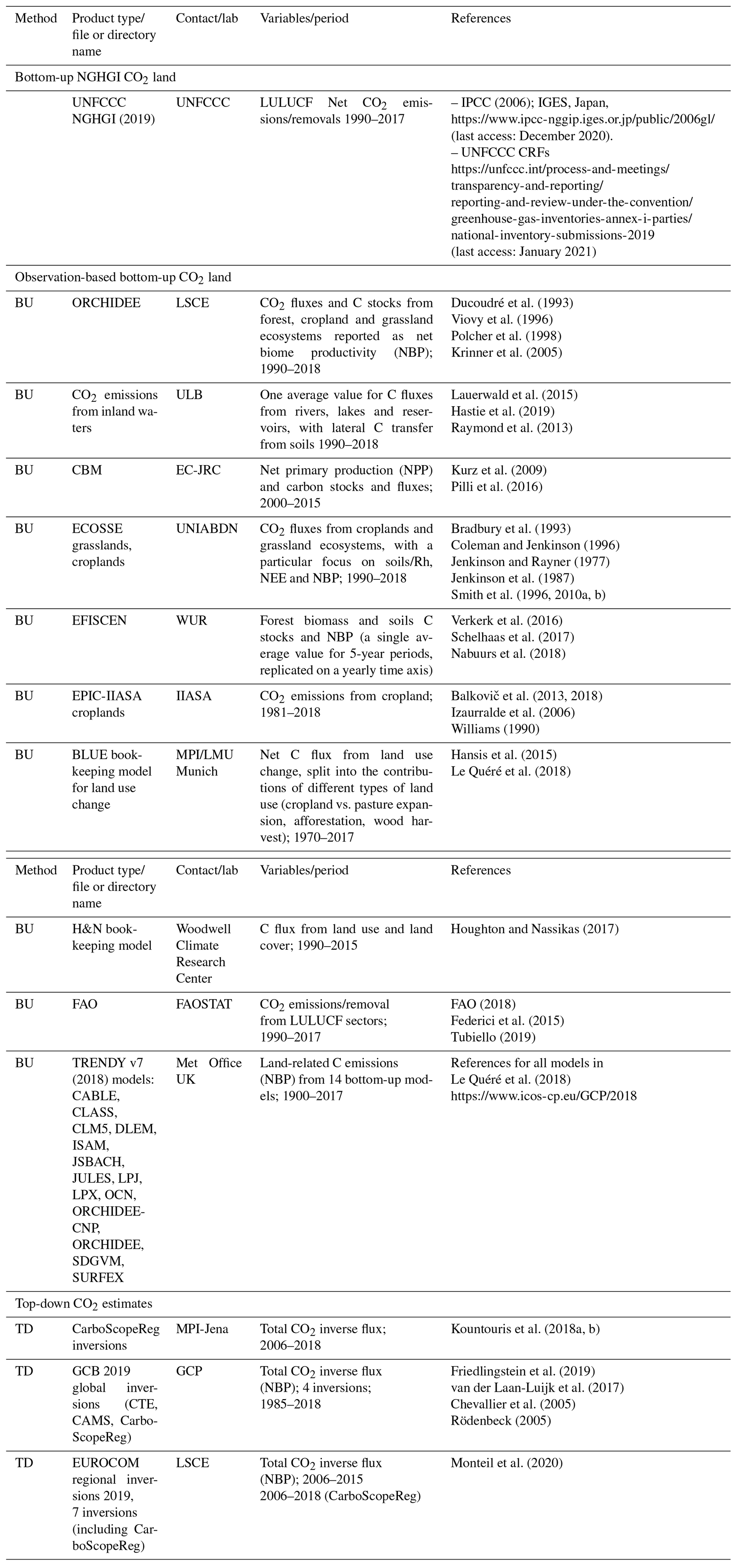
Please also see Tables 1 and 2 for an overview of data sources for CO2 emissions used in this study.
The overview and variety of data products described in this study are the first of a series of European CO2 synthesis papers presenting and investigating differences between UNFCCC NGHGIs, bottom-up data-based inventories, high-resolution observation-based BU models, and TD approaches represented by both global and regional inversions.
The CO2 fossil emissions dominate the anthropogenic CO2 flux in the EU27 + UK. Fossil CO2 emissions are more straightforward to estimate than ecosystem fluxes. Different BU methods have only minor differences with respect to the NGHGI. These differences can often be attributed to different definitions or assumptions about activity data or emission factors or by the allocation of fuel types to different sectors (see Fig. 2, Sect. 3.2). Currently, TD methods, albeit only a single inversion using CO NOx proxies to determine CO2 fossil emissions, show broad agreement with the BU estimates. The TD inversion is not yet capable of verifying the minor differences between the BU estimates. However, a substantial decrease in the level of uncertainty is expected in the near term, with the large-scale deployment of observation networks dedicated to detecting fossil fuel emissions (e.g., with the launch of the CO2M18 constellation in 2025, Maenhout al., 2020). In the short term, methodological improvements and the potential co-assimilation of existing CO2 satellite data are also expected to lead to significant decreases in the uncertainty.
The CO2 land fluxes belong to the LULUCF sector, which is one of the most uncertain sectors in UNFCCC reporting due in part to the fact that these fluxes can be either sinks or sources. The IPCC Guidelines prescribe methodologies that are used to estimate the CO2 fluxes in the NGHGI, but differences between countries continue to exist due to the use of specific national circumstances (as permitted under the 2006 IPCC Guidelines). When we analyzed the estimates from multiple BU sources (inventories and models), we observe similar sources of uncertainties: (a) differences due to input data and structural/parametric uncertainty of models (Houghton et al., 2012) and (b) differences in definitions (Pongratz et al., 2014; Grassi et al., 2018b; Petrescu et al., 2020b). More accurate estimates for LULUCF data will be needed in the post-2020 reporting for the EU27 and UK since the LULUCF sector will now contribute to the EU's 2030 targets. To better assess natural variability and trends we believe a reconciliation of BU and TD estimates should focus on clearly defined activities over a given period (e.g., 5 years) and regions as presented in Fig. 4. The considerable differences in the agreement between BU and TD estimates from regional split are related to areas and for some regions (e.g., eastern Europe) sparseness of observation data. Regarding the detailed sector-specific and inversion results (Figs. 6–10), often differences come from choices in the simulation setup and depend on the type of model used – bookkeeping models, DGVMs, inventory-based or inversion ensembles. Results also differ based on whether fluxes are attributed to LULUCF emissions due to the cause (e.g., direct or indirect) or place of occurrence. For example, indirect fluxes on managed land are included in NGHGIs and FAOSTAT, while additional sink capacity (e.g., Petrescu et al, 2020b) is included in estimates from process-based models (e.g., ORCHIDEE or TRENDY DGVMs). A more in depth analysis of the regional/country level is foreseen as part of the overall long-term objectives of VERIFY.
All observation-based BU estimates for LULUCF presented in this study show similar magnitudes and trends compared to the NGHGIs but generally differ in the specific values. We notice stronger similarities between NGHGIs and models using national forest inventory data (e,g. CBM, EFISCEN). For cropland and grassland sector-specific models (ECOSSE, EPIC-IIASA) the differences between their results and the NGHGIs are due to differences in input data, process representation (in particular those linked to soil organic matter decomposition) and management representation. In general, management is one of the main drivers for the carbon balance of croplands and grasslands. However, spatial data on management are scarce and can have high uncertainty. For EPIC-IIASA specifically, the regional carbon simulation results for managed cropland are almost evenly impacted by model parameterization, soil input accuracy and crop management regionalization (Balkovič et al., 2020). For the overall estimation of emissions from LULUCF activities on all land types (Fig. 9), the comparison is made more challenging as results from both land use and land use changes are presented. Comparing only the effect of land use change (conversion) is non-trivial and presents an area for improvement to be handled in next synthesis.
Observation-based BU estimates of LULUCF provide large year-to-year flux variability (Figs. 6–9), contrary to the NGHGIs, primarily due to the effect of varying meteorology especially through the duration and intensity of the summer growing season, which can vary significantly between years (Bastos et al., 2020; Thompson et al., 2020). In the framework of periodic NGHGI assessments, the choice of a reference period (usually 5 years, or a biannual reporting) may be critical in the context of large flux inter-annual variability. One direction could be to include in the NGHGIs EFs derived from the observation-based approaches (both BU and TD) in the form of year-to-year flux anomalies. The TD inversion estimates also show pronounced inter-annual variability results (Figs. 10 and B1c for mean values). Uncertainties in the inversion results are primarily due to uncertainties in atmospheric transport modeling, boundary conditions and uncertainty inherent to the limitation of the observation network. Currently, regional inversions (CarboScopeReg and EUROCOM) are still systems under development which face different challenges from the much-coarser-resolution global systems used here to represent regional results (GCP ensemble including CarboScopeReg global).
The next steps needed to improve and facilitate the reconciliation between BU and TD estimates will include (1) as already discussed in Petrescu et al. (2020b), BU process-based models incorporating unified protocols and guidelines for uniform definitions which should be able to disaggregate their estimates to facilitate comparison to NGHGIs and 2006 IPCC practices (i.e., managed vs. unmanaged land, 20-year legacy for classes remaining in the same class, distinction of fluxes arising solely from land use change); (2) for sector-specific models, especially for cropland and grassland, improving treatment of the contribution of the soil organic carbon dynamic to the budget; (3) for TD estimates, the use of the Community Inversion Framework currently under development (Berchet et al., 2020) to better assess the different sources of uncertainties from the inversion setups (model transport, prior fluxes, observation networks); (4) for the overall comparison of BU and TD fluxes, the incorporation of the contribution of lateral fluxes of carbon by human activities and rivers that connect CO2 uptake in one area with its release in another (Ciais et al., 2020).
From this analysis we demonstrate that a complete, ready-for-purpose monitoring system providing annual carbon fluxes across Europe does not yet exist. Therefore, for consistent future estimates to be used in the global stocktake exercise to reach the Paris Agreement targets, significant effort must still be undertaken to reduce the uncertainty across all potential methods used in such a system (e.g., Janssens-Maenhout et al., 2020).
The country-specific plots are found at http://webportals.ipsl.jussieu.fr/VERIFY/FactSheets/ (upon registration, last access: February 2021) (v1.24).
VERIFY project
VERIFY's primary aim is to develop scientifically robust methods to assess the accuracy and potential biases in national inventories reported by the parties through an independent pre-operational framework. The main concept is to provide observation-based estimates of anthropogenic and natural GHG emissions and sinks as well as associated uncertainties. The proposed approach is based on the integration of atmospheric measurements, improved emission inventories, ecosystem data, and satellite observations, as well as on an understanding of processes controlling GHG fluxes (ecosystem models, GHG emission models).
Two complementary approaches relying on observational data streams will be combined in VERIFY to quantify GHG fluxes:
-
atmospheric GHG concentrations from satellites and ground-based networks (top-down atmospheric inversion models) and
-
bottom-up activity data (e.g., fuel use and emission factors) and ecosystem measurements (bottom-up models).
For CO2, a specific effort will be made to separate fossil fuel emissions from ecosystems fluxes. For CH4 and N2O, we will separate agricultural from fossil fuel and industrial emissions. Finally, trends in the budget of the three GHGs will be analyzed in the context of NDC targets.
The objectives of VERIFY are as follows.
-
Objective 1. Integrate the efforts between the research community, national inventory compilers, operational centers in Europe and international organizations towards the definition of future international standards for the verification of GHG emissions and sinks based on independent observation.
-
Objective 2. Enhance the current observation and modeling ability to accurately and transparently quantify the sinks and sources of GHGs in the land use sector for the tracking of land-based mitigation activities.
-
Objective 3. Develop new research approaches to monitor anthropogenic GHG emissions in support of the EU commitment to reduce GHG emissions by 40 % by 2030 compared to the year 1990.
-
Objective 4. Produce periodic scientific syntheses of an observation-based GHG balance of EU countries and practical policy-oriented assessments of GHG emission trends and apply these methodologies to other countries.
For more information on project team and products/results check https://verify.lsce.ipsl.fr/ (last access: November 2020).
Table A1Country grouping used for comparison purposes between BU and TD emissions. Countries highlighted in italic are not discussed in the current 2019 synthesis mostly because of unavailability of UNFCCC NGHGI reports (non-Annex I countries*) but are present on the following web portal: http://webportals.ipsl.jussieu.fr/VERIFY/FactSheets/ (last access: February 2021). Results of Annex I countries (NOR, CHE, ISL) and non-EU eastern European countries (EAE) are represented in Fig. 4.
* Non-Annex I countries are mostly developing countries. The reporting to UNFCCC is implemented through national communications (NCs) and biennial update reports (BURs): https://unfccc.int/national-reports-from-non-annex-i-parties(last access: November 2020).
Table A2Main methodological changes of the current study with respect to Petrescu et al. (2020b). The sectors are highlighted in italics; the changes with respect to AFOLU (Petrescu et al., 2020a) are shown in bold. “NA” means that there are no data available.
A1 Fossil CO2 emissions
A1.1 Bottom-up emission estimates
For further details, see Andrew (2020).
UNFCCC NGHGI (2019)
The Annex I Parties to the UNFCCC are required to report emissions inventories annually using the common reporting format (CRF). This annual published dataset includes all CO2 emissions sources for those countries and for most countries for the period 1990 to t−2. Some eastern European countries' submissions begin in the 1980s. Revisions are made on an irregular basis outside of the standard annual schedule. For a complete description see Andrew (2020).
Uncertainties. Annex I Parties quantitatively estimate their uncertainties of data used for all source and sink categories using the methodologies provided in the 2006 IPCC Guidelines. The 2006 IPCC Guidelines stipulate that the determination of uncertainties is a key element of any complete inventory. Uncertainties are quantified for emission factors, activity data and, in some cases, for emissions. In general, two methods for determining uncertainties are differentiated. The Tier 1 method combines, in a simple way, the uncertainties in activity data and emission factors for each category and greenhouse gas and then aggregates these uncertainties for all categories and greenhouse gas components to obtain the total uncertainty for the inventory. The Tier 2 method for uncertainty determination is the same in principle, but it also considers the distribution function for uncertainties and carries out aggregation using Monte Carlo simulation. In the Tier 2 method, the process also necessarily includes the determination of the probability density function for both parameters.
EDGAR v5.0
The first edition of the Emissions Database for Global Atmospheric Research was published in 1995. The dataset now includes almost all sources of fossil CO2 emissions, is updated annually and reports data for 1970 to n−1. Estimates are provided by sector. Emissions are estimated fully based on statistical data from 1970 until 2015, while for the years beyond 2015 a fast-track (FT) approach is applied based on BP data and other proxies to extrapolate CO2 emissions until most recent years (Crippa et al., 2019, https://edgar.jrc.ec.europa.eu/overview.php?v=booklet2019, last access: 14 April 2020). For a complete description see Andrew (2020).
Uncertainties. EDGAR uses emission factors (EFs) and activity data (AD) to estimate emissions. Both EFs and AD are uncertain to some degree, and when combined, their uncertainties need to be combined too. To estimate EDGAR's uncertainties (stemming from a lack of knowledge of the true value of the EFs and AD), the methodology devised by IPCC (2006, chap. 3) is adopted, that is, the sum of squares of the uncertainty of the EFs and AD (uncertainty of the product of two variables). A lognormal probability distribution function is assumed to avoid negative values, and uncertainties are reported as a 95 % confidence interval according to IPCC (2006, chap. 3, Eq. 3.7). For emission uncertainties in the range 50 % to 230 %, a correction factor is adopted as suggested by Frey et al. (2003) and IPCC (2006, chap. 3, Eq. 3.4).
BP
BP releases its Statistical Review of World Energy annually in June, with the first report being published in 1952. Primarily an energy dataset, BP also includes estimates of fossil fuel CO2 emissions derived from its energy data. The emission estimates are totals for each country starting in 1965 to year n−1. For a complete description see Andrew (2020).
CDIAC
The original Carbon Dioxide Information Analysis Center included a fossil CO2 emissions dataset that was long known as CDIAC. This dataset is now produced at Appalachian State University and includes emissions from fossil fuels and cement production from 1751 to n−3. Fossil fuel emissions are derived from UN energy statistics and cement emissions from USGS production data. For a complete description see Andrew (2020).
EIA
The US Energy Information Administration publishes international energy statistics and from these derives estimates of energy combustion CO2 emissions. Data are currently available for the period 1980–2016. For a complete description see Andrew (2020).
IEA
The International Energy Agency publishes international energy statistics and from these derives estimates of energy combustion CO2 emissions including from the use of coal in the iron and steel industry. Emission estimates start in 1960 for OECD members and 1971 for non-members and run through n−1 for OECD members' totals and n−2 for members' details and non-members. Estimates are available by sector for a fee. For a complete description see Andrew (2020).
GCP
The Global Carbon Project includes estimates of fossil CO2 emissions in its annual Global Carbon Budget publication. These includes emissions from fossil fuels and cement production for the period 1750 to n−1. For a complete description see Andrew (2020).
CEDS
The Community Emissions Data System has included estimates of fossil CO2 emissions since 2018, with an irregular update cycle. Energy data are directly from IEA, but emissions are scaled to higher-priority sources, including national inventories. Almost all emissions sources are included, and estimates are published for the period 1750–2014. Estimates are provided by sector. For a complete description see Andrew (2020).
A1.2 Top-down CO2 emission estimates
Fast-track fossil CO2 emission inversion
The so called KL18 inversion product (Konovalov and Lvova, 2018) consists in a rescaling of the 0.1∘ × 0.1∘ resolution maps of annual averages of fossil CO2 anthropogenic emissions in western Europe (over 11 countries of the European Union – Portugal, Spain, France, Belgium, Luxembourg, Netherlands, UK, Germany, Denmark, Italy and Austria – and Switzerland) from the EDGARv4.3.2 inventory (Janssens-Maenhout et al., 2019). It has been produced by IAP-RAS to provide first inversions of the emissions in Europe during the first years of VERIFY, while the development of the main inversion system for this task should last more than 2 years. It covers the years 2012 to 2015, updating the method and extending the inversions documented in Konovalov et al. (2016). The factors scaling the EDGARv4.3.2 maps are derived from the regional inversions of CO and NOx emissions from the European Monitoring and Evaluation Programme (EMEP) Centre on Emission Inventories and Projections (CEIP) as prior knowledge of the emissions and CO2 CO and CO2 NOx emission ratios associated with the combustion of fossil from EDGARv4.3.2. These regional inversions are based on the assimilation of satellite atmospheric concentration data: total column CO from IASI and tropospheric column NO2 from OMI in a 50 km resolution European configuration of the CHIMERE mesoscale atmospheric chemistry–transport model (Menut et al., 2013). The resulting fCO2 inverse emissions are calculated by converting the inverted CO and NOx emission (sectoral or total) budgets into fCO2 emissions budgets using ratios of CO (all emissions) fCO2 (fossil fuel missions only) and NOx (all emissions) fCO2 (fossil fuel emissions only) from EDGAR (excluding biofuel from the CO2 emissions in EDGAR but not from the CO and NOx emissions in EDGAR).
Uncertainty. An estimate of the uncertainty in the annual budgets of the emissions over the 12 countries is derived from the analyses of uncertainties within the CO and NOx emission inversions (associated with model and data errors) and from an assessment of the uncertainties in the CO2 CO and CO2 NOx emission ratios (based on their spatial variability). The preliminary results indicate that the uncertainty in the information from the CO inversion is too high to provide reliable estimates of the CO2 fossil emissions when using CO satellite data only or to provide weight to this information when using CO2 fossil estimates from both the CO and NOx inversions. The estimates based on NO2 data are close to EDGAR v4.3.2 in 2012. These estimates are quite constant over the 4-year period, while we assume that the CO2 fossil emissions followed a significant negative trend during this period. The analysis shows that the uncertainties in these estimates can explain the difficulty to detect such a trend.
A2 Land CO2 emissions/removals
A2.1 Bottom-up CO2 estimates
UNFCCC NGHGI 2019 – LULUCF
Under the convention and its Kyoto Protocol, national greenhouse gas (GHG) inventories are the most important source of information to track progress and assess climate protection measures by countries. In order to build mutual trust in the reliability of GHG emission information provided, national GHG inventories are subject to standardized reporting requirements, which have been continuously developed by the Conference of the Parties (COP)19. The calculation methods for the estimation of greenhouse gases in the respective sectors are determined by the methods provided by the 2006 IPCC Guidelines for National Greenhouse Gas Inventories (IPCC, 2006). They provide detailed methodological descriptions to estimate emissions and removals, as well as provide recommendations to collect the activity data needed. As a general overall requirement, the UNFCCC reporting guidelines stipulate that reporting under the convention and the Kyoto Protocol must follow the five key principles of transparency, accuracy, completeness, consistency and comparability (TACCC). The reporting under UNFCCC shall meet the TACCC principles. The three main GHGs are reported in time series from 1990 up to 2 years before the due date of the reporting. The reporting is strictly source category based and is done under the common reporting format tables (CRFs), downloadable from the UNFCCC official submission portal: https://unfccc.int/process-and-meetings/transparency-and-reporting/reporting-and-review-under-the-convention/greenhouse-gas-inventories-annex-i-parties/national-inventory-submissions-2019 (last access: January 2021).
For the biogenic CO2 emissions from sector 4 LULUCF, methods for the estimation of CO2 emissions and removals differ enormously among countries and land use categories. Each country uses its own country-specific method, which takes into account specific national circumstances (as long as they are in accordance with the 2006 IPCC Guidelines), as well as IPCC default values, which are usually more conservative and result in higher uncertainties. The EU GHG inventory underlies the assumption that the individual use of national country-specific methods leads to more accurate GHG estimates than the implementation of a single EU wide approach (UNFCCC, 2018). Key categories for the EU28 are 4.A.1. and 4.A.2. – forest land remaining forest land and land converted to forest land; 4.B.1. and 4.B.2. – cropland remaining cropland and land converted to cropland; 4.C.1. and 4.C.2. – grassland remaining grassland and land converted to grassland; 4.D.1. and 4.D.2. – wetlands remaining wetlands and land converted to wetlands; 4.E.1. and 4.E.2. – settlements remaining settlements and land converted to settlements; and 4.G – harvested wood products (HWPs). The tier method a country applies depends on the national circumstances and the individual conditions of the land, which explains the variability of uncertainties among the sector itself as well as among EU countries.
The uncertainty methodology for the NGHGI UNFCCC submissions is based on chap. 3 of 2006 IPCC Guidelines for National Greenhouse Gas Inventories and is the same as in Sect. 2.1 and Petrescu et al. (2020b, Appendix B).
ORCHIDEE
ORCHIDEE is a general ecosystem model designed to be coupled to an atmospheric model in the context of modeling the entire Earth system. As such, ORCHIDEE calculates its prognostic variables (i.e., a multitude of C, H2O and energy fluxes) from the following environmental drivers: air temperature, wind speed, solar radiation, air humidity, precipitation and atmospheric CO2 concentration. As the run progresses, vegetation grows on each pixel, divided into 13 generic types (e.g., broadleaf temperate forests, C3 crops), which cycle carbon between the soil, land surface, and atmosphere through processes such as photosynthesis, litter fall and decay. Limited human activities are included through the form of generic wood and crop harvests, which remove aboveground biomass on an annual basis.
Among other environmental indicators, ORCHIDEE simulates positive and negative CO2 emissions from plant uptake, soil decomposition and harvests across forests, grasslands and croplands. Activity data are based on land use and land cover maps. For VERIFY, pixel land cover/land use fractions were based on the land use map LUH2v2h and the land cover project of the Climate Change Initiative (CCI) program of the European Space Agency (ESA). The latter is based on purely remotely sensed methods, while the former makes use of national harvest data from the UN Food and Agriculture Organization.
ESA-CCI LUH2v2. “We describe here the input data and algorithms used to create the land cover maps specific for our CMIP6 simulations using the historical/future reconstruction of land use states provided as reference datasets for CMIP6 within the land use harmonization database LUH2v2h (Hurtt et al., 2020). More details are provided on the devoted web page https://orchidas.lsce.ipsl.fr/dev/lccci (last access: October 2020) which shows further tabular, graphical and statistical data. The overall approach relies on the combination of the LUH2v2 data with present-day land cover distribution derived from satellite observations for the past decades. The main task consists in allocating the land use types from LUH2v2 in the different PFTs for the historical period and the future scenarios. The natural vegetation in each grid cell is defined as the PFT distribution derived from the ESA-CCI land cover product for the year 2010 to which pasture fraction and crop fraction from LUH2v2 (for the year 2010) have been subtracted from grass and crop PFTs. This characterization of the natural vegetation in terms of PFT distribution is assumed invariant in time and is used for both the historical period and the different future scenarios.” (Lurton et al., 2020).
Uncertainty in the ORCHIDEE model arises from three primary sources: parameters, forcing data (including spatial and temporal resolution) and model structure. Some researchers argue that the initial state of the model (i.e., the values of the various carbon and water pools at the beginning of the production run, following model spinup) represents a fourth area. However, the initial state of the model is defined by its equilibrium state and therefore a strong function of the parameters, forcing data and model structure, with the only independent choice being the target year of the initial state. Out of the three primarily areas of uncertainty, the climate forcing data are dictated by the VERIFY project itself, thus removing that source from explaining observed differences among the models, although it can still contribute to uncertainty between the ORCHIDEE results and the national inventories. The land use/land cover maps, another major source of uncertainty for ORCHIDEE carbon fluxes, have also been harmonized to a large extent between the bottom-up carbon budget models in the project. Parameter uncertainty and model structure thus represent the two largest sources of potential disagreement between ORCHIDEE and the other bottom-up carbon budget models. Computational cost prevents a full characterization of uncertainty due to parameter selection in ORCHIDEE (and dynamic global vegetation models in general), and uncertainties in model structure require the use of multiple models of the same type but including different physical processes. Such a comparison has not been done in the context of VERIFY, although the results from the TRENDY suite of models shown in the figures (Figs. 9 and 10) give a good indication of this.
CO2 emissions from inland waters
These estimates represent a climatology of average annual CO2 emissions from rivers, lakes and reservoirs at the spatial resolution of 0.1∘. The approach combines CO2 evasion fluxes from the global river network, as estimated by the empirical model of Lauerwald et al. (2015) with the lake and reservoir estimates by Hastie et al. (2019) for the boreal biome and by Raymond et al. (2013) for the lower latitudes. The Lauerwald et al. (2015) and Hastie et al. (2019) studies follow the same approach and rely on the development of a statistical prediction model for inland water pCO2 at 0.5∘ using global, high-resolution geodata. The pCO2 climatology was then combined with different estimates of the gas transfer velocity k to produce the resulting map of CO2 evasion. The Raymond et al. (2013) study only provides mean flux densities at the much coarser spatial resolution of the so-called COSCAT regions. All estimates were then downscaled to 0.1∘ using the spatial distribution of European inland water bodies. Note that in contrast to Hastie et al. (2019) the areal distribution of lakes was extracted from the HydroLAKES database (Messager et al., 2016) to be consistent with the estimates of inland water N2O and CH4 presented by Petrescu et al. (2021).
Uncertainty. Monte Carlo simulations were performed to constrain uncertainties resulting from both the pCO2 prediction equation and the choice of the k formulation.
CBM
The Carbon Budget Model developed by the Canadian Forest Service (CBM-CFS3) can simulate the historical and future stand- and landscape-level C dynamics under different scenarios of harvest and natural disturbances (fires, storms), according to the standards described by the IPCC (Kurz et al., 2009). Since 2009, the CBM has been tested and validated by the Joint Research Centre of the European Commission (JRC) and adapted to the European forests. It is currently applied to 26 EU member states, both at the country and NUTS2 level (Pilli et al., 2016).
Based on the model framework, each stand is described by area, age and land use classes and up to 10 classifiers based on administrative and ecological information and on silvicultural parameters (such as forest composition and management strategy). A set of yield tables define the merchantable volume production for each species, while species-specific allometric equations convert merchantable volume production into aboveground biomass at the stand level. At the end of each year the model provides data on the net primary production (NPP), carbon stocks and fluxes, as the annual C transfers between pools and to the forest product sector.
The model can support policy anticipation, formulation and evaluation under the LULUCF sector, and it is used to estimate the current and future forest C dynamics, both as a verification tool (i.e., to compare the results with the estimates provided by other models) and to support the EU legislation on the LULUCF sector (Grassi et al., 2018a). In the biomass sector, the CBM can be used in combination with other models to estimate the maximum wood potential and the forest C dynamic under different assumptions of harvest and land use change (Jonsson et al., 2018).
Uncertainty. Quantifying the overall uncertainty of CBM estimates is challenging because of the complexity of each parameter. The uncertainty in CBM arises from three primary sources: parameters, forcing data (including spatial and temporal resolution) and model structure. It is linked to both activity data and emission factors (area, biomass volume implied by the species-specific equation to convert the merchantable volume to total aboveground biomass (used as a biomass expansion factor)) as well to the capacity of each model to represent the original values, in this case estimated through the mean percentage difference between the predicted and observed values. A detailed description of the uncertainty methodology is found in Pilli et al. (2017).
EFISCEN
The European Forest Information SCENario Model (EFISCEN) is a large-scale forest model that projects forest resource development on the regional to European scale. The model uses national forest inventory data as a main source of input to describe the current structure and composition of European forest resources. The model projects the development of forest resources, based on scenarios for policy, management strategies and climate change impacts. With the help of biomass expansion factors, stem wood volume is converted into whole-tree biomass and subsequently to whole-tree carbon stocks. Information on litter fall rates, felling residues and natural mortality is used as input into the soil module YASSO (Liski et al., 2005), which is dynamically linked to EFISCEN and delivers information on forest soil carbon stocks. The core of the EFISCEN model was developed by Ola Sallnäs at the Swedish Agricultural University (Sallnäs, 1990). It has been applied to European countries in many studies since then, dealing with a diversity of forest resource and policy aspects. A detailed model description is given by Verkerk et al. (2016), with online information on the availability and documentation of EFISCEN at http://efiscen.efi.int (last access: October 2020). The model and its source code are freely available, distributed under the GNU General Public License conditions (http://www.gnu.org/licenses/gpl-3.0.html, last access: October 2020).
Uncertainties. The sensitivity analysis on EFISCEN v3 is described in detail by Schelhaas et al. (2007) (the manual). Total sensitivity is mostly caused by young forest growth, width of volume classes and age of felling.
EPIC-IIASA (croplands)
The Environmental Policy Integrated Climate (EPIC) model is a field-scale process-based model (Izaurralde et al., 2006; Williams, 1990) which calculates, with a daily time step, crop growth and yield, hydrological, nutrient and carbon cycling, soil temperature and moisture, soil erosion, tillage, and plant environment control. Potential crop biomass is calculated from photosynthetically active radiation using the radiation-use-efficiency concept modified for vapor pressure deficit and atmospheric CO2 concentration effect. Potential biomass is adjusted to actual biomass through daily stress caused by extreme temperatures, water and nutrient deficiency, or inadequate aeration. The coupled organic C and N module in EPIC (Izaurralde et al., 2006) distributes organic C and N between three pools of soil organic matter (active, slow and passive) and two litter compartments (metabolic and structural). EPIC calculates potential transformations of the five compartments as regulated by soil moisture, temperature, oxygen, tillage and lignin content. Daily potential transformations are adjusted to actual transformations when the combined N demand in all receiving compartments exceeds the N supply from the soil. The transformed components are partitioned into CO2 (heterotrophic respiration), dissolved C in leaching (DOC) and the receiving SOC pools. EPIC also calculates SOC loss with erosion.
The EPIC-IIASA (version EU) modeling platform was built by coupling the field-scale EPIC version 0810 with large-scale data on land cover (cropland), soils, topography, field size and crop management practices aggregated at a 1 × 1 km grid covering European countries (Balkovič et al., 2018, 2013). In VERIFY, a total of 10 major European crops including winter wheat, winter rye, spring barley, grain maize, winter rapeseed, sunflower, sugar beet, potatoes, soybean and rice were used to represent agricultural production systems in Europe. Crop fertilization and irrigation were estimated for NUTS2 statistical regions between 1995 and 2010 (Balkovič et al., 2013). For VERIFY, the simulations were carried out assuming conventional tillage, consisting of two cultivation operations and mouldboard ploughing prior to sowing and an offset disking after harvesting of cereals. Two row cultivations during the growing season were simulated for maize and one ridging operation for potatoes. It was assumed that 20 % of crop residues are removed in the case of cereals (excluding maize), while no residues are harvested for other crops.
Uncertainties in EPIC arise from three primary sources which were described in detail by ORCHIDEE. A detailed sensitivity and uncertainty analysis of EPIC-IIASA regional carbon modeling is presented in Balkovič et al. (2020).
ECOSSE (grasslands)
ECOSSE is a biogeochemical model that is based on the carbon model RothC (Jenkinson and Rayner, 1977; Jenkinson et al., 1987; Coleman and Jenkinson, 1996) and the nitrogen model SUNDIAL (Bradbury et al., 1993; Smith et al., 1996). All processes of the carbon and nitrogen dynamics are considered (Smith et al., 2010a, b). Additionally, in ECOSSE processes of minor relevance for mineral arable soils are implemented as well (e.g., methane emissions) to have a better representation of processes that are relevant for other soils (e.g., organic soils). ECOSSE can run in different modes and for different time steps. The two main modes are site-specific and limited data. In the later version, basis assumptions/estimates for parameters can be provided by the model. This increases the uncertainty but makes ECOSSE a universal tool that can be applied for large-scale simulations even if the data availability is limited. To increase the accuracy in the site-specific version of the model, detailed information about soil properties, plant input, nutrient application and management can be added as available.
During the decomposition process, material is exchanged between the soil organic matter (SOM) pools according to first-order rate equations; characterized by a specific rate constant for each pool; and modified according to rate modifiers dependent on the temperature, moisture, crop cover and pH of the soil. The model includes five pools with one of them inert. The N content of the soil follows the decomposition of the SOM, with a stable C : N ratio defined for each pool at a given pH and with N being either mineralized or immobilized to maintain that ratio. Nitrogen released from decomposing SOM as ammonium (NH) or added to the soil may be nitrified to nitrate (NO).
For spatial simulations the model is implemented in a spatial model platform. This allows us to aggregate the input parameter for the needed resolution. ECOSSE is a one-dimensional model and the model platform provides the input data in a spatial distribution and aggregates the model outputs for further analysis. While climate data are interpolated, soil data are represented by the dominant soil type or by the proportional representation of the different soil types in the spatial simulation unit (this is a grid cell in VERIFY).
Uncertainties in ECOSSE arise from three primary sources: parameters, forcing data (including spatial and temporal resolution) and model structure. These uncertainties are not yet quantified.
Bookkeeping models
We make use of data from two bookkeeping models: BLUE (Hansis et al., 2015) and H&N (Houghton and Nassikas, 2017).
The BLUE model provides a data-driven estimate of the net land use change fluxes. BLUE stands for “bookkeeping of land use emissions”. Bookkeeping models (Hansis et al., 2015; Houghton et al., 1983) calculate land use change CO2 emissions (sources and sinks) for transitions between various natural vegetation types and agricultural lands. The bookkeeping approaches keep track of the carbon stored in vegetation, soils and products before and after the land use change. In BLUE, land use forcing is taken from the land use harmonization, LUH2, project for estimates within the annual Global Carbon Budget. The model provides data at annual time steps and 0.25∘ resolution. Temporal evolution of carbon gain or loss, i.e., how fast carbon pools decay or regrow following a land use change, is based on response curves derived from literature. The response curves describe decay of vegetation and soil carbon, including transfer to product pools of different lifetimes, as well as carbon uptake due to regrowth of vegetation and subsequent refilling of soil carbon pools.
The H&N model (Houghton, 1983) calculates land use change CO2 emissions and uptake fluxes for transitions between various natural vegetation types and agricultural lands (croplands and pastures). The original bookkeeping approach of Houghton (2003) keeps track of the carbon stored in vegetation and soils before and after the land use change. Carbon gain or loss is based on response curves derived from literature. The response curves describe decay of vegetation and soil carbon, including transfer to product pools of different lifetimes, as well as carbon uptake due to regrowth of vegetation and consequent re-filling of soil carbon pools. Natural vegetation can generally be distinguished into primary and secondary land. For forests, a primary forest that is cleared cannot recover back to its original carbon density. Instead, long-term degradation of primary forest is assumed and represented by lowered standing vegetation and soil carbon stocks in the secondary forests. Apart from land use transitions between different types of vegetation cover, forest management practices in the form of wood harvest volumes are included. Different from dynamic global vegetation models, bookkeeping models ignore changes in environmental conditions (climate, atmospheric CO2, nitrogen deposition and other environmental factors). Carbon densities at a given point in time are only influenced by the land use history but not by the preceding changes in the environmental state. Carbon densities are taken from observations in the literature and thus reflect environmental conditions of the last decades.
Uncertainties are not explicitly quantified in BLUE so far. A large contribution of uncertainty can be expected from various input datasets. Apparent uncertainties arise from the land use forcing data, the equilibrium carbon densities of soil and vegetation, and the response curves built to reflect carbon pool decay and regrow after land use transitions. Furthermore, Hansis et al. (2015) have shown that different accounting schemes and initialization settings lead to different emission estimates even decades after the model start.
FAOSTAT
The Statistics Division of the Food and Agricultural Organization of the United Nations provides LULUCF CO2 emissions for the period 1990–2017, available at http://www.fao.org/faostat/en/#data/GL (last access: January 2021) and its sub-domains. The FAOSTAT emissions land use database (metadata: http://fenixservices.fao.org/faostat/static/documents/GL/GL_e_ 2019.pdf, last access: January 2021) is computed following Tier 1 of the 2006 IPCC Guidelines for National Greenhouse Gas Inventories (http://www.ipcc-nggip.iges.or.jp/public/2006gl/index.html, last access: December 2019). Geospatial data are the source of AD for the estimates of emissions from cultivation of organic soils, biomass and peat fires. GHG emissions are provided by country, regions and special groups, with global coverage, relative to the period 1990–present (with annual updates). Land use total contains all GHG emissions and removals produced in the different land use sub-domains, representing three IPCC land use categories: forest land, cropland and grassland including biomass burning. LULUCF emissions consist of CO2 associated with land use and change, including management activities. CO2 emissions/removals are computed at Tier 3 using carbon stock change. To this end, FAOSTAT uses forest area and carbon stock data from FRA, gap-filled and interpolated to generate annual time series. As a result CO2 emissions/removals are computed for forest land and net forest conversion, representing respectively the IPCC categories “forest land” and “forest land converted to other land uses”. CO2 emissions are provided by country, regions and special groups, with global coverage, relative to the period from 1990 to the most recent available year (with annual updates), expressed as net emissions/removals in gigagrams of CO2, by underlying land use emission sub-domain and by aggregate (land use total).
Uncertainties are not available for the FAOSTAT estimates.
TRENDY v7
The TRENDY (Trends in net land-atmosphere carbon exchange over the period 1980–2010) project represents a consortium of dynamic global vegetation models (DGVMs) following identical simulation protocols to investigate spatial trends in carbon fluxes across the globe over the past century. As DGVMs, the models require climate, carbon dioxide and land use change input data to produce results. In TRENDY, all three of these are harmonized to make the results across the whole suite of models more comparable. In the case of VERIFY, we used the following 14 models from version 7 of TRENDY, released in 2018 and therefore covering the period up to and including 2017: CABLE, CLASS, CLM5, DLEM, ISAM, JSBACH, JULES, LPJ, LPX, OCN, ORCHIDEE-CNP, ORCHIDEE, SDGVM and SURFEX.
While describing the details of all the models used here is clearly not possible, DGVMs calculate prognostic variables (i.e., a multitude of C, H2O and energy fluxes) from the following environmental drivers: air temperature, wind speed, solar radiation, air humidity, precipitation and atmospheric CO2 concentration. As the run progresses, vegetation grows on each pixel, divided into generic types which depend on the model (e.g., broadleaf temperate forests, C3 crops), which cycle carbon between the soil, land surface, and atmosphere through processes such as photosynthesis, litter fall and decay. Limited human activities are included depending on the model, typically removing aboveground biomass on an annual basis.
Among other environmental indicators, DGVMs simulate positive and negative CO2 emissions from plant uptake, soil decomposition, and harvests across forests, grasslands and croplands. Activity data are based on land use and land cover maps. For TRENDY, pixel land cover/land use fractions were based on the land use map LUH2 (Hurtt et al., 2020) and the HYDE land_use change dataset (Klein Goldewijk et al., 2017a, b). Both of these maps rely on FAO statistics on agricultural land area and national harvest data.
Uncertainties in TRENDY v7 are model-specific and described by Le Quéré et al. (2018). The spread of the 14 TRENDY models used by this study (Fig. 9) gives an idea of the uncertainty due to model structure in dynamic global vegetation models, as the forcing data were harmonized for all models.
A2.2 Top-down CO2 emission estimates
CarboScopeReg, GCP 2019 (CTE, CAMS, CarboScopeReg) and EUROCOM
Top-down estimates of land biosphere fluxes are provided by a number of different inverse modeling systems that use atmospheric concentration data as input, as well as prior information on fossil emissions, ocean fluxes and land biosphere fluxes. The land biosphere fluxes, and in some systems the ocean fluxes, are estimated using a statistical optimization involving atmospheric transport models. The inversion systems differ in the transport models used, optimization methods, spatiotemporal resolution, boundary conditions and prior error structure (spatial and temporal correlation scales); thus using ensembles of such systems is expected to result in more robust top-down estimates.
For this study, the global inversion results are taken from the GCP 2019 (Global Carbon Project) models CTE (CarbonTracker Europe), CAMS (Copernicus Atmosphere Monitoring Service) and CarboScopeReg, with spatial resolutions ranging from 1∘ × 1∘ for certain regions to 4∘ × 5∘. For details see Friedlingstein et al. (2019).
Top-down estimates at regional scales (up to 0.25∘ × 0.25∘ resolution) for the period 2006–2015 are taken from the six models used within EUROCOM (Monteil et al., 2020). These inversions make use of more than 30 atmospheric observing stations within Europe, including flask data and continuous observations. The CarboScopeReg (CSR) inversion system (also included within the EUROCOM ensemble) was also run for the extended period 2006–2018 using four different settings: three network configurations using 15, 40, or 46 sites and one using all 46 sites but a prior error correlation length scale that is a factor of 2 larger (200 instead of 100 km).
B1 Overview figures
Figure B1EU27 + UK total annual GHG emissions from UNFCCC NGHGI (2019) submissions split per sector.

Figure B2EU27 + UK total annual GHG emissions from the LULUCF sector split in classes and sub-classes.
Figure B3Unfolded overlapping (2006–2015) mean column from Fig. 10, Sect. 3.3.4. The dotted lines represent the mean of the time series. The NGHGI UNFCCC uncertainty is calculated for 2018 as the relative error on the NGHGI value, computed with the 95 % confidence interval method 16 %. The uncertainty of the three inversions (EUROCOM, CarboScopeReg and GCP) represents the averaged min/max values of the model ensemble estimates.
B2 Source-specific methodologies: AD, EFs and uncertainties
Table B1Source-specific activity data (AD), emission factors (EFs) and uncertainty methodology for all current VERIFY and non-VERIFY 2019 data product collection.
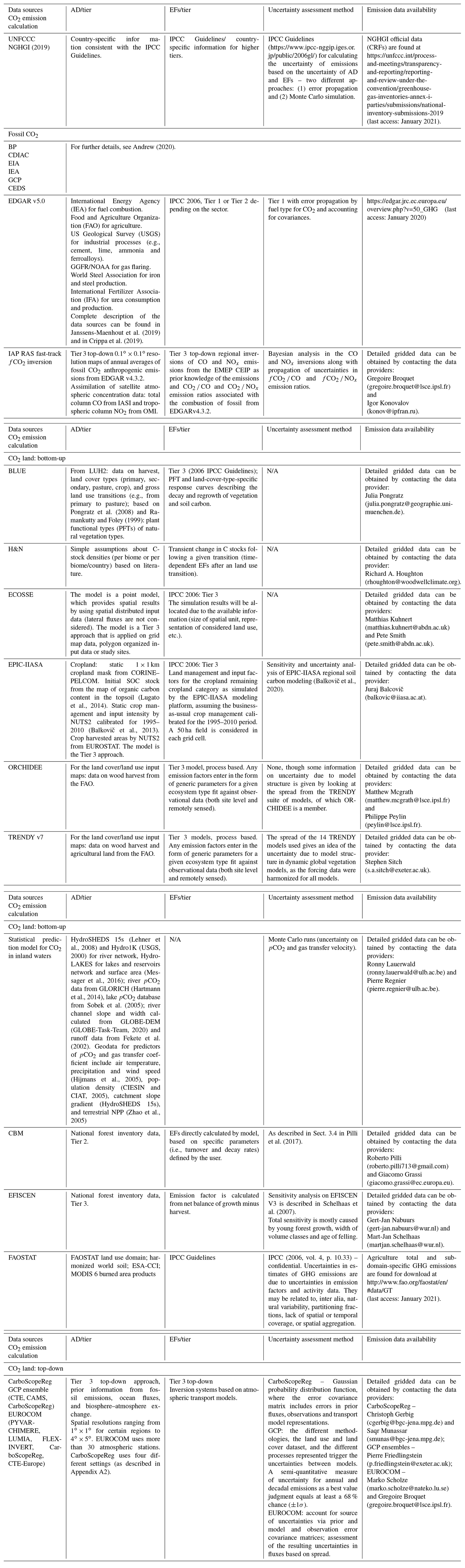
AMRP, MJM and AJD designed research and led the discussions; AMRP wrote the initial draft of the paper and edited all the following versions together with MJM, PP and AJD; RMA and MJM made the CO2 fossil figures and CO2 land figures respectively; MJM and PP processed the original data submitted to the VERIFY portal; MJM, PP and PB designed and are managing the web portal; GPP provided the Figs. B1 and B2 and performed a very detailed review of a previous version; AMRP processed the UNFCCC data and uncertainties; CQ helped make Fig. 4; HACDvdG led the initial discussions within the fossil CO2 working group and gave valuable suggestions to the manuscript structure; PC, GB, FNT, CG, JP, JMG, GG, GJN, PR, RL, MK, JB, RP, IBK, LP, PS, RLT, GC and AJD read, gave comments and advice on previous versions of the manuscript; all co-authors commented on specific parts related to their datasets; MJM, PP, PB, FNT, PR, RL, MK, JB, RP, IBK, RAH, MC, RG, IL, CG, SM, GC, GM, UK and MS are data providers.
The authors declare that they have no conflict of interest.
The views expressed in this publication are those of the author(s) and do not necessarily reflect the views or policies of FAO.
FAOSTAT statistics are produced and disseminated with the support of its member countries to the FAO regular budget. Philippe Ciais acknowledges the support of the European Research Council Synergy project SyG-2013-610028 IMBALANCE-P and from the ANR CLAND Convergence Institute. We acknowledge the work of the entire EDGAR group (Marilena Muntean, Diego Guizzardi, Edwin Schaaf and Jos Olivier). We acknowledge Stephen Sitch and the authors of the DGVMs TRENDY v7 ensemble models for providing us with the data.
This research has been supported by the H2020 European Research Council (grant no. 776810).
This paper was edited by Nellie Elguindi and reviewed by two anonymous referees.
Andrew, R. M.: Global CO2 emissions from cement production, 1928–2018, Earth Syst. Sci. Data, 11, 1675–1710, https://doi.org/10.5194/essd-11-1675-2019, 2019.
Andrew, R. M.: A comparison of estimates of global carbon dioxide emissions from fossil carbon sources, Earth Syst. Sci. Data, 12, 1437–1465, https://doi.org/10.5194/essd-12-1437-2020, 2020.
Arneth, A., Sitch, S., Pongratz, J., Stocker, B. D., Ciais, P., Poulter, B., Bayer, A. D., Bondeau, A, Calle, L., Chini, L. P., Gasser, T., Fader, M., Friedlingstein, P., Kato, E., Li, W., Lindeskog, M., Nabel, J. E. M. S., Pugh, T. A. M., Robertson, E., Viovy, N., Yue E., and Zaehle, S.: Historical carbon dioxide emissions caused by land-use changes are possibly larger than assumed, Nat. Geosci., 10, 79–84, https://doi.org/10.1038/ngeo2882, 2017.
Balkovič, J., van der Velde, M., Schmid, E., Skalský, R., Khabarov, N., Obersteiner, M., Stürmer, B., and Xiong, W.: Pan-European crop modelling with EPIC: Implementation, up-scaling and regional crop yield validation, Agr. Syst., 120, 61–75, https://doi.org/10.1016/j.agsy.2013.05.008, 2013.
Balkovič, J., Skalský, R., Folberth, C., Khabarov, N., Schmid, E., Madaras, M., Obersteiner, M., and van der Velde, M.: Impacts and Uncertainties of +2 ∘C of Climate Change and Soil Degradation on European Crop Calorie Supply, Earths Future, 6, 373–395, https://doi.org/10.1002/2017EF000629, 2018.
Balkovič, J., Madaras, M., Skalský, R., Folberth, C., Smatanová, M., Schmid, E., van der Velde, M., Kraxner, F., and Obersteiner, M.: Verifiable soil organic carbon modelling to facilitate regional reporting of cropland carbon change: A test case in the Czech Republic, J. Environ. Manage., 274, 111206, https://doi.org/10.1016/j.jenvman.2020.111206, 2020.
Bastos, A., Ciais, P., Friedlingstein, P., Sitch, S., Pongratz, J., Fan, L., Wigneron, J. P., Weber, U., Reichstein, M., Fu, Z., Anthoni, P., Arneth, A., Haverd, V., Jain, A. K., Joetzjer, E., Knauer, J., Lienert, S., Loughran, T., McGuire, P. C., Tian, H., Viovy, N., and Zaehle, S.: Direct 360 and seasonal legacy effects of the 2018 heat wave and drought on European ecosystem productivity, Science Advances, 6, eaba2724, https://doi.org/10.1126/sciadv.aba2724, 2020.
Berchet, A., Sollum, E., Thompson, R. L., Pison, I., Thanwerdas, J., Broquet, G., Chevallier, F., Aalto, T., Bergamaschi, P., Brunner, D., Engelen, R., Fortems-Cheiney, A., Gerbig, C., Groot Zwaaftink, C., Haussaire, J.-M., Henne, S., Houweling, S., Karstens, U., Kutsch, W. L., Luijkx, I. T., Monteil, G., Palmer, P. I., van Peet, J. C. A., Peters, W., Peylin, P., Potier, E., Rödenbeck, C., Saunois, M., Scholze, M., Tsuruta, A., and Zhao, Y.: The Community Inversion Framework v1.0: a unified system for atmospheric inversion studies, Geosci. Model Dev. Discuss. [preprint], https://doi.org/10.5194/gmd-2020-407, in review, 2020.
Bergamaschi, P., Karstens, U., Manning, A. J., Saunois, M., Tsuruta, A., Berchet, A., Vermeulen, A. T., Arnold, T., Janssens-Maenhout, G., Hammer, S., Levin, I., Schmidt, M., Ramonet, M., Lopez, M., Lavric, J., Aalto, T., Chen, H., Feist, D. G., Gerbig, C., Haszpra, L., Hermansen, O., Manca, G., Moncrieff, J., Meinhardt, F., Necki, J., Galkowski, M., O'Doherty, S., Paramonova, N., Scheeren, H. A., Steinbacher, M., and Dlugokencky, E.: Inverse modelling of European CH4 emissions during 2006–2012 using different inverse models and reassessed atmospheric observations, Atmos. Chem. Phys., 18, 901–920, https://doi.org/10.5194/acp-18-901-2018, 2018.
Boden, T. A., Marland, G., and Andres, R. J.: Global, Regional, and National Fossil-Fuel CO2 Emissions, Carbon Dioxide Information Analysis Center, Oak Ridge National Laboratory, U.S. Department of Energy, Oak Ridge, Tenn., USA https://doi.org/10.3334/CDIAC/00001_V2017, 2017.
BP: 60 Years BP Statistical Review of World Energy: 1951–2011, available at: https://www.bp.com/en/global/corporate/energy-economics/statistical-review-of-world-energy/downloads.html (last access: 8 February 2019), 2011.
BP: Methodology for calculating CO2 emissions from energy use, available at: https://www.bp.com/en/global/corporate/energy-economics/statistical-review-of-world-energy/co2-emissions.html (last access: 8 February 2019), 2017.
BP: BP Statistical Review of World Energy June 2018, available at: https://www.bp.com/en/global/corporate/energy-economics/statistical-review-of-world-energy.html, last access: 14 June 2018.
Bradbury, N. J., Whitmore, A. P., Hart, P. B. S., and Jenkinson, D. S.: Modelling the fate of nitrogen in crop and soil in the years following application of 15N-labelled fertilizer to winter wheat, J. Agr. Sci., 121, 363–379, 1993.
Brophy, K., Graven, H., Manning, A. J., White, E., Arnold, T., Fischer, M. L., Jeong, S., Cui, X., and Rigby, M.: Characterizing uncertainties in atmospheric inversions of fossil fuel CO2 emissions in California, Atmos. Chem. Phys., 19, 2991–3006, https://doi.org/10.5194/acp-19-2991-2019, 2019.
Carlson, D. and Oda, T.: Editorial: Data publication – ESSD goals, practices and recommendations, Earth Syst. Sci. Data, 10, 2275–2278, https://doi.org/10.5194/essd-10-2275-2018, 2018.
Chang, J., Ciais, P., Herrero, M., Havlik, P., Campioli, M., Zhang, X., Bai, Y., Viovy, N., Joiner, J., Wang, X., Peng, S., Yue, C., Piao, S., Wang, T., Hauglustaine, D. A., Soussana, J.-F., Peregon, A., Kosykh, N., and Mironycheva-Tokareva, N.: Combining livestock production information in a process-based vegetation model to reconstruct the history of grassland management, Biogeosciences, 13, 3757–3776, https://doi.org/10.5194/bg-13-3757-2016, 2016.
Chevallier, F., Fisher, M., Peylin, P., Serrar, S., Bousquet, P., Bréon, F.-M., Chédin, A., and Ciais, P.: Inferring CO2 sources and sinks from satellite observations: Method and application to TOVS data, J. Geophys. Res.-Atmos., 110, D24309, https://doi.org/10.1029/2005JD006390, 2005.
Ciais, P., Reichstein, M., Viovy, N., Granier, A., Ogée, J., Allard, V., Aubinet, M., Buchmann, N., Bernhofer, C., Carrara, A., Chevallier, F., De Noblet, N., Friend, A. D., Friedlingstein, P., Grünwald, T., Heinesch, B., Keronen, P., Knohl, A., Krinner, G., Loustau, D., Manca, G., Matteucci, G., Miglietta, F., Ourcival, J. M., Papale, D., Pilegaard, K., Rambal, S., Seufert, G., Soussana, J. F., Sanz, M. J., Schulze, E. D., Vesala, T., and Valentini, R.: Europe-wide reduction in primary productivity caused by the heat and drought in 2003, Nature, 437, 529–533, https://doi.org/10.1038/nature03972, 2005.
Ciais, P., Wattenbach, M., Vuichard, N., Smith, P., Piao, S. L., Don, A., Luyssaert, S., Janssens, A., Bondeau, A., Dechow, R., Leip, A., Smith, P. C., Beer, C., van der Werf, G. R., Gervois, S., van Oost, K., Tomelleri, E., Freibauer, A., Schulze, E. D., and Carboneurope Synthesis Team: The European carbon balance, Part 2: croplands, Global Change Biol., 16, 1409–1428, https://doi.org/10.1111/j.1365-2486.2009.02055.x, 2010.
Ciais, P., Crisp, D., Denier van der Gon, H. A. C., Engelen, R., Janssens-Maenhout, G., Heiman, M., Rayner, P., and Scholze, M.: Towards A European Operational Observing System To Monitor Fossil CO2 Emissions, Final Report from the expert group, European Commission, https://www.copernicus.eu/sites/default/files/2019-09/CO2_Blue_report_2015.pdf (last access: June 2020), 2015.
Ciais, P., Bastos, A., Chevallier, F., Lauerwald, R., Poulter, B., Canadell, P., Hugelius, G., Jackson, R. B., Jain, A., Jones, M., Kondo, M., Luijkx, I., Patra, P. K., Peters, W., Pongratz, J., Petrescu, A. M. R., Piao, S., Qiu, C., Von Randow, C., Regnier, P., Saunois, M., Scholes, R., Shvidenko, A., Tian, H., Yang, H., Wang, X., and Zheng, B.: Definitions and methods to estimate regional land carbon fluxes for the second phase of the REgional Carbon Cycle Assessment and Processes Project (RECCAP-2), Geosci. Model Dev. Discuss. [preprint], https://doi.org/10.5194/gmd-2020-259, in review, 2020.
CIESIN and CIAT: Gridded Population of the World, Version 3 (GPWv3): Population Count Grid, Palisades, NY, NASA Socioeconomic Data and Applications Center (SEDAC), Center for International Earth Science Information Network (CIESIN) and Columbia University, United Nations Food and Agriculture Programme (FAO), and Centro Internacional de Agricultura Tropical (CIAT), https://doi.org/10.7927/H4639MPP, 2005.
Coleman, K. and Jenkinson, D. S.: RothC-26.3 – A model the turnover of carbon in soil, in: Evaluation of soil organic matter models using existing long-term datasets, edited by: Powlson, D. S., Smith, P., and Smith, J. U., NATO ASI Series I, Springer, Berlin, Germany, 237–246, 1996.
Crippa, M., Oreggioni, G., Guizzardi, D., Muntean, M., Schaaf, E., Lo Vullo, E., Solazzo, E., Monforti-Ferrario, F., Olivier, J. G. J., and Vignati, E.: Fossil CO2 and GHG emissions of all world countries: 2019 Report, Publications Office of the European Union, Luxembourg, JRC117610, https://doi.org/10.2760/687800, 2019.
Ducoudré, N. I., Laval, K., and Perrier, A.: SECHIBA, a new set of parameterizations of the hydrologic exchanges at the land-atmosphere interface within the LMD atmospheric general circulation model, J. Climate, 6, 248–273, 1993.
EIA: International Energy Statistics, Energy Information Administration, available at: https://www.eia.gov/international/data/ world, last access: 4 February 2020.
EU LIFE: EU Report LIFE and Europe's grasslands Restoring a forgotten habitat, https://ec.europa.eu/environment/archives/life/publications/lifepublications/lifefocus/documents/grassland.pdf (last access: November 2020), 2008.
FAO: FAOSTAT data, available at: http://www.fao.org/faostat/en/#data (last access: January 2020), 2018.
Federici, S., Tubiello, F. N., Salvatore, M., Jacobs, H., and Schmidhuber, J.: New estimates of CO2 forest emissions and removals: 1990–2015, Forest Ecol. Manag., 352, 89–98, 2015.
Fekete, B. M., Vorosmarty, C. J., and Grabs, W.: High-resolution fields of global runoff combining observed river discharge and simulated 38 water balances, Global Biogeochem. Cy., 16, 1042, https://doi.org/10.1029/1999gb001254, 2002.
FRA: Global Forest Resources Assessment 2015: How are the world's forest changing?, Rome, Italy, http://www.fao.org/3/a-i4793e.pdf (last access: December 2019), 2015.
Frey, C.: Evaluation of an approximate analytical procedure for calculating uncertainty in the Greenhouse gas version of the multi scale motor vehicle and equipment emission system (order 3A-0419-NATX), available at: https://citeseerx.ist.psu.edu/viewdoc/download?doi=10.1.1.413.6630&rep=rep1&type=pdf (last access: January 2020), 2003.
Friedlingstein, P., Jones, M. W., O'Sullivan, M., Andrew, R. M., Hauck, J., Peters, G. P., Peters, W., Pongratz, J., Sitch, S., Le Quéré, C., Bakker, D. C. E., Canadell, J. G., Ciais, P., Jackson, R. B., Anthoni, P., Barbero, L., Bastos, A., Bastrikov, V., Becker, M., Bopp, L., Buitenhuis, E., Chandra, N., Chevallier, F., Chini, L. P., Currie, K. I., Feely, R. A., Gehlen, M., Gilfillan, D., Gkritzalis, T., Goll, D. S., Gruber, N., Gutekunst, S., Harris, I., Haverd, V., Houghton, R. A., Hurtt, G., Ilyina, T., Jain, A. K., Joetzjer, E., Kaplan, J. O., Kato, E., Klein Goldewijk, K., Korsbakken, J. I., Landschützer, P., Lauvset, S. K., Lefèvre, N., Lenton, A., Lienert, S., Lombardozzi, D., Marland, G., McGuire, P. C., Melton, J. R., Metzl, N., Munro, D. R., Nabel, J. E. M. S., Nakaoka, S.-I., Neill, C., Omar, A. M., Ono, T., Peregon, A., Pierrot, D., Poulter, B., Rehder, G., Resplandy, L., Robertson, E., Rödenbeck, C., Séférian, R., Schwinger, J., Smith, N., Tans, P. P., Tian, H., Tilbrook, B., Tubiello, F. N., van der Werf, G. R., Wiltshire, A. J., and Zaehle, S.: Global Carbon Budget 2019, Earth Syst. Sci. Data, 11, 1783–1838, https://doi.org/10.5194/essd-11-1783-2019, 2019.
Friedlingstein, P., O'Sullivan, M., Jones, M. W., Andrew, R. M., Hauck, J., Olsen, A., Peters, G. P., Peters, W., Pongratz, J., Sitch, S., Le Quéré, C., Canadell, J. G., Ciais, P., Jackson, R. B., Alin, S., Aragão, L. E. O. C., Arneth, A., Arora, V., Bates, N. R., Becker, M., Benoit-Cattin, A., Bittig, H. C., Bopp, L., Bultan, S., Chandra, N., Chevallier, F., Chini, L. P., Evans, W., Florentie, L., Forster, P. M., Gasser, T., Gehlen, M., Gilfillan, D., Gkritzalis, T., Gregor, L., Gruber, N., Harris, I., Hartung, K., Haverd, V., Houghton, R. A., Ilyina, T., Jain, A. K., Joetzjer, E., Kadono, K., Kato, E., Kitidis, V., Korsbakken, J. I., Landschützer, P., Lefèvre, N., Lenton, A., Lienert, S., Liu, Z., Lombardozzi, D., Marland, G., Metzl, N., Munro, D. R., Nabel, J. E. M. S., Nakaoka, S.-I., Niwa, Y., O'Brien, K., Ono, T., Palmer, P. I., Pierrot, D., Poulter, B., Resplandy, L., Robertson, E., Rödenbeck, C., Schwinger, J., Séférian, R., Skjelvan, I., Smith, A. J. P., Sutton, A. J., Tanhua, T., Tans, P. P., Tian, H., Tilbrook, B., van der Werf, G., Vuichard, N., Walker, A. P., Wanninkhof, R., Watson, A. J., Willis, D., Wiltshire, A. J., Yuan, W., Yue, X., and Zaehle, S.: Global Carbon Budget 2020, Earth Syst. Sci. Data, 12, 3269–3340, https://doi.org/10.5194/essd-12-3269-2020, 2020.
Gasser, T. and Ciais, P.: A theoretical framework for the net land-to-atmosphere CO2 flux and its implications in the definition of “emissions from land-use change”, Earth Syst. Dynam., 4, 171–186, https://doi.org/10.5194/esd-4-171-2013, 2013.
GLOBE-Task-Team: The Global Land one-kilometer Base Elevation (GLOBE) digital elevation model, Version 1.0, available at: http://www.ngdc.noaa.gov/mgg/topo/globe.html, last access: June 2020.
Grassi, G., House, J., Kurz, W. A., Cescatti, A., Houghton, R. A., Peters, G. P., Sanz, M. J., Viñas, R. A., Alkama, R., Arneth, A., Bondeau, A., Dentener, F., Fader, M., Federici, S., Friedlingstein, P., Jain, A. K., Kato, E., Koven, C. D., Lee, D., Nabel, J. E. M. S., Nassikas, A. A., Perugini, L., Rossi, S., Sitch, S., Viovy, N., Wiltshire, A., and Zaehle, S.: Reconciling global-model estimates and country reporting of anthropogenic forest CO2 sinks, Nat. Clim. Change, 8, 914–920, https://doi.org/10.1038/s41558-018-0283-x, 2018a.
Grassi, G., Pilli, R., House, J., Federici, S., and Kurz, W. A.: Science-based approach for credible accounting of itigation in managed forests, Carbon Balance and Management, 13, 8, https://doi.org/10.1186/s13021-018-0096-2, 2018b.
Grassi, G., Cescatti, A., Matthews, R., Duveiller, G., Amia, A., Federici, S., House, J., de Noblet-Ducoudré, N., Pilli, R., and Vizzarri, M.: On the realistic contribution of European forests to reach climate objectives, Carbon Balance and Management, 14, 8, https://doi.org/10.1186/s13021-019-0123-y, 2019.
Hansis, E., Davis, S. J., and Pongratz, J.: Relevance of methodological choices for accounting of land use change carbon fluxes, Global Biogeochem. Cy., 29, 1230–1246, https://doi.org/10.1002/2014GB004997, 2015.
Hartmann, J., Lauerwald, R., and Moosdorf, N.: A brief overview of the GLObal RIver CHemistry Database, GLORICH, Procedia Earth Planet. Sci., 10, 23–27, 2014.
Hastie, A., Lauerwald, R., Ciais, P., and Regnier, P.: Aquatic carbon fluxes dampen the overall variation of net ecosystem productivity in the Amazon basin: An analysis of the interannual variability in the boundless carbon cycle, Global Change Biol., 25, 2094–2111, https://doi.org/10.1111/gcb.14620, 2019.
Hijmans, R. J., Cameron, S. E., Parra, J. L., Jones, P. G., and Jarvis, A.: Very high resolution interpolated climate surfaces for global land areas, Int. J. Climatol., 25, 1965–1978, https://doi.org/10.1002/joc.1276, 2005.
Houghton, R. A.: Revised estimates of the annual net flux of carbon to the atmosphere from changes in land use and land management 1850–2000, Tellus B, 55, 378–390, 2003.
Houghton, R. A. and Nassikas, A. A.: Global and regional fluxes of carbon from land use and land cover change 1850–2015, Global Biogeochem. Cy., 31, 456–472, https://doi.org/10.1002/2016GB005546, 2017.
Houghton, R. A., Hobbie, J., Melillo, J., Moore, B., Peterson, B., Shaver, G., and Woodwell, G.: Changes in the carbon content of terrestrial biota and soils between 1860 and 1980: A net release of CO2 to the atmosphere, Ecol. Monogr., 53, 235–262, 1983.
Houghton, R. A., House, J. I., Pongratz, J., van der Werf, G. R., DeFries, R. S., Hansen, M. C., Le Quéré, C., and Ramankutty, N.: Carbon emissions from land use and land-cover change, Biogeosciences, 9, 5125–5142, https://doi.org/10.5194/bg-9-5125-2012, 2012.
Hurtt, G. C., Chini, L., Sahajpal, R., Frolking, S., Bodirsky, B. L., Calvin, K., Doelman, J. C., Fisk, J., Fujimori, S., Klein Goldewijk, K., Hasegawa, T., Havlik, P., Heinimann, A., Humpenöder, F., Jungclaus, J., Kaplan, J. O., Kennedy, J., Krisztin, T., Lawrence, D., Lawrence, P., Ma, L., Mertz, O., Pongratz, J., Popp, A., Poulter, B., Riahi, K., Shevliakova, E., Stehfest, E., Thornton, P., Tubiello, F. N., van Vuuren, D. P., and Zhang, X.: Harmonization of global land use change and management for the period 850–2100 (LUH2) for CMIP6, Geosci. Model Dev., 13, 5425–5464, https://doi.org/10.5194/gmd-13-5425-2020, 2020.
IEA: CO2 Emissions From Fuel Combustion: Database Documentation, International Energy Agency, Paris, France, http://wds.iea.org/wds/pdf/Worldco2_Documentation.pdf, last access: 8 February, 2019.
IPCC: Good Practice Guidance for Land use, Land use Change and Forestry, https://www.ipcc-ggip.iges.or.jp/public/gpglulucf/gpglulucf_files/GPG_LULUCF_FULL.pdf (last access: January 2020), 2003.
IPCC: 2006 Guidelines for National Greenhouse Gas Inventories, prepared by the National Greenhouse Gas Inventories Programme, IGES, Japan, available at: https://www.ipcc-nggip.iges.or.jp/public/2006gl/ (last access: December 2019), 2006.
IPCC: Supplement to the 2006 IPCC Guidelines for National Greenhouse Gas Inventories: Wetlands, edited by: Hiraishi, T., Krug, T., Tanabe, K., Srivastava, N., Baasansuren, J., Fukuda, M., and Troxler, T. G., IPCC, Switzerland, 2014.
IPCC: 2019 Refinement to the 2006 IPCC Guidelines for National Greenhouse Gas Inventories, available at: https://www.ipcc.ch/report/2019-refinement-to-the-2006-ipcc-guidelines-for-national-greenhouse-gas-inventories (last access: January 2020), 2019.
Izaurralde, R. C., Williams, J. R., McGill, W. B., Rosenberg, N. J., and Jakas, M. C. Q.: Simulating soil C dynamics with EPIC: Model description and testing against long-term data, Ecol. Model., 192, 362–384, https://doi.org/10.1016/j.ecolmodel.2005.07.010, 2006.
Janssens-Maenhout, G., Crippa, M., Guizzardi, D., Muntean, M., Schaaf, E., Dentener, F., Bergamaschi, P., Pagliari, V., Olivier, J. G. J., Peters, J. A. H. W., van Aardenne, J. A., Monni, S., Doering, U., Petrescu, A. M. R., Solazzo, E., and Oreggioni, G. D.: EDGAR v4.3.2 Global Atlas of the three major greenhouse gas emissions for the period 1970–2012, Earth Syst. Sci. Data, 11, 959–1002, https://doi.org/10.5194/essd-11-959-2019, 2019.
Janssens-Maenhout, G., Pinty, B., Dowell, M., Zunker, H., Andersson, E., Balsamo, G., Bézy, J.-L., Brunhes, T., Bösch, H., Bojkov, B., Brunner, D., Buchwitz, M., Crisp, D., Ciais, P., Counet, P., Dee, D., Denier van der Gon, H. A. C., Dolman, H., Drinkwater, M. R., Dubovik, O., Engelen, R., Fehr, T., Fernandez, V., Heimann, M., Holmlund, K., Houweling, S., Husband, R., Juvyns, O., Kentarchos, A., Landgraf, J., Lang, R., Löscher, A., Marshall, J., Meijer, Y., Nakajima, M., Palmer, P. I., Peylin, P., Rayner, P., Scholze, M., Sierk, B., Tamminen, J., and Veefkind, P.: Toward an Operational Anthropogenic CO2 Emissions Monitoring and Verification Support Capacity, B. Am. Meteorol. Soc., 101, 1439–1451, https://doi.org/10.1175/BAMS-D-19-0017.1, 2020.
Jenkinson, D. S. and Rayner, J. H.: The turnover of organic matter in some of the Rothamsted classical experiments, Soil Sci., 123, 298–305, 1977.
Jenkinson, D. S., Hart, P. B. S., Rayner, J. H., and Parry, L. C.: Modelling the turnover of organic matter in long-term experiments at Rothamsted, INTECOL Bulletin, 15, 1–8, 1987.
Jonsson, R., Blujdea, V. N., Fiorese, G., Pilli, R., Rinaldi, F., Baranzelli, C., and Camia, A.: Outlook of the European forestbased sector: forest growth, harvest demand, wood-product markets, and forest carbon dynamics implications, iForest, 11, 315–328, https://doi.org/10.3832/ifor2636-011, 2018.
Klein Goldewijk, K., Beusen, A., Doelman, J., and Stehfest, E.: Anthropogenic land use estimates for the Holocene – HYDE 3.2, Earth Syst. Sci. Data, 9, 927–953, https://doi.org/10.5194/essd-9-927-2017, 2017a.
Klein Goldewijk, K., Dekker, S. C., and van Zanden, J. L.: Percapita estimations of long-term historical land use and the consequences for global change research, J. Land Use Sci., 12, 313–337, https://doi.org/10.1080/1747423X.2017.1354938, 2017b.
Koehl, M., Hildebrandt, R., Olschofsky, K., Koehler, R., Roetzer, T., Mette, T., Pretzsch, H., Koethke, M., Dieter, M., Abiy, M., Makeschin, F., and Kenter, B.: Combating the effects of climatic change on forests by mitigation strategies, Carbon Balance and Management, 5, 8, https://doi.org/10.1186/1750-0680-5-8, 2010.
Konovalov, I. B. and Lvova, D. A.: First, fast-track, Re-analysis of the national scale CO2 anthropogenic emissions over 2005–2015, internal VERIFY report: https://projectsworkspace.eu/sites/VERIFY/Deliverables/WP2/ VERIFY_D2.10_First, fast-track, Re-analysis of the national scale CO$_2$ anthropogenic emissions over 2005-2015.pdf (last access September 2020), 2018.
Konovalov, I. B., Berezin, E. V., Ciais, P., Broquet, G., Zhuravlev, R. V., and Janssens-Maenhout, G.: Estimation of fossil-fuel CO2 emissions using satellite measurements of “proxy” species, Atmos. Chem. Phys., 16, 13509–13540, https://doi.org/10.5194/acp-16-13509-2016, 2016.
Kountouris, P., Gerbig, C., Rödenbeck, C., Karstens, U., Koch, T. F., and Heimann, M.: Technical Note: Atmospheric CO2 inversions on the mesoscale using data-driven prior uncertainties: methodology and system evaluation, Atmos. Chem. Phys., 18, 3027–3045, https://doi.org/10.5194/acp-18-3027-2018, 2018a.
Kountouris, P., Gerbig, C., Rödenbeck, C., Karstens, U., Koch, T. F., and Heimann, M.: Atmospheric CO2 inversions on the mesoscale using data-driven prior uncertainties: quantification of the European terrestrial CO2 fluxes, Atmos. Chem. Phys., 18, 3047–3064, https://doi.org/10.5194/acp-18-3047-2018, 2018b.
Krinner, G., Viovy, N., de Noblet-Ducoudré N., Ogée, J., Polcher, J., Friedlingstein, P., Ciais, P., Sitch, S., and Prentice, I. C.: A dynamic global vegetation model for studies of the coupled atmosphere-biosphere system, Global Biogeochem. Cy., 19, GB1015, https://doi.org/10.1029/2003GB002199, 2005.
Kurz, W. A.: Large inter-annual variations in carbon emissions and removals, Invited Background Paper, in: IPCC 2010, Revisiting the Use of Managed Land as a Proxy for Estimating National Anthropogenic Emissions and Removals, edited by: Eggleston, H. S., Srivastava, N., Tanabe, K., and Baasansuren, J., INPE, Sao José dos Campos, Brazil, 5–7 May 2009, IGES, Hayama, Japan, 41–48, 2010.
Kurz, W. A., Dymond, C. C., White, T. M., Stinson, G., Shaw, C. H., Rampley, G. J., Smyth, C., Simpson, B. N., Neilson, E. T., Trofymow, J. A., Metsaranta, J., and Apps, M. J.: CBMCFS3:a model of carbon-dy-namics in forestry and land use change imple-menting IPCC standards, Ecol. Model., 220, 480–504, https://doi.org/10.1016/j.ecolmodel.2008.10.018, 2009.
Lauerwald, R., Laruelle, G. G., Hartmann, J., Ciais, P., and Regnier, P. A. G.: Spatial patterns in CO2 evasion from the global river network, Global Biogeochem. Cy., 29, 534–554, https://doi.org/10.1002/2014GB004941015, 2015.
Lehner, B., Verdin, K., and Jarvis, A.: New global hydrography derived from spaceborne elevation data, EOS T. Am. Geophys. Un., 89, 93–94, https://doi.org/10.1029/2008EO100001, 2008.
Le Quéré, C., Raupach, M. R., Canadell, J. G., Marland, G., Bopp, L., Ciais, P., Conway, T. J., Doney, S. C., Feely, R. A., Foster, P., Friedlingstein, P., Gurney, K., Houghton, R. A., House, J. I., Huntingford, C., Levy, P. E., Lomas, M. R., Majkut, J., Metzl, N., Ometto, J. P., Peters, G. P., Prentice, I. C., Randerson, J. T., Running, S. W., Sarmiento, J. L., Schuster, U., Sitch, S., Takahashi, T., Viovy, N., van der Werf, G. R., and Woodward, F. I.: Trends in the sources and sinks of carbon dioxide, Nat. Geosci., 2, 831–836, 2009.
Le Quéré, C., Andrew, R. M., Friedlingstein, P., Sitch, S., Pongratz, J., Manning, A. C., Korsbakken, J. I., Peters, G. P., Canadell, J. G., Jackson, R. B., Boden, T. A., Tans, P. P., Andrews, O. D., Arora, V. K., Bakker, D. C. E., Barbero, L., Becker, M., Betts, R. A., Bopp, L., Chevallier, F., Chini, L. P., Ciais, P., Cosca, C. E., Cross, J., Currie, K., Gasser, T., Harris, I., Hauck, J., Haverd, V., Houghton, R. A., Hunt, C. W., Hurtt, G., Ilyina, T., Jain, A. K., Kato, E., Kautz, M., Keeling, R. F., Klein Goldewijk, K., Körtzinger, A., Landschützer, P., Lefèvre, N., Lenton, A., Lienert, S., Lima, I., Lombardozzi, D., Metzl, N., Millero, F., Monteiro, P. M. S., Munro, D. R., Nabel, J. E. M. S., Nakaoka, S., Nojiri, Y., Padin, X. A., Peregon, A., Pfeil, B., Pierrot, D., Poulter, B., Rehder, G., Reimer, J., Rödenbeck, C., Schwinger, J., Séférian, R., Skjelvan, I., Stocker, B. D., Tian, H., Tilbrook, B., Tubiello, F. N., van der Laan-Luijkx, I. T., van der Werf, G. R., van Heuven, S., Viovy, N., Vuichard, N., Walker, A. P., Watson, A. J., Wiltshire, A. J., Zaehle, S., and Zhu, D.: Global Carbon Budget 2017, Earth Syst. Sci. Data, 10, 405–448, https://doi.org/10.5194/essd-10-405-2018, 2018.
Liski, J., Karjalainen, T., Pussinen, A., Nabuurs, G.-J., and Kauppi, P.: Trees as carbon sinks and sources in the European Union, Environ. Sci. Policy, 3, 91–97, https://doi.org/10.1016/S1462-9011(00)00020-4, 2000.
Liski, J., Palosuo, T., Peltoniemi, M., and Sievänen, R.: Carbon and decomposition model Yasso for forest soils, Ecol. Model., 189, 168–182, https://doi.org/10.1016/J.ECOLMODEL.2005.03.005, 2005.
Lugato, E., Panagos, P., Bampa, F., Jones, A., and Montanarella, L.: A new baseline of organic carbon stock in European agricultural soils using a modelling approach, Global Change Biol., 20, 313–326, https://doi.org/10.1111/gcb.12292, 2014.
Lurton, T., Balkanski, Y., Bastrikov, V., Bekki, S., Bopp, L., Braconnot, P., and Cugnet, D.: Implementation of the CMIP6 Forcing Data in the IPSL-CM6A-LR Model, J. Adv. Model. Earth Sy., 12, e2019MS001940, https://doi.org/10.1029/2019MS001940, 2020.
Luyssaert, S., Abril, G., Andres, R., Bastviken, D., Bellassen, V., Bergamaschi, P., Bousquet, P., Chevallier, F., Ciais, P., Corazza, M., Dechow, R., Erb, K.-H., Etiope, G., Fortems-Cheiney, A., Grassi, G., Hartmann, J., Jung, M., Lathière, J., Lohila, A., Mayorga, E., Moosdorf, N., Njakou, D. S., Otto, J., Papale, D., Peters, W., Peylin, P., Raymond, P., Rödenbeck, C., Saarnio, S., Schulze, E.-D., Szopa, S., Thompson, R., Verkerk, P. J., Vuichard, N., Wang, R., Wattenbach, M., and Zaehle, S.: The European land and inland water CO2, CO, CH4 and N2O balance between 2001 and 2005, Biogeosciences, 9, 3357–3380, https://doi.org/10.5194/bg-9-3357-2012, 2012.
Luyssaert, S., Marie, G., Valade, A., Chen, Y. Y., Njakou Djomo, S., Ryder, J., Otto, J., Naudts, K., Lansø, A. S., Ghattas, J., and McGrath, M. J.: Trade-offs in using European forests to meet climate objectives, Nature, 562, 259–262, https://doi.org/10.1038/s41586-018-0577-1, 2018.
Menut, L., Bessagnet, B., Khvorostyanov, D., Beekmann, M., Blond, N., Colette, A., Coll, I., Curci, G., Foret, G., Hodzic, A., Mailler, S., Meleux, F., Monge, J.-L., Pison, I., Siour, G., Turquety, S., Valari, M., Vautard, R., and Vivanco, M. G.: CHIMERE 2013: a model for regional atmospheric composition modelling, Geosci. Model Dev., 6, 981–1028, https://doi.org/10.5194/gmd-6-981-2013, 2013.
Messager, M. L., Lehner, B., Grill, G., Nedeva, I., and Schmitt, O.: Estimating the volume and age of water stored in global lakes using a geo-statistical approach, Nat. Commun., 7, 13603, https://doi.org/10.1038/ncomms13603, 2016.
Monteil, G., Broquet, G., Scholze, M., Lang, M., Karstens, U., Gerbig, C., Koch, F.-T., Smith, N. E., Thompson, R. L., Luijkx, I. T., White, E., Meesters, A., Ciais, P., Ganesan, A. L., Manning, A., Mischurow, M., Peters, W., Peylin, P., Tarniewicz, J., Rigby, M., Rödenbeck, C., Vermeulen, A., and Walton, E. M.: The regional European atmospheric transport inversion comparison, EUROCOM: first results on European-wide terrestrial carbon fluxes for the period 2006–2015, Atmos. Chem. Phys., 20, 12063–12091, https://doi.org/10.5194/acp-20-12063-2020, 2020.
Nabuurs, G. J., Delacote, P., Ellison, D., Hanewinkel, M., Hetemäki, L., Lindner, M., and Ollikainen, M.: By 2050 the mitigation effects of EU forests could nearly double through climate smart forestry, Forests, 8, 484, https://doi.org/10.3390/f8120484, 2017.
Nabuurs, G. J., Arets, E. J. M. M., and Schelhaas, M. J.: Understandin the implications of the EU-LULUCF regulation for the wood supply from EU forests to the EU, Carbon Balance and Management, 13, 18, https://doi.org/10.3390/f8120484, 2018.
Naudts, K., Chen, Y., McGrath, M., Ryder, J., Valade, A., Otto, J., and Luyssaert, S.: Europe's forest management did not mitigate climate warming, Science, 351, 597–600, https://doi.org/10.1126/science.aad7270, 2016.
Olivier, J. G. J., Schure, K. M., and Peters, J. A. H. W.: Trends in global CO2 and total greenhouse gas emissions: 2017 report, PBL Netherlands Environmental Assessment Agency, The Hague, PBL Publishers, available at: https://www.pbl.nl/sites/default/files/downloads/pbl-2017-trends-in-global-co2-and-total-greenhouse-gas-emissons-2017-report_2674_0.pdf (last access: September 2019), 2017.
Peters, G. P., Marland, G., Hertwich, E. G., Saikku, L., Rautiainen, A., and Kauppi, P. E.: Trade, Transport, and Sinks Extend the Carbon Dioxide Responsibility of Countries, Clim. Change, 97, 379–388, 2009.
Petrescu, A. M. R., McGrath, M. J., Andrew, R. M., Peylin, P., Peters, G. P., Ciais, P., Broquet, G., Tubiello, F. N., Gerbig, C., Pongratz, J., Janssens-Maenhout, G., Grassi, G., Nabuurs, G. J., Regnier, P., Lauerwald, R., Kuhnert, M., Balkovič, J., Schelhaas, M. J., Denier van der Gon, H. A. C., Solazzo, E., Qiu, C., Pilli, R., Konovalov, I. B., Houghton, R. A., Günther, D., Perugini, L., Crippa, M., Ganzenmüller, R., Luijkx, I. T., Smith, P., Munassar, S., Thompson, R. L., Conchedda, G., Monteil, G., Scholze, M., Karstens, U., Brockmann, P., and Dolman, A. J.: The consolidated European synthesis of CO2 emissions and removals for EU27 and UK: 1990–2018, version 2, Zenodo, https://doi.org/10.5281/zenodo.4626578, 2020a.
Petrescu, A. M. R., Peters, G. P., Janssens-Maenhout, G., Ciais, P., Tubiello, F. N., Grassi, G., Nabuurs, G.-J., Leip, A., Carmona-Garcia, G., Winiwarter, W., Höglund-Isaksson, L., Günther, D., Solazzo, E., Kiesow, A., Bastos, A., Pongratz, J., Nabel, J. E. M. S., Conchedda, G., Pilli, R., Andrew, R. M., Schelhaas, M.-J., and Dolman, A. J.: European anthropogenic AFOLU greenhouse gas emissions: a review and benchmark data, Earth Syst. Sci. Data, 12, 961–1001, https://doi.org/10.5194/essd-12-961-2020, 2020b.
Petrescu, A. M. R., Qiu, C., Ciais, P., Thompson, R. L., Peylin, P., McGrath, M. J., Solazzo, E., Janssens-Maenhout, G., Tubiello, F. N., Bergamaschi, P., Brunner, D., Peters, G. P., Höglund-Isaksson, L., Regnier, P., Lauerwald, R., Bastviken, D., Tsuruta, A., Winiwarter, W., Patra, P. K., Kuhnert, M., Oreggioni, G. D., Crippa, M., Saunois, M., Perugini, L., Markkanen, T., Aalto, T., Groot Zwaaftink, C. D., Yao, Y., Wilson, C., Conchedda, G., Günther, D., Leip, A., Smith, P., Haussaire, J.-M., Leppänen, A., Manning, A. J., McNorton, J., Brockmann, P., and Dolman, A. J.: The consolidated European synthesis of CH4 and N2O emissions for the European Union and United Kingdom: 1990–2017, Earth Syst. Sci. Data, 13, 2307–2362, https://doi.org/10.5194/essd-13-2307-2021, 2021.
Pilli, R., Grassi, G., Kurz, W. A., Moris, J. V., and Viñas, R. A.: Modelling forest carbon stock changes as affected by harvest and natural disturbances – II. EU-level analysis including land use changes, Carbon Balance and Management, 11, 20, https://doi.org/10.1186/s13021-016-0059-4, 2016.
Pilli, R., Grassi, G., Kurz, W. A., Fiorese, G., and Cescatti, A.: The European forest sector: past and future carbon budget and fluxes under different management scenarios, Biogeosciences, 14, 2387–2405, https://doi.org/10.5194/bg-14-2387-2017, 2017.
Polcher, J., McAvaney, B., Viterbo, P., Gaertner, M.-A., Hahmann, A., Mahfouf, J.-F., Noilhan, J., Phillips, T., Pitman, A. J., Schlosser, C. A., Schulz, J.-P., Timbal, B., Verseghy, D., and Xue, Y.: A proposal for a general interface between land-surface schemes and general circulation models, Global Planet. Change, 19, 263–278, 1998.
Pongratz, J., Reick, C., Raddatz, T., and Claussen, M.: A reconstruction of global agricultural areas and land cover for the last millennium, Global Biogeochem. Cy., 22, GB3018, https://doi.org/10.1029/2007GB003153, 2008.
Pongratz, J., Reick, C. H., Houghton, R. A., and House, J. I.: Terminology as a key uncertainty in net land use and land cover change carbon flux estimates, Earth Syst. Dynam., 5, 177–195, https://doi.org/10.5194/esd-5-177-2014, 2014.
Ramankutty, N. and Foley, J. A.: Estimating historical changes inglobal land cover: Croplands from 1700 to 1992, Global Biogeochem. Cy., 13, 997–1027, 1999.
Raymond, P. A., Hartmann, J., Lauerwald, R., Sobek, S., McDonald, C., Hoover, M., and Guth, P.: Global carbon dioxide emissions from inland waters, Nature, 503, 355–359, https://doi.org/10.1038/nature12760, 2013.
Rayner, P. J., Michalak, A. M., and Chevallier, F.: Fundamentals of data assimilation applied to biogeochemistry, Atmos. Chem. Phys., 19, 13911–13932, https://doi.org/10.5194/acp-19-13911-2019, 2019.
RECCAP: https://www.globalcarbonproject.org/Reccap/index.htm, last access November 2020.
Regulation (EU) 2018/1999 of the European Parliament and of the Council, Official Journal of the European Union, available at: https://eur-lex.europa.eu/legal-content/EN/TXT/PDF/?uri=CELEX:32018R1999&from=EN, last access November 2020.
Regulation (EU) 525/2013 of the European Parliament and of the Council, Official Journal of the European Union, available at: https://eur-lex.europa.eu/legal-content/EN/TXT/PDF/?uri=CELEX:32013R0525&from=EN, last access: November 2020.
Reichstein, M., Bahn, M., Ciais, P., Frank, D., Mahecha, M. D., Seneviratne, S. I., Zscheischler, J., Beer, C., Buchmann, N., Frank, D. C., Papale, D., Rammig, A., Smith, P., Thonicke, K., van der Velde, M., Vicca, S., Walz, A., and Wattenbach, M.: Climate extremes and the carbon cycle, Nature, 500, 287–295, https://doi.org/10.1038/nature12350, 2013.
Rödenbeck, C.: Estimating CO2 sources and sinks from atmospheric mixing ratio measurements using a global inversion of atmospheric transport, Tech. Rep. 6, Max Planck Institute for Biogeochemistry, Jena, Germany, 2005.
Sallnäs, O.: A matrix model of the Swedish forest, Studia Forestalia Suecica No. 183-1990, 23 pp., 1990.
Scharnweber, T., Smiljanic, M., Cruz-García, R., Manthey, M., and Wilmking, M.: Tree growth at the end of the 21st century – the extreme years 2018/2019 as template for future growth conditions, Environ. Res. Lett., 15, 074022, https://doi.org/10.1088/1748-9326/ab865d, 2020.
Schelhaas, M.-J., Nabuurs, G.-J., Verkerk, P. J., Hengeveld, G., Packalen, T., Sallnäs, O., Pilli, R., Grassi, G., Forsell, N., Frank, S., Gusti, M., and Havlik, P.: Forest Resource Projection Tools at the European Level, in: Forest Inventory-based Projection Systems for Wood and Biomass Availability, edited by: Barreiro, S., Schelhaas, M.-J., McRoberts, R. E., and Kändler, G., Springer International Publishing, Cham, Switzerland, 49–68, 2017.
Schlamadinger, B. and Marland, G.: The role of forest and bioenergy strategies in the global carbon cycle, Biomass Bioenerg., 10, 275–300, 1996.
Searchinger, T. D., Wirsenius, S., Beringer, T., and Dumas, P.: Assessing the efficiency of land use changes for mitigating climate change, Nature, 564, 249–253, https://doi.org/10.1038/s41586-018-0757-z, 2018.
Sitch, S., Huntingford, C., Gedney, N., Levy, P. E., Lomas, M., Piao, S. L., Betts, R., Ciais, P., Cox, P., Friedlingstein, P., Jones, C. D., Prentice, J. C., and Woodward, F. I.: Evaluation of the terrestrial carbon cycle, future plant geography and climate-carbon cycle feedbacks using five Dynamic Global Vegetation Models (DGVMs), Global Change Biol., 14, 2015–2039, 2008.
Smith, J. U., Bradbury, N. J., and Addiscott, T. M.: SUNDIAL: A PC-based system for simulating nitrogen dynamics in arable land, Agron J., 88, 38–43, 1996.
Smith, J. U., Gottschalk, P., Bellarby, J., Chapman, S., Lilly, A., Towers, W., Bell, J., Coleman, K., Nayak, D. R., Richards, M. I., Hillier, J., Flynn, H. C., Wattenbach, M., Aitkenhead, M., Yeluripurti, J. B., Farmer, J., Milne, R., Thomson, A., Evans, C., Whitmore, A. P., Falloon, P., and Smith, P.: Estimating changes in national soil carbon stocks using ECOSSE – a new model that includes upland organic soils – Part I. Model description and uncertainty in national scale simulations of Scotland, Clim. Res., 45, 179–192, https://doi.org/10.3354/cr00899, 2010a.
Smith, J. U., Gottschalk, P., Bellarby, J., Chapman, S., Lilly, A., Towers, W., Bell, J., Coleman, K., Nayak, D. R., Richards, M. I., Hillier, J., Flynn, H. C., Wattenbach, M., Aitkenhead, M., Yeluripurti, J. B., Farmer, J., Milne, R., Thomson, A., Evans, C., Whitmore, A. P., Falloon, P., and Smith, P.: Estimating changes in national soil carbon stocks using ECOSSE – a new model that includes upland organic soils – Part II. Application in Scotland, Clim. Res., 45, 193–205, https://doi.org/10.3354/cr00902, 2010b.
Sobek, S., Tranvik, L. J., and Cole, J. J.: Temperature independence of carbon dioxide supersaturation in global lakes, Global Biogeochem. Cy., 19, GB2003, https://doi.org/10.1029/2004GB002264, 2005.
Thompson, R. L., Broquet, G., Gerbig, C., Koch, T., Lang, M., Monteil, G., Munassar, S., Nickless, A., Scholze, M., Ramonet, M., Karstens, U., van Schaik, E., Wu, Z., and Rödenbeck, C.: Changes in net ecosystem exchange over Europe during the 2018 drought based on atmospheric observations, Philos. T. Roy. Soc. B, 375, 20190512, https://doi.org/10.1098/rstb.2019.0512, 2020.
Tubiello, F. N.: Greenhouse Gas Emissions Due to Agriculture, Encyclopedia of Food Security and Sustainability, 1, 196–205, https://doi.org/10.1016/B978-0-08-100596-5.21996-3, 2019.
Tubiello, F. N., Conchedda, G., Wanner, N., Federici, S., Rossi, S., and Grassi, G.: Carbon emissions and removals from forests: new estimates, 1990–2020, Earth Syst. Sci. Data, 13, 1681–1691, https://doi.org/10.5194/essd-13-1681-2021, 2021.
UNFCCC: Kyoto Climte Change Decision, available at: https://unfccc.int/process-and-meetings/conferences/past-conferences/kyoto-climate-change-conference-december-1997/decisions-kyoto-climate-change-conference-december-1997 (last access: October 2020), 1997.
UNFCCC: Decision 24/CP.19 Revision of the UNFCCC reporting guidelines on annual inventories for Parties included in Annex I to the Convention, FCCC/CP/2013/10/Add.3, 2014.
UNFCCC: National Inventory Submissions 2018, available at: https://unfccc.int/process-and-eetings/transparencyand-reporting/reporting-and-review-under-theconvention/greenhouse-gas-inventories-annex-i-parties/nationalinventory-submissions-2018 (last access: January 2020), 2018.
UNFCCC NGHGI: NIR reports: UNFCCC: National Inventory Submissions 2018, available at: https://unfccc.int/process-and-meetings/transparencyand-reporting/reporting-and-review-under-theconvention/greenhouse-gas-inventories-annex-i-parties/nationalinventory-submissions-2018 (last access: January 2020), 2018.
UNFCCC NGHGI: CRFs: available at: https://unfccc.int/process-and-meetings/transparency-and-reporting/reporting-and-review-under-the-convention/greenhouse-gas-inventories-annex-i-parties/national-inventory-submissions-2019 (last access: September 2020), 2019.
Valentini, R., Matteucci, G., Dolman, A. J., Schulze, E. D., Rebmann, C., Moors, E. J., Granier, A., Gross, P., Jensen, N. O., Pilegaard, K., Lindroth, A., Grelle, A., Bernhofer, C., Grunwald, T., Aubinet, M., Ceulemans, R., Kowalski, A. S., Vesala, T., Rannik, Ü., Berbigier, P., Loustau, D., Guomundsson J., Thorgeirsson, H., Ibrom, A., Morgenstern, K., Clement, R., Moncrieff, J., Montagnani, L., Minerbi, S., and Jarvis, P. G.: Respiration as the main determinant of carbon balance in European forests, Nature, 404, 861–865, https://doi.org/10.1038/35009084, 2000.
van der Laan-Luijkx, I. T., van der Velde, I. R., van der Veen, E., Tsuruta, A., Stanislawska, K., Babenhauserheide, A., Zhang, H. F., Liu, Y., He, W., Chen, H., Masarie, K. A., Krol, M. C., and Peters, W.: The CarbonTracker Data Assimilation Shell (CTDAS) v1.0: implementation and global carbon balance 2001–2015, Geosci. Model Dev., 10, 2785–2800, https://doi.org/10.5194/gmd-10-2785-2017, 2017.
Verkerk, P. J., Schelhaas, M.-J., Immonen, V., Hengeveld, G., Kiljunen, J., Lindner, M., Nabuurs, G.-J., Suominen, T., and Zudin, S.: Manual for the European Forest Information Scenario model (EFISCEN 4.1), EFI Technical Report 99, European Forest Institute, Finland, 49 pp., 2016.
Viovy, N.: Interannuality and CO2 sensitivity of the SECHIBA-BGC coupled SVAT-BGC model, Phys. Chem. Earth, 21, 489–497, 1996.
Williams, J. R.: The Erosion-Productivity Impact Calculator (EPIC) Model: A Case History, Philos. T. Roy. Soc. B, 329, 421–428, https://doi.org/10.1098/rstb.1990.0184, 1990.
WMO: United in Science Report, available at: https://public.wmo.int/en/resources/united_in_science (last access: January 2020), 2019.
Zhao, M., Heinsch, F. A., Nemani, R. R., and Running, S. W.: Improvements of the MODIS terrestrial gross and net primary pro- duction global data set, Remote Sens. Environ., 95, 164–176, https://doi.org/10.1016/j.rse.2004.12.011, 2005.
Annex I Parties include the industrialized countries that were members of the OECD (Organization for Economic Co-operation and Development) in 1992 plus countries with economies in transition (the EIT Parties), including the Russian Federation, the Baltic states, and several central and eastern European states (UNFCCC, https://unfccc.int/parties-observers, last access: February 2020).
For most Annex I Parties, the historical base year is 1990. However, parties included in Annex I with an economy in transition during the early 1990s (EIT Parties) were allowed to choose 1 year up to a few years before 1990 as reference because of a non-representative collapse during the breakup of the Soviet Union (e.g., Bulgaria, 1988; Hungary, 1985–1987; Poland, 1988; Romania, 1989; and Slovenia, 1986).
In the IPCC AR5 AFOLU stands for agriculture, forestry and other land use and represents a new sector replacing the two AR4 sectors Agriculture and LULUCF
The IPCC Good Practice Guidance (GPG) for Land Use, Land Use Change and Forestry (IPCC, 2003) describes a uniform structure for reporting emissions and removals of greenhouse gases. This format for reporting can be seen as land based; all land in the country must be identified as having remained in one of six classes since a previous survey or as having changed to a different (identified) class in that period. According to the IPCC SRCCL, land covers “the terrestrial portion of the biosphere that comprises the natural resources (soil, near-surface air, vegetation and other biota, and water), the ecological processes, topography, and human settlements and infrastructure that operate within that system”. Some communities prefer “biogenic” to describe these fluxes, while others found this confusing as fluxes from unmanaged forests, for example, are biogenic but not included in inventories reported to the UNFCCC. As this comparison is central to our work, we decided that “land” as defined by the IPCC was a good compromise.
According to the 2006 IPCC Guidelines the LULUCF sector includes six management classes (forest land, cropland, grassland, wetlands, settlements and other land).
According to the 2006 IPCC Guidelines, land should be reported in a “conversion” category for 20 years and then moved to a “remaining” category, unless a further change occurs. Converted land refers to CO2 emissions from conversions to and from all six classes that occurred in the previous 20 years.
Converted land refers to CO2 emissions from conversions to and from all six classes that occurred in the previous 20 years.
3G and 3H refer to UNFCCC sector activities, as reported by the standardized common reporting format (CRF) tables, which contain CO2 emissions from agricultural activities: liming and urea applications.
For BP, the method description allows for emissions from natural gas to be calculated from BP's energy data, but the data for solid and liquid fuels are insufficiently disaggregated to allow replication of BP's emissions calculation method for those fuels.
EDGAR v5.0 provides significant sectoral disaggregation of emissions, but not by fuel type due to license restrictions with the underlying energy data from the IEA.
The EU11 members are Portugal, Spain, France, Belgium, Luxembourg, the Netherlands, the United Kingdom, Germany, Denmark, Italy and Austria
In NGHGI reporting, land in the EU is considered to be managed.
Positive percentages represent sources.
Negative percentages represent sinks.
The Global Forest Resources Assessment (FRA) is the supplementary source of forest land data disseminated in FAOSTAT http://www.FAO.org/forestry/fra/en/ (last access: December 2019).
The 2006 IPCC Guidelines largely follow the definition of Histosols by the Food and Agriculture Organization (FAO) but have omitted the thickness criterion from the FAO definition to allow for often historically determined, country-specific definitions of organic soils (see Annex 3A.5, chap. 3, vol. 4 of the 2006 IPCC Guidelines for National Greenhouse Gas Inventories (2006 IPCC Guidelines) and chap. 1, Sect. 1.2 (Note 3) of the 2013 Supplement to the 2006 IPCC Guidelines for National Greenhouse Gas Inventories: Wetlands (Wetlands Supplement, IPCC 2014): https://www.ipcc-nggip.iges.or.jp/public/wetlands/pdf/Wetlands_separate_ files/WS_Chp1_Introduction.pdf, last access: June 2020).
According to the 2006 IPCC Guidelines the reporting is done for the five LULUCF carbon pools: aboveground biomass, belowground biomass, dead wood, litter and soil organic matter
CO2M: Copernicus Anthropogenic Carbon Dioxide Monitoring, https://esamultimedia.esa.int/docs/EarthObservation/CO2M_MRD_v3.0_20201001_Issued.pdf (last access: January 2021)
The last revision was made by COP 19 in 2013 (UNFCCC, 2013).
- Abstract
- Introduction
- CO2 data sources and estimation approaches
- Results and discussion
- Data availability
- Summary and concluding remarks
- Appendix A: Data sources, methodology and uncertainty descriptions
- Appendix B
- Author contributions
- Competing interests
- Disclaimer
- Acknowledgements
- Financial support
- Review statement
- References
- Article
(3058 KB) - Full-text XML
- Abstract
- Introduction
- CO2 data sources and estimation approaches
- Results and discussion
- Data availability
- Summary and concluding remarks
- Appendix A: Data sources, methodology and uncertainty descriptions
- Appendix B
- Author contributions
- Competing interests
- Disclaimer
- Acknowledgements
- Financial support
- Review statement
- References