the Creative Commons Attribution 4.0 License.
the Creative Commons Attribution 4.0 License.
 | 19 May 2021
The first pan-Alpine surface-gravity database, a modern compilation that crosses frontiers
Pavol Zahorec
Juraj Papčo
Roman Pašteka
Miroslav Bielik
Sylvain Bonvalot
Carla Braitenberg
Jörg Ebbing
Gerald Gabriel
Andrej Gosar
Adam Grand
Hans-Jürgen Götze
György Hetényi
Nils Holzrichter
Edi Kissling
Urs Marti
Bruno Meurers
Jan Mrlina
Ema Nogová
Alberto Pastorutti
Corinne Salaun
Matteo Scarponi
Josef Sebera
Lucia Seoane
Peter Skiba
Eszter Szűcs
Matej Varga
The AlpArray Gravity Research Group (AAGRG), as part of the European AlpArray program, focuses on the compilation of a homogeneous surface-based gravity data set across the Alpine area. In 2017 10 European countries in the Alpine realm agreed to contribute with gravity data for a new compilation of the Alpine gravity field in an area spanning from 2 to 23∘ E and from 41 to 51∘ N. This compilation relies on existing national gravity databases and, for the Ligurian and the Adriatic seas, on shipborne data of the Service Hydrographique et Océanographique de la Marine and of the Bureau Gravimétrique International. Furthermore, for the Ivrea zone in the Western Alps, recently acquired data were added to the database. This first pan-Alpine gravity data map is homogeneous regarding input data sets, applied methods and all corrections, as well as reference frames.
Here, the AAGRG presents the data set of the recalculated gravity fields on a 4 km × 4 km grid for public release and a 2 km × 2 km grid for special request. The final products also include calculated values for mass and bathymetry corrections of the measured gravity at each grid point, as well as height. This allows users to use later customized densities for their own calculations of mass corrections. Correction densities used are 2670 kg m−3 for landmasses, 1030 kg m−3 for water masses above the ellipsoid and −1640 kg m−3 for those below the ellipsoid and 1000 kg m−3 for lake water masses. The correction radius was set to the Hayford zone O2 (167 km). The new Bouguer anomaly is station completed (CBA) and compiled according to the most modern criteria and reference frames (both positioning and gravity), including atmospheric corrections. Special emphasis was put on the gravity effect of the numerous lakes in the study area, which can have an effect of up to 5 mGal for gravity stations located at shorelines with steep slopes, e.g., for the rather deep reservoirs in the Alps. The results of an error statistic based on cross validations and/or “interpolation residuals” are provided for the entire database. As an example, the interpolation residuals of the Austrian data set range between about −8 and +8 mGal and the cross-validation residuals between −14 and +10 mGal; standard deviations are well below 1 mGal. The accuracy of the newly compiled gravity database is close to ±5 mGal for most areas.
A first interpretation of the new map shows that the resolution of the gravity anomalies is suited for applications ranging from intra-crustal- to crustal-scale modeling to interdisciplinary studies on the regional and continental scales, as well as applications as joint inversion with other data sets. The data are published with the DOI https://doi.org/10.5880/fidgeo.2020.045 (Zahorec et al., 2021) via GFZ Data Services.
- Article
(30931 KB) - Full-text XML
-
Supplement
(15819 KB) - BibTeX
- EndNote


There is a long history of geological and geophysical research on the Alpine orogen, the results of which point to two main groups of complexity. The first is the temporal evolution of the mountain belt, with plates, terrains and units of different size and level of deformation mostly investigated from the geological record (e.g., Handy et al., 2010). This inheritance directly influences the second level of complexity, which is structural and characterizes every level of the lithosphere from sedimentary basins to orogenic roots and also the upper mantle. The level of along-strike variability of the Alps exceeds what is known in other mountain belts such as the Andes and the Himalayas (Oncken et al., 2006; Hetényi et al., 2016) and explains why some of the orogenic processes operating in the Alps are still debated.
Structural complexity at depth, and thus the advancement of our understanding of orogeny, can be resolved by high-resolution 3D geophysical imaging. This is among the primary goals of the AlpArray program and its main seismological imaging tool, the AlpArray Seismic Network. This modern array has used over 628 sites for more than 39 months across the greater Alpine area such that no point on land was farther than 30 km from a broadband seismometer (Hetényi et al., 2018). While seismic imaging of the entire Alps in 3D became a reality following decades of active- and passive-source projects, imaging efforts in gravity reached 3D earlier thanks to the availability of national data sets of the Alpine neighboring countries with partly high-resolution and 3D modeling approaches among others (Ehrismann et al., 1976; Götze, 1978; Kissling, 1980; Götze and Lahmeyer, 1988; Götze et al., 1991; Ebbing, 2002; Ebbing et al., 2006; Marson and Klingelé, 1993; Kahle and Klingelé, 1979). However, these land data sets for historical reasons were acquired in national reference systems and were seldom shared, preventing high-resolution pan-Alpine gravity studies using homogeneously processed data.
1.1 The AlpArray Gravity Research Group
With respect to the national expertise and databases available in the Alpine countries, the formation of an international research group (AlpArray Gravity Research Group; AAGRG) was decided within the framework of activities in the European AlpArray program and established at an EGU splinter meeting in 2017. In the subsequent workshops in Bratislava (Slovakia) in 2018, and two further technical meetings of the group (again in Bratislava in 2018 and in Sopron, Hungary, in 2019), the organizational, scientific, and numerical requirements for the compilation of the new pan-Alpine digital gravity database were established, which consists of Bouguer and free-air anomalies (BA and FA) and values of mass correction. Although most of the national group members were extensively involved in the processing of data, we would like to remind with gratitude that by far the most intensive part of the processing was done by the group members from Bratislava and Banská Bystrica (Slovakia).
In the following, we present our effort, omitting historical obstacles, in compiling and merging all available land and sea gravity data in the greater Alpine area, a total of more than 1 million on- and offshore data points. We committed to the exact same data processing procedures so that even proprietary point-wise data can be included at the project's initial stage and represented in the final Bouguer anomaly grids.
We emphasize that the data set is primarily a product to be used for an interdisciplinary 3D modeling of the Earth's lithosphere which requires precise mass corrections, considering topography, bathymetry and onshore lake corrections. Therefore, it differs significantly from modern gravity potential field compilations which aim at geoid and quasi-geoid modeling (e.g., Denker, 2013). Here, we focus on providing a valuable data set for numerous interdisciplinary projects in the AlpArray program and other European geo-projects that support crustal and mantle modeling in the Alpine-Mediterranean region.
1.2 Publication layout
We document in detail our procedures, from raw data to final high-resolution gravity maps. The referencing and quality assessment of various gravity databases and digital Earth surface models are discussed in Sect. 2. The equations and their implementations to obtain various gravity anomaly products, as well as the reprocessing of original raw data and of the related corrections, are described in Sect. 3. Section 4 presents the new, homogenized Bouguer gravity map for the Alps. In Sect. 4.3 we describe the attached Bouguer map, together with an accompanying description and interpretation of the gravity anomalies in the Alps and their surroundings. Notes on the uncertainty of the compilation are given in Sect. 5. We conclude on the listing and availability of the new gravity data (Sect. 6), which we share publicly as a contribution to further gravity studies in the region at different scales.
Additionally, information is provided in four appendices for detailed descriptions of national data sets, procedures, strategies and comparisons. Appendix A contains a list of abbreviations used; Appendix B gives a brief overview of the historical activities of the main actors and the national contributions to the pan-Alpine Bouguer gravity map; Appendix C presents and compares the digital elevation models (DEMs) used; and finally, Appendix D provides details on the mass correction (MC) software and compares MC gravity effects resulting from different DEMs.
In total, all gravity data sets used comprise 1 008 815 gravity stations. Figure 1 shows the spatial distribution of the original data sets country by country. The initial situation for the assessment and application of existing data, available publications, data density and quality description is provided country by country in Appendix B.
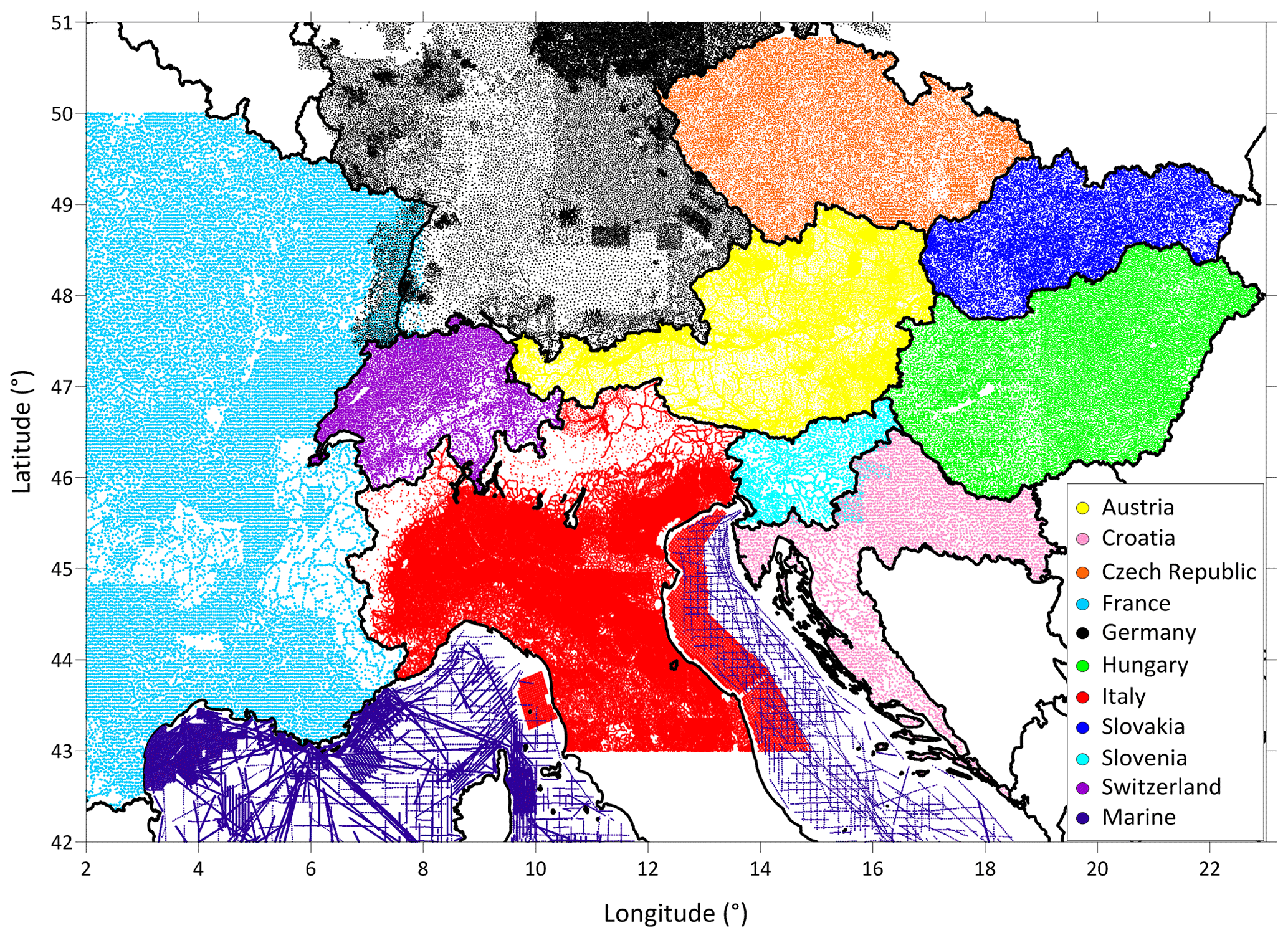
Figure 1The distribution of more than 1 million gravity stations in the area of investigation and compilation. Colors indicate the national databases used in the compilation.
2.1 Problems with positioning, heights and gravity data
One of the key problems in the unification of gravimetric databases is the homogenization of position, height and gravimetric coordinate systems used in each database. Through its historical development, each country has used and sometimes still uses local systems and their realization (frame), which are often based on the established principles of reference systems using older ellipsoids or older geodetic reference networks and projections. These systems and their realizations thus contain several differences which are responsible for large inhomogeneities, shifts and errors in position, height and gravity. These errors are most evident in the mutual comparison of data from individual countries.
To avoid these problems in the position of gravimetric points, all position data were transformed from local systems to the European Terrestrial Reference System 1989 (ETRS89), which is accurate, homogeneous and recommended for all European countries (Altamimi, 2018). A similar situation is in the height systems in that countries use different types of physical heights, they are linked to different tide gauges, and each country has a different practical implementation of the relevant height system. The solution is again the transformation to a uniform platform in the form of ellipsoidal heights in the ETRS89 system based on the ellipsoid GRS80 (Moritz, 2000). The situation is similar in gravimetric reference systems, in which especially the gravimetric databases that have been created for decades often use old gravimetric systems linked to the Potsdam system. An important step was therefore to convert these data into gravimetric systems which are connected to absolute gravimetric points and measurements, such as IGSN71 (Morelli et al., 1972) or modern national systems connected with the recent absolute measurements, which are verified by international comparisons of absolute gravimeters (Francis et al., 2015).
For these transformations, national transformation services were used (operated by national mapping services, e.g., SAPOS, SKPOS) or transformations implemented into standard GIS tools or our own software implementations based on national standards, information and experience of individual responsible institutions. The transformation from physical heights in national vertical systems to ellipsoidal heights in the ETRS89 system, ellipsoid GRS80, was realized using available local geoid and quasi-geoid models available through transformation services or implemented in current geodetic processing programs (e.g., Trimble Business Center, Leica Infinity). If a local geoid or quasi-geoid model was not available for some areas, then the global geopotential model EIGEN-6C4 (Förste et al., 2014) was used for transformation. This model was also used for marine data, for which the height of points was not given or had zero value.
Provided data include a local identifier, horizontal coordinates in the local coordinate systems (except France and Croatia), physical height, ellipsoidal coordinates in the ETRS89 system, ellipsoidal height above the GRS80 ellipsoid (except France, the Czech Republic and Slovenia) and the gravity value. For each parameter available metadata describing, for example, coordinate system (ellipsoid, EPSG code), transformation method or transformation service used, and local geoid and quasi-geoid were also collected.
Figure 2 shows the transformation scheme. For data sets for which all information was available, an independent transformation control check was performed between the local and global coordinate systems and between physical and ellipsoidal heights using available geodetic geoid and quasi-geoid models. Differences in position were in the majority of cases less than 1 m. All larger differences were individually investigated. A similar situation was for the heights, for which differences were generally less than 50 cm. These differences were mostly caused by different transformations, its practical software realization or local specifics of the data set.
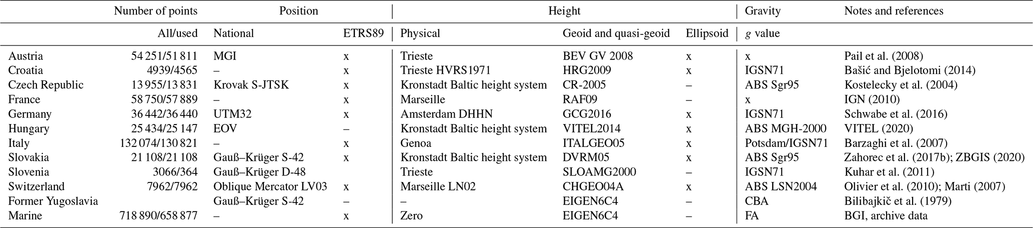
Data statistics and an overview of selected metadata are given in Table 1.
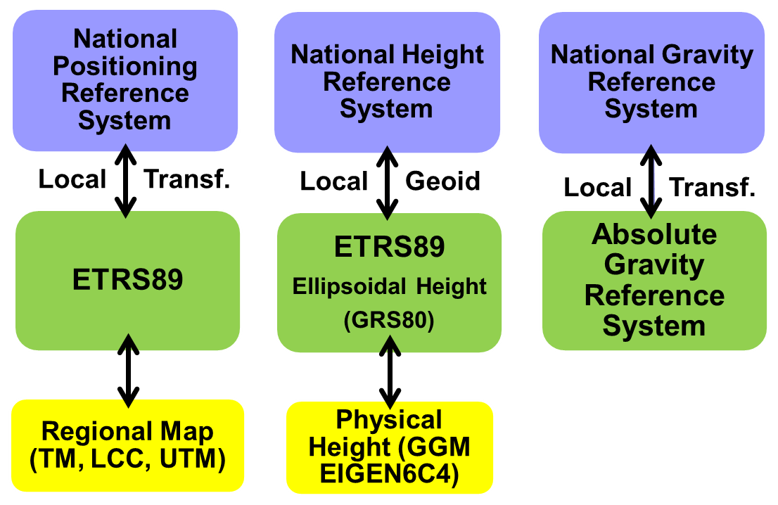
Figure 2Transformation scheme for unification of the national positioning, height and gravity reference systems.
Table 1Data statistics and an overview of selected metadata. From the total of originally 1 076 871 gravity stations, 1 008 815 data points were used for the compilation of the gravity maps. Most of the points were eliminated during the post-processing of offshore data.
2.2 Digital elevation models
One of the important elements in the calculation of complete Bouguer anomaly (CBA) is the calculation of proper mass corrections. The prerequisite for the calculation of correct gravity effects of topographic masses is the use of high-resolution digital terrain models (DTMs). Further information on the availability and use of DEMs in the Alpine area is given in Appendix C.
Both the new complete Bouguer anomaly (CBA) and the free-air anomaly of the studied region were calculated for ellipsoidal heights of calculation points with their geographical coordinates (λ, φ). For CBA mass corrections (gravitational effects of masses) δgM extending to the standard distance of 166.7 km, bathymetric corrections δgB and simplified atmospheric corrections δgA were applied. In contrast to the conventional processing of Bouguer gravity, a mass correction was calculated for masses between the ellipsoidal reference surface and the physical surface (Sect. 3.1). In addition, emphasis was put on the calculation of the gravimetric effects of the Alpine lakes on the basis of bathymetric data of the region (Sect. 3.2). To complete the AAGRG database an old CBA map from the former Socialist Federal Republic (SFR) of Yugoslavia (Bilibajkič et al., 1979) (Sect. 3.3) was digitized. Further improvements of the new CBA map are the refined calculations of an atmospheric correction and the future containment of distant terrain and bathymetry effects (Sect. 3.4).
The basic formula for the CBA calculation was adopted from Meurers et al. (2001):
where γ0(φ) results from the well-known Somigliana formula (Somigliana, 1929) for the normal gravity acceleration of a rotational ellipsoid at its surface (Heiskanen and Moritz, 1967):
and higher vertical derivatives of γ(φ, hE) are given by
All constants in Eqs. (3) to (5) were taken from the Geodetic Reference System 1980 (GRS80), e.g., in Moritz (1984):
-
γE=9.7803267715 m s−2, normal gravity acceleration at the Equator,
-
γP=9.8321863685 m s−2, normal gravity acceleration at pole,
-
a=6 378 137 m, semi-major axis of the normal ellipsoid,
-
c=6 356 752.3141 m, semi-minor axis of the normal ellipsoid,
-
f=0.00335281068118, geometrical flattening,
-
ω=7.292115 rad s−1, angular velocity of the Earth's rotation.
Simplified atmospheric corrections δgA (Wenzel, 1985) were calculated by means of the approximation
(δgA in mGal1, H in meters).
From a methodological viewpoint, the use of ellipsoidal heights for CBA calculation is innovative. Considering the participating countries, so far this concept has only been used in Austria (Meurers and Ruess, 2009). It ensures that Bouguer anomalies, which then, in the sense of physical geodesy, actually are gravity disturbances corrected for terrain mass effects, are not disturbed by the geophysical indirect effect (GIE; e.g. Li and Götze, 2001; Hackney and Featherstone, 2003) contrary to Bouguer anomalies relying on physical heights.
3.1 Mass correction
One of the main problems in the homogenization of data and recompilation of gravity fields was the use of different procedures for the calculation of mass correction (MC) and bathymetry correction (BC) by national operators/authorities. This meant that a complete recalculation had to be carried out for the new compilation based on the available point data and the best digital elevation models (DEMs) available. The proper choice of DEMs is discussed in Appendix C. An important first step before starting the recompilation was to test and select the available software to calculate the mass corrections. We compared two custom software packages developed by team members: Toposk software (Zahorec et al., 2017a) and TriTop (Holzrichter et al., 2019). Considering the results of this comparison (refer to Appendix D), we decided to use Toposk based on ellipsoidal heights hE of the calculation points and ellipsoidal digital elevation models (using in the majority of cases local geoids for the transformation). On the other hand, the bathymetric and simplified atmospheric corrections were calculated for physical heights H of the calculation points. Bathymetric corrections were also calculated by means of the Toposk software but in a slightly adjusted mode (see below and Fig. 3).
If the normal field in Eq. (1) is defined at the height above the surface ellipsoid, it is necessary to define the effects of terrain and bathymetry masses above the ellipsoid (not above the geoid). Therefore, the concept requires the use of ellipsoidal heights of the observation points, and at the same time it is necessary to transform the topography and bathymetry grids from physical to ellipsoidal heights. In the AlpArray area, the situation is more or less simple, the ellipsoid is below the geoid throughout the region (approx. 30 to 55 m). This greatly simplifies the calculation. In the case of continental areas, we get a slightly thicker layer of topography whose effect is calculated in the same way as in the case of physical heights (with the density of 2670 kg m−3). In the case of marine areas, the situation is somewhat more complicated as the ocean masses are partly above the ellipsoid level. If we want to take these into account with their real density (1030 kg m−3), it is necessary to separate their effect from terrain masses. Numerically, this can be done by taking these water masses into account first as topographic masses (i.e., with a density of 2670 kg m−3) and then also as part of the bathymetric correction (i.e., with a density of −1640 kg m−3). As a result, we assign a density ρ of 1030 kg m−3 to these water masses (ρ=2670–1640 kg m−3).
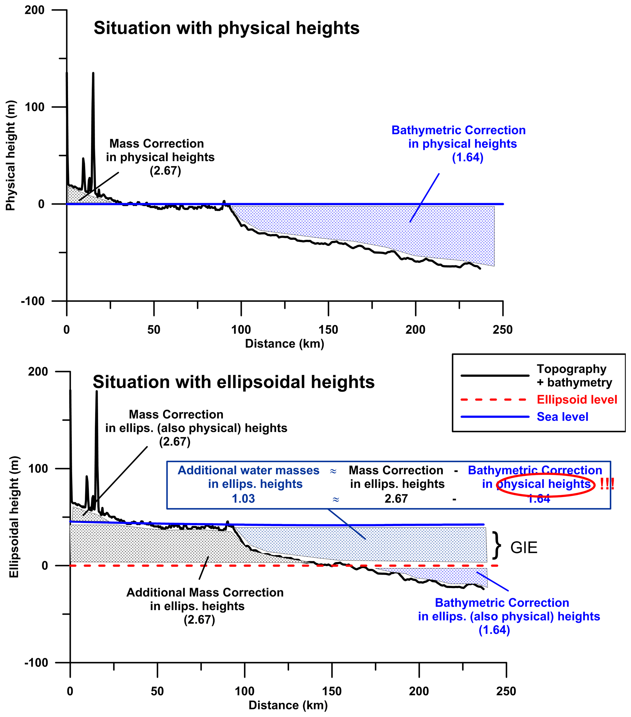
Figure 3Schematic comparison of physical vs. ellipsoidal concept of CBA. Note that the effect of additional water masses is calculated in a two-step process.
In connection with the above calculation methods, one note is appropriate. The difference between the two versions (physical vs. ellipsoidal heights) of the CBA defines GIE, which has a normal gravity component (defined by the free-air gradient) and a component defined by the gravitational attraction of the masses between the geoid and the ellipsoid. In our case, this second component is equal to the total gravitational effect of these masses with a density of 2670 kg m−3 (no difference in density at sea and on land). This is in apparent contradiction to published papers which state that the GIE should be calculated with different densities for land and sea (offshore with a density of 1030 kg m−3). This apparent discrepancy is due to different approaches to bathymetric correction. The approach of Chapman and Bodine (1979) is based on free-air anomalies which do not include bathymetric corrections, unlike our CBA. The GIE is thus easier to define in our case (for a constant density of 2670 kg m−3 in the whole space considered between the geoid and the ellipsoid) thanks to the consideration of the rock–water density contrast in this space as part of the bathymetric correction.
Figure 4 visualizes the MC values at all collected points. They reach values up to 375 mGal, while the ellipsoidal height of the points is from about 35 to 3938 m. The height dependence of the calculated MC is displayed in the lower right corner of the figure. The difference between the calculated MC and the gravitational effect of the truncated spherical layer (to the same distance) defines classic terrain corrections. They reach values of almost 100 mGal.
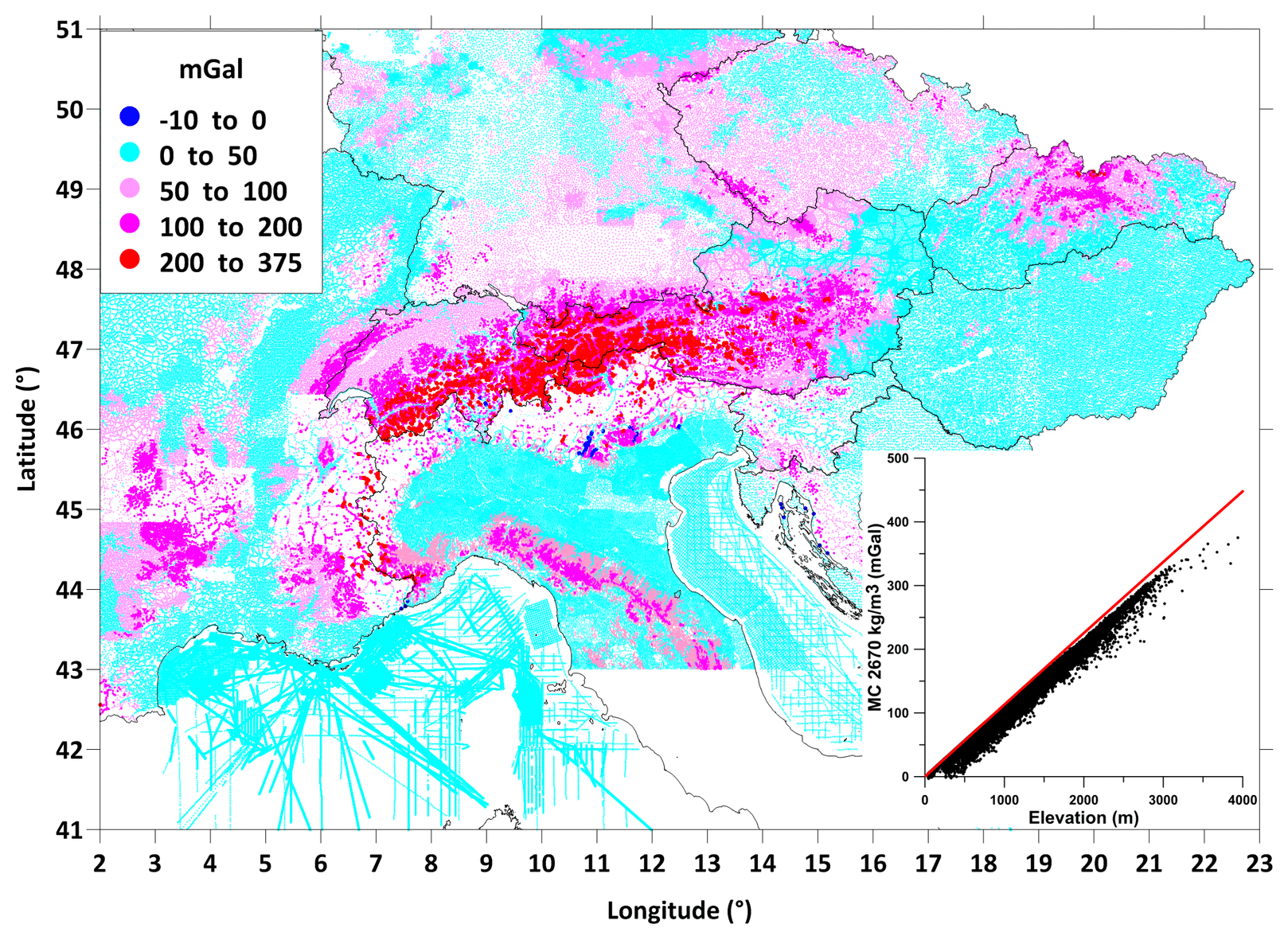
Figure 4Map of mass correction (up to the distance of 166 730 m, density 2670 kg m−3). Note the negative values of several milligals for a few points (dark blue points) which are mainly in deep valleys and near the coast. The graph in the bottom right corner shows the height dependence of the calculated MC. The red line represents the gravitational effect of the truncated spherical layer (up to the distance of 166.7 km, density 2670 kg m−3) for comparison.
3.2 Bathymetric and lake correction
3.2.1 Bathymetric corrections
When calculating bathymetric corrections (BCs), the gravity effect is calculated due to the difference in density between the water masses of the offshore areas and those of the land masses. In contrast to the MC, we calculate BC with physical heights as explained in Sect. 3.1 and Fig. 3. Water masses above the ellipsoid level are thus considered with their real density of 1030 kg m−3. We used a detailed bathymetric model EMODnet (EMODnet Bathymetry Consortium, 2018) with the resolution of 3.75 arcsec. A harmonized DEM has been generated for European offshore regions from selected bathymetric survey data sets, composite digital terrain models (DTMs) and satellite-derived bathymetry (SDB) data products, while gaps with no data coverage were completed by integrating the GEBCO digital bathymetry (GEBCO Compilation Group, 2020).
Bathymetric corrections reach significant values for offshore and near coastal points and amount to more than 200 mGal (Fig. 5). The comparison with the frequently used planar approximation is in the upper right corner of the figure. Unlike MC (refer to Fig. 4), these differences are not systematic and reach about ±30 mGal.
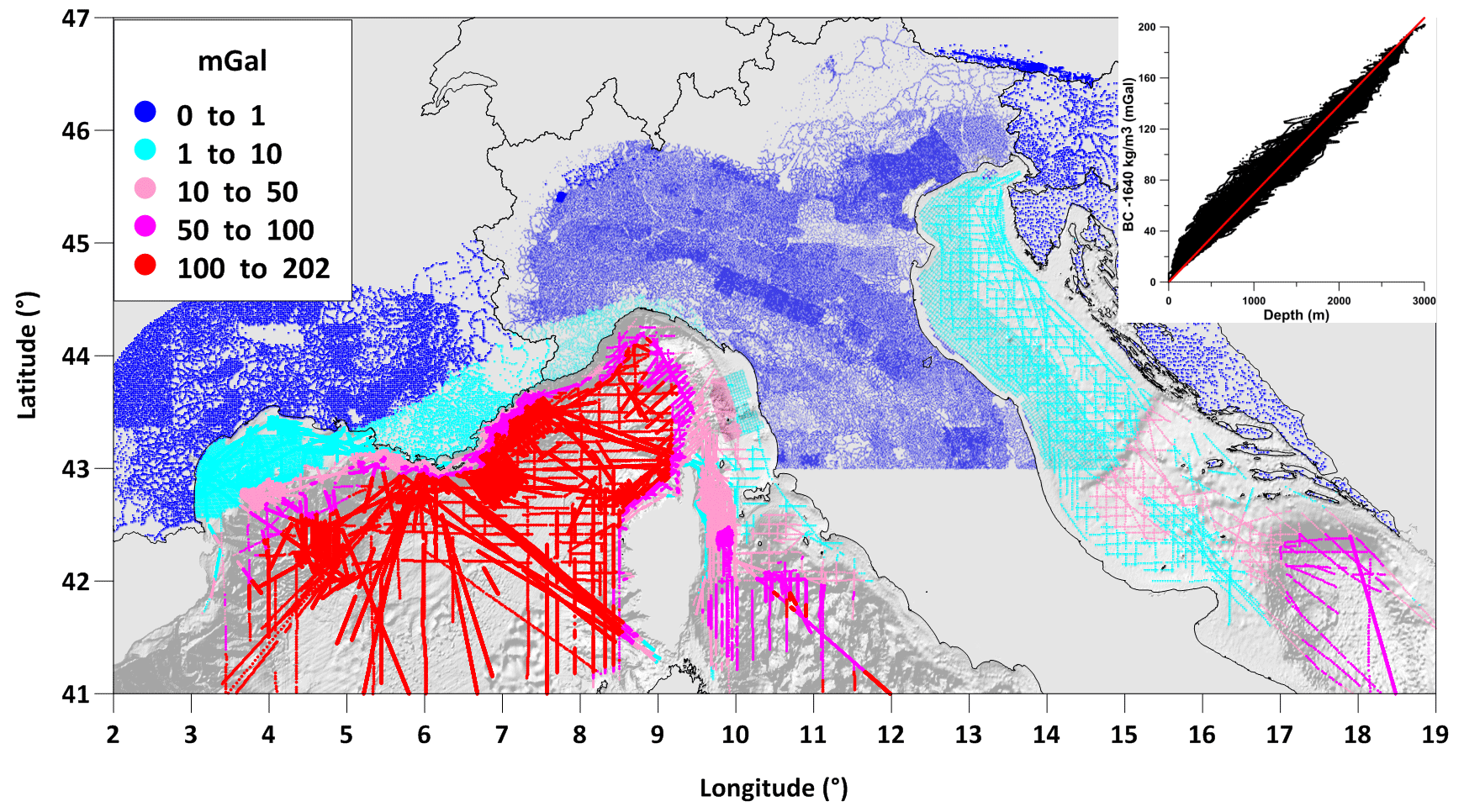
Figure 5Map of bathymetric corrections (up to the distance of 166.7 km, density 1640 kg m−3). Only non-zero values are shown on the map within 167 km of the sea. Shaded relief in the background shows the bathymetry of the seabed. The graph in the upper right corner shows the depth-dependence of bathymetric corrections. The red line represents their simple “Bouguer plate” approximation for comparison.
3.2.2 Lake corrections
Because the DEMs used in the MC calculation also include the volumes of water masses of Alpine lakes, these volumes are calculated with an incorrect density (2670 instead of 1000 kg m−3). We can eliminate this discrepancy by the application of a lake correction. Steinhauser et al. (1990) point out that some Alpine lakes reach a depth of up to 300 m and, due to easy accessibility, gravity stations are frequently located close to lake shores. An important prerequisite for a correct calculation is the availability of adequate models of lake bottoms. Except for Italy, depth models were available for four countries: for Switzerland, Austria, Germany and Slovenia.
For many large lakes in Switzerland bathymetric surveys have been carried out since 2007 (Urs Marti, personal communication, 2019). The resolution of these models varies between 1 and 3 m. For all the other lakes which contain bathymetric contours in the topographic map at a scale of 1:25 000, these contours have been digitized and interpolated to grids at a resolution of 25 m.
In Slovenia there are two big Alpine lakes of glacial origin located in the Julian Alps in the northwestern part of the country. For both lakes, high-resolution bathymetric data are available. Bathymetric surveys were performed in the years 2015–2017 (Harpha Sea, 2017). The maximum depths for Lake Bohinj and Lake Bled are 45 and 30 m, respectively. The bathymetric grid size of 20 m was used to compute the Alpine lake corrections for the new CBA.
No digital depth information was available for Austrian lakes. Therefore, shorelines and bathymetric contour lines have been digitized from topographic maps and interpolated to grids with 10 m spacing. All lakes (in total 36) exceeding either a water volume of 25 × 106 m3 or maximum depth of 50 m have been handled in this way, including artificial reservoirs. The altitude of the lake level surfaces was derived from topographic maps too. Seasonal lake level variations cannot be ruled out; however, they are expected to be less than 1–2 m for natural lakes. The situation may be worse for reservoirs.
The depth data for lakes in the German parts of the Northern Alps was digitized from topographic maps at a scale of 1:50 000. The resolution is 25 m or 1 arcsec. Vertical heights are physical (normal) heights.
The models mentioned were combined with existing detailed DEMs, and the lake correction itself was calculated as the difference of the gravitational effects of two topography models, one containing the level of the lakes and the other their bottom (e.g., Fig. 6 for Lake Geneva). Calculated lake corrections (density 1670 kg m−3) for all countries with available lake models are shown in Fig. 7. The corrections reach maximum values of about 5 mGal, especially on the lakesides with steep mountain flanks.
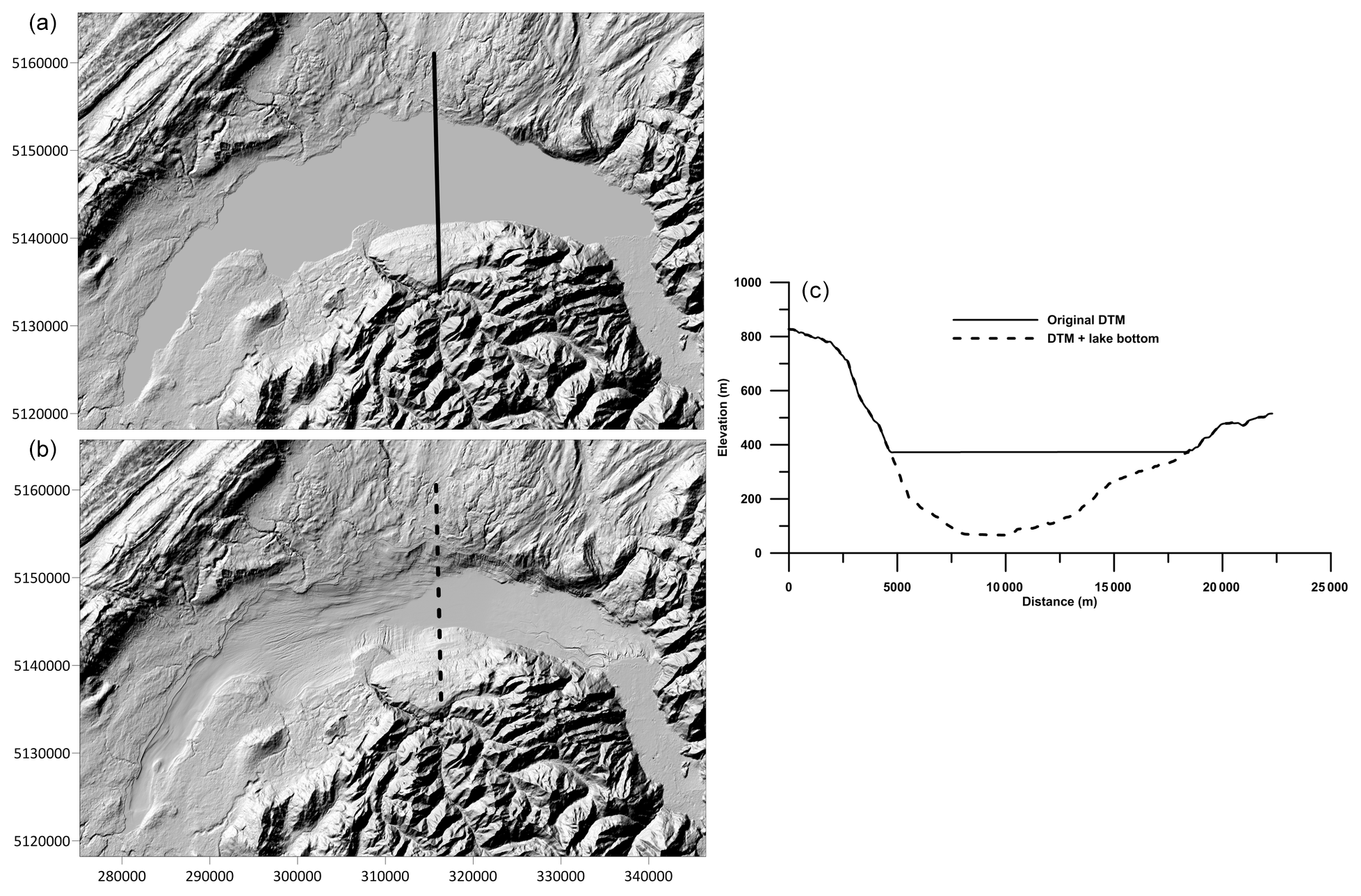
Figure 6Examples of topography models used to calculate lake corrections (here, Lake Geneva, Switzerland). Top shaded relief (a) represents the original DEM (MERIT) and the bottom one (b) the combination of DEM and lake bottom. The graph on the right (c) shows two profile lines crossing both models (north is to the right).
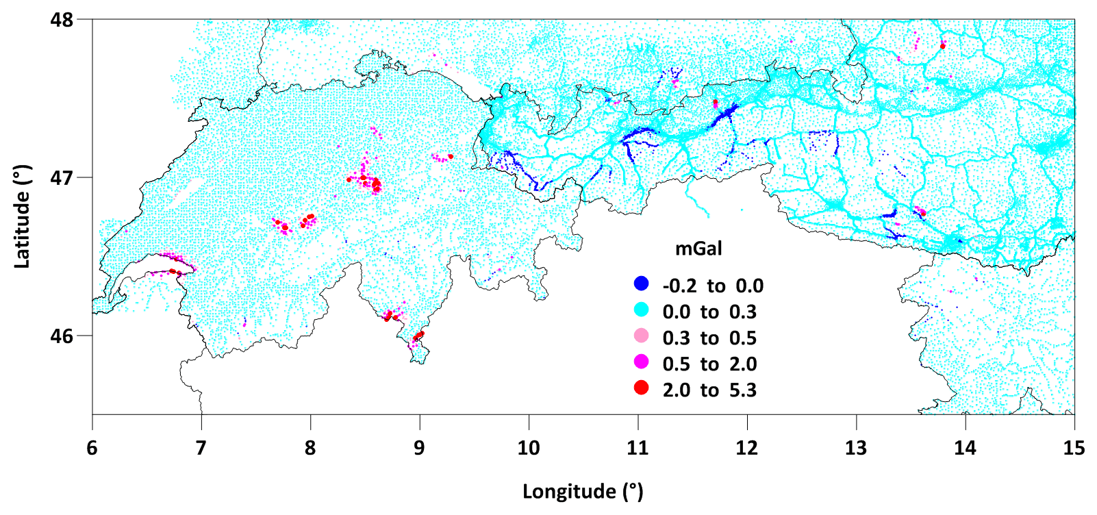
Figure 7Map of lake corrections (correction density is 1670 kg m−3). Small negative values occur in deep valleys with topography below the level of lakes (dark blue points). No corrections were calculated for the upper Italian lakes because no lake bottom information was available.
3.3 Digitization and reprocessing of the CBA map of the former SFR Yugoslavia
Although the peripheral southeastern part of the new Bouguer gravity map is not covered by terrestrial data which were available to the project, this area was filled by the digitization of the CBA map of the former SFR Yugoslavia at a scale of 1:500 000 (Bilibajkič et al., 1979). The CBA map (with a correction density of 2670 kg m−3) was published in 1972 and covers the whole area of the former SFR Yugoslavia. Its northern part was converted into an electronic form in the diploma thesis of Grand (2019). For the needs of the AlpArray project, a map was used especially for the territory of Serbia and Bosnia and Herzegovina. The gravity data of Slovenia and Croatia were also originally part of the Yugoslavian gravity map (refer to Appendix B – Croatia). In contrast to the digitization for the AAGRG described here, the Slovenian and Croatian database contains new data.
The reprocessing included the identification and correction of individual steps in the frame of CBA calculations to ensure a processing status which complies with that of the recalculated anomaly of the new AlpArray map. Specifically, normal gravity was corrected for the difference between the IGF 1967 and the Somigliana/GRS80 equations. Then the simple free-air correction was replaced by a more accurate approach, and the sphericity of the Earth was taken into account. However, this was neglected in cases when simple planar Bouguer corrections in the original data were used. For the last two corrections, the approximate heights at the digitization points generated from the model MERIT (multi-error-removed improved-terrain) were used. Finally, atmospheric correction was calculated, which was not considered in the original CBA. These reprocessing steps remained problematic as the uniform procedure of their calculation was not used for the original CBA map and the original values were not published. Therefore, given that MC and BC could not be recalculated and replaced by new values, we must expect more significant errors in the transformed CBA. Figure 8 shows a comparison of transformed CBA map with a map constructed from available data within the project for Croatia. Fortunately, the differences between the maps are not significantly large, the standard deviation of differences is about 1.8 mGal with a low systematic difference (the mean value of the differences is less than 0.5 mGal). We therefore assume that the replaced anomaly in the southeastern part of the map (Serbia, Bosnia and Herzegovina) is of similar quality than the main part.
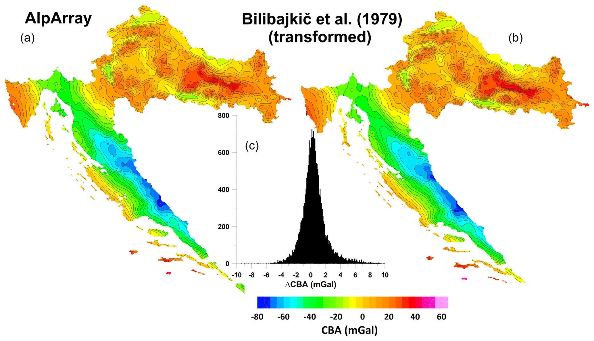
Figure 8Comparison of CBA maps (density 2670 kg m−3) for the area of Croatia. The map on the left (a) is constructed from available data within the AlpArray project. The map on the right (b) was obtained by transforming the digitized map of the former SFR Yugoslavia (Bilibajkič et al., 1979). The histogram in the middle (c) shows the differences between the maps.
3.4 A short remark on future treatment of true atmosphere and distant relief effects
As a challenge for the further development of the AlpArray CBA map, we also estimated the global effects of the true atmosphere and distant relief. Atmospheric correction is usually calculated based on a simple approximation according to Wenzel (1985). By the term true atmosphere, we mean the model of the atmosphere derived from the effect of a spherical shell with radially dependent density using the US standard atmosphere 1976 (Karcol, 2011) with an irregularly shaped bottom surface formed by the Earth's surface, calculated globally (Mikuška et al., 2008). The difference between atmospheric correction calculated by both approaches for the AlpArray region (calculated for selected database points) is shown in Fig. 9. The differences reach a maximum of about 0.16 mGal. As a function of height (approx. 0.04 mGal km−1) it mainly depends on the topography and to a much lesser extent also on the density model. Using a linear approximation instead of a time-consuming calculation at specific points would lead to maximum errors of about 0.02 mGal. Note that in order to maintain the real situation regarding the distribution of atmospheric masses, we used physical heights, not ellipsoidal heights.
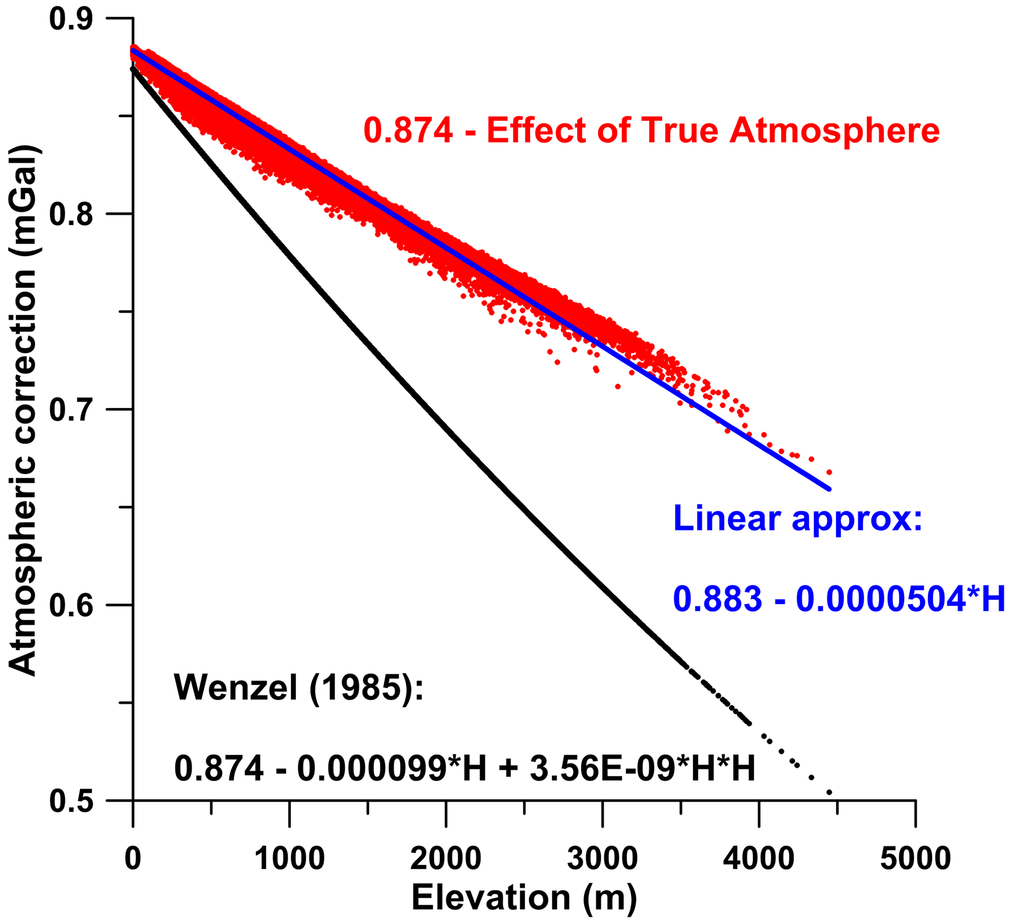
Figure 9Comparison of atmospheric correction at selected points covering the whole AlpArray area. The black dots represent the atmospheric correction calculated by a simple approximation according to Wenzel (1985). The red dots show the calculation using the effect of true atmosphere subtracted from the global constant value of 0.874 mGal (Mikuška et al., 2008), and the blue line is its linear approximation.
Distant relief effect (DRE) represents the combined effect of topography and bathymetry beyond a standard distance of 166.7 km around the whole Earth (refer to Mikuška et al., 2006, for more detailed information). Figure 10 shows this effect calculated at selected points in the AlpArray study area. The calculation was made in the classical concept of physical heights. The calculation for ellipsoidal heights would differ slightly (in quantitative terms), but the basic features would be retained as presented. The inclusion of this effect in the CBA is a task for future studies. DRE is dominated mainly by long-wavelength trends, superimposing also high-frequency patterns in mountainous regions due to its dependence on height. Because terrain masses are largely compensated for by isostatic compensation, distant-compensating mass distribution should be considered as well (e.g., Szwillus et al., 2016) either by applying isostatic concepts or by relying on global crust–mantle boundary models. However, these additional considerations are beyond the main objective of this publication.
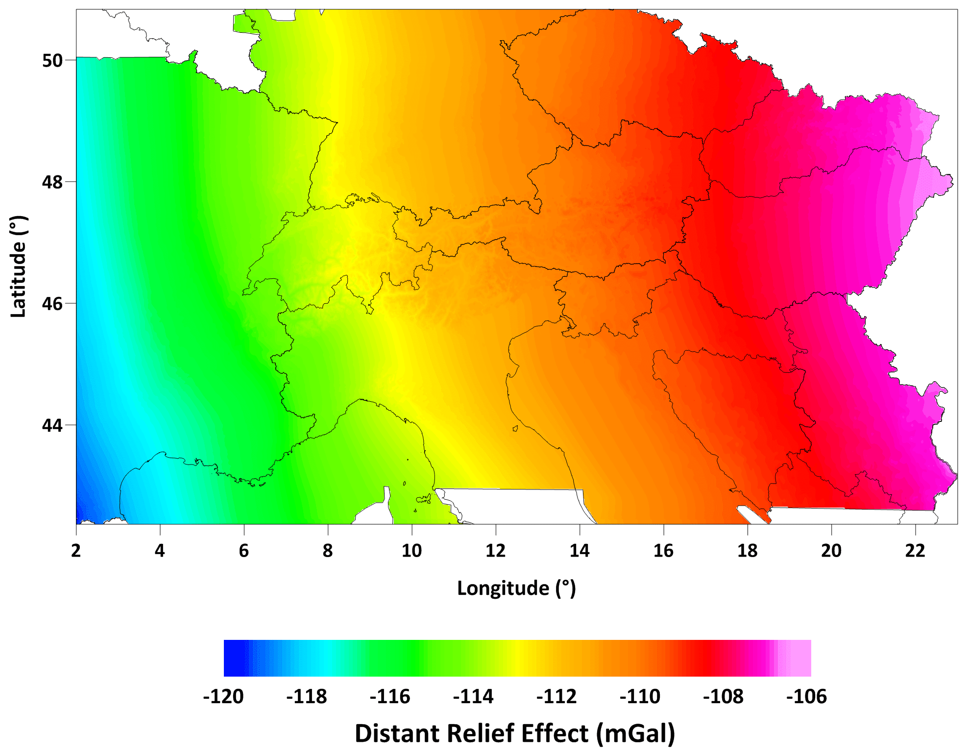
Figure 10The summary effect of topography and bathymetry (densities of 2670 and −1640 kg m−3, respectively) from 166.7 km around the whole Earth.
4.1 Interpolation and reference height of interpolated Bouguer anomalies
AlpArray gravity data have different levels of confidentiality. In some cases, only interpolated grids are available. Therefore, well-defined interpolation procedures are required. Interpolating scattered gravity data onto regular grids is commonly done in 2D, ignoring the fact that original data are acquired at different elevations rather than at a constant level. More exact solutions would be achieved by solving a proper boundary value problem. However, those methods are very time consuming, and avoiding mathematical artifacts due to limitation of data in terms of spatial extent and resolution is not trivial at all. Hence, the AAGRG decided to provide grids based on 2D interpolation first.
For assessing the 2D interpolation error in rugged terrain, two synthetic gravity data sets have been created based on two different kinds of source representation: a polyhedron model (method by Götze and Lahmeyer, 1988) and an equivalent source model (EQS) determined by the method of Cordell (1992). The model response has been calculated at the scattered positions of a subset of Austrian gravity data, as well as at the grid nodes with 1 km spacing. The synthetic data sets almost keep the wavelength content of real-world data. The elevation at the grid nodes was interpolated by 2D-Kriging based on the scattered data information.
In the case of the polyhedron model, the differences between exact 3D prediction and 2D interpolation do not exceed the range of 1–2 mGal. Only in small, isolated areas are the errors larger than 5 mGal. The same holds for the equivalent source representation in which the errors are in the range of ±1 mGal and exceed ±2 mGal only at a few spots (Fig. 11).
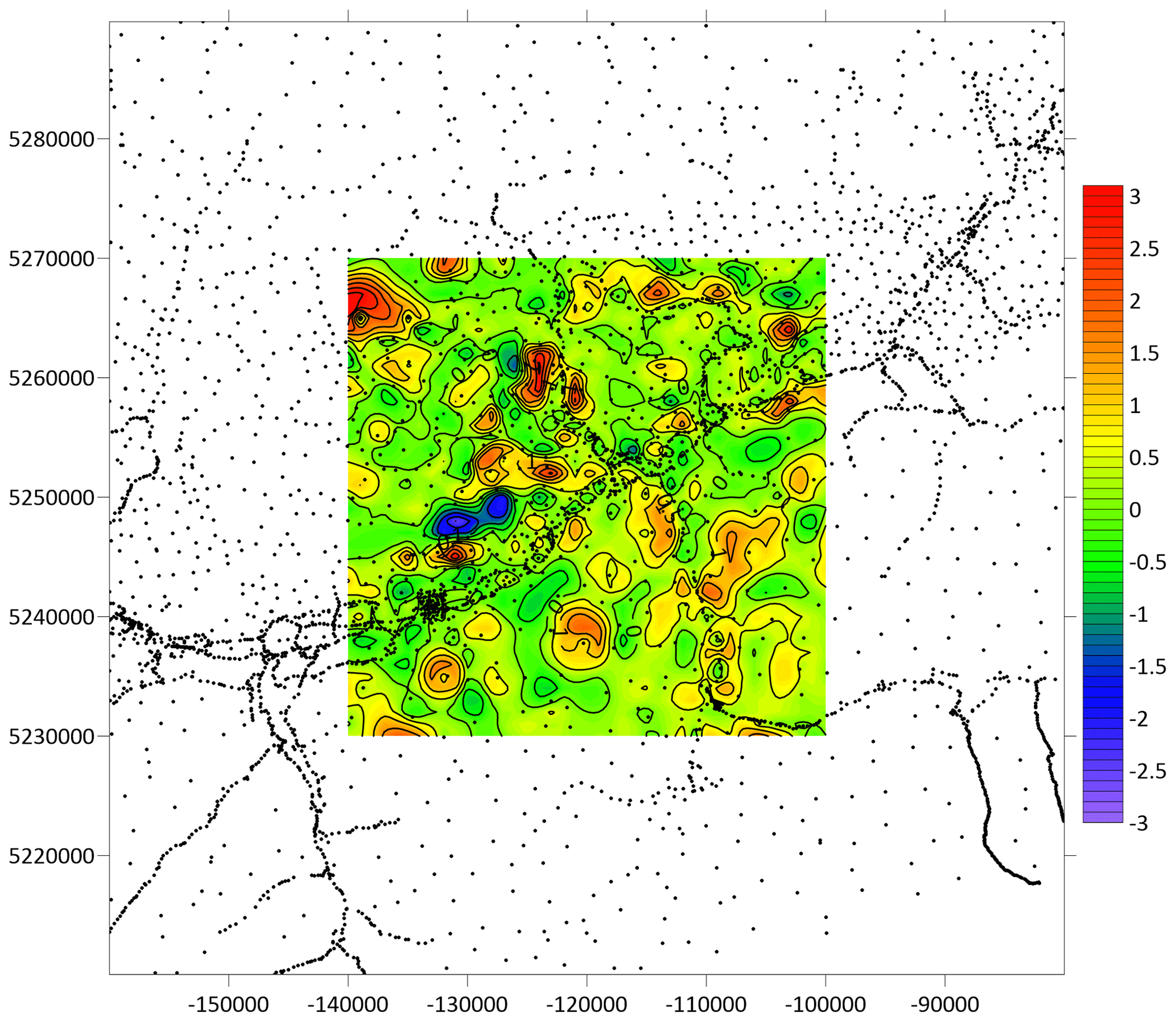
Figure 11Interpolation error estimate (gravity difference between gravity fields predicted by the EQS model and by 2D interpolation; contour interval 0.1 mGal, color bar in milligals (mGal) and axis coordinates in meters; Gauß–Krüger projection, M31).
In large-scale 3D modeling, 3D models rarely match the data better than the errors estimated in the scenarios tested above. Therefore, 2D interpolation seems to be justified even if it is not exact from a theoretical viewpoint. In local-scale interpretation, the situation may be different. However, another problem arises when using interpolated grids. Modelers need to know the elevation to which interpolated Bouguer or free-air anomalies refer.
Assuming the interpolation operator to be linear, Bouguer anomaly (BA) and free-air anomaly (FA) interpolated at each grid node (xi,yj) read as
where the suffix “int” denotes interpolated quantities and MC is the gravitational effect of surplus and deficit mass with respect to the reference ellipsoid. By transforming Eq. (7) and using Eq. (8) we get
Assuming the Bouguer anomaly to be a sufficiently smooth function of horizontal coordinates, true gravity at the position (xi,yj) of a grid node and at the true elevation htopo(xi,yj) can be approximated by
where the suffix “rec” denotes approximated (reconstructed) quantities.
The Bouguer anomaly at grid node (xi,yj) and at true elevation htopo(xi,yj) is
Approximating by Eq. (10) and inserting it into Eq. (11) results in
or
However, this approach neglects the fact that the Bouguer anomaly is the gravity effect of all sources at the true location of a station and therefore depends on the station heights as well. We would get the same result as in Eq. (12) for any arbitrary elevation h used in Eqs. (10) to (12), also for hint. Hence, we can interpret the interpolated Bouguer anomaly as being valid at the true elevation htopo(xi,yj) of a grid node (xi,yj) but also at elevation hint. Because interpolation is always associated with smoothing, we can argue that the best location for referencing the Bouguer anomaly is hint. If modelers use true elevations for the grid nodes, then models based on polyhedron approaches suffer from an aliasing problem because the topography is not well represented by the grid. A smoothed (interpolated) topography would work better because interpolation includes a kind of filtering.
Particularly in rugged terrain, FA and MC are not smooth functions of horizontal coordinates. Therefore, applying Eq. (9) is rather questionable. Instead, the free-air anomaly at a grid node (xi,yj) and at true elevation htopo(xi,yj) can be better approximated by
Inserting Eq. (7) into Eq. (13) results in
or with Eq. (8)
The free-air anomaly at the true elevation htopo(xi,yj) of a grid node (xi,yj) can be reconstructed either by Eq. (13) or (14). However, also in this case we have to keep in mind that we actually do not overcome the problem of the height dependence of Bouguer anomalies. When we use hint instead of htopo, Eqs. (13) and (14) hold accordingly.
Note that we implicitly also included bathymetry in the MC term appearing in Eqs. (7) to (14). Regarding the Bouguer anomaly BAρ calculated with density ρ differing from density ρ0 used in the mass correction (MC) term in Eqs. (7) to (14), we have to separate liquid from solid parts, which leads to the following equation:
where ρoc is the density of ocean water (1030 kg m−3).
Equation (15) neglects the small density difference between lake and ocean water. However, this leads to only small errors on the order of a few percent of the lake correction for reasonable crustal densities.
To conclude, in addition to the methodological procedures just described, we will now describe another problem related to the gridding of our database. In the case of the AAGRG compilation, interpolation of original and gridded data has been done by an iterative procedure:
- a.
Data providers, who were not allowed to release original information, created gridded data relying initially on their own scattered data and keeping only the nodes inside their own territory on a grid the AAGRG defined in common for the whole area.
- b.
After merging all data sets from AAGRG members one common grid was interpolated.
- c.
In the next step grid nodes of the neighboring countries were merged with the provider's original data set, and a new data grid was interpolated.
- d.
This iterative procedure continued until the variation of interpolated grid data close to the borders was well below an error threshold defined by ±1.5 mGal.
4.2 Filling data gaps using global geopotential models (GGMs)
We have focused on commonly used global geopotential models (GGMs) up to the degree/order of 2190, mainly on EIGEN-6C4 elaborated jointly by GFZ Potsdam and GRGS Toulouse (Förste et al., 2014) and EGM2008 (Pavlis et al., 2012). Both models are created by the combination of satellite and terrestrial gravity data. The spatial resolution of these models is roughly about 10 km.
The GGMs are usually used in connection with the so-called residual terrain modeling (RTM) technique, which greatly improves gravity values calculated from GGMs on the Earth's surface. The RTM technique accounts for the difference between the gravitational effect of the real terrain masses represented by high-resolution DEMs and smoothed mean elevation surface represented, e.g., by the DTM2006 model (Pavlis et al., 2007). However, since the effect of the detailed DEM would be subtracted retrospectively in the Bouguer anomaly calculation, it means that, in order to obtain BA, we only need to subtract the gravity effect of the DTM2006 (δgDTM2006(λ, φ, hE)) directly from the free-air anomaly calculated from GGM-derived gravity by the standard procedure of Eq. (16). Compared to Eq. (1), Eq. (16) lacks the term for the atmospheric correction because it is already included in the GGM:
where gGGM is the gravity calculated from a particular GGM at the Earth's surface (to be directly comparable with the terrestrial data) at elevations derived from the MERIT model, γ is the normal gravity, and δgDTM2006 is the gravitational (terrain and bathymetry) effect related to the model DTM2006 (of the corresponding degree of 2190) up to the distance of 166.7 km. The DTM2006 model was selected due to its close relationship with the creation of the model EGM2008. This model was originally compiled in a grid of 30 arcsec × 30 arcsec. For the purposes of our calculations, the model was transformed and resampled into a format corresponding to the calculation of the standard mass/bathymetric correction using Toposk.
We calculated the gravity values gGGM using the software GrafLab (Bucha and Janák, 2013) using the maximum degree of spherical harmonic coefficients for a specific GGM. Calculations were performed in GRS80 ellipsoidal coordinates.
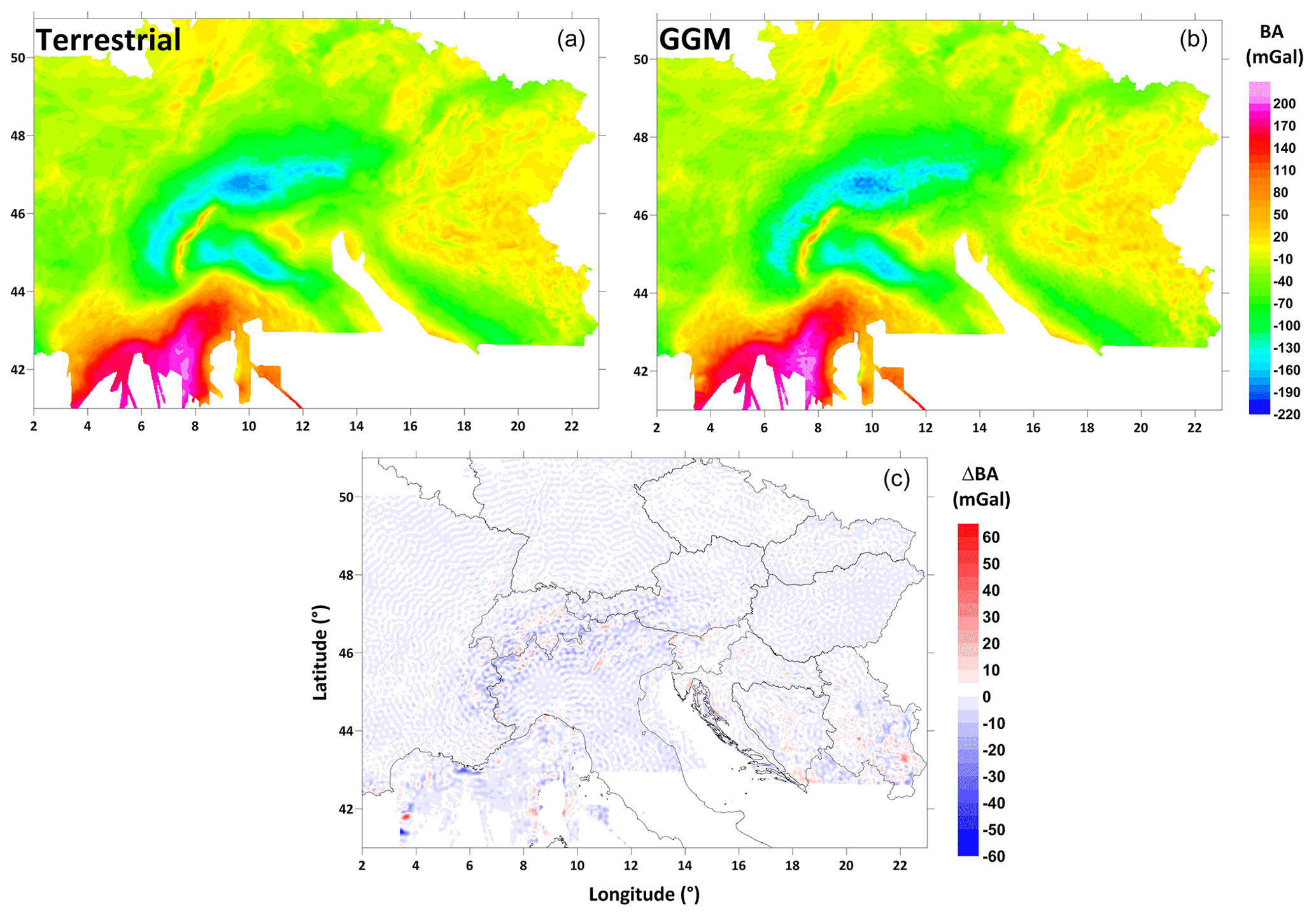
Figure 12Comparison of Bouguer anomaly maps (correction density 2670 kg m−3) derived from terrestrial data (a) and GGM EIGEN-6C4 (b). The bottom map (c) shows the difference between the two.
Figure 12 shows a comparison of a BA map derived from terrestrial data with the map derived from the EIGEN-6C4 model (calculation points were made on a 2 km × 2 km grid) in the area covered by terrestrial data. The maximum differences between grids are at the level of tens of milligals (RMS error is about 4 mGal) but without any systematic error. It follows that the GGM-derived map can be used to fill in gaps (marginal parts) in the terrestrial data.
GGM data points located in gaps of the original gravity points were separated by the shortest distance criteria of 15 km using a standard database search query in QGIS. A 15 km criterion was chosen as a compromise between covering GGM data close enough to the vicinity of the terrestrial data (Fig. 19) but at the same time not filling gaps that are too small between them, which could lead to local artificial anomalies.
4.3 Brief interpretation of Bouguer anomaly map
We here present a short overview of the features of the new Bouguer anomaly map (Fig. 13). The most prominent feature of the complete Bouguer anomaly (CBA) is the Alpine gravity low (AGL), which is characterized by gravity values ranging from −100 to −170 mGal. The AGL corresponds with the Alpine mountain chain and is explained by the isostatic crustal thickening, as demonstrated by the good anticorrelation with topography (Braitenberg et al., 2013; Pivetta and Braitenberg, 2020) and the isostatic compensation and gravity forward models (e.g., Ebbing et al., 2006; Braitenberg et al., 2002). It could be divided into local gravity lows that correlate with the Western, Central and Eastern Alps. Among all of them the Central Alps (the easternmost part of Switzerland) are accompanied by the highest amplitude: −170 mGal.
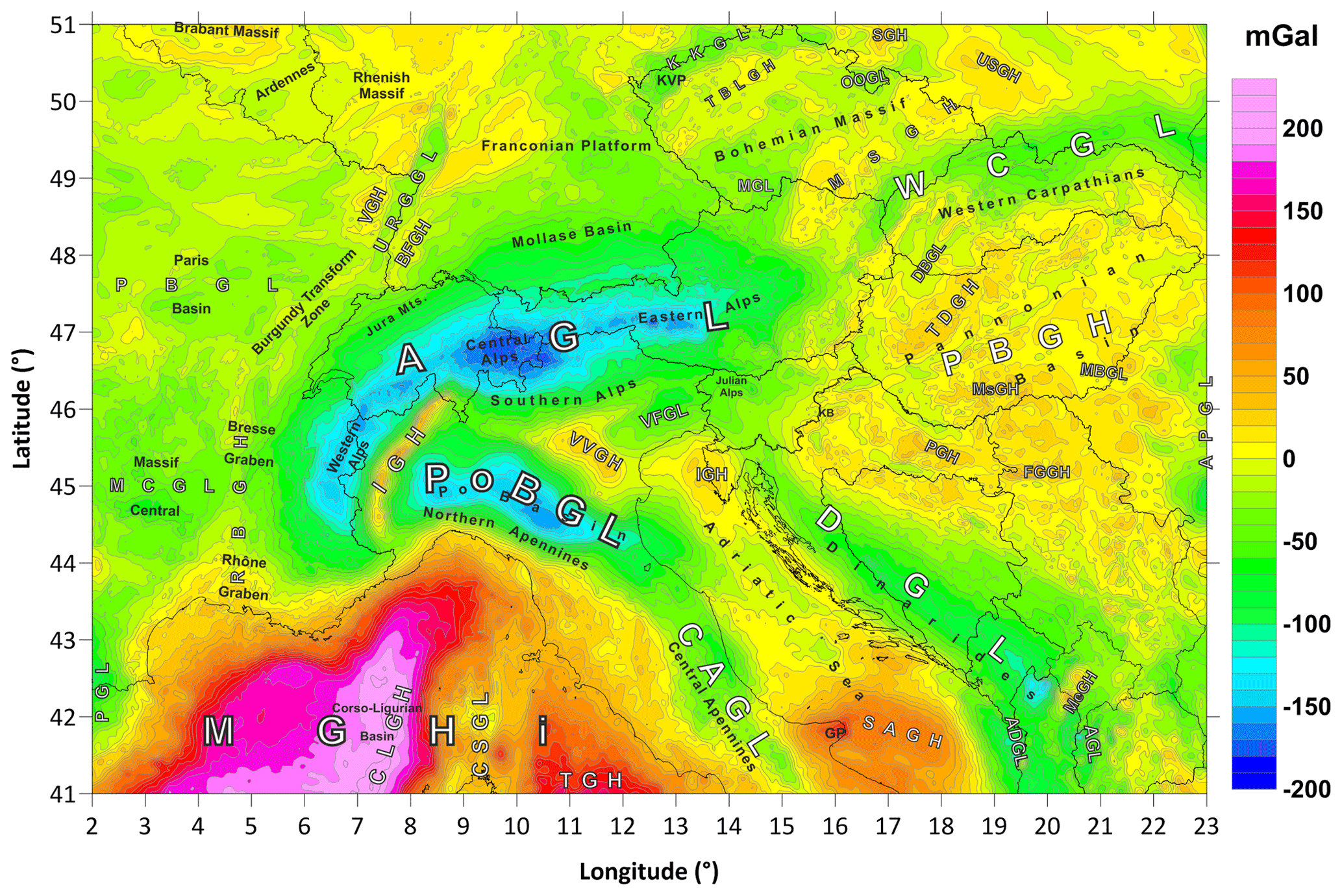
Figure 13New pan-Alpine Bouguer gravity anomaly map. The first order dominant regional gravity anomalies: AGL – Alpine gravity low, PoBGL – Po Basin gravity low, CAGL – the Central Apennine gravity low, IGH – Ivrea gravity high, VVGH – Verona/Vicenza gravity high, VFGL – Venetian/Friuli Plain gravity low. The second dominant regional gravity anomaly: MGHi – Mediterranean gravity high, CLGH – Corso/Ligurian gravity high, TGH – Tyrrhenian gravity high, CSGL – Corsica/Sardinia gravity low, SAGH – south Adriatic gravity high, IGH – Istria gravity high, WCGL – Western Carpathian gravity low, DGL – Dinaric gravity low, MeGH – Merdita gravity high, ADGL – pre-Adriatic depression, PBGH – Pannonian Basin gravity high, TDGH – Transdanubian gravity high, PGH – Papuk gravity high, MsGH – Mecsek gravity high, FGGH – Fruška Gora gravity high, DBGL – Danube Basin gravity low, MBGL – Makó/Békés Basin gravity low, APGL – Apuseni gravity low. The rest of the study area: PGL – Pyrenean gravity low, MCGL – Massif Central gravity low, PBGL – Paris Basin gravity low, URGGL – Upper Rhine graben gravity low, RBGH – Rhône/Bresse Graben gravity high, BFGH – Black Forest gravity high, VGH – Vosgesian gravity high, KKGL – Krušné hory (Erzgebirge)/Krkonoše gravity low, TBLGH – Tepla/Barrandian/Labe gravity high, MGL – Moldanubic gravity low, OOGL – Orlice/Opole gravity low, MSGH – Moravo/Silesian gravity high, USGH – Upper Silesian gravity high, SGH – Sudetes gravity high, KB – Krško Basin. A high resolution 600 dpi plot of the map is available in the supplement.
A second prominent low is the Po Basin gravity low (PoBGL). The gravity values here range from about −80 to −140 mGal. The PoBGL continues in the southeastern direction to the Central Apennine gravity low (CAGL), whose amplitude (−40 mGal) is significantly smaller in comparison with the Northern Apennine gravity low. In the southeasternmost part of the Central Apennines the CAGL thins out gradually.
A significant anomaly feature represented by a very narrow local gravity high can be clearly recognized between the Western Alps and the Po Basin. This anomaly is well known as the Ivrea gravity high (IGH). It is characterized by maximum values of +40 mGal caused by dense, lower crustal and mantle rocks that are exposed and in the near subsurface and that are planned to be drilled in the forthcoming DIVE project (Pistone et al., 2017; http://dive.icdp-online.org/, last access: 15 May 2021). It is important to note that its relative amplitude compared to the gravity lows in the Western Alps and the Po Basin reaches up to 160 mGal. It is the highest horizontal gravity gradient in the study region.
To the northeast of the Po Basin, we can observe the Verona/Vicenza gravity high (VVGH), which has been recently modeled as being generated by increased density crustal intrusions related to the Venetian magmatic province (Tadiello and Braitenberg, 2021; Ebbing et al., 2006). The Venetian/Friuli Plain gravity low (VFGL) is located in eastern Italy, which is presumably caused by low-density sedimentary infill, also like the gravity low in the Po Basin (Braitenberg et al., 2013).
A prominent gravity high is the Mediterranean gravity high (MGHi). This regional-scale anomaly has its maximum over the Corso/Ligurian Basin, the Corso/Ligurian gravity high (CLGH). It is characterized by maximum values of +200 mGal. The regional MGHi also includes the Tyrrhenian gravity high (TGH). The study covers only the northern part. Gravity values do not exceed +140 mGal. The Corso/Ligurian gravity high and the Tyrrhenian gravity high are separated from the relative Corsica/Sardinia gravity low (CSGL). The values vary from +20 to +60 mGal.
The Adriatic Sea region is largely characterized by a positive gravity field, in which the south Adriatic gravity high (SAGH) dominates with values from +20 to +100 mGal. Its maximum is located over the Gargano promontory. In the northwestern part of the Adriatic Sea, negative gravity values up to −80 mGal are observed, which belong to the easternmost part of the Po Basin gravity low. West of the Istrian peninsula the center of the residual Istria gravity high (IGH) is present, with maximum values of +30 mGal.
In the Eastern Alps, the AGL splits towards the east into two branches of less pronounced gravity lows: the Western Carpathian gravity low (WCGL) and the Dinaric gravity low (DGL). In the Western Carpathians, the values vary from 0 to −60 mGal, while the Dinaric values range from 0 to −120 mGal (Bielik et al., 2006). The lower amplitude of the gravity field of both the WCGL and the DGL in comparison with the AGL most likely reflects a weaker continental collision resulting in thinner crust under the Carpathians and Dinarides. In the Adriatic region we can also recognize the Merdita gravity high (MeGH) and the pre-Adriatic gravity low (ADGL).
The Pannonian Basin extending between the Western Carpathians and the Dinarides is accompanied by a relatively regional gravity high (Pannonian Basin gravity high, PBGH) whose values range in a narrow interval from −10 to +20 mGal. The PBGH consists of several local positive (the Transdanubian gravity high, TDGH, the Papuk gravity high, PGH, the Mecsek gravity high, MsGH, the Fruška Gora gravity high, FGGH) and negative anomalies (the Danube Basin gravity low, DBGL, the Makó-Békés Basin gravity low, MBGL). The gravity effect of the Apuseni Mountains is negative (as low as −80 mGal).
The rest of the study area extending north of the MGHi, AGL and WCGL is accompanied by an indistinct yet variable gravity field with the values varying generally from −80 to +40 mGal. Based on the analysis of the gravity field in this area, we recognize the following anomalies: the Pyrenean gravity low (PGL), the Massif Central gravity low (MCGL), the Paris Basin gravity low (PBGL), the Upper Rhine graben gravity low (URGGL), the Rhône/Bresse Graben gravity high (RBGH), the Black Forest gravity high (BFGH) and the Vosgesian gravity high (VGH).
The gravity field of the Bohemian Massif can be divided into several subparallel positive (up to +20 mGal) and negative (0 to −60 mGal) belts with predominantly northeast–southwest orientation: the Krušné hory (Erzgebirge)/Krkonoše gravity low (KKGL), the Teplá/Barrandian/Labe gravity high (TBLGH), the Moldanubian gravity low (MGL), the Orlice/Opole gravity low (OOGL), the Moravo/Silesian gravity high (MSGH), the Upper Silesian gravity high (USGH) and the Sudetes gravity high (SGH).
The gravity field over the Franconian Platform area north of the Molasse Basin is quite variable, and values range from −40 to +15 mGal. The eastern part of the Franconian Platform is characterized predominantly by negative values, while the western part is characterized by positive values.
The Rhenish Massif is distinctly asymmetric, positive (up to approx. +20 mGal) over the eastern massif and negative (to approx. −20 mGal) over the western massif. The Ardennes are accompanied by the gravity low of −20 mGal. The Brabant Massif is manifested by a gravity high with an amplitude of +20 mGal.
The newly compiled gravity database of the Alps and their surroundings is based on decades of data collection and processing experience of the AAGRG members. The national gravity data, which were recompiled here under new, modern geophysical and geodetic aspects (Sects. 2 and 3), were collected with rather different instruments at different times over the last 70 years and processed with extremely different processing methods. At the end of the data processing, we therefore asked ourselves for what purposes it can be used and how accurate the new map actually is. The first question can be answered relatively easily: with medium- to large-scale modeling of the Alpine lithosphere and/or the Alpine Earth crust, as realized in the AlpArray initiative, there should be no problems with the final accuracy of the database: these errors are small compared to the uncertainties that result from modeling and simulation. The second question about accuracy (uncertainty), which is caused by using extremely different data sets, is much more difficult to answer because in practice for all participating countries there are no exploitable metadata available for the national gravity databases.
As desirable as it would have been for the submitted pan-Alpine gravity maps to present “uncertainty maps” at the same scale, this project is hindered due to the complexity of the task and the lack of information on errors and accuracies in the field campaigns and data processing of the individual countries. However, in order to obtain an estimate of the uncertainty, we have tried in the following section to list various aspects of error analysis by way of examples. It must be reserved for a later publication to present a numerical-statistical analysis of the map (e.g., with the time consuming sequential Gaußian simulation; e.g., Shahrokh et al., 2015) or statistical evaluation compared to the GOCE (Gravity field and steady-state Ocean Circulation Explorer) gravity observations that have lower spatial resolution but homogeneous error (Bomfim et al., 2013).
5.1 Testing at independent gravity points – example from Slovakia
In Fig. 14 we show a test calculation that demonstrates the differences between the fields of the interpolated CBA and point stations in Slovakia. These “test data” have not been considered for the interpolation of the Slovakian gravity grid – thus they represent an independent test of the map quality. First, it should be noted that no deviations are greater than ±5 mGal. The mean is 6 µGal and the standard deviation is 0.88 mGal. This is an ideal example for visualizing “mapping errors” which are expected in the case of a dense and widely homogeneous data coverage. However, in areas of less dense and less homogeneous coverage like along the Alpine crests or in the offshore areas, the number of errors increases.
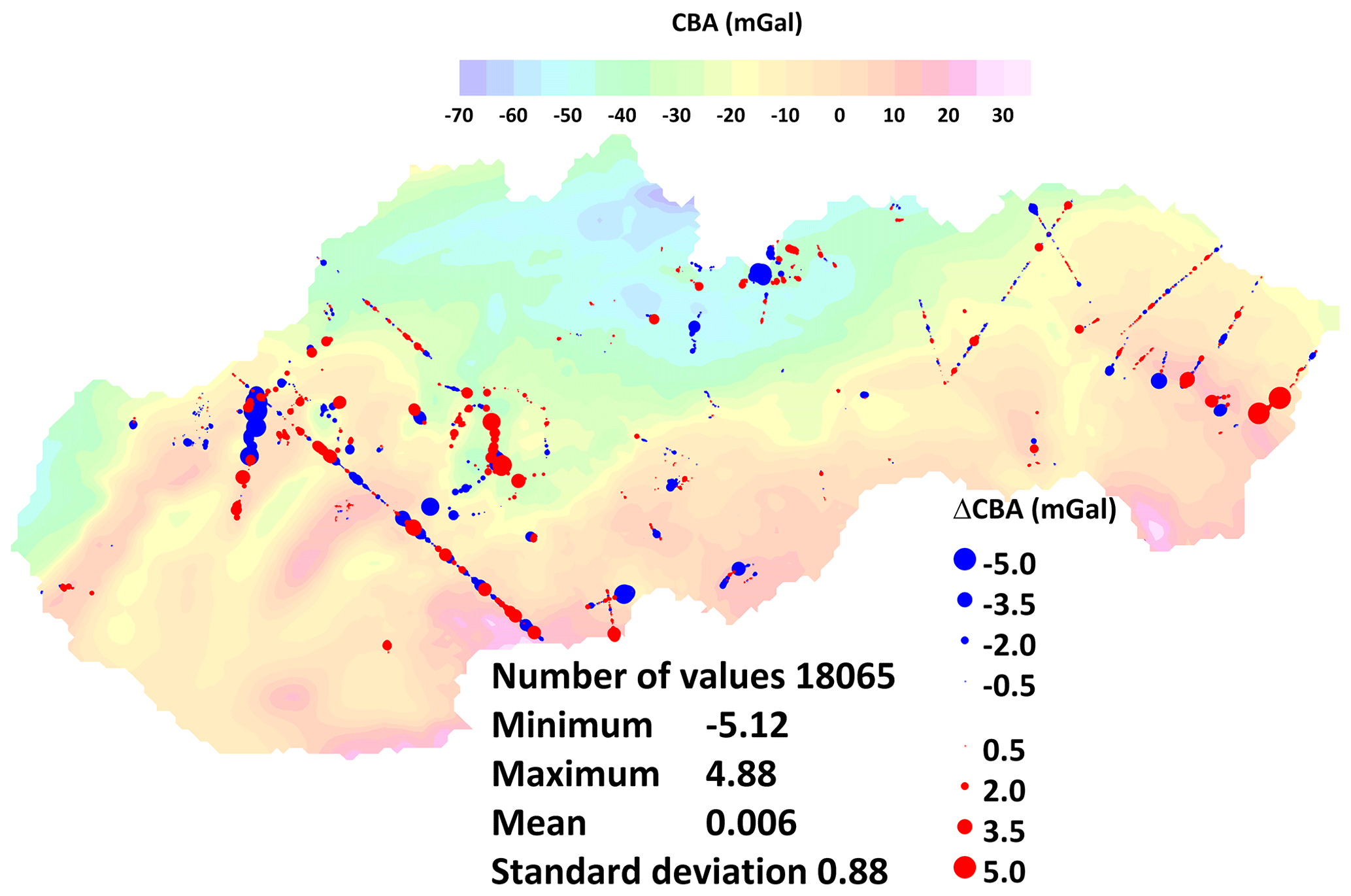
Figure 14Differences between the CBA grid and independent gravity points (not used for the Slovakian part of the gravity grid compilation). It was calculated by SURFER's simple grid-residual procedure and showed that no gravity differences were greater than ±5 mGal.
5.2 Possible sources of errors
The sources of errors in gravimetric measurements are manifold and result directly from the definition of the Bouguer anomaly and the processing of associated reduction and correction terms (Sect. 3, Eq. 1). Instrumental readings in gravimetry depend on the instrument drift and the accuracy of the scale values and are of course dependent on the external conditions in the field. In addition, there is a correction of the Earth's tides and the air pressure. The localization of the station with longitude, latitude and altitude, as well as its geographical context (e.g., measured along profiles, areal measurements, located in valleys with extensive sedimentary filling, etc.), is also subject to errors. The density of the station distribution (Fig. 1) certainly has a great influence on the accuracy of the resulting maps. This is, however, good enough for the above-mentioned modeling of the lithosphere – very small-scale modeling on a kilometer scale is excluded.
Even the indication of the positional accuracy of the gravity stations and the DEMs used pose great problems, and most of the information is not available in digital formats. The same is true for the above-mentioned field instruments and procedures used, which have been improved often over the last 70 years, and of course for the processing techniques, which started with manual-graphic methods and still allow for digitized processing from field measurements to 3D interpretation (among many others: Cattin et al., 2015; Sabine Schmidt, personal communication, 2019).
Furthermore, different numerical approaches that can be used for the data processing provide different results. In Appendix D we reported test investigations which led to the selection of the software for the calculation of the MC (Appendix D, Fig. D1). A comparison of the standard deviations (1.95 mGal for the software TriTop and 0.39 mGal for Toposk) also gives an indication of the achieved accuracy of the database – even if this can only be a partial aspect.
Two other sources of error deserve a closer look. In Sect. 5.2 we will discuss errors that occur when calculating the mass correction with different correction densities. Notes on the accuracy of the anomalies due to a 2D (on the map projection plane) and a 3D interpolation needed have already been given in Sect. 4.1. Based on national investigations in the area of Austria, indications of the achieved numerical accuracy of the Bouguer anomalies are then given in Sect. 5.3. Finally, in Sect. 5.4 the results of an error statistic based on cross validations (CVs) are given for the entire database.
However, it should not be forgotten that CV is a purely statistical measure and in minor amounts considers point data quality, which indicates that we cannot directly represent the quality of the newly compiled gravity fields from the CV.
CV works well with dense station coverage; only then can we exclude large local anomalies, for example, due to geological causes. The less dense the coverage is, the less we can exclude the presence of local anomalies. Note that these local anomalies can easily be produced by selecting improper MC density, for example, in a station setting covering a valley and adjacent mountain flanks where densities differ from the assumed MC density remarkably.
5.3 Errors in the calculation of mass corrections (MC)
The DEM used has a significant influence on the result. For example, differences in MC calculations using the lidar and MERIT DEM (Appendix D, Fig. D4) resulted in values of ±5 mGal. In addition to the errors arising from the use of inexact models of the topography, additional errors can result from the varying density distribution of the masses outside the reference ellipsoid. According to Eq. (1), the Bouguer anomaly has an exact physical meaning (Meurers, 2017): it is the integral gravity effect of all sources which differ in density from (a) the rock densities outside the ellipsoid as used in the MC and from (b) the density inside the reference ellipsoid. Three cases will be discussed in more detail here, according to their significance.
5.3.1 The normal case (A)
Consider that the calculation of MC is already part of the modeling which has to be performed with the best possible spatial resolution. For this, the density of the masses is constant. If this density corresponds to the real density, then only volumes of a different density within the ellipsoid must be recognized as additional sources. For any later modeling, this setup simplifies the model geometry considerably. If, however, the constant MC density differs from the natural conditions, these masses must be addressed with a different density in the model, resulting in substantially more complicated geometry. In addition, these model masses must be calculated with the same spatial resolution as used in the calculation of the MC. If one considers that resolutions of the topography of 10 m × 10 m are common for local gravity investigations, this has consequences for the handling of the model. It must then also be designed with a correspondingly high resolution, and it becomes no longer easy to handle because of its size. Theoretically, this is feasible, but it is not practical due to computational reasons. Therefore, in practice, smoothed topography models are commonly used to keep the number of parameters under control. From the spatial deviations of smoothed and high-resolution topography, deviations between the measured and modeled field can arise.
5.3.2 The 2D case (B)
Here, essentially the same applies as in the normal case (A) except that the creation of the initial model is considerably more complicated. A 2D density model is used for the MC and, hence, must be considered in successive models. As the same statement as above can be made, this complicates the model setup compared to the normal case (A). However, the 2D case makes sense if it is to be used for qualitative interpretation since the 2D model represents the natural conditions much better than when using a constant MC density.
5.3.3 Knowledge of the real density distribution (C)
Unfortunately, this case is only applicable in theory as the real density distribution is always characterized by MC densities which are not constant and not known for data processing or modeling. A priori knowledge would be the optimal case, but in this case, 3D modeling and the MC correction for the BA have to be done simultaneously in an integrated modeling framework. In order to interpret and model gravity anomalies quantitatively, it is recommended to choose the normal case (A).
The consequences for possible errors for MC from the three cases are as follows. If we would regard incorrect MC density as an error source, these errors can be as high as 700 kg m−3 (e.g., in valleys). Then, the MC error results from multiplying the density errors by the MC calculated with unit density and is likely of the order of 30–50 mGal or higher, which is about 10 %–20 % of the BA of the Alps.
When including the actual density errors in the error balance, we would observe large errors of 50 mGal and more. Using these errors as a criterion for the quality of fit in the 3D model calculation makes no sense. However, if we take the physical interpretation of the BA (as explained at the beginning) as a baseline, MC density errors are indeed not errors but objects of the model calculation.
5.4 Mapping errors in selected areas of the map
As already discussed in Sect. 4.1, any 2D interpolation procedures for Bouguer values are not exact. However, for large-scale interpretation these errors are negligible. Instead, we use two approaches for assessing the interpolation error: interpolation residuals and cross-validation residuals. Interpolation residuals depend on the mathematical representation of the interpolation grid. We use the bilinear interpolation method for calculating the residuals at points that do not coincide with grid nodes. Interpolation residuals describe how exact the scattered data are represented by the interpolation surface. Cross-validation residuals are calculated by removing one observed station from the data set and using all remaining data to interpolate a value at its location. This procedure is repeated for all the other stations of the data set. Both methods reflect gross data errors if present. However, large residuals do not indicate data errors necessarily but hint to a possible sampling problem if a true local anomaly is not sufficiently supported by the station coverage in the surrounding area. In the following, residuals are defined by differences between interpolated and observed gravity values.
5.4.1 Example Austria
The interpolation residuals of the Austrian data set range between about −8 and +8 mGal, the cross-validation residuals between −14 and +10 mGal. Standard deviations are well below 1 mGal (Table 2).
Table 2Residual statistics for the Austrian data set. Units in milligals (mGal).
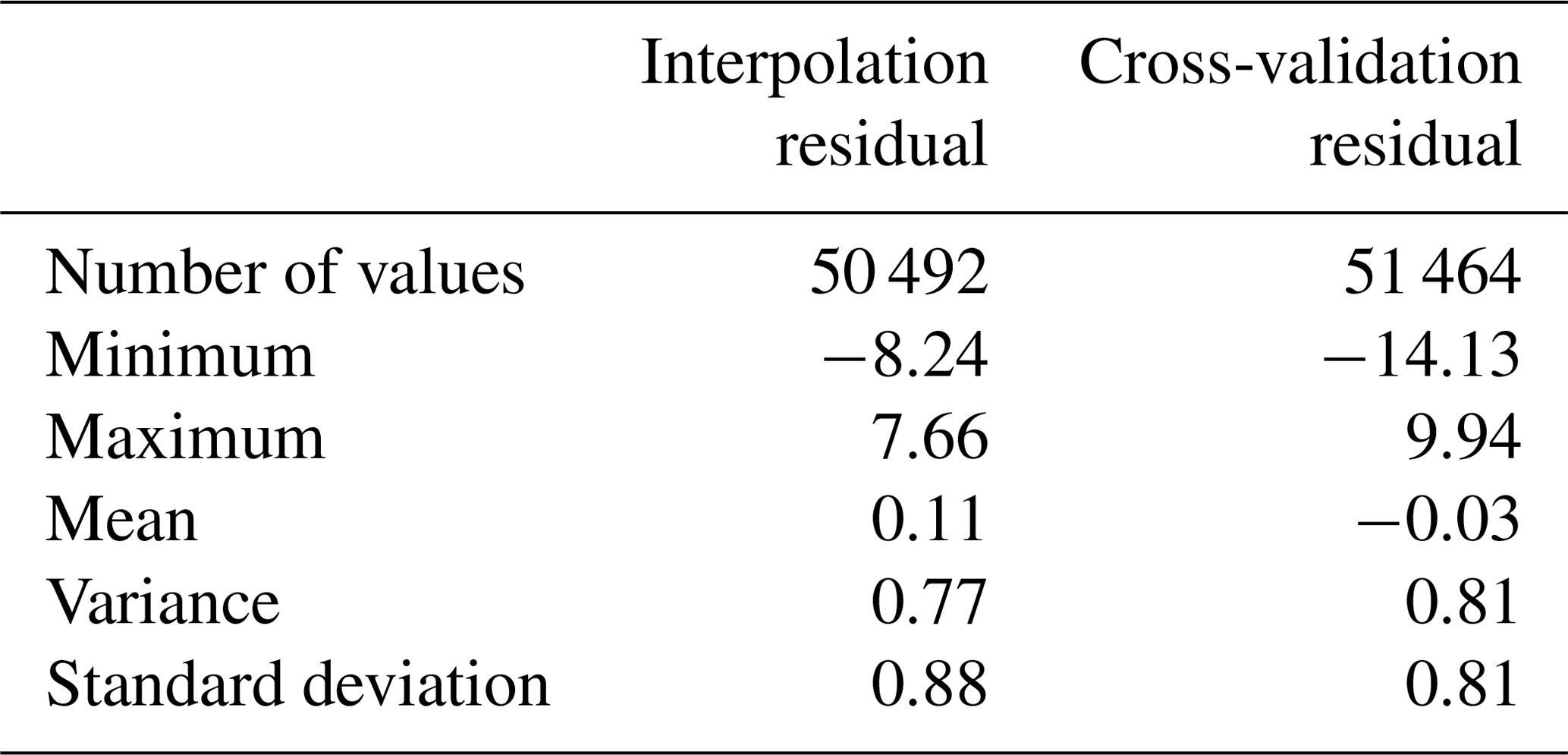
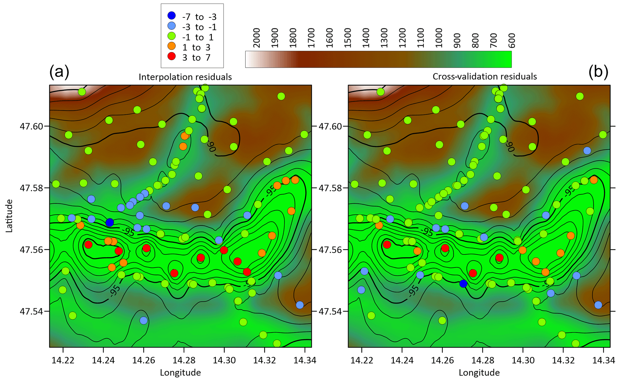
Figure 15Interpolation and cross-validation residuals of a subset within a small section of the Enns valley in Austria. Background image is the topography: contour lines: CBA anomaly (mGal) interpolated using a high-resolution grid (about 200 m spacing); colored dots: residuals (a: interpolation; b: cross validation) at the scattered data points with respect to the AlpArray CBA grid (2000 m spacing). Residuals in milligals (mGal); height in meters.
For discussing the sampling problem, Fig. 15 shows the interpolation residuals (Fig. 15a) and the cross-validation residuals (Fig. 15b) within a smaller section of the Enns valley in Austria. Background colors display the topography, and contour lines show the Bouguer anomaly interpolated to a high-resolution grid with a spacing of 0.00173∘ in latitude and 0.00265∘ in longitude corresponding to a grid spacing of about 200 m. The local negative BA reflects the gravitational effect of the low-density sediment filling of the Enns valley. Colored dots show the residuals as a class scatter plot with respect to the AlpArray grid with about 2000 m spacing. The interpolation residuals range to about 6 mGal along the valley axis, while they are reduced to less than 1 mGal if calculated with respect to the high-resolution grid. Large cross-validation residuals are observed at these stations as well. Given the spacing of 2000 m of the AlpArray grid, the interpolation algorithm does not capture the local anomaly. In this case, the interpolation residuals do not indicate BA errors but reflect the smoothing effect of the coarse AlpArray grid interpolation as was already mentioned in the introduction to Sect. 5.
5.5 Cross-validation error for the entire database
As mentioned in the previous subsection both interpolation residuals and cross-validation methods provide some picture of data quality. At the same time, these methods can be used as a criterion for excluding gross errors from individual databases. Both methods give qualitatively similar results (see Fig. 15), with cross validation giving quantitatively more significant residuals. Since in the case of cross-validation residuals (unlike interpolation residuals) it is possible to exchange data between grid providers in order to comply with the conditions of confidentiality of the original data, we show in Fig. 16 a complete map of cross-validation residuals for the whole area. While the standard deviation of these residuals is well below 1 mGal (comparable to Table 2), the extreme values reach tens of milligals (about 120 points exceed 10 mGal, 9 points exceed 20 mGal). An extreme point with a residual higher than 60 mGal creates a characteristic bull-eye anomaly in the CBA map (Fig. 17). We consider similar points with extreme residuals to be erroneous, and it is therefore necessary to exclude them from the database before compiling the final CBA map. Therefore, it is necessary to choose a reasonable criterion considering the analysis of errors, as well as the problem of inhomogeneous coverage of the territory by the data described in the previous subsections. We decided to use the exclusion criterion of points exceeding interpolation residuals of ±10 mGal. A total of approx. 350 points were excluded (Fig. 18). Except for a few points, almost all excluded points cover marine data, which confirms the naturally lower quality of marine data.
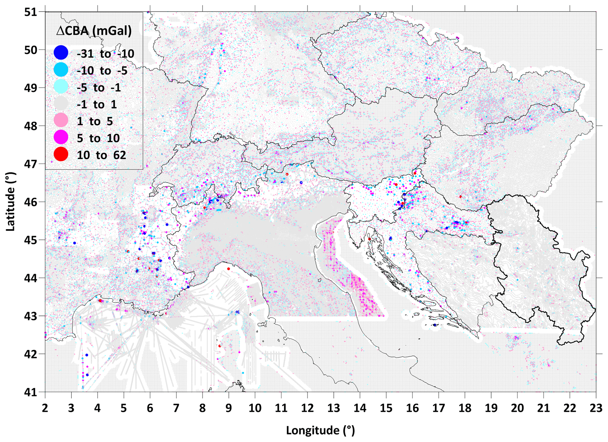
Figure 16Results of cross validation of the new CBA. The point sizes are proportional to the magnitude of residuals. The grey “background” represents locations with lowest residuals.
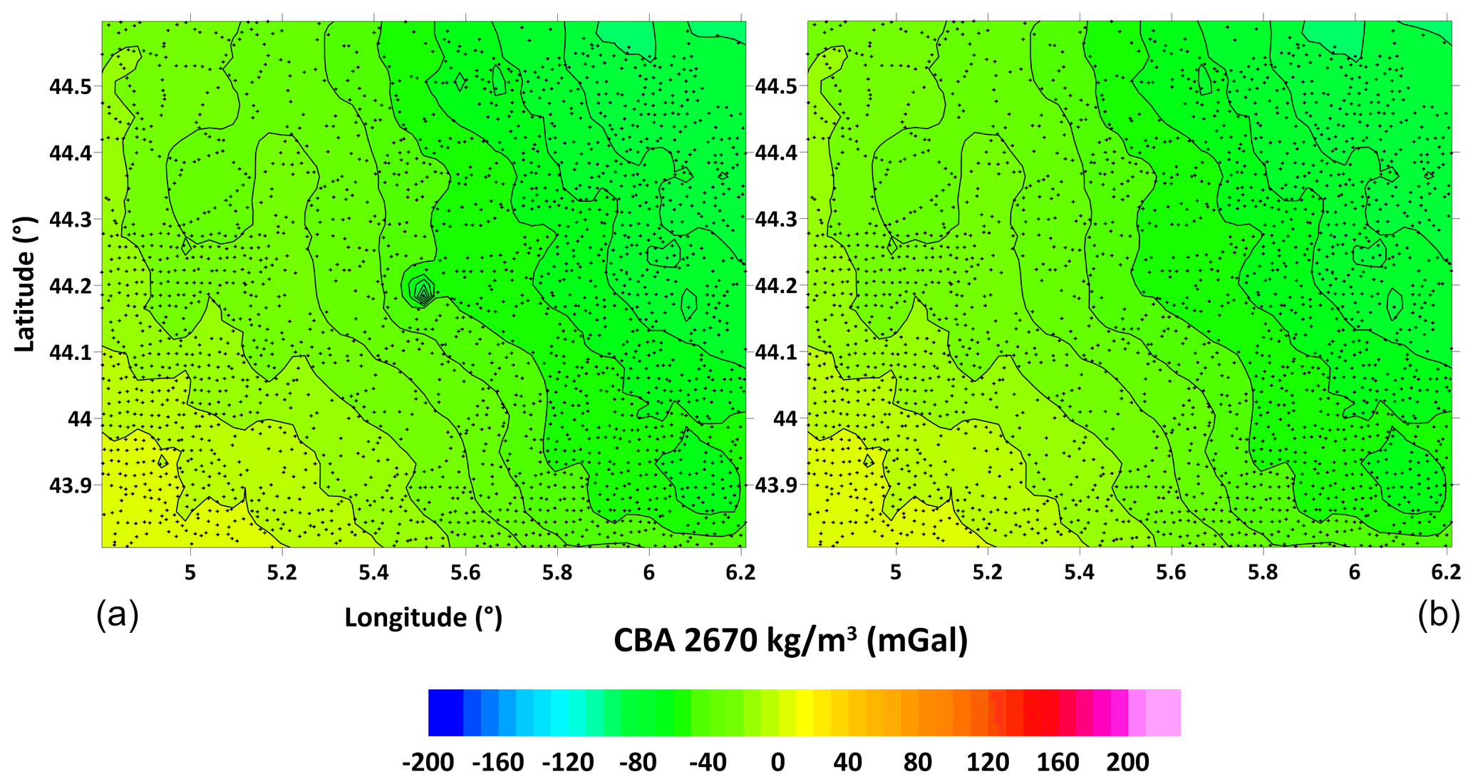
Figure 17Example of an extreme value of more than 60 mGal deviation in the new CBA map: initial CBA version (a) and final CBA version (b). Small black markers represent data points.
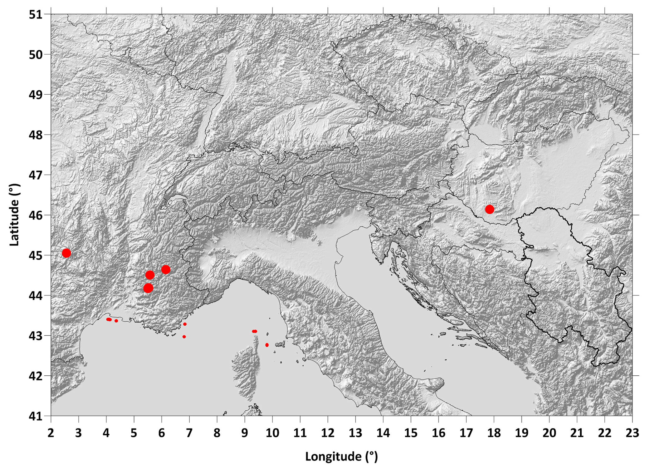
Figure 18Position of excluded points (approx. 350 points in total) based on interpolation residuals higher than ±10 mGal. Almost all excluded points belong to marine data, and very few points lie on land (enlarged points for clarity). The shaded relief in the background shows topography to distinguish land and offshore areas from each other.
From the outset, the AlpArray (AA) initiative was organized in several research groups that contributed to the solution of specific issues. Their main task was to organize and, where appropriate, coordinate the activities of all members within the group. Of the six AA research groups, five were concerned with the solving of seismic problems, and the sixth group had set itself the task of uniformly processing and publishing modern, homogeneous gravity anomalies of land-based gravity data. The results of this group are here presented to the public in two grid versions. In the following, we provide readers (1) with information on the coverage, the acquisition of the data sets and the quality of processed data and (2) their citation, long-term archiving in a data repository and DOI allocation for research data.
6.1 Products
At an early stage, the AAGRG considered which gravity field anomalies in an interdisciplinary work environment could contribute to solving the principal questions posed in the AlpArray program. We hereby make the following anomaly data sets available to the community:
-
The first is free-air anomalies, reconstructed from interpolated Bouguer anomalies according to Eq. (13).
-
The second is complete Bouguer anomalies.
-
In addition, the values of the mass/bathymetric correction will be released in a similar format to the anomalies. Their knowledge is essential because the specification of the values for the mass correction allows for an individual recompilation by the user with a different correction density. This is particularly recommended if the use of an individual density is preferable to the standard density of 2670 kg m−3 in the area under investigation.
-
Also included is the grid of ellipsoidal heights.
The new gridded data sets for the Alpine gravity anomalies are published
-
for the public on a grid of approx. 4 km × approx. 4 km and
-
for the working groups of the AlpArray initiative on a grid approx. 2 km × approx. 2 km.
6.1.1 Coverage and description of data tables
The area covered includes not only the core Alpine regions of the Western and Eastern Alps and the Carpathians but also parts of the Northern Apennines, the Dinarides, the Pannonian Basin and extended Alpine forelands and parts of the Adriatic Sea and the Ligurian Sea. The lower left map corner is located at coordinates 41∘ N, 2∘ E and the upper right at coordinates 51∘ N, 23∘ E.
6.1.2 Relevant specifications
Pan-Alpine_Gravity_ database_2020.dat
This file contains all results organized into seven columns – Lon, Lat, EH, CBA, FA, MC, BC – which respectively correspond to Lon = longitude (decimal degrees, ETRS89), Lat = latitude (decimal degrees), EH = ellipsoidal height (m), CBA = complete Bouguer anomaly (mGal), FA = free-air anomaly (mGal), MC = mass correction (mGal), BC = bathymetric correction (mGal).
The format of the digital grids is as follows.
The five digital grid files
-
“Pan-Alpine_2020_Bouguer_gravity_anomaly_grid.grd”,
-
“Pan-Alpine_2020_free-air_gravity_anomaly_grid.grd”,
-
“Pan-Alpine_2020_mass_correction_grid.grd”
-
“Pan-Alpine_2020_bathymetric_ correction_ grid.grd” and
-
“Pan-Alpine_2020_ellipsoidal_ height_ grid.grd”
are preceded by a header, followed by the array of values as described
below:
| Nx Ny | number of longitude/latitude nodes |
| Xmin Xmax | minimum and maximum values in longitude |
| Ymin Ymax | minimum and maximum values in latitude |
| Zmin Zmax | minimum and maximum values of anomaly |
| Z1 Z2 Z3 Z4 | array of anomaly values; bottom left as the origin (0,0) of the coordinate system. |
Table 3 provides map-relevant information.
Table 3Summary of map-relevant information.
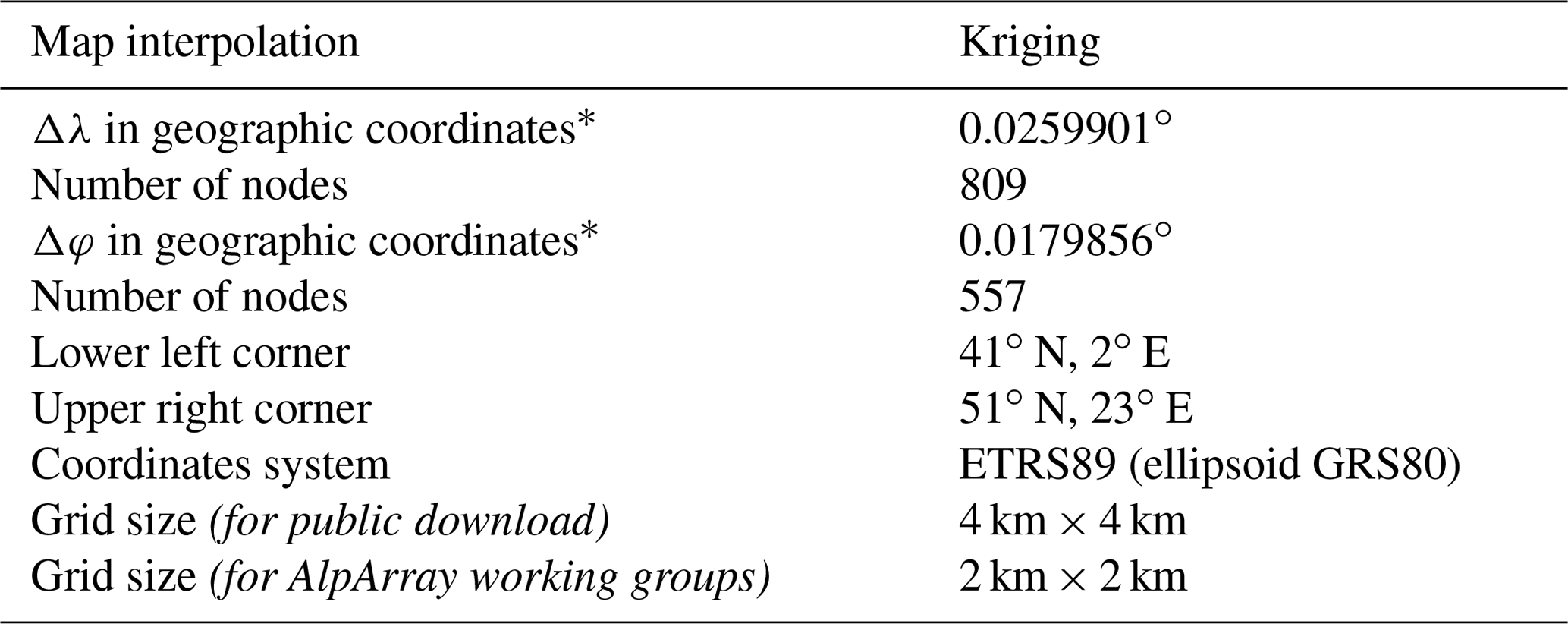
* Note: the agreed area boundaries do not fit exactly with the proposed grid step; so, it was decided to fix the area boundaries and numbers of nodes in longitude and latitude direction. This resulted in somewhat skewed spacing values.
6.1.3 Bouguer gravity map
Although it was and is the declared objective of the AAGRG to compile digital gravity data for the Alps and their adjacent areas, a high-resolution Bouguer gravity map is also available for download in PDF format (Supplement). Besides the anomaly in the form of a “heat map”, it also contains geographic information for better orientation. Figure 19 shows the spatial distribution of all original data considered for the map compilation and all areas where GGM data have been used for filling gaps (refer to Sect. 4.2).
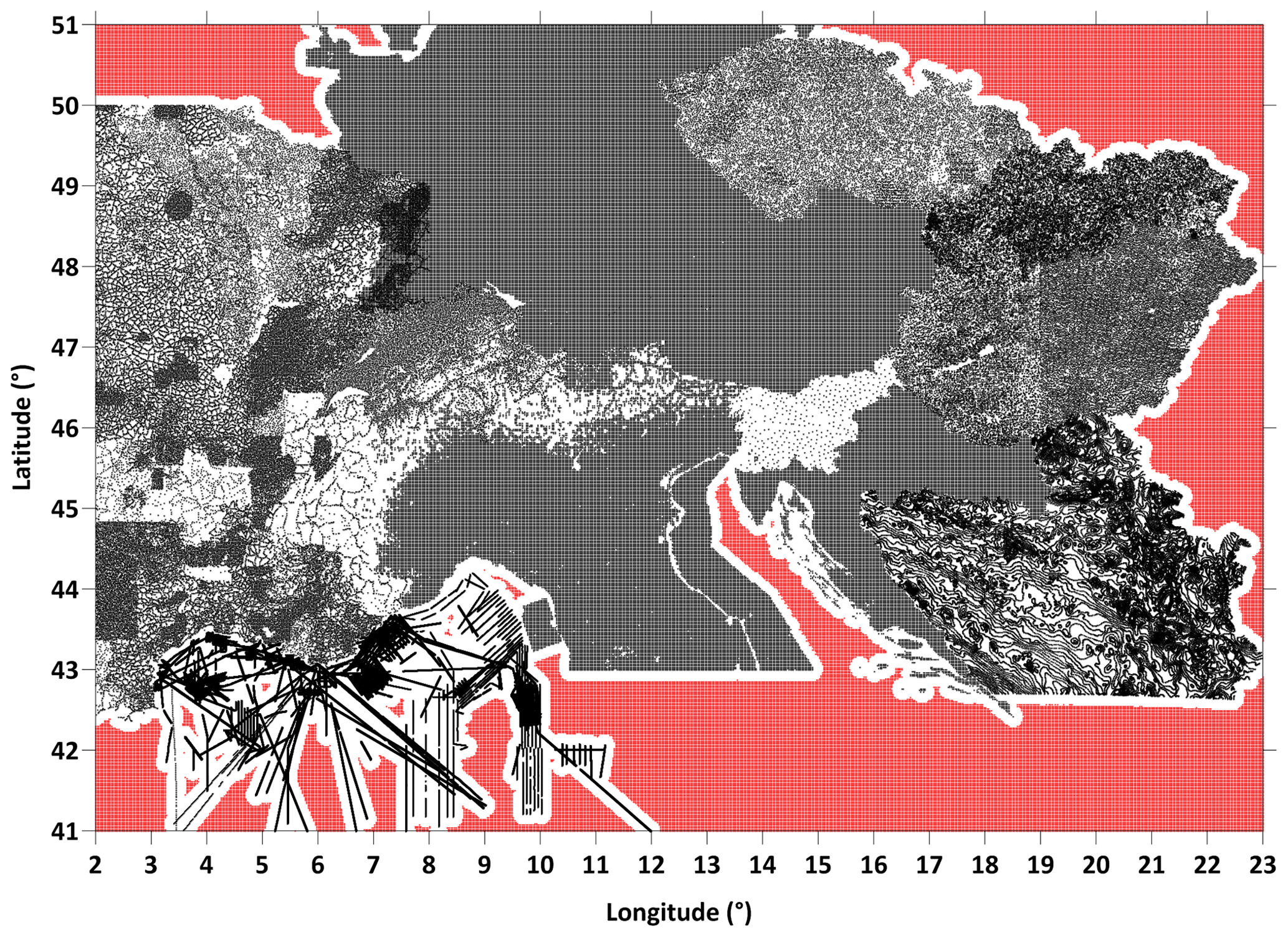
Figure 19Despite all efforts to achieve the greatest possible homogeneity in the database and processing steps, this map is intended to show that the initial database was different due to national requirements. First, the outer areas shown in red are supplements/fillings with GGM values (Sect. 4.2). Irregular black dots indicate the use of point data, and in the offshore areas of the Ligurian Sea black lines indicate the ship tracks. In the southeast of the chart, isolines have been digitized (see also Sect. 3.3).
6.2 Long-term archiving and downloads
The publication and storage of the pan-Alpine gravity data and the accompanying Bouguer gravity map follows the standards of the Alliance of European Science Organisations, which has already declared its support for the long-term storage of open-access data in consideration of disciplinary regulations in the handling of research data in the “Principles for Handling Research Data” adopted in 2010 (DFG in Germany, SNSF in Switzerland, etc.). After the completion of the AAGRG task the group is obliged for various reasons (e.g., AAGRG “Memorandum of Collaboration” with the participating countries, long-term value of the data) to store the data permanently.
GFZ Data Services (http://pmd.gfz-potsdam.de/portal/about.htm, last access: 12 May 2021) is the cooperation partner for data publication via the special information service (FID GEO; https://www.gfz-potsdam.de/zentrum/bibliothek-und-informationsdienste/projekte/fid-geo/, last access: 12 May 2021). The German Research Centre for Geosciences, GFZ, the operator of GFZ Data Services, has been issuing digital object identifiers (DOI) to data sets since 2004 in accordance with the principles of the International DOI Foundation (https://www.doi.org/, last access: 12 May 2021). These data sets are archived and published by GFZ Data Services and cover the entire range of geoscientific activities.
For the gravity data to be found worldwide on the Internet, the data must be given a description that is readable by search engines. This description is provided by metadata. The specific description of metadata for our data set is important but is not part of this publication, but refer to general information in Appendix A.
6.2.1 Data ownership
Data access and use is defined by the AAGRG. The copyrights and access rights are described in a license which is firmly attached to the data and which defines in which way the data may be used or not.
6.2.2 Licenses
The article and corresponding preprints are distributed under a Creative Commons Attribution 4.0 license. Unless otherwise stated, associated material is distributed under the same license.
For the new data sets also a DOI was assigned. They have been published with the DOI https://doi.org/10.5880/fidgeo.2020.045 (Zahorec et al., 2021) and are stored permanently and available in the data repository of the German Research Centre for Geosciences, GFZ. The GFZ has been publishing geoscientific research data since 2004 and guarantees technical integrity and long-term availability.
The aim of this publication is to report on the activities and work of the AlpArray Gravity Research Group (AAGRG) over more than 3 years. The group's mission was to recompile and release digital homogenized gravity data sets that are based on terrestrial gravity measurements that are owned by the national Alpine neighboring countries (in total more than 1 million data points). They can be used for high-resolution modeling, interdisciplinary studies from continental to regional and even to local scales, and for joint inversion with other data sets. Bouguer and free-air anomalies are available at a grid density of 4 km × 4 km for the public and of 2 km × 2 km for internal AlpArray use on request. The final products also include grids for mass and bathymetric corrections of the measured gravity at each grid point. This allows for the use of later customized densities for their individual calculations of mass corrections between the physical surface and the ellipsoidal reference.
Both digital data sets are compiled according to the most modern geophysical and geodetic criteria and reference frames (both location and gravity). This includes the concept of ellipsoidal heights and implicitly includes the calculation of the geophysical indirect effect; atmospheric corrections are also considered. For the calculation of station-completed Bouguer anomalies, we used the following densities: 2670 kg m−3 for landmasses, 1030 kg m−3 for water masses above the ellipsoid and −1640 kg m−3 for those below the ellipsoid. The mass correction radius was set to Hayford zone O2 (167 km). Special emphasis was put on the numerous lakes in the study area. They partly have a considerable effect on the gravity of stations that lie at their edges (for example, the rather deep reservoirs in the Alps). In the Ligurian Sea, ship data of the Service Hydrographique et Océanographique de la Marine and of the Bureau Gravimétrique International were implemented in the digital database. Although not unproblematic, these data got the preference over satellite data offshore.
In the future, the calculation of long-distance effects of topography and bathymetry and their compensating masses (roots) are planned. What is absolutely necessary is a more profound analysis of the map uncertainties. The associated research is complicated by the fact that for many of the national data sets used, no metadata are available. The reasons for this are manifold and do not lie with the group. To obtain an estimate of the error size in the present compilation, cross validations were calculated both for the entire grid and for the national grids. After an iterative improvement by the elimination of erroneous data, a map error of max. ±5 mGal can be assumed after the third iteration. In some offshore areas the error is less than 10 mGal.
| AAGRG | AlpArray Gravity Research Group |
| BC | Bathymetric correction |
| BEV | Federal Office of Metrology and Surveying, Vienna, Austria |
| BGF | Banque Gravimétrique de la France |
| BGI | Bureau Gravimetrique International |
| BRGM | Bureau de Recherches Géologiques et Minières |
| CAGL | Central Apennine gravity low |
| CBA | Complete Bouguer anomaly |
| CGF65 | Carte Gravimétrique de la France 1965 |
| CGG | Compagnie Générale de Géophysique |
| CNEXO | Centre National pour l'Exploitation des Océans |
| CV | Cross validation |
| DEM | Digital elevation model |
| DEM25 | Digital elevation model (25 m resolution, Germany) |
| DGL | Dinaric gravity low |
| DHHN | German main leveling network |
| DTM | Digital terrain model |
| DRE | Distant relief effect |
| EGM2008 | Earth Gravitational Model of 2008 |
| EIGEN (6C4) | European Improved Gravity model of the Earth by New techniques (6C4) |
| EMODnet | European Marine Observation and Data Network |
| ETRS89 | European Terrestrial Reference System 1989 |
| EOV | Hungarian geodetic coordinates in national map projection |
| EVRS | European Vertical Reference System |
| FA | Free-air anomaly |
| GEBCO | General Bathymetric Chart of the Oceans |
| GGM | Global gravitational model |
| GIE | Geophysical indirect effect |
| GIS | Geographic information system |
| GNSS | Global navigation satellite system |
| GPS | Global positioning system |
| GRAVI-CH | Gravity database of Switzerland |
| GRS80 | Geodetic Reference System from 1980 |
| HVRS1971 | Croatian Height Reference System from 1971 |
| IAG | International Association of Geodesy |
| IFREMER | Institut Français de Recherche pour l'Exploitation de la Mer |
| IGF | International gravity formula |
| IGFS | International Gravity Field Service |
| IGH | Ivrea gravity high |
| IGN | Institut de l'Information Géographique et Forestière |
| IGSN71 | International Gravity Standardization Net 1971 |
| IUGG67 | International Union of Geophysics and Geodesy, 1967 congress |
| LCC | Lambert conformal conic (projection) |
| Lidar | Light detection and ranging |
| LN02 | Height system of Switzerland |
| MC | Mass correction |
| MERIT DEM | Multi-error-removed improved-terrain DEM |
| MGH | Hungarian gravity network |
| MGHi | Mediterranean gravity high |
| NAGL | Northern Apennine gravity low |
| NTE | Near-terrain effect |
| OGS | National Institute of Oceanography and Experimental Geophysics |
| OMV | AG Österreichische Mineralölverwaltung AG |
| PBGH | Pannonian Basin gravity high |
| RCGF09 | Gravimetric Network and Map of France 2009 |
| RGF83 | Réseau Gravimétrique Français |
| RMS | Root mean square |
| RTM | Residual terrain modeling |
| SAPOS | Satellite Positioning Service of the German Surveying and Mapping Agency) |
| SDB | Satellite-derived bathymetry |
| SGr-57, 67, 95 | Czech and Slovak National Gravimetric System of 1957, 1967 and 1995 |
| SKPOS | Slovak real-time positioning service |
| SHOM | Service Hydrographique et Océanographique de la Marine |
| SI | Système international d'unités (international unit system) |
| SRTM | Shuttle Radar Topography Mission |
| TC | Terrain correction |
| TM | Transverse Mercator (projection) |
| UTM | Universal Transverse Mercator (projection) |
| VFGL | Venetian/Friuli Plain gravity low |
| WCGL | Western Carpathian gravity low |
| WGS84 | World Geodetic System 1984 |
Appendix B provides the historical activities of the main actors at first and then the national contributions to the pan-Alpine Bouguer gravity map.
B1 Historical activities
B1.1 Austria
Zych (1988) reports on the first gravity measurements in Austria in the course of hydrocarbon exploration as early as 1919, while more intensive, regional and detailed measurements were carried out in the following years with pendulums, torsion balances and gravimeters, concentrating mainly on the Vienna Basin and neighboring areas. This and other measurements were later included in the gravity map of Austria (Senftl, 1965) by the Federal Office of Metrology and Surveying (BEV) at a scale of 1:1 million. BEV, several universities in Austria (Vienna, Leoben) and Germany (Clausthal-Zellerfeld), and the hydrocarbon industry (OMV AG, Austria) added numerous gravity profiles and areal networks across the Austrian territory since then (see, e.g., Meurers, 1992a, b; Steinhauser et al., 1990; Götze et al., 1979). In 2009, Meurers and Ruess published a complete review of the gravity values measured in Austria, “A new Bouguer Gravity Map of Austria” (Meurers and Ruess, 2009), on the basis of 54 000 land gravimetric data points. These recompilations already contained most of the numerical approaches that have been implemented in our new pan-Alpine Gravity Map.
B1.2 Switzerland
An early compilation of gravity measurements and a gravity map covering the entire country was published in 1921 based on data acquired since 1900 (Niethammer, 1921). In 2008, the Institute of Geophysics of the University of Lausanne published the gravity map of Bouguer anomalies in Switzerland at a scale of 1:500 000 for the Swiss Geophysical Commission: editors were Olivier et al. (2010), and their compilation was based on the work of Klingelé and Olivier (1980). It reflects the culmination of more than 15 years of work and effort on the part of many staff and students at the Geophysical Institutes of the University of Lausanne and the Polytechnic School of Zurich. Between 1994 and 2002, a set of 22 1:100 000 scale maps of Bouguer anomalies was published. The anomalies were calculated with the 1967 ellipsoid with a density of 2670 kg m−3 and which corrected for relief up to a distance of 167 km around each station. These maps were elaborated from 29 900 measured stations selected from the gravity database GRAVI-CH over a territory of about 56 000 km2. In total, approx. 85 gravimetric campaigns were carried out between 1986 and 2000. The Swiss experience with the Bouguer gravity compilation was also exemplary for the creation of a common gravity database in the entire Alpine region.
B1.3 France
A detailed and systematic gravimetric coverage of the French territory was conducted in the frame of the Carte Gravimétrique de la France 1965 (CGF65). The establishment of a reference network of 2000 base stations originally linked to international absolute stations (Potsdam system) and the gravity surveys carried out between 1945 and 1975 using North American, LaCoste and Romberg, and Worden meters for mapping, mineral and oil prospecting, or for academic purposes provided the first gravity infrastructure at national scale. Despite incomplete coverage, it was published in 1975 in the form of a map on a scale of 1:1 000 000 (north and south sheets). The primary reference network was later updated as the Réseau Gravimétrique Français (RGF83) with additional absolute gravity measurements and links to the IGSN71 international network. The digital recording of available terrestrial gravity data acquired by several organizations (Bureau de Recherches Géologiques et Minières, BRGM; Institut de l'Information Géographique et Forestière, IGN; oil and mining companies; universities and research institutes) was started in 1977. In 1990, BRGM founded the “Banque Gravimétrique de la France” (BGF) to manage and update the stations on the French gravity map. The BRGM database is also periodically submitted to the “International Gravimetric Bureau” (BGI) for data distribution and contribution to the global gravity mapping.
B1.4 Italy
One may speculate that the history of gravity measurements worldwide and especially in Italy began with the free fall experiments of Galileo Galilei (1564–1642). In his honorary capacity we still use gals or milligals (10−5 m s−2) even today. The 1980s and 1990s of the 20th century were characterized by the development of an absolute gravity meter (Istituto di Metrologia G. Colonnetti) for on- and offshore measurements (Gulf of Naples and 2000 km gravity profiles in the Mediterranean Sea) in connection with European geodesy projects.
In 1975 the late Italian Geodetic Commission decided on the compilation of a new Bouguer anomaly map of Italy based on up-to-date correction standards and homogeneous methodology. This map was published in 1991 by the National Research Council (CNR; C.N.R.-P.F.G., 1992) as part of the Structural Model of Italy at a scale of 1:500 000. The gravity values were referred to IGSN71 (Morelli et al., 1972), density for the terrain correction was set to 2400 kg m−3, and the main data contribution was from the Italian National Oil Company (ENI-AGIP).
In 1989 the Geological Survey of Italy, together with ENI-AGIP, published a new gravity map of Italy scaled at 1:1 000 000 using the data set collected for the 1:500 000 CNR gravity map. In the 1990s the Geological Survey of Italy undertook an extensive land gravity cartography program that has covered the whole national territory at the scale of 1:50 000. The presently available gravity map from the Department of Terrain defense – National Geological Survey of the “Italian Agency for Environmental Protection and Technical Services” (APAT) is a map published at the scale of 1:1 250 000 published in 2005 (APAT, 2005; Ferri et al., 2005), which used a terrain correction density of 2670 kg m−3 and the Hayford radius of 166.736 km. Data were collected from different sources, such as ENI, OGS, the US Defense Mapping Agency, academic organizations and the former Italian Geological Survey. Station density in the Alps for this map is about 0.1 to 0.2 stations per 1 km2, and it increases to 1.5 stations per 1 km2 in the basins. The Bouguer anomaly has been corrected for topography onshore, whereas for offshore a free-air anomaly map was published.
B1.5 Slovenia
The first map of Bouguer anomalies which comprises the whole Slovenian territory was compiled in 1967 (Čibej, 1967; Ravnik et al., 1995). It was based on data measurements with a Worden gravity meter (no. 117) in the framework of various gravity surveys conducted over the period 1952–1965 by the Geological Survey of Slovenia (Stopar, 2016). Later in the frame of the W–E Europe Gravity Project led by Getech from Leeds University, a new data set was prepared in the 1990s which comprises 416 gravity points giving an average density of 0.02 gravity stations per 1 km2. Gravity data in Slovenia reflect a complex structural setting in the transition area between the Alps, Carpathians, Dinarides and Pannonian basin. Large variations in the crustal thickness (Gosar, 2016) and the depth of sedimentary basins in the transition from the Alps–Dinarides to the Pannonian basin in Slovenia are clearly reflected in Bouguer anomalies.
B1.6 Germany
With the start of the Deutsche Reichsaufnahme in 1934, an important development phase also began for gravity in Germany. Gravimetric maps were produced by the Amt für Bodenforschung which supplemented mainly the Alpine foreland. After 1945, the Amt für Bodenforschung coordinated the first efforts to complement this database in West Germany. Gerke (1957) published the gravity map of West Germany (cited from Closs, 2008). The Bouguer gravity map at a scale of 1:500 000 of the Federal Republic of Germany was produced by Siegfried Plaumann (e.g., sheet south – now referred to IGSN71; Plaumann, 1995) on the basis of measurements by the Geophysical Survey of the Federal Republic of Germany, the Lower Saxony State Office for Soil Research, and oil companies. After corrections of the gravity meter drift and terrain, they were reduced to sea level with a density of 2670 kg m−3 and referred to IGSN71.
B1.7 Hungary
Gravity field investigations and field observations in Hungary were already established by the pioneering work of Baron Loránd (Roland) Eötvös. The Eötvös torsion balance became the world's first geophysical tool for prospecting, and it revealed hundreds of hydrocarbon resources; see Szabó (2016) for a full narrative of the history.
B1.8 Slovak Republic
A thorough overview of the practical and methodological developments of gravimetry in the Slovak Republic can be found in Understanding the Bouguer Anomaly – A Gravimetry Puzzle (Pašteka et al., 2017). The territory of the Slovak Republic (except the inaccessible areas of the Tatra Mountains) is covered by regional gravity measurements at the scale of 1:25 000 with station spacing from three to six stations per 1 km2. The measurements were realized during a long period from the 1950s up to the 1990s. The project's goal was to create a high-definition gravity map for mineral exploration and basic geologic interpretations. Various types of gravity meters were used during the data acquisition time period (GAK PT, Worden, Canadian CG-2, Scintrex CG-3M). Different approaches to complete Bouguer anomaly (CBA) calculation were used, including different normal field formulas, different equations for “Bouguer” correction and atmospheric correction, and various methods of the terrain correction estimation. A complete recalculation of the entire database was performed in the frame of the earlier project Atlas of geophysical map and lines (Grand et al., 2001). Several hundreds of points with errors in their heights or positions were identified – these points had been removed from the final Bouguer anomaly evaluation.
B1.9 National contributions
After this historical review we describe country by country the initial situation for the assessment and application of existing data, available publications, data density, and quality. The following partner and AAGRG member countries have contributed to the compilation of the new pan-Alpine gravity maps.
Austria
In the early beginning, gravity stations in Austria were mainly arranged along leveling lines. The first areal network, which was surveyed by OMV (Österreichische Mineralölverwaltung), focused on the Alpine Foreland, the Vienna basin and parts of the Flysch and Calcareous zone of the Eastern Alps (Zych, 1988). Additional gravity profiles were established across the central part of the Eastern Alps (Ehrismann et al., 1969, 1973, 1976; Götze et al., 1978) 50 years ago. The vertical coordinates of all stations so far were determined by precise leveling, while horizontal coordinates were based on topographic map digitization providing an accuracy estimate of ±25 m. The first area design with stations even on high mountain flanks and peaks started during the late 1970s (Götze et al., 1979; Schmidt, 1985; Meurers et al., 1987; Posch and Walach, 1990; Walach, 1990; Winter, 1993). Most of the new stations were established at benchmarks of the national cadastre with maximum coordinate errors of a few tens of centimeters in height and even better accuracy in horizontal positions, even on high mountains. However, in large areas, particularly along the Alpine crest, station coverage was sparse. Since 1982, GPS techniques and helicopter transportation in otherwise inaccessible mountainous regions also made these areas accessible while meeting modern accuracy requirements. Presently the Austrian gravity database contains about 54 000 stations with an average station interval of less than 3 km even in the high mountains and average station density of one station per 9 km2 or more. In the early gravity campaigns Askania and Worden gravimeters were used, and since 1970 only LaCoste and Romberg or Scintrex gravimeters have been used. Depending on the data provider and acquisition date, data referred to different reference systems and exhibited different accuracy. In addition, industrial data (OMV) were tied to a gravity base which had a slightly different scale due to limited calibration accuracy. For the most recent gravity map of Austria (Meurers and Ruess, 2009), all data were homogenized regarding height and gravity data based on ties to the Austrian absolute gravity network (Ruess, 2002; Meurers and Ruess, 2007). Gross coordinate errors were detected by comparing station heights with interpolations of a high-resolution digital terrain model with 50 m spacing. Erroneous coordinates were corrected by using modern topographic and orthophoto maps and by utilizing the digital cadastre (Meurers and Ruess, 2007). Based on modern methods of terrain correction procedures, digital terrain models and a new geoid model (Pail et al., 2008), the Bouguer anomaly of Austria was determined using for the first time ellipsoidal heights (Meurers and Ruess, 2009). The exact transformation from local Gauß–Krüger coordinates and orthometric heights into ETRS89 UTM and WGS84 geographical coordinates was done by applying a stepwise procedure recommended by the national surveying office (BEV, http://www.bev.gv.at, last access: 12 May 2021).
Croatia
The Croatian national gravity database consists of approximately 16 500 free-air anomaly values covering the entire continental area. Data in the database were mainly collected from 1945 to 1990 across the territory of the former Socialist Federal Republic (SFR) of Yugoslavia. The data are almost equally distributed across the wider territory of Croatia, also including some points in Bosnia and Herzegovina and Slovenia. The average point density is 1 point per 18 km2; in the continental part of Croatia data density is 1 point per 8 km2, whereas in mountainous areas and on islands density is much lower (one station per 30 km2). Each point has appended geodetic coordinates referring to GRS80 ellipsoid, whereas heights are normal-orthometric referring to the national height reference system, Croatian Height Reference System (HVRS1971). Gravity values refer to the International Gravity System Network of 1971 (IGSN71). Metadata about the accuracy of gravity values, position and heights do not exist. Since its creation the database passed through several phases of checking, cleaning, debiasing and filtering. It was used in geophysics for creating Bouguer anomaly maps (Bilibajkič et al., 1979) in the past. Most recently, it found specific usage in national geoid model determination (Bašić, 2009; Varga, 2018). For the purposes of the AAGRG project all available points were included in the gridding of the model of Bouguer anomalies.
Czech Republic and Slovak Republic
Equally for the Czech Republic and the Slovak Republic, most regional gravity surveys were conducted from the 1950s till the 1990s. The prevalent sampling interval was about 500 m, or five stations per 1 km2, during the so-called “mapping 1:25 000” scale. This mapping covered about 75 % of the Czech Republic and 100 % of the Slovakian territory, while the rest was previously covered by mapping at a 1:200 000 scale with about one station per 4 km2. Principal targets of the surveys were mineral exploration for uranium, tin and other minerals, oil and gas, and hydrological and environmental investigations, as well as basic geological research. The database was reduced to a 2 km×2 km coverage and now contains 13 955 points for the Czech Republic and 21 108 points from the Slovak Republic. Positions of the stations were digitized from the “military topographic maps” at the scale of 1:25 000 in a Gauß–Krüger projection coordinate system. The accuracy in the positions of these points is in the range of 10–50 m. Heights of the gravity points were determined in the Baltic vertical reference system by geodetic leveling connected to the points of the national leveling network. Vertical accuracy ranges from 5 cm in the lowlands to 50 cm in the mountains. Gravity values were tied to the “National Gravimetric System SGr-57, 67” which is connected to the old Potsdam system. Consequently, they were transformed to the recent absolute gravimetric system SGr-95. Accuracy of the gravity values is up to 100 µGal.
Further parameters of this exemplary new compilation are the use of the Somigliana–Pizzetti formula for normal gravity, the spherical calculation of the topography effect (density 2670 kg m−3), free-air correction term and atmospheric correction. In addition to the mentioned standard steps of the CBA calculation, effects of the distant topography, bathymetry and ice sheet effects were calculated for the entire database. The expertise gained was fully available for the compilation of the Alpine gravity map.
One of the most important steps of this process is the precise evaluation of the terrain corrections. For selected areas of Slovakia gravity maps were compiled and purpose-derived gravity maps, and density models were constructed along selected regional gravimetric profiles across the territory of the Western Carpathians. The first map in the Czech Republic was made accessible to the public in April 2009, was last updated in April 2013 and was turned into a world-wide-web format in 2014.
France
Since the early 1990s, gravity densifications have been realized using Scintrex gravity meters (CG3, CG5 and currently CG6) and accurate GPS positioning, mainly as part of major scientific projects such as GéoFrance3D (“Millennium Project”). A new gravity database based on both recalculated corrections with a density of 2670 kg m−3 and on the IGSN71 system using data from the BGF and other sources (Grandjean et al., 1998) was established. A new gravity map of France, including terrain corrections uniformly computed up to 166.7 km, was released by BRGM (Martelet et al., 2009) in the frame of the RCGF09 action (Gravimetric Network and Map of France 2009), which also led to the joint creation of a new gravimetric network by IGN. Since 2006, hybrid relative (Scintrex) and absolute (Micro-g A10) gravity surveys have been carried out by IGN for defining a first-order precise gravity reference network (RMS 25 µGal) of over 1200 stations. Nowadays, the complete gravity coverage of the French territory contains approximately 370 000 points. All this gravity information is currently used to refine the computation of the national geoid, of the gravity anomalies and of the height conversion grids.
The gravity data sets over France and the surrounding marine areas are provided from the BGI global gravity databases (http://bgi.obs-mip.fr/, last access: 12 May 2021). Terrestrial data are mostly derived from the gravity surveys carried out and compiled by BRGM. They also include 2272 gravity data points in the Alps provided by IGN and other contributions from by Guglielmetti et al. (2013) and research laboratories (Paris, Toulouse, Montpellier, Strasbourg, Clermont-Ferrand, Grenoble and Nice). Finally, the data set has been sampled with 1 point per 4 km2 giving a total amount of 22 593 free-air gravity values over the French territory concerned.
Offshore data
Offshore gravity measurements in the study area were collected from shipborne surveys performed since the 1960s in the Gulf of Lyon and Ligurian Sea by the French IFREMER, CNEXO, SHOM and CGG. In addition, this area is also covered by the extensive gravity surveys carried out between 1961 and 1972 by the Italian Experimental Geophysical Observatory over the whole Mediterranean Sea, and it is known as the “Morelli dataset” (Allan and Morelli, 1971). These surveys were conducted with different generations of sea gravity meters (LaCoste and Romberg, Graf-Askania, Lake Constance) mounted on a gyro-stabilized platform. Corresponding gravity data and reports are archived by IFREMER and SHOM and transmitted to the BGI.
Offshore gravity data included in the AlpArray compilation are provided by the GEOMED2 project (Lequentrec-Lalancette et al., 2016; Barzaghi et al., 2018). This project was recently conducted in the frame of the International Association of Geodesy (IAG) by the International Gravity Field Service (IGFS) and BGI, and it aimed at providing high-resolution geoid and gravity grids and maps of the whole Mediterranean Sea. The compilation, validation and adjustment of the above-mentioned French and Italian marine gravity surveys were done by SHOM and BGI considering the usual protocols applied at SHOM (Service Hydrographique et Océanographique de la Marine) for the qualification of marine gravity data. The final GEOMED2 product led to the realization of a 1 arcmin×1 arcmin free-air gravity grid for the whole Mediterranean Sea given in the IGSN71 reference system with an estimated accuracy of 3.6 mGal deduced from the internal and external crossover analysis. Details of the gravity data acquisition and compilation can be found in Lequentrec-Lalancette et al. (2016).
Germany
The German data used in the AlpArray project originate from three main data sets that were acquired between ca. 1930 and 2010. The AlpArray area is covered by 36 442 gravity stations. As only a few historical measurements were carried out in the frame of dense local surveys, the mean point spacing is on the order of 2 to 3 km. Regional gravity measurements were either conducted at public geodetic reference points, for which precise coordinates were available, or at prominent points that could be easily identified in maps and for which coordinates were digitized. Hence, the precision of the coordinates can vary between some centimeters and some tens of meters. The heights of the German gravity stations refer to the reference system DHHN (German main leveling network) and the version valid at the time of the measurement. This may result in deviations from the current reference system DHHN2016 on the order of some centimeters. During the reprocessing in 2010, station heights were checked for plausibility by a comparison with heights taken from the DEM25 (the best German DEM at that time). As large deviations can also result from imprecise horizontal coordinates of the stations, such stations were additionally evaluated with respect to their location by means of GIS techniques and, if necessary, by an additional comparison with georeferenced digital topographic maps and orthophotos. For 95 % of the stations covering the entire German territory the differences in height are less than 2 m. Gravity stations that exhibit differences of more than 5 m to DEM25 were not considered in the data contribution for the compilation of the new AlpArray Bouguer gravity map.
The current Bouguer anomaly map for Germany (Leibniz-Institut für Angewandte Geophysik, 2010; Skiba, 2011), based on more than 275 000 data points, refers to the IGSN71 and a density of 2670 kg m−3. Absolute gravity values that were acquired in the old Potsdam gravity system were transferred to the IGSN71. The accuracy of the absolute gravity is estimated to be better than 100 µGal.
For the AlpArray compilation, gravity data were provided by the Leibniz Institute for Applied Geophysics (including data from the Geophysikalische Reichsaufnahme), Kiel University and the Geological Survey of Saxony (LfULG).
Hungary
Hungary contributed to the unified Bouguer gravity map with gridded data of 2 km × 2 km given in Gauß–Krüger map projection, and the terrain correction was calculated up to a distance of 22.5 km around each station utilizing a uniform reduction density of 2670 kg m−3.
The Hungarian gravity database consists of approximately 388 000 data points and covers the whole country with rather heterogeneous point density. Gravity measurements were mainly carried out between 1950 and 2010 for different purposes, which determines the point distribution. For the oil industry, local exploration grids were established with a few hundred meters grid spacing; on the other hand, due to transportation requirements, early measurements were arranged along roads. The average point density of 2.8 points per 1 km2 suggests a fair coverage, but it concentrates on areas with low to moderate topography. The database consists of geodetic coordinates given in the national map projection (EOV) system with reference to the IUGG67 ellipsoid, whereas heights are given in the Baltic height system. Gravity values are tied to the Hungarian gravity network MGH (from Hungarian abbreviation), which was established, extended and readjusted in several epochs (MGH-50, MGH-80, MGH-2000, MGH-2010 and MGH-2013 networks; Csapó and Völgyesi, 2002; Csapó and Koppán, 2013; Csapó, 2013) to unify gravity values, support regional-scale data processing and to connect to the Unified European Gravimetric Network. Metadata on the accuracy of horizontal position, height and gravity data are not provided in the data set. The estimated accuracy of g values is 0.1 mGal on average. The database was collected and is maintained by the Mining and Geological Survey of Hungary. Following the requirements for the new pan-Alpine Bouguer model, the high-resolution national digital elevation model with spacing of 30 m × 30 m was used in the computation of the gravitational effect of nearby terrain masses. The DEM was produced by digitizing the isolines of the topographic maps on the scale of 1:10 000.
Italy
The Italian data used in the AlpArray project originate from one main data set, which is industry data handed over by ENI, and several other minor data sets, including the Province of Bolzano, newly acquired data in the Ivrea–Verbano zone preferentially to fill earlier data gaps (Scarponi et al., 2020), data acquired in the Province of Bolzano during the INTAGRAF project, and SwissTopo data. The AlpArray area is covered by 130 905 gravity stations, of which the ENI data set has 128 479 stations on land and offshore, in the Province of Bolzano there are 1737 stations, and in the Ivrea–Verbano area there are 689 stations. The data are very dense in the Po plain and scarcer at the higher elevations, with a mean point spacing of 705 m. Gravity measurements other than ENI were conducted at cadastral geodetic reference points for which precise coordinates were available or were acquired at a position and height with parallel GNSS observations. The ENI data points were acquired with either traditional geodetic survey or the newer points with GNSS. The positions of the Italian gravity stations refer to the reference system GRS80, with the industry data having been transferred to GRS80 in the frame of a revision of the database and with the heights in normal heights. Geoidal heights were converted to ellipsoidal heights by adding the ITALGEO geoid heights. We have compared the normal heights with different terrain models, with MERIT (Yamazaki et al., 2017) and in the Region Veneto with the local high-resolution DEM. The average difference with MERIT of the entire database is 0.3 m, and the root mean square difference is 12.63 m. The criterion for using a data point for the final map was a difference with MERIT of less than 50 m. This large height difference is limited to relatively higher elevations outside the plains and is probably due rather to the sparse grid-spacing of the MERIT model than to misplacement of the stations. We find that 66.64 % and 79.57 % of the entire onshore database has a height error below 5 m and below 10 m compared to MERIT, respectively. The absolute values of the ENI database referred to the old Potsdam gravity system and were transferred to the IGSN71, correcting the values for 14.00 mGal (Morelli, 1948; Wollard, 1979). In the areas with both ENI data and modern acquired data, the systematic shift was confirmed by direct comparison of the absolute gravity values.
Slovenia
From the gravity map of the Geological Survey of Slovenia (Čibej, 1967) approximately 2150 gravity points were selected for the construction of the regional map at the scale of 1:100 000. Gauß–Krüger coordinate system was used and later transformed to WGS84. The average density of gravity points of this data set is 0.106 points per 1 km2. The map was digitized and re-interpolated between 1996 and 2000 by Stopar (2016). All gravity measurements were tied to the national gravity system which was linked to the Potsdam system. The average density of gravity points of this data set is 0.106 points per 1 km2. In the original data set (Čibej, 1967) terrain corrections were computed up to the distance of 20 km. For the purpose of AAGRG compilation, digital elevation models (DEMs) for Slovenia in 12.5 m×12.5 m grid sizes prepared from orthophoto surveys were used for terrain corrections. The general estimated accuracy of the model is 3.2 m: more specifically, in flat areas 1.1 m, low hills 2.3 m, medium hills 3.8 m and mountain areas 7.0 m (Surveying and mapping authority of Slovenia, 2019). Application of a high-resolution 1 m grid size DEM based on a recent lidar survey of the whole of Slovenia was also considered.
In the frame of the W-E Europe Gravity Project led by Getech from Leeds a new data set was prepared in the 1990s which comprises 416 gravity points giving an average density of 0.02 stations per 1 km2 (Car et al., 1996). The Gauß–Krüger coordinate system was used and later transformed to MGI 1901 Bessel and WGS84. The data and reference field was Potsdam 1967 in the IGSN71 system with added atmosphere correction. Terrain corrections were computed up to the distance of 167.7 km using the density of 2670 kg m−3. The estimated accuracy of this data set is 0.05 mGal in flat areas and much lower in mountain areas.
Switzerland
The Swiss gravity database GRAVI-CH was collected and maintained by the University of Lausanne (Olivier et al., 2010). It consists of around 30 000 points with measurements from 1953 to 2000.
The data set used in this project is a subset of 7962 points from GRAVI-CH, limited to the area of Switzerland and Liechtenstein and reduced to a density of 1 point per 2 km × 2 km point density extraction. Many of the Swiss gravity points have been measured on geodetic reference points. Their position accuracy is a few centimeters in the Swiss projection system LV03. The positions of the other points have just been read from topographic maps at a scale of 1:25 000. Their accuracy in position is on the order of 10–20 m. All the data have been transformed to ETRS89 using the official method of the Federal Office of Topography. There is no further loss in positioning accuracy. The official height system of Switzerland LN02 just uses leveled heights without any gravity reduction. The height accuracy of the gravimetric points ranges from a few centimeters for the triangulation or leveling benchmarks to 1–2 m for points which were just taken from topographic maps. All these points were transformed to ellipsoidal heights in ETRS89 by using the official formulas of the Swiss Federal Office of Topography. A loss of accuracy on the order of 10–20 cm is possible in rugged terrain. Most of the gravity points were originally observed in the old Potsdam gravity reference system but were transferred later into a modern system based on absolute gravity measurements.
One of the important elements in the CBA calculation process is the determination of mass correction (MC). The key element for quality and reliable determination of MC is the use of reliable and accurate digital terrain models without canopy and buildings. Since our approaches to MC are based on calculations in different zones (see Appendix D), it is very important to provide models with the appropriate resolution and quality. The nearest zone up to 250 m is the most critical from the MC point of view. Hence, for this zone, it is best to use the highest-quality models based on lidar technology or respective digital photogrammetry with 1–10 m resolution. Each country, depending on availability, provided a model suitable for calculating the “inner zone” (Appendix D). The basic metadata summary is in Table C1. Acquired models differ in the raw data collection methods, resolution, time of creation, position and height coordinate system, and accuracy. Due to the problem of coordinate system unification (especially height system) and general approach to MC calculation, the heights in all models were transformed to ellipsoidal heights in the ETRS89 system, ellipsoid GRS80, using the appropriate local geoids and quasi-geoids of the individual countries.
Table C1List of DEMs used for test and mass correction calculations in the “most inner zone” of the TOPOSK program (Appendix D) of the individual countries; the grid spacing, sources and internet references are given. The letters stand for the techniques used in the DEM compilation: “L” for lidar, “P” for Photogrammetry, “TM” for heights from digitized topographic maps, and “MERIT” and “SRTM” for the radar data.
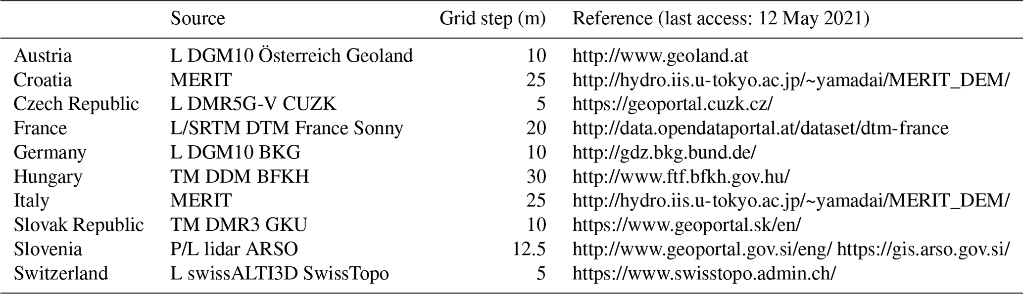
Each of these models was tested on a set of gravimetric points located at least 500 m from the border of each country. This test served both to detect possible artifacts in the DEMs (especially in high mountain areas) and also as a primary filter of the quality of the position of gravimetric points. These differences are illustrated in Fig. C1 and statistical findings in Table C2. Several points exceeding the threshold of ±50 m of difference between the measured and interpolated height were separately assessed and subsequently excluded from the database. The biggest differences are in Slovenia and the mountainous parts of France most likely due to the poor quality of station positions in old gravity data. Figure C2 presents the frequency distribution of the height residuals for the data sets of all contributing countries.
Table C2Statistical results of test calculations of consistency of surface station heights and DEMs used of the individual countries in the “most inner zone”.

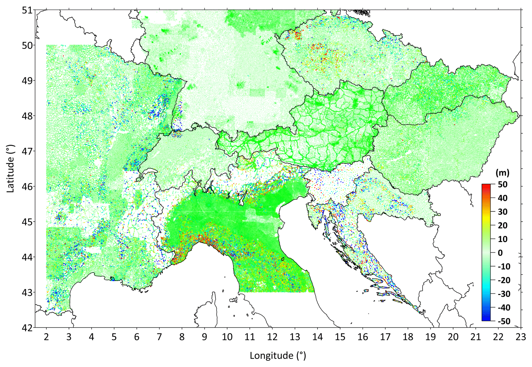
Figure C1Height differences (in meters) for DEMs in the “inner zone” of the TOPOSK software (refer to Appendix D) between the used DEMs and the heights of these stations.

Figure C2Histograms of height difference residuals of participating countries. The values in the different classes are given in meters.
For the calculation of MC within the middle zone (250–5240 m) it is very suitable to use DEMs with medium resolution (1–3 arcsec) which uniformly cover the whole territory, have the same shape representation and accuracy, and can be converted with local geoid and quasi-geoid models to ellipsoidal heights. Thanks to remote sensing satellite techniques, several commercial or freely available digital elevation models are currently available (https://insitu.copernicus.eu/library/reports/OverviewofGlobalDEM_i0r7.pdf, last access: 12 May 2021). We analyzed the most used and freely available models: Advanced Land Observing Satellite World 3D 30 m version 2.1 (AW3D30; Tadono et al., 2014; Takaku et al., 2018), Advanced Spaceborne Thermal Emission and Reflection Radiometer (ASTER) global digital elevation model version 3 (ASTER GDEM; NASA/METI/AIST/Japan Space Systems and U.S./Japan ASTER Science Team, 2020), NASA Shuttle Radar Topography Mission Global 1 arcsec (SRTMGL1; NASA JPL 2013), Multi-Error-Removed Improved-Terrain DEM (MERIT DEM; Yamazaki et al., 2017) and the digital elevation model over Europe version 1.1 (EU-DEM; EU-DEM, 2017). All models (Table C3) represent a digital surface model (with urban and canopy artifacts); only the MERIT model has partially removed vegetation and represents a mix of a digital surface and terrain model.
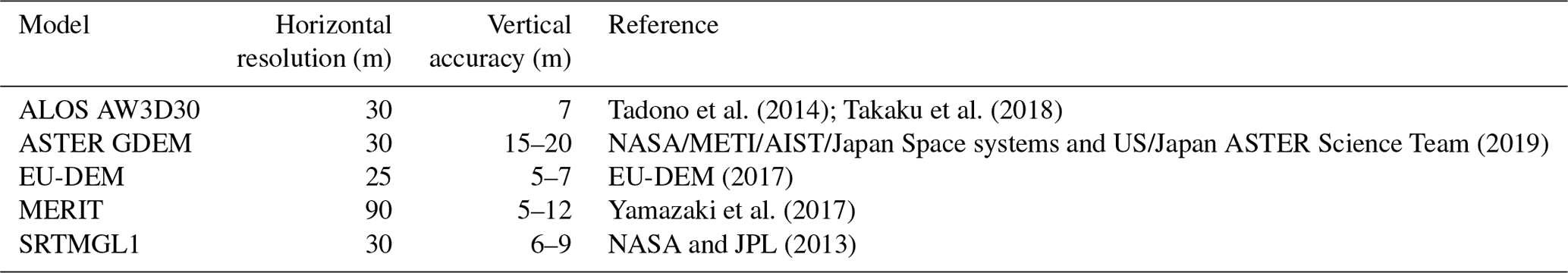
From these models the best one is MERIT due to the removal of major error components from the satellite DEMs like absolute biases, stripe, speckle noise and canopy height biases (Yamazaki et al., 2017; Hirt, 2018). This was confirmed also by an independent comparison at selected gravimetric points with new, precisely measured positions with GNSS in Switzerland, Slovenia and Slovakia (refer to Table C4 and Fig. C3), where large errors in the mountainous parts were due to canopy. The MERIT DEM was used in the original 3 arcsec resolution, and for T2 zone calculation it was resampled to the 25 m resolution.
The overall quality of the MERIT model has been tested at most gravity station heights. The differences can be seen in Fig. C4 and basic statistical data in Table C5.
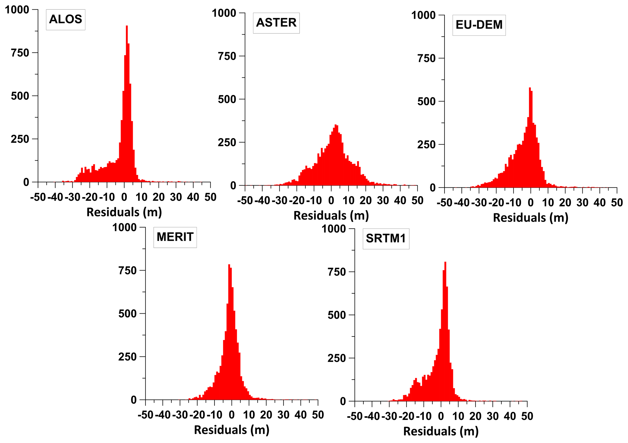
Figure C3Histograms of height residuals between global DEMs and 7097 selected gravity stations on the territory of Slovakia. The values in the different classes are given in meters.
Table C4Statistical results of test calculations of consistency of station heights for the territory of Slovakia (7097 points) and global DEMs tested.
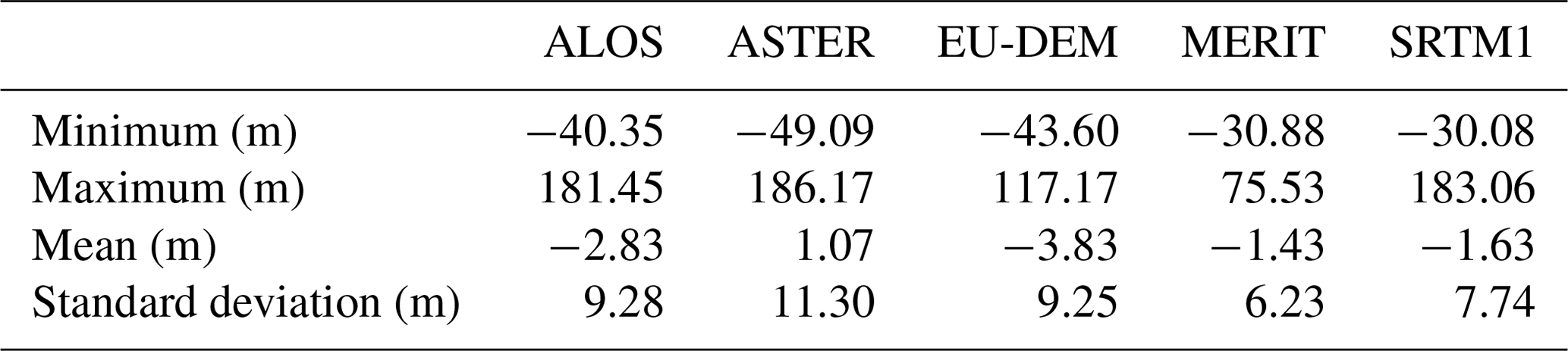
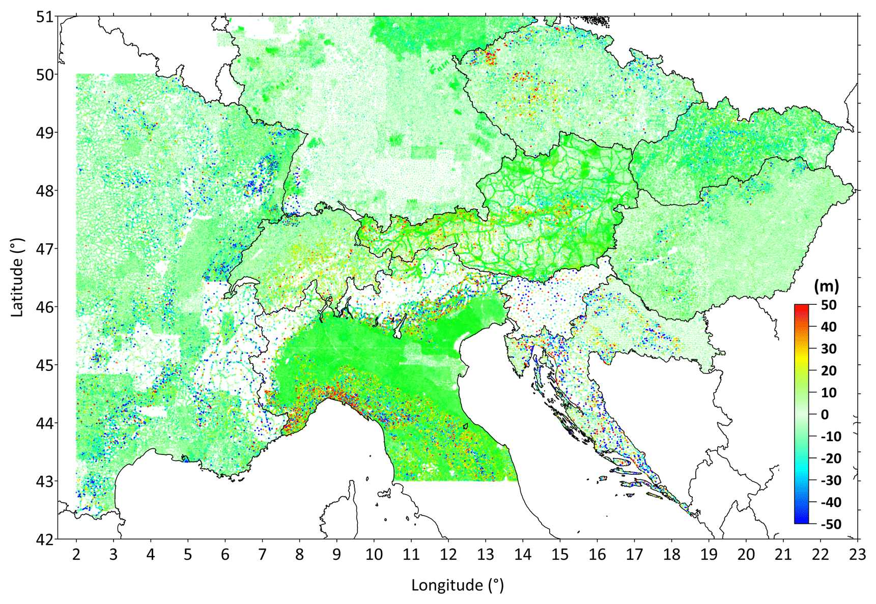
Figure C4Height differences (in meters) between MERIT DEM heights and heights of original surface-gravity stations; MERIT DEM heights were considered for the “middle zone” of the mass calculation software TOPOSK (refer to Appendix D).
Table C5Statistical results of test calculations of consistency of station heights and the MERIT DEM used.
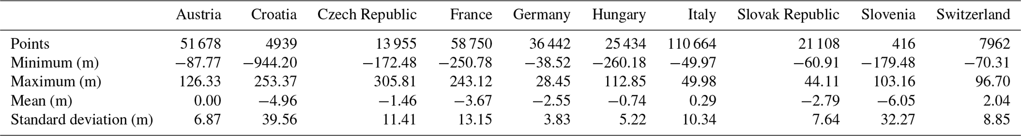
Largest differences were observed in Croatia, Czech Republic, France, and Hungary most likely due to the low quality of the position of gravity stations.
D1 The software test for calculations of mass correction
The Toposk software (Zahorec et al., 2017a) is designed for the calculation of the gravitational effect of the near-terrain masses for both “near-terrain effect” (NTE) and “mass correction” (MC), i.e., the total masses between the topography and the zero level – geoid or ellipsoid (we point out the difference from the terrain correction (TC), which represents only masses exceeding the classical “Bouguer shell”). The program is suitable for highly accurate calculations in rugged terrain using high-resolution DTMs. Different DTMs, with increasing resolution towards the calculation point, are used within particular zones. By default the program uses the following zoning:
-
T1: inner zone (0–250 m from the calculation point),
-
T2: intermediate zone (250–5240 m) and
-
outer zones: T31 (5.24–28.8 km) and T32 (28.8–166.7 km).
The standard outer limit of 166 730 m (equivalent to the spherical distance of 1∘ ) represents the outer limit of the zone O2 of the Hayford–Bowie system. Different analytic formulas are used within particular zones. The 3D polyhedral bodies are used within the inner zone. The planar approach is applied within the inner and intermediate zones, leading to a small negligible error with a maximum of a few tens of microgals for a density of 2670 kg m−3 (Zahorec et al., 2017a). The outer zones are treated by a spherical approach. By default, for the inner zone, the height used for the calculation of the correction at the position of the gravity station is interpolated from the DTM in order to reduce errors resulting from the height mismatch between point and DTM.
The TriTop software (Holzrichter et al., 2019) is an adaptive algorithm for MC based on a triangulated polyhedral representation of the topography. The runtime of the algorithm is improved by an automatic resampling of topography. The topography is resampled in a quadtree structure. The high resolution of the topography is only considered if it has a significant influence on the gravitational effect at the station and not only by the distance to the station. Therefore, there are no default zone radius definitions, but the resolution depends only on the gravitational effect and differs for each station. In comparison to Toposk, TriTop does not consider a high-resolution zone (T1; see above) and does not interpolate topography in this zone in dependence to station height. The DTM heights are not modified.
The programs were compared to each other on different sets of points from Slovakia and Austria. Mainly the second comparison was important because of the typical Alpine terrain character of the majority of the territory in Austria. The obtained results by the Toposk and TriTop software were compared with previously computed mass corrections (NTE) from the Austrian gravity database. This comparison was realized on a set of 28 420 points with the ellipsoidal heights ranging from 158.35 to 2898.78 m. The character of the differences between mass corrections from the Austrian gravity database and NTE calculations by means of the Toposk and TriTop programs is visible from histograms in Fig. D1. Finally, the Toposk software was selected for the recalculation of MC effects due to better statistical parameters (median and standard deviations) and the absence of outliers in the calculations. The differences in MC of both algorithms are observed in areas where stations are located close to steep slopes in topography. The differences of the results in Austria are caused by the main difference of both algorithms and in particular the handling of the inner zone T1. TriTop does not change or interpolate the topography around the station. This might lead to larger correction values in areas of highly rugged terrain due to steep slopes close to the station or even in cases in which the station height is slightly below the DTM. The comparison shows that in the area of highly rugged terrain the inner zone just around a station should be handled separately from the rest. Therefore, we decided to perform mass corrections with the Toposk software.
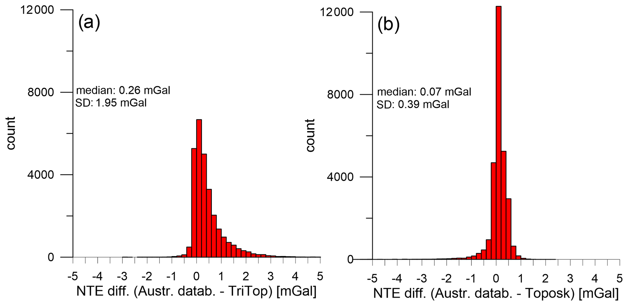
Figure D1Comparison of the differences between original mass corrections from the Austrian gravity database and NTE calculations by means of programs (a) TriTop and (b) Toposk.
D2 Comparison of mass corrections
For most countries, we used the available local detailed DEMs (Appendix C) with the resolution of 10–20 m (derived mainly from lidar data) for calculation in the innermost Toposk zone (T1). For all other zones we chose the best available global DEMs. We got good results with SRTM models for outer zones. For the intermediate zone T2, we decided to use the MERIT model based on our tests (Appendix C). MERIT was also used for the inner zone if local models were unavailable. This model (resampled to a 1 arcsec resolution) showed better height accuracy compared to other global models (based on the height residues at the points of the databases tested) and consequently minor differences in MC compared to local models (Fig. D2). The mentioned height residues of individual points of the databases in relation to local (or MERIT) models were subsequently used as a control criterion. In particular, we consider points with height residues greater than ±50 m to be untrustworthy, and they were excluded from the CBA compilation process. The following graphs and maps are compiled without these excluded points.
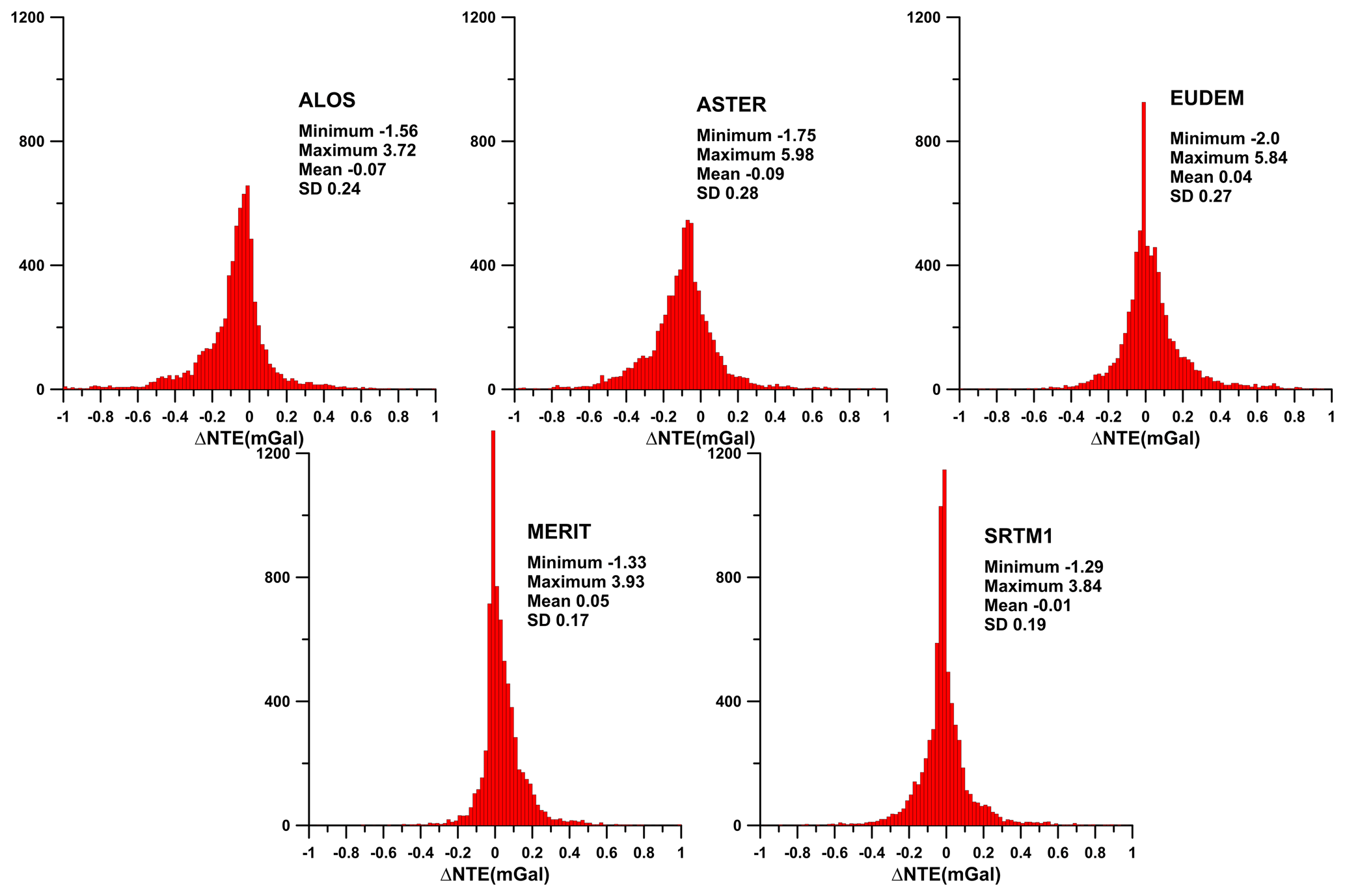
Figure D2Near-terrain effect (or mass correction, density 2670 kg m−3) differences calculated using various global models compared to the local Slovak terrain model DMR-3. The test was made on approx. 8000 points covering the whole territory of Slovakia.
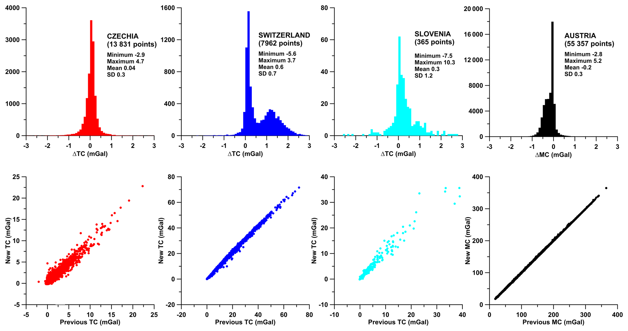
Figure D3Comparison of original mass correction (or terrain corrections) values and values calculated using local DEMs. Note: there are different scales for each graph.
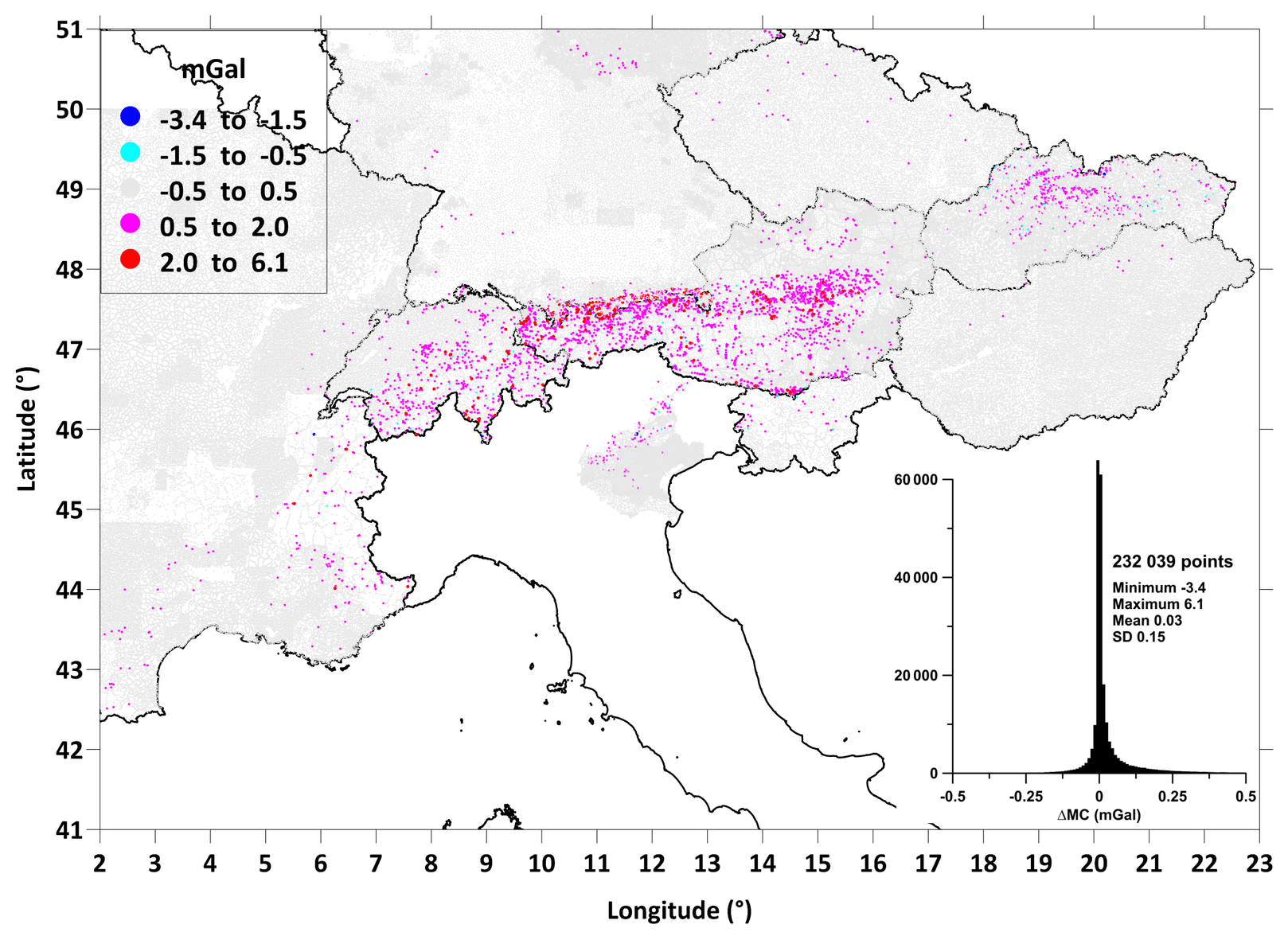
Figure D4Differences in mass correction values (correction density 2670 kg m−3) calculated by local DEMs which are derived mainly from lidar data and the MERIT model. For Italy, the part of the territory is displayed where for test reasons a local high-resolution DEM was used.
There are options to verify calculated MC values and estimate their error. For some databases, we had the original MC or TC values, which allows us to compare and control different approaches. Figure D3 shows graphs and statistical comparisons for some countries. The maximum differences are at the level of several milligals, and the RMS error in most cases is below 1 mGal. Note that the graphs do not show excluded points (above ±50 m height criterion), where significant differences in MC may be obtained. Another possibility to estimate the accuracy of the calculated MC is to compare the MC from the inner zone (where we can expect the most significant errors) for local DEMs and MERIT models. Figure D4 shows a map of these differences. The maximum differences are locally at the level of a few milligals and are mainly bound to mountain areas.
The supplement related to this article is available online at: https://doi.org/10.5194/essd-13-2165-2021-supplement.
While a separate page could be filled with detailed author contributions, we highlight the great joint effort that resulted in the current paper and, within that, that all authors contributed to data curation as the most crucial step.
The conceptualization stems from the AlpArray program and included authors GH, HJG, CB, RP, PZ, JP, MB, JE, GG, AG, BM, JS, PS, ES and MV.
The methodology and formal analysis rested mostly on the shoulders of PZ, JP, RP, BM, and CS for the processing of Mediterranean offshore data; there was help from many others, at least one person per country for investigating national data sets.
The original draft was written by HJG, BM, PZ, JP, MB, GH, RP, SB and CB. All co-authors have reviewed and approved the final version of the manuscript.
Funding was acquired on a national basis, as described in the acknowledgements.
HJG and GH ensured the overall project administration and supervision.
The authors declare that they have no conflict of interest.
This first compilation of gravity databases in the Alps and their surroundings has many helpers and supporters in the national administrations, state offices, national founding agencies, the academic working groups of the participating universities, the steering committee of the AlpArray program and finally in the library services of the GFZ (Potsdam, Germany). We would like to thank them all very much for their support. The group met several times for 2 d working meetings, and we gratefully thank the organizers. The results of this study contribute to the activities of EPOS (European Plate Observing System), its French component RESIF (Réseau Sismologique et Géodésique Français) and the Czech component CzechGeo. In Trieste (Italy) the research contributed to MIUR support for the Department of Mathematics and Geosciences, University of Trieste.
Finally, we would also like to thank Tomislav Bašić, Josip Stipčević (Croatia), Roland Pail, Reiner Rummel, Kirsten Elger, Christian Voigt (all from Germany), and an anonymous reviewer for supporting our work.
This research has been supported by EPOS/CzechGeo (grant no. LM-2015079), EPOS (European Plate Observing System), its French component RESIF (Réseau Sismologique et Géodésique Français), the German Research Foundation, (grant no. EB 255/7-1), the National Research, Development and Innovation Office, Hungary (grant no. 124241), the Swiss National Science Foundation (grant nos. PP00P2_157627, PP00P2_187199, and CRSII2_154434), the Slovak Research and Development Agency (grant nos. APVV 19-0150, APVV 16-0146, and APVV 16-0482), the Scientific Grant Agency VEGA, Slovakia (grant nos. 2/0006/19 and 2/0100/20), and the Slovenian Research Agency (grant no. P1-0011).
This paper was edited by Christian Voigt and reviewed by Roland Pail and one anonymous referee.
Allan, T. D. and Morelli, C.: A geological study of the Mediterranean Sea, Boll. Geofis. teor. appl., 13, 99–142, 1971.
Altamimi, Z.: EUREF Technical Note 1: Relationship and Transformation between the International and the European Terrestrial Reference Systems, Version June 28, available at: http://etrs89.ensg.ign.fr/pub/EUREF-TN-1.pdf (last access: 9 January 2021), 2018.
APAT: Gravity Map of Italy and Surrounding seas. 1:1 250 000, Agenzia per la protezione dell’ambiente e per I servizi tecnici, Dipartimento Difesa del Suolo, Servizio Geologico d'Italia, available at: https://www.isprambiente.gov.it/it/progetti/cartella-progetti-in-corso/suolo-e-territorio-1/cartografia-gravimetrica-digitale (last access: 13 May 2021), 2005.
Barzaghi, R., Borghi, A., Carrion, D., and Sona, G.: Refining the estimate of the Italian quasi-geoid, Bollettino di Geodesia e Scienze Affini, 66, 145–159, 2007.
Barzaghi, R., Carrion, D., Vergos, G. S., Tziavos, I. N., Grigoriadis, V. N., Natsiopoulos, D. A., Bruinsma, S., Reinquin, F., Seoane, L., Bonvalot, S., Lequentrec-Lalancette, M. F., Salaün, C., Andersen, O., Knudsen, P., Abulaitijiang, A., and Rio, M. H.: GEOMED2: High-Resolution Geoid of the Mediterranean, in: International Symposium on Advancing Geodesy in a Changing World – Proceedings of the IAG Scientific Assembly 2017, edited by: Sánchez, L. and Freymueller, J. T., 43–49, https://doi.org/10.1007/1345_2018_33, 2018.
Bašić, T.: Jedinstveni transformacijski model i novi model geoida Republike Hrvatske (Unique transformation model and new geoid model of the Republic of Croatia), available at: https://www.researchgate.net/publication/228791071_Jedinstveni_transformacijski_model_i_novi_model_geoida_Republike_Hrvatske_Unique_transformation_model_and_new_geoid_model_of_the_Republic_of_Croatia (last access: 18 February 2021), 2009.
Bašić, T. and Bjelotomic, O.: HRG2009: New High Resolution Geoid Model for Croatia, in: Gravity, Geoid and Height Systems, edited by: Martin, U., IAG Symposia Series, Springer Verlag, 187–191, https://doi.org/10.1007/978-3-319-10837-7_24, 2014.
Bielik, M., Kloska, K., Meurers, B., Švancara, J., and Wybraniec, S.: CELEBRATION 2000 Potential Field Working Group: Gravity anomaly map of the CELEBRATION 2000 region, Geologica Carpathica, 145–156, available at: http://www.geologicacarpathica.com/GeolCarp_Vol57_No3_145_156.html (last access: 11 February 2021), 2006.
Bilibajkič, P., Mladenovič, M., Mujagič, S., and Rimac, I.: Explanation for the gravity map of SFR Yugoslavia – Bouguer anomalies – 1:500 000, Federal Geological Institute Belgrade, Belgrade, 1 sheet, 1979.
Bomfim, E. P., Braitenberg, C., and Molina, E. C.: Mutual evaluation of global gravity models (EGM2008 and GOCE) and terrestrial data in Amazon Basin, Brazil, Geophys. J. Int., 195, 870–882, https://doi.org/10.1093/gji/ggt283, 2013.
Braitenberg, C., Ebbing, J., and Götze, H.-J.: Inverse modelling of elastic thickness by convolution method – the eastern Alps as an example, Earth Planet. Sc. Lett., 202, 387–404, https://doi.org/10.1016/S0012-821X(02)00793-8, 2002.
Braitenberg, C., Mariani, P., and De Min, A.: The European Alps and nearby orogenic belts sensed by GOCE, B. Geofis. Teor. Appl., 54, 321–334, https://doi.org/10.4430/bgta0105, 2013.
Bucha, B. and Janák, J.: A MATLAB-based graphical user interface program for computing functionals of the geopotential up to ultra-high degrees and orders, Comput. Geosci., 56, 186–196, https://doi.org/10.1016/j.cageo.2013.03.012, 2013.
Car, M., Gosar, A., Rajver, D., Stopar, R., and Tomšič, B.: History, state and perspectives of applied geophysics in Slovenia, Slovenian Association of Geodesy and Geophysics, Ljubljana, Slovenia, 43–86, 1996.
Cattin, R., Mazzotti, S., and Baratin, L.-M.: GravProcess: An easy-to-use MATLAB software to process campaign gravity data and evaluate the associated uncertainties, Comput. Geosci., 81, 20–27, https://doi.org/10.1016/j.cageo.2015.04.005, 2015.
Chapman, M. E. and Bodine, J. H: Consideration of the indirect effect in marine gravity modeling, J. Geophys. Res.-Sol. Ea., 84, 3889–3892, https://doi.org/10.1029/JB084iB08p03889, 1979.
Čibej, B.: Regional gravity map of Slovenia 1966–1967, Unpublished report, Geological Survey of Slovenia, Ljubljana, Slovenia, 1967 (in Slovenian).
Closs, H.: Die geophysikalische Reichsaufnahme und ihre Vorgeschichte, in: Zur Geschichte der Geophysik, Festschrift zur 50-jährigen Wiederkehr der Gründung der Deutschen Geophysikalischen Gesellschaft, edited by: Birett, H., Helbig, K., Kertz, W., and Schmucker, U., Springer, Berlin, Heidelberg, Germany, 115–130, https://doi.org/10.1007/978-3-642-65998-0_12, 2008.
C.N.R.-P.F.G.: Structural Model of Italy. Scale 1:500 000, Quaderni de “La Ricerca Scientifica”, CNR, 114, 1 map, 1992.
Cordell, L.: A scattered equivalent source method for interpretation and gridding of potential field data in three dimensions, Geophysics, 57, 629–636, https://doi.org/10.1190/1.1443275, 1992.
Csapó, G.: The Adjustment of the Hungarian Gravity Network in 2013, Az országos gravimetriai hálózat (MGH) 2013, évi kiegyenlítése és a hálózat megbízhatósági vizsgálata, Geodézia és Kartográfia, 65, https://www.mfttt.hu/mftttportal/index.php/geodezia-es-kartografia/tartalomjegyzek-2013/2013-11-12-65?jjj=1613062538677, (last access: 11 February 2021), 2013 (in Hungarian).
Csapó, G. and Koppán, A.: The results and works of the latest adjustment of Hungarian Gravimetric Network (MGH-2010), Acta Geod. Geophys., 48, 9–16, https://doi.org/10.1007/s40328-012-0001-5, 2013.
Csapó, G. and Völgyesi, L: Hungary's new gravity base network (MGH-2000) and its connection to the European Unified Gravity Net, in: Vistas for Geodesy in the New Millenium IAG Symposia, edited by: Ádám, J. and Schwarz, K. P., Springer, Berlin, Heidelberg, Germany, 72–77, https://doi.org/10.1007/978-3-662-04709-5_13, 2002.
Denker, H.: Regional gravity field modeling: Theory and practical results, in: Sciences of Geodesy – II, edited by: Xu, G., Springer, Berlin, Heidelberg, Germany, 185–291, https://doi.org/10.1007/978-3-642-28000-9_5, 2013.
Ebbing, J.: 3-D Dichteverteilung und isostatisches Verhalten der Lithosphäre in den Ostalpen, Dissertation, FB Geowissenschaften, FU Berlin, Germany, https://refubium.fu-berlin.de/handle/fub188/1302 (last access: 9 January 2021), 2002.
Ebbing, J., Braitenberg, C., and Götze, H.-J.: The lithospheric density structure of the Eastern Alps, Tectonophysics, 414, 145–155, https://doi.org/10.1016/j.tecto.2005.10.015, 2006.
Ehrismann, W., Rosenbach, O., and Steinhauser, P.: Untersuchungen zur Korrelation zwischen Freiluftanomalie und Stationshöhe im Hochgebirge, Österreichische Zeitschrift für Vermessung und Photogrammetrie, 57, 183–191, https://www.ovg.at/de/vgi/files/pdf/4108 (last access: 11 February 2021), 1969.
Ehrismann, W., Leppich, W., Lettau, O., Rosenbach, O., and Steinhauser, P.: Gravimetrische Detail-Untersuchungen in den westlichen Hohen Tauern, Z. Geophys., 39, 115–130, https://doi.org/10.23689/fidgeo-3180, 1973.
Ehrismann, W., Götze, H.-J., Leppich, W., Lettau, O., Rosenbach, O., Schöler, W., and Steinhauser, P.: Gravimetrische Feldmessungen und Modellberechnungen im Gebiet des Krimmler Ache Tales und des Obersulzbachtales (Groß Venedigergebiet/Österreich), Geol. Rundsch., 65, 767–778, https://doi.org/10.1007/BF01808493, 1976.
EMODnet Bathymetry Consortium: EMODnet Digital Bathymetry (DTM), available at: https://doi.org/10.12770/18ff0d48-b203-4a65-94a9-5fd8b0ec35f6, 2018.
EU-DEM: EU-DEM digital surface model v1.1, available at: https://www.eea.europa.eu/data-and-maps/data/copernicus-land-monitoring-service-eu-dem (last access: 9 January 2021), 2017.
Ferri, F., Ventura, R., Coren, F., and Zanolla, C.: Gravity map of italy and surrounding seas, Carta Gravimetrica d'Italia, 1:1 250 000, APAT Agenzia per la protezione dell'ambiente e per i servizi tecnici, Rome, Italy, 2005.
Förste, C., Bruinsma, S. L., Abrikosov, O., Lemoine, J.-M., Marty, J. C., Flechtner, F., Balmino, G., Barthelmes, F., and Biancale, R.: EIGEN-6C4 – The latest combined global gravity field model including GOCE data up to degree and order 2190 of GFZ Potsdam and GRGS Toulouse GFZ Data Services, available at: https://doi.org/10.5880/icgem.2015.1 (last access: 13 May 2021), 2014.
Francis, O., Baumann, H., Ullrich, C., Castelein, S., Van Camp, M., de Sousa, M. A., Lima Melhorato, R., Li, C., Xu, J., Su, D., Wu, S., Hu, H., Wu, K., Li, G., Li, Z., Hsieh, W.-C., Pálinkás, P. V., Kostelecký, J., Mäkinen, J., Näränen, J., Merlet, S., Pereira Dos Santos, F., Gillot, P., Hinderer, J., Bernard, J.-D., Le Moigne, N., Fores, B., Gitlein, O., Schilling, M., Falk, R., Wilmes, H., Germak, A., Biolcati, E., Origlia, C., Iacovone, D., Baccaro, F., Mizushima, S., De Plaen, R., Klein, G., Seil, M., Radinovic, R., Sekowski, M., Dykowski, P., Choi, I.-M., Kim, M.-S., Borreguero, A., Sainz-Maza, S., Calvo, M., Engfeldt, A., Agren, J., Reudink, R., Eckl, M., van Westrum, D., Billson, R., and Ellis, B.: CCM.G-K2 key comparison, Metrologia, 52, 07009, https://doi.org/10.1088/0026-1394/52/1A/07009, 2015.
GEBCO Compilation Group: GEBCO_2020 Grid, National Oceanography Centre, British Oceanographic Data Centre, Liverpool, United Kingdom, https://doi.org/10.5285/a29c5465-b138-234d-e053-6c86abc040b9 (last access: 13 May 2021), 2020.
Gerke, K.: Die Karte der Bouguer-Isanomalen, 1V1 000 000 von Westdeutschland, Deutsche Geodätische Kommission der Bayerischen Akademie der Wissenschaften/Reihe B: Angewandte Geodäsie, Frankfurt a. M., 1957.
Gosar, A.: Mohorovičić discontinuity depth, in: Geological atlas of Slovenia, edited by: Novak, M. and Rman, N., Geological Survey of Slovenia, Ljubljana, Slovenia, 18–19, 2016.
Götze, H.-J.: Ein numerisches Verfahren zur Berechnung der gravimetrischen Feldgrößen dreidimensionaler Modellkörper, Arch. Meteor. Geophy. A, 25, 195–215, 1978.
Götze, H.-J. and Lahmeyer, B.: Application of three-dimensional interactive modelling in gravity and magnetics, Geophysics, 53, 1096–1108, https://doi.org/10.1190/1.1442546, 1988.
Götze, H.-J., Rosenbach, O., and Schöler, W.: Gravimetric measurements on three N-S profiles through the Eastern Alps – Observational results and preliminary modeling, in: Alps, Apennines, Hellenides, edited by: Closs, H., Roeder, D., Schmidt, K., Inter-Union Comm. on Geodynamics, Scient. Report 38, E. Schweizerbartsche Verlagsbuchhandlung, Stuttgart, Germany, 44–49, 1978.
Götze, H.-J., Rosenbach, O., and Schöler, W.: Gravimetrische Untersuchungen in den östlichen Zentralalpen, Geol. Rundsch., 68, 61–82, https://doi.org/10.1007/BF01821122, 1979.
Götze, H.-J., Meurers, B., Schmidt, S., and Steinhauser, P.: On the isostatic state of the Eastern Alps and the Central Andes – a statistical comparison, in: Andean Magmatism and its Tectonic Setting, edited by: Harmon, R. S. and Rapela, C. W., Geol. S. Am. S., 265, 279–290, ISBN 0813722659, 9780813722658, 1991.
Grand, A.: Reconstruction of complete Bouguer anomalies maps from archive records and their use in practice, Diploma thesis, Comenius University, Bratislava, Slovakia, 2019.
Grand, T., Šefara, J., Pašteka, R., Bielik, M., and Daniel, S.: Atlas of geophysical maps and profiles, Part D1: gravimetry, Final report, MS Geofond State Geological Institute, Bratislava, Slovakia, 2001 (in Slovak).
Grandjean, G., Mennechet, C., Debeglia, N., and Bonijoly, D.: Insuring the quality of gravity data, Eos Transactions, 79, 217–221, 1998.
Guglielmetti, L., Comina, C., Abdelfettah, Y., Schill, E., and Mandrone, G.: Integration of 3D geological modeling and gravity surveys for geothermal prospection in an Alpine region, Tectonophysics, 608, 1025–1036, https://doi.org/10.1016/j.tecto.2013.07.012, 2013.
Hackney, R. I. and Featherstone, W. E.: Geodetic versus Geophysical Perspectives of the “Gravity Anomaly”, Geophys. J. Int., 154, 35–43, https://doi.org/10.1046/j.1365-246X.2003.01941.x, 2003.
Handy, M. R., Schmid, S. M., Bousquet, R., Kissling, E., and Bernoulli, D.: Reconciling plate-tectonic reconstructions of Alpine Tethys with the geological-geophysical record of spreading and subduction in the Alps, Earth-Sci. Rev., 102, 121–158, https://doi.org/10.1016/j.earscirev.2010.06.002, 2010.
Harpha Sea: Bathymetric data for Bohinj and Bled lakes, Unpublished report, Aljoša Žerjal, Harpha Sea, d.o.o. Koper, 2017.
Heiskanen, W. A. and Moritz, H.: Physical geodesy, W. H. Freeman Co, https://doi.org/10.1017/S0016756800048834 (last access: 13 May 2021), 1967.
Hetényi, G., Cattin, R., Berthet, T., Le Moigne, N., Chophel, J., Lechmann, S., Hammer, P., Drukpa, D., Sapkota S. N., Gautier S., and Thinley, K.: Segmentation of the Himalayas as revealed by arc-parallel gravity anomalies, Sci. Rep.-UK, 6, 33866, https://doi.org/10.1038/srep33866, 2016.
Hetényi, G., Molinari, I., Clinton, J., Bokelmann, G., Bondár, I., Crawford, W. C., Dessa, J.-X., Doubre, C., Friederich, W., Fuchs, F., Giardini, D., Gráczer, Z., Handy, M. R., Herak, M., Jia, Y., Kissling, E., Kopp, H., Korn, M., Margheriti, L., Meier, T., Mucciarelli, M., Paul, A., Pesaresi, D., Piromallo, C., Plenefisch, T., Plomerová, J., Ritter, J., Rümpker, G., Šipka, V., Spallarossa, D., Thomas, C., Tilmann, F., Wassermann, J., Weber, M., Wéber, Z., Wesztergom, V., Živčić, M., AlpArray Seismic Network Team, AlpArray OBS Cruise Crew, and AlpArray Working Group: A Large-Scale European Experiment to Image the Alpine Orogen, Surv. Geophys., 39, 1009–1033, https://doi.org/10.1007/s10712-018-9472-4, 2018.
Hirt, C.: Artefact detection in global digital elevation models (DEMs): The Maximum Slope Approach and its application for complete screening of the SRTM v4.1 and MERIT DEMs, Remote Sens. Environ., 207, 27–41, https://doi.org/10.1016/j.rse.2017.12.037, 2018.
Holzrichter, N., Szwillus, W., and Götze, H.-J.: An adaptive topography correction method of gravity field and gradient measurements by polyhedral bodies, Geophys. J. Int., 218, 1057–1070, https://doi.org/10.1093/gji/ggz211, 2019.
IGN: Descriptifs quasi-geoides et grilles de conversion altimétrique sur la France métropolitaine, Laboratoire de Recherche en Géodésie, Service de Geodesie et Nivellement, available at: https://geodesie.ign.fr/contenu/fichiers/GrillesConversionAltimetrique.pdf (last access: 11 February 2021), 2010.
Kahle, H. G. and Klingelé, E.: Recent activities in gravimetry and physical geodesy, Schweiz. Miner. Petrog., 59, 207–217, 1979.
Karcol, R.: Gravitational attraction and potential of spherical shells with radially dependent density, Stud. Geophys. Geod., 55, 21–34, https://doi.org/10.1007/s11200-011-0002-9, 2011.
Kissling, E.: Krustenaufbau und Isostasie in der Schweiz, Dissertation Nr. 6655, ETH Zurich, Zurich, Switzerland, 167 pp., available at: https://docplayer.org/78935193-Krustenaufbau-und-isostasie-in-der-schweiz.html (last access: 9 January 2021), 1980.
Klingelé, E. and Olivier, R.: Die neue Schwerekarte der Schweiz (Bouguer Anomalien), Géophysique, No. 20, Swiss Geophysical Commission, Bern, 93 pp., 1 map, 1980.
Kostelecky, J., Kostelecky Jr., J., Pesek, I., Simek, J., Svabensky, O., Weigel, J., and Zeman, A.: Quasi Geoid for the Territory of the Czech Republic, Stud. Geophys. Geod., 48, 503–518, https://doi.org/10.1023/B:SGEG.0000037469.70838.39, 2004.
Kuhar, M., Berk, S., Koler, B., Medved, K., Omang, O., and Solheim, D.: Vloga kakovostnega višinskega sistema in geoida za izvedbo GNSS-višinomerstva, The quality role of height system and geoid model in the realization of GNSS heighting, Geod. Vestn., 55, 226–234, https://doi.org/10.15292/geodetski-vestnik.2011.02.226-234, 2011 (in Slovenian).
Leibniz-Institut für Angewandte Geophysik: Schwerekarte der Bundesrepublik Deutschland 1:1 000 000 Bouguer-Anomalien, Leibniz-Institut für Angewandte Geophysik, Hannover, Germany, 2010.
Lequentrec-Lalancette, M. F., Salaun, C., Bonvalot, S., Rouxel, D., and Bruinsma, S.: Exploitation of Marine Gravity Measurements of the Mediterranean in the Validation of Global Gravity Field Models, in: International Symposium on Earth and Environmental Sciences for Future Generations, International Association of Geodesy Symposia, Prague, Czech Republic, 22 June–2 July 2015, 63–67, https://doi.org/10.1007/1345_2016_258 (last access: 13 May 2021), 2016.
Li, X. and Götze, H.-J.: Ellipsoid, geoid, gravity, geodesy and geophysics, Geophysics, 66, 1660–1668, https://doi.org/10.1190/1.1487109, 2001.
Marson, I. and Klingelé, E.: Advantages of using the vertical gradient of gravity for 3-D interpretation, Geophysics, 58, 1588, https://doi.org/10.1190/1.1443374, 1993.
Martelet, G., Pajot, G., and Debeglia, N.: Nouvelle carte gravimétrique de la France, RCGF09 – Réseau et Carte Gravimétrique de la France, Rapport BRGM/RP-57908-FR, available at: http://infoterre.brgm.fr/rapports/RP-57908-FR.pdf (last access: 11 February 2021), 2009.
Marti, U.: Comparison of high precision geoid models in Switzerland, in: Dynamic Planet: Monitoring and Understanding a Dynamic Planet with Geodetic and Oceanographic Tools, edited by: Tregonig, P. and Rizos, C., IAG Symposia Series, Springer, Berlin, Heidelberg, Germany, 377–382, https://doi.org/10.1007/978-3-540-49350-1_55, 2007.
Meurers, B.: Bearbeitung der Schweredaten der OMV-AG, Unpublished report OMV-AG, Vienna, Austria, 1992a.
Meurers, B.: Untersuchungen zur Bestimmung und Analyse des Schwerefeldes im Hochgebirge am Beispiel der Ostalpen, Österreichische Beiträge zu Meteorologie und Geophysik, ZAMG Publ. Nr. 343, Vienna, Austria, 146 pp., 1992b.
Meurers, B.: The Physical Meaning of Bouguer Anomalies – General Aspects Revisited, in: Understanding the Bouguer Anomaly – A Gravimetry Puzzle, edited by: Pašteka, R., Meurers, B., and Mikuška, J., Elsevier, Amsterdam, The Netherlands, 13–30, https://doi.org/10.1016/B978-0-12-812913-5.00001-4, 2017.
Meurers, B. and Ruess, D.: Compilation of a new Bouguer gravity data base in Austria, in: Austrian Contributions to IUGG 2007, Perugia, Italy, edited by: Brunner, F., Kahmen, H., and Schuh, H., Österreichische Zeitschrift für Vermessung und Geoinformation, 95, 90–94, https://www.ovg.at/de/vgi/files/pdf/4959 (last access: 11 February 2021), 2007.
Meurers, B. and Ruess, D.: A new Bouguer gravity map of Austria, Austrian J. Earth Sc., 102, 62–70, https://www.univie.ac.at/ajes/archive/volume_102_1/meurers_ruess_ajes_v102_1.pdf (last access: 23 February 2021), 2009.
Meurers, B., Ruess, D., and Steinhauser, P.: The Gravimetric Alpine Traverse, in: Geodynamics of the Eastern Alps, edited by: Flügel, H. and Faupl, P., Deuticke, Vienna, Austria, 334–344, 1987.
Meurers, B., Ruess, D., and Graf, J.: A program system for high precise Bouguer gravity determination, in: Proc. 8th International Meeting on Alpine Gravimetry, Österreichische Beiträge zu Meteorologie und Geophysik, edited by: Meurers, B., 217–226, 2001.
Mikuška, J., Pašteka, R., and Marušiak, I.: Estimation of distant relief effect in gravimetry, Geophysics, 71, 59–69, https://doi.org/10.1190/1.2338333, 2006.
Mikuška, J., Marušiak, I., Pašteka, R., Karcol, R., and Beňo, J.: The effect of topography in calculating the atmospheric correction in gravimetry, in: 2008 SEG Annual Meeting, Las Vegas, Nevada, USA, 9–14 November 2008, 784–788, available at: https://onepetro.org/SEGAM/proceedings/SEG08/All-SEG08/SEG-2008-0784/94539 (last access: 13 May 2021), 2008.
Morelli, C.: Discussione e considerazioni sulla compensazione d'insieme della rete internazionale delle stazioni di riferimento per le misure di gravità relativa, Ann. Geophys.-Italy, 1, 425–454, https://doi.org/10.4401/ag-6076, 1948.
Morelli, C., Gantar, C., Honkasalo, T., McConnell, R. K., Tanner, I. G., Szabo, B., Uotila, U., and Whalen, C. T.: The International Gravity Standardisation Net 1971 (IGSN71), IAG, Spec. Publ., 4, Paris, France, available at: https://apps.dtic.mil/dtic/tr/fulltext/u2/a006203.pdf (last access: 13 May 2021), 1972.
Moritz, H.: Geodetic reference system 1980, B. Geod., 54, 395–405, https://doi.org/10.1007/BF02521480, 1984.
Moritz, H.: Geodetic Reference System 1980, J. Geodesy, 74, 128–133, https://doi.org/10.1007/s001900050278, 2000.
NASA JPL: NASA Shuttle Radar Topography Mission Global 1 arc second [Data set], NASA EOSDIS Land Processes DAAC, available at: https://doi.org/10.5067/MEaSUREs/SRTM/SRTMGL3S.003, 2013.
NASA/METI/AIST/Japan Space systems and U.S./Japan ASTER Science Team, ASTER Global Digital Elevation Model V003, NASA EOSDIS Land Processes DAAC, available at: https://doi.org/10.5067/ASTER/ASTGTM.003, 2019.
Niethammer, T.: Schwerebestimmungen in den Jahren 1915–1918, Astronomisch-geodätische Arbeiten in der Schweiz, Schweizerische geodätische Kommission, Bern, 16, 1–219, 1921.
Olivier, R., Dumont, B., and Klingelé, E.: L’Atlas Gravimétrique 85 de la Suisse, Swiss Geophysical Commission, Bern, 43, 62 pp., 22 maps, 2010.
Oncken, O., Chong, G., Franz, G., Giese, P., Götze, H.-J., Ramos, V. A., Strecker, M. R., and Wigger, P.: The Andes: active subduction orogeny, Springer, Berlin, Heidelberg, Germany, ISBN-13978-3-540-24320-8, https://doi.org/10.1007/978-3-540-48684-8, 2006.
Pail, R., Kühtreiber, N., Wiesenhofer, B., Hofmann-Wellenhof, B., Steinbach, O., Höggerl, N., Imrek, E., Ruess, D., and Ullrich, C.: The Austrian Geoid 2007, Österreichische Zeitschrift für Vermessung und Geoinformation, 96, 3–14, https://www.ovg.at/de/vgi/ausgabe/1249/#article4983 (last access: 13 May 2021), 2008.
Pašteka, R., Mikuska, J., and Meurers, B.: Understanding the Bouguer Anomaly: A Gravimetry Puzzle, Elsevier, Amsterdam, The Netherlands, ISBN: 978-0-12-812913-5, 2017.
Pavlis, N. K., Factor, J. K., and Holmes, S. A.: Terrain-related gravimetric quantities computed for the next EGM, in: Proceedings of the 1st International Symposium of the International Gravity Field Service, Harita Dergisi, Istanbul, 318–323, 2007.
Pavlis, N. K., Holmes, S. A., Kenyon, S. C., and Factor, J. K.: The development and evaluation of the Earth Gravitational Model 2008 (EGM2008), J. Geophys. Res.-Sol. Ea., 117, B04406, https://doi.org/10.1029/2011JB008916, 2012.
Pistone, M., Müntener, O., Ziberna, L., Hetényi, G., and Zanetti, A.: Report on the ICDP workshop DIVE (Drilling the Ivrea–Verbano zonE), Sci. Dril., 23, 47–56, https://doi.org/10.5194/sd-23-47-2017, 2017.
Pivetta, T. and Braitenberg, C.: Sensitivity of gravity and topography regressions to earth and planetary structures, Tectonophysics, Tectonophysics, 774, 228–299, https://doi.org/10.1016/j.tecto.2019.228299, 2020.
Plaumann, S.: Die Schwerekarte 1:500 000 der Bundesrepublik Deutschland (Bouguer Anomalien), Blatt Süd, Geologisches Jahrbuch, E 53, 1–13, Hannover, 1995.
Posch, E. and Walach, G.: Das Bouguer Schwerefeld in Vorarlberg und im Bereich der Übergangszone zwischen West- und Ostalpen, in: Tagungsbericht über das 5. Int. Alpengravimetrie Kolloquium, Graz, Austria, 1989, Österreichische Beiträge zu Meteorologie und Geophysik, edited by: Lichtenegger, H., Steinhauser, P., and Sünkel, H., ZAMG Publ. Nr. 332, Vienna, Austria, 147–151, 1990.
Ravnik, D., Stopar, R., Car, M., Živanović, M., Gosar, A., Rajver, D., and Andjelov, M.: Results of applied geophysical investigations in Slovenia, Slovenian Association of Geodesy and Geophysics, Ljubljana, Slovenia, 49–67, 1995.
Ruess, D.: Der Beitrag Österreichs an UNIGRACE – Unification of Gravity Systems of Central and Eastern European Countries, Österreichische Zeitschrift für Vermessung und Geoinformation, 90, 129–139, https://www.ovg.at/de/vgi/ausgabe/1230/#article4853 (last access: 11 February 2021), 2002.
Scarponi, M., Hetényi, G., Berthet, T., Baron, L., Manzotti, P., Petri, B., Pistone, M., and Müntener, O.: New gravity data and 3D density model constraints on the Ivrea Geophysical Body (Western Alps), Geophys. J. Int., 222, 1977–1991, https://doi.org/10.1093/gji/ggaa263, 2020.
Schmidt, S.: Untersuchungen zum regionalen Verlauf des Vertikalgradienten der Schwere im Hochgebirge, Ph.D. thesis, Technische Universität Clausthal, Clausthal, Germany, 1985.
Schwabe, J., Liebsch, G., and Schirmer, U.: Refined computation strategies for the new German Combined Quasigeoid GCG2016, in: Symposium on Geoid, Gravity and Height Systems (GGHS2016), Thessaloniki, Greece, 19–23 September 2016.
Senftl, E.: Schwerekarte von Österreich, Bouguer-Isanomalen 1:1 000 000, Bundesamt für Eich- und Vermessungswesen, Vienna, Austria, 1965.
Shahrokh, P., Emery, X., and Madani, N.: Comparing sequential Gaussian and turning bands algorithms for cosimulating grades in multi-element deposits, C. R. Geosci., 347, 84–93, https://doi.org/10.1016/j.crte.2015.05.008, 2015.
Skiba, P.: Homogene Schwerekarte der Bundesrepublik Deutschland (Bouguer-Anomalien), Technischer Bericht zur Fortführung der Datenbasis, deren Auswertung und Visualisierung, LIAG-Bericht, Hannover, Germany, 89 pp., available at: https://doi.leibniz-liag.de/doi.php?obj=rep-12346-1 (last access: 31 May 2021), 2011.
Somigliana, C.: Teoria generale del campo gravitazionale dell' ellipsoide di rotazione, Mem. Soc. Astron Ital., 4, 425, 1929.
Steinhauser, P., Meurers, B., and Ruess, D.: Gravity investigations in mountainous areas, Explor. Geophys., 21, 161–168, https://doi.org/10.1071/EG990161, 1990.
Stopar, R.: Map of the Bouguer anomalies, in: Geological atlas of Slovenia, edited by: Novak, M. and Rman, N., Geological Survey of Slovenia, Ljubljana, Slovenia, 20–21, 2016.
Surveying and mapping authority of Slovenia: Digital elevation models for Slovenia in 12.5 and 25 m grid size, available at: https://www.e-prostor.gov.si/access-to-geodetic-data/ordering-data/ (last access: 9 January 2021), 2019.
Szabó, Z.: The history of the 125 year old Eötvös torsion balance, Acta Geod. Geophys., 51, 273–293, https://doi.org/10.1007/s40328-015-0126-4, 2016.
Szwillus, W., Ebbing, J., and Holzrichter, N.: Importance of far-field Topographic and Isostatic corrections for regional density modelling, Geophys. J. Int., 207, 274–287, https://doi.org/10.1093/gji/ggw270, 2016.
Tadiello, D. and Braitenberg, C.: Gravity modeling of the Alpine lithosphere affected by magmatism based on seismic tomography, Solid Earth, 12, 539–561, https://doi.org/10.5194/se-12-539-2021, 2021.
Tadono, T., Ishida, H., Oda, F., Naito, S., Minakawa, K., and Iwamoto, H.: Precise Global DEM Generation By ALOS PRISM, ISPRS-Annals of the Photogrammetry, Remote Sensing and Spatial Information Sciences, 4, 71–76, https://doi.org/10.5194/isprsannals-II-4-71-2014, 2014.
Takaku, J., Tadono, T., Tsutsui, K., and Ichikawa, M.: Quality Improvements of “AW3D” Global DSM Derived from ALOS PRISM, in: Proc. the 38th annual symposium of the IEEE Geoscience and Remote Sensing Society (IGARSS2018), Valencia, Spain, 22–27 July 2018, 1612–1615, 2018.
Varga, M.: The Application of Crustal Models in Regional Modelling of the Earth's Gravity Field (PhD thesis), Faculty of Geodesy, University of Zagreb, Zagreb, Croatia, https://doi.org/10.13140/RG.2.2.11800.08963/2, 2018.
VITEL: http://geomentor.hu/VITEL_TRF (last access: 11 February 2021), 2020.
Walach, G.: The Gravity Field in Southern Austria, Mitteilungen des Geodätischen Instituts der Technischen Universität Graz, Graz, Austria, 135–140, 1990.
Wenzel, H.: Hochauflösende Kugelfunktionsmodelle für das Gravitationspotential der Erde, Wissenschaftliche Arbeiten der Fachrichtung Vermessungswesen der Universität Hannover, Hannover, Germany, 1985.
Winter, P.: Die Karte der Bouguer-Isanomalen der Steiermark und benachbarter Gebiete, in: Tagungsbericht über das 6. Int. Alpengravimetriekolloquium, Österreichische Beiträge zu Meteorologie und Geophysik, edited by: Steinhauser, P. and Walach, G., ZAMG Publ. Nr. 353, Vienna, Austria, 55–68, 1993.
Wollard, G. P.: New Gravity System – Changes in International Gravity Base Values and Anomaly Values, Geophysics, 44, 1352–1366, https://doi.org/10.1190/1.1441012, 1979.
Yamazaki, D., Ikeshima, D., Tawatari, R., Yamaguchi, T., O'Loughlin, F., Neal, J. C., Sampson, C. C., Kanae, S., and Bates, P. D.: A high accuracy map of global terrain elevations, Geophys. Res. Lett., 44, 5844–5853, https://doi.org/10.1002/2017GL072874, 2017.
Zahorec, P., Marušiak, I., Mikuška, J., Pašteka, R., and Papčo, J.: Numerical calculation of terrain correction within the Bouguer anomaly evaluation (program Toposk), in: Understanding the Bouguer Anomaly – A Gravimetry Puzzle, edited by: Pašteka, R., Mikuška, J., and Meurers, B., Elsevier, Amsterdam, The Netherlands, 79–92, https://doi.org/10.1016/B978-0-12-812913-5.00004-X, 2017a.
Zahorec, P., Pašteka, R., Mikuška, J., Szalaiová, V., Papčo, J., Kušnirák, D., Pánisová, J., Krajňák, M., Vajda, P., Bielik, M., and Marušiak, I.: National Gravimetric Database of the Slovak Republic, in: Understanding the Bouguer Anomaly – A Gravimetry Puzzle, edited by: Pašteka, R., Mikuška, J., and Meurers, B., Elsevier, Amsterdam, The Netherlands, 113–125, https://doi.org/10.1016/B978-0-12-812913-5.00004-X, 2017b.
Zahorec, P., Papčo, J., Pašteka, R., Bielik, M., Bonvalot, S., Braitenberg, C., Ebbing, J., Gabriel, G., Gosar, A., Grand, A., Götze, H.-J., Hetényi, G., Holzrichter, N., Kissling, E., Marti, U., Meurers, B., Mrlina, J., Nogová, E., Pastorutti, A., Salaun, C., Scarponi, M., Sebera, J., Seoane, L., Skiba, P., Szűcs, E., and Varga, M.: The Pan-Alpine gravity database 2020, GFZ Data Services, available at: https://doi.org/10.5880/fidgeo.2020.045, 2021.
ZBGIS: Geoportál, available at: https://www.geoportal.sk/sk/sluzby/aplikacie/mapovy-klient-zbgis/ (last access: 18 February 2021), 2020.
Zych, D.: 30 Jahre Gravimetermessungen der ÖMV Aktiengesellschaft in Österreich und ihre geologisch-geophysikalische Interpretation, Archiv für Lagerstättenforschung, Geologische Bundesanstalt, Vienna, Austria, 155–175, 1988.
Note: though different from the SI units, we will use the unit mGal for gravity, which is still frequently used in gravimetry; 1 mGal = 10−5 m s−2.
- Abstract
- Introduction
- Assessment of database
- Reprocessing of original data and applied corrections
- The new homogenized gravity maps for the Alps
- Uncertainties of data and map
- Availability of the digital data sets and criteria of use
- Data availability
- Conclusions
- Appendix A: Abbreviations
- Appendix B: Historical remarks on Alpine gravity surveys and national gravity databases for AAGRG Bouguer gravity compilation
- Appendix C: Digital elevation models in the AlpArray region
- Appendix D: Mass correction – software and comparisons
- Author contributions
- Competing interests
- Acknowledgements
- Financial support
- Review statement
- References
- Supplement