Last interglacial (MIS 5e) sea-level proxies in southeastern South America

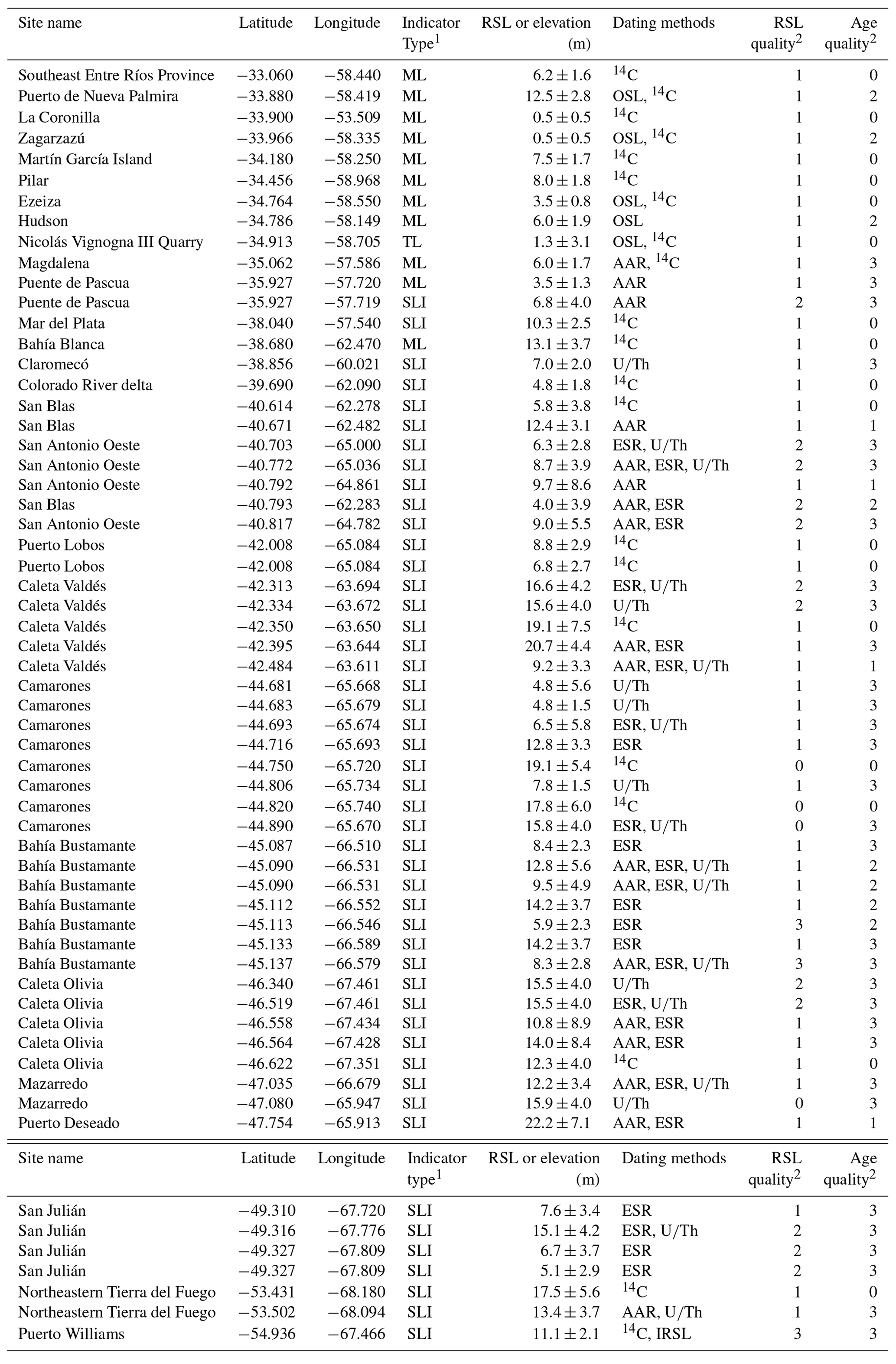
Coastal southeast South America is one of the classic locations where there are robust, spatially extensive records of past high sea level. Sea-level proxies interpreted as last interglacial (Marine Isotope Stage 5e, MIS 5e) exist along the length of the Uruguayan and Argentinian coast with exceptional preservation especially in Patagonia. Many coastal deposits are correlated to MIS 5e solely because they form the next-highest terrace level above the Holocene highstand; however, dating control exists for some landforms from amino acid racemization, U∕Th (on molluscs), electron spin resonance (ESR), optically stimulated luminescence (OSL), infrared stimulated luminescence (IRSL), and radiocarbon dating (which provides minimum ages). As part of the World Atlas of Last Interglacial Shorelines (WALIS) database, we have compiled a total of 60 MIS 5 proxies attributed, with various degrees of precision, to MIS 5e. Of these, 48 are sea-level indicators, 11 are marine-limiting indicators (sea level above the elevation of the indicator), and 1 is terrestrial limiting (sea level below the elevation of the indicator). Limitations on the precision and accuracy of chronological controls and elevation measurements mean that most of these indicators are considered to be low quality. The database is available at https://doi.org/10.5281/zenodo.3991596 (Gowan et al., 2020).

1 Database and literature overview

During Marine Isotope Stage (MIS) 5e (about 130–115 ka), global sea level was 5–9 m higher than at present (Kopp et al., 2009; Dutton and Lambeck, 2012; Rovere et al., 2016). MIS 5e represents one substage within MIS 5 (about 130–71 ka), which is defined by relative peaks and troughs of deep sea benthic δ¹⁸O proxy records (Emiliani, 1955; Shackleton, 1969) (Fig. 1). Within MIS 5, there are two interstadial events when sea level reached a relative highstand, MIS 5c and MIS 5a, but they have lower sea-level peaks (−24 to +1 m and −22 to +1 m, respectively) than MIS 5e (Creveling et al., 2017). In order to infer the geometry of ice sheets during MIS 5, a global compilation called the World Atlas of Last Interglacial Shorelines (WALIS) database (https://warmcoasts.eu/world-atlas.html, last access: 20 January 2021) has been created to document MIS 5e sea-level indicators and proxies following a standardized data template. Our database is open access and available at https://doi.org/10.5281/zenodo.3991596 (Gowan et al., 2020), and descriptions of each database field can be found at https://doi.org/10.5281/zenodo.3961544 (Rovere et al., 2020b). Our database of southeastern South American paleo-sea-level proxies incorporates geologically constrained features with sufficient elevation and geological context to infer past sea-level position. The literature survey covers Uruguay, Argentina, and the eastern portion of Tierra del Fuego in Chile. Published proxies exist along the entire coast (Fig. 2).

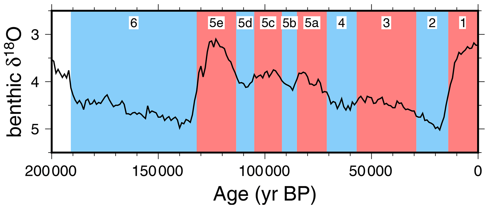
Figure 1 Definition of marine isotope stages. The black line is the LR04 benthic δ¹⁸O stack (Lisiecki and Raymo, 2005). The MIS stages denoted in red are warm interglacial and interstadial periods, while blue areas are colder glacial and stadial periods. The MIS 5 substage boundaries are from Otvos (2015), while the others are defined by Lisiecki and Raymo (2005).

Figure 2 MIS 5 sea-level indicators along the southeastern South America coastline (black-outlined circles).

Due to uncertainty in the age constraints, many of the features in this paper are assigned to MIS 5, rather than specifically to MIS 5e. However, due to the differences in sea-level height between the successive substages of MIS 5, in the absence of evidence for tectonic effects, specifically uplift, we infer that any sea-level record that has been attributed to MIS 5 corresponds to MIS 5e. This work is similar to other studies where there are multiple highstand records for MIS 5 present, in that MIS 5e features are expected to be those at the highest elevation (Lambeck and Chappell, 2001; Potter et al., 2004; Dumas et al., 2006; Surić et al., 2009; Moseley et al., 2013), MIS 5e features are expected to be those at the highest elevation. Many of the studies on shoreline deposits described in this database gave support for an MIS 5e substage assignment based on comparing the abundance of species of molluscs to infer paleo-water temperatures (e.g. Aguirre et al., 2006; Martínez et al., 2016). We have decided in our database to only include deposits that have numeric age control and are assigned an MIS 5 (or MIS 3; see Sect. 4.6) age by the original authors and to only use faunal evidence if used by the original authors. We acknowledge that due to the imprecision of the dating methods applied to the deposits in the entire study area, they may represent an MIS 5a or MIS 5c highstand or even Holocene or pre-MIS 5 highstands.

Patagonian Argentina was one of the first places in the world where multiple distinct indicators of past sea-level highstands were observed (Darwin, 1846). Due to the climatic conditions and minimal erosion, there is exceptional preservation of beach ridges and other relic Quaternary and Pliocene deposits along the entire coast, and they show remarkable continuity. North of Patagonia, in Buenos Aires Province, Pleistocene marine and estuary sediments have also been found (e.g. Aguirre and Whatley, 1995). For the WALIS database, we have only included sea-level indicators with sufficient depositional context to confidently assign an indicative range (aside from estuary deposits, which are here considered marine-limiting data points), sufficient elevation information to infer the paleo sea level, and chronological control that provides some confidence that the indicator is MIS 5 in age. The indicative range is the elevation range, relative to a fixed water level (i.e. mean sea level) in which a landform, deposit, or biological material will be found (Shennan, 2015).

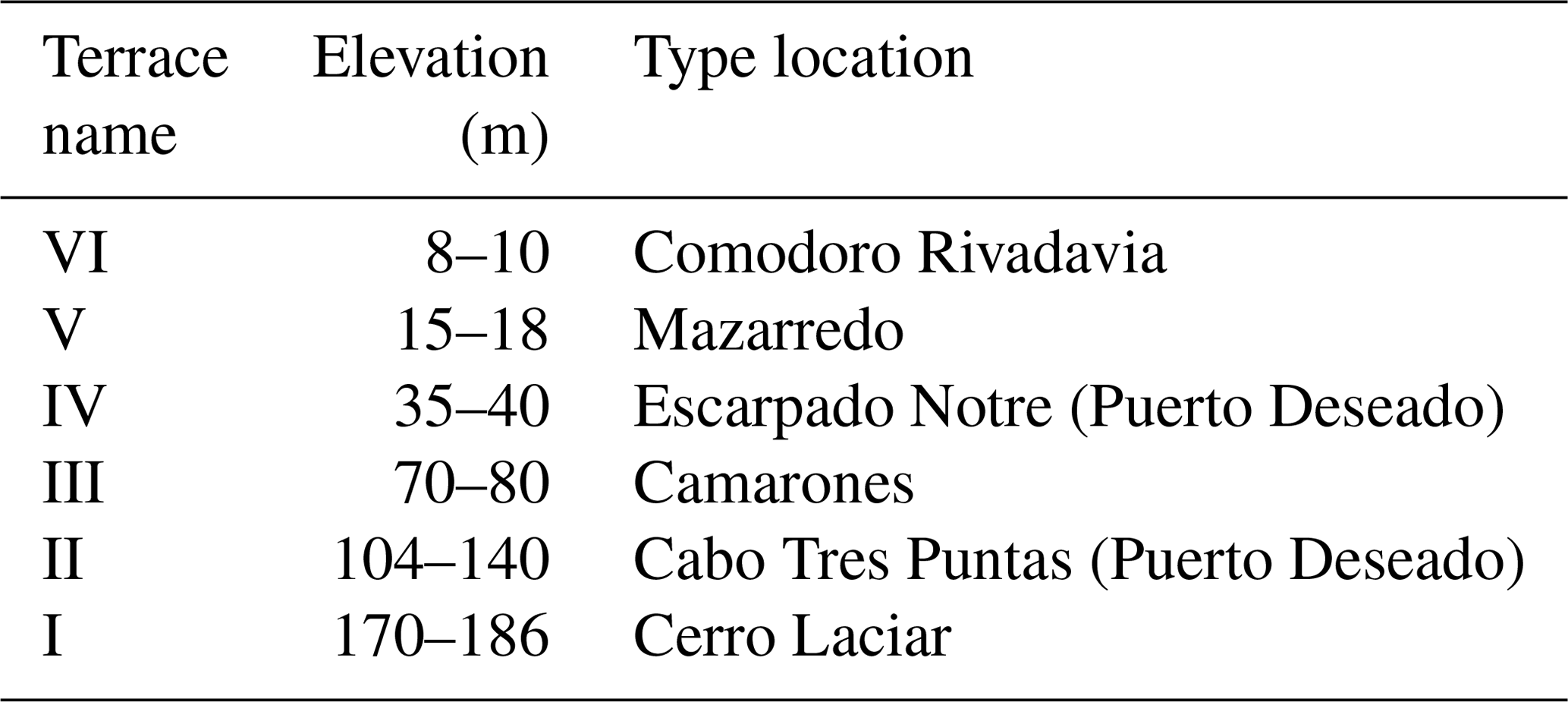
Geological indicators of multiple past sea-level highstands in Argentina (specifically Patagonia) were first measured and described in detail by Darwin (1846) in The Voyage of the Beagle. Darwin presented six cross sections of marine terraces, though only three of them had levels that are potentially last interglacial in age (most are reported at much higher elevations). Darwin remarked on how the elevation of different terraces seemed to be nearly the same along the entire Patagonian coast and concluded that their formation was likely the result of land being uplifted. This hypothesis continues to be favoured by many researchers working on Argentinian sea level (e.g. Pedoja et al., 2011; Isla and Angulo, 2016).

The commonly used nomenclature of Patagonian terrace levels was proposed by Feruglio (1950). In total, Feruglio (1950) identified and correlated six distinct terraces (I to VI, Table 1) on the basis of terrace elevation and fossil mollusc assemblage. Subsequent studies correlated Terrace V to MIS 5 (Codignotto et al., 1988; Rutter et al., 1989, 1990; Rostami et al., 2000). Feruglio's terrace nomenclature and correlations have continued to be used by subsequent authors. The next major set of studies on past Patagonian sea level was done by Codignotto and colleagues (Bayarsky and Codignotto, 1982; Codignotto, 1983, 1984, 1987), which was summarized by Codignotto et al. (1988). Many of these terraces were dated using radiocarbon measurements. Pre-Holocene terraces that returned finite dates were regarded by Codignotto et al. (1988) as belonging to the late Pleistocene.

Table 1 Terrace levels identified by Feruglio (1950).

From the late 1980s onwards, a number of studies presented chronological constraints allowing for a more confident MIS 5 assignment. Techniques used to date MIS 5 shorelines in Argentina include amino acid racemization (Rutter et al., 1989, 1990; Aguirre et al., 1995; Schellmann, 1998), electron spin resonance (Radtke, 1989; Rutter et al., 1990; Schellmann, 1998; Schellmann and Radtke, 2000), and U∕Th on mollusc shells (Radtke, 1989; Schellmann, 1998; Isla et al., 2000; Rostami et al., 2000; Bujalesky et al., 2001; Pappalardo et al., 2015). These studies provide the bulk of the confidently assigned MIS 5 sea-level proxies in the database.

The most recent review of past sea level in Argentinian Patagonia was by Pedoja et al. (2011). They split the coast into seven zones and measured elevations of changes in slope in the topography, which they interpreted as past sea-level highstands (shoreline angles). They reported up to nine slope angles in these zones. Their interpreted MIS 5 shoreline (named T1) indicates that there is spatial variability in the elevation.

2 Sea-level indicators

The descriptions of types of sea-level proxies found in Argentina are found in Table 2. The sea-level indicators include beach deposits (e.g. Fig. 3), beach ridges (e.g. Fig. 4), paleo-lagoonal deposits, and marine terraces. In addition, there are marine-limiting estuary deposits.

Pirazzoli (2005)2016Mauz et al. (2015)Rovere et al. (2016)Mauz et al. (2015)Rovere et al. (2016)Mauz et al. (2015)Rovere et al. (2016)Otvos (2000)Rovere et al. (2016)Otvos (2000)Rovere et al. (2016)(Rovere et al., 2016)(Zecchin et al., 2004)Rovere et al. (2016)Rovere et al. (2016)Zecchin et al. (2004)Perillo (1995)Perillo (1995)

Table 2 Different types of relative sea level (RSL) indicators reviewed in this study. RWL denotes reference water level, and IR denotes indicative range.

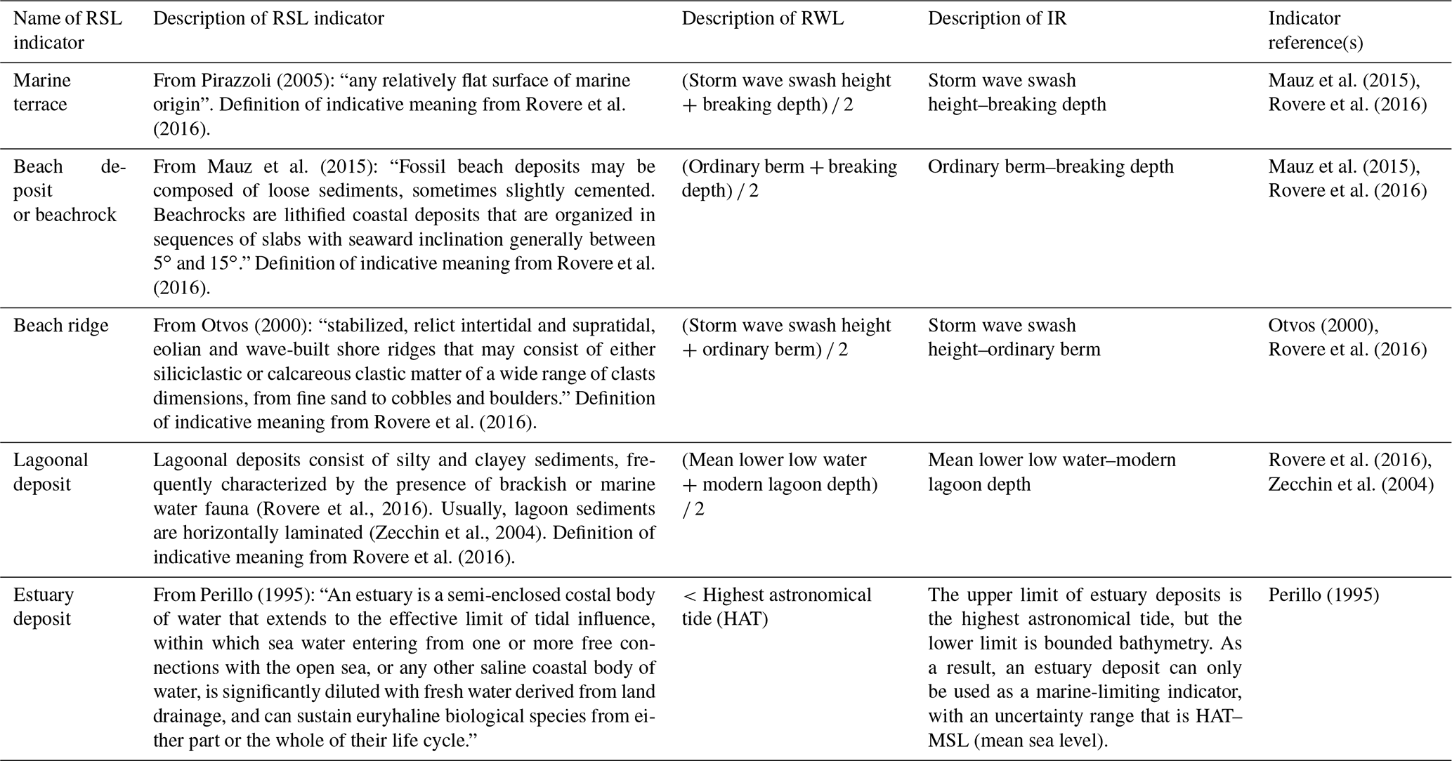
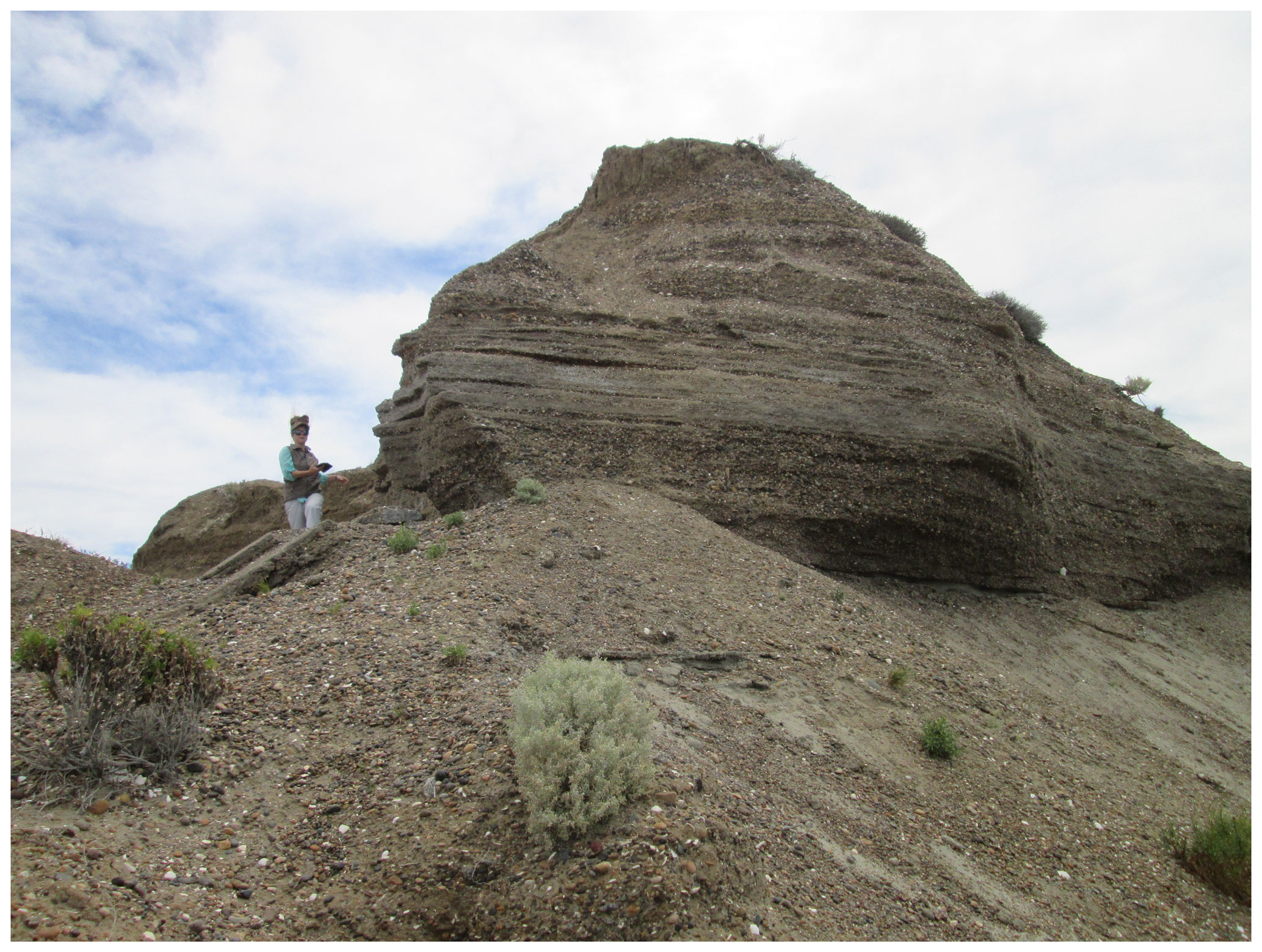
Figure 3 MIS 5 beach deposit near Caleta Olivia. The photo was taken on the front side of the beach deposit.

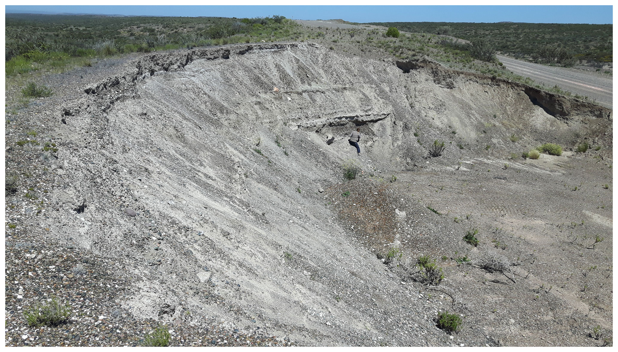
Figure 4 MIS 5 beach ridge deposit near Camarones. The photo illustrates the back side of the beach ridge, with the sea located on the left side of the photo.

For most of the data presented in this database, no indicative meaning or modern analogue was provided in the original studies. As a result, we use the IMCalc tool (Lorscheid and Rovere, 2019) to calculate the indicative range. IMCalc uses the definitions from Table 2 plus global wave and tidal models to estimate the indicative range at the location of the sample.

At multiple locations in northern Argentina, two Pleistocene or older estuary deposits are identified (Fig. 7). One is highly cemented and has not been analyzed by any numerical geochronological method. The second unit, overlying the highly cemented deposit, has returned finite radiocarbon dates. The interpretation of these radiocarbon dates is elaborated in Sect. 4. The estuary deposits are regarded as minimum-limiting indicators, as there is no limit to the depth at which they can be found (Perillo, 1995). The maximum limit is the highest astronomical tide, so it is necessary to apply the difference between the high tide level and median level to the elevation uncertainty.

In cases where elevations are reported as being relative to high tide, we provide a correction to make the reference to mean sea level. The tide statistics are taken from the Servicio de Hidrografía Naval website (http://www.hidro.gov.ar/oceanografia/Tmareas/Form_Tmareas.asp, last access: 20 January 2021). The tide tables only report the predicted astronomical component of the tide and do not take into account meteorological or steric components (Pappalardo et al., 2019). This will introduce an uncertainty of unknown magnitude to all data referenced to tidal datums from these sources (see Sect. 3).

Table 3 Summary of reviewed inferred MIS 5 sea-level data. For references refer to the text.

¹ SLI – sea-level indicator; ML – marine limiting; TL – terrestrial limiting. ² Quality ranges from 5 (excellent) to 0 (rejected). See Tables 3 and 4 for more information.

One of the challenges when making this database is that stratigraphic descriptions and interpretations of depositional environment are not stated. The beach ridge deposits of Patagonia are typically composed of gravel (Tamura, 2012), and deposition via wave action is certain. The beach ridges in Patagonia are typically interpreted as raised storm berms. The presence of marine shells within terrace beds allows for the inference that they are marine in origin. However, the lack of descriptions has prompted the assignment of low quality scores to some of these indicators. Studies with detailed stratigraphic context and, as a consequence, relatively high quality scores can be found in Schellmann (1998) and Rabassa et al. (2008). A summary of the indicators, along with quality assessment, is shown in Table 1.

3 Elevation measurements

Most of the reviewed studies report elevations measured by barometric altimeter or do not report an elevation measurement method (Table 5). Rostami et al. (2000) state that there is a strong suspicion that elevation in some studies may have just taken the value from Feruglio (1950) (which was likely derived from topography maps and Jacob's staff measurements), rather than from direct measurement. Pappalardo et al. (2019) did a further review of the vertical uncertainties of Argentinian sea-level indicators and stated that problems with misidentification of sea-level indicators and poor-quality elevation measurements hamper accurate assessments of paleo sea level. They also state that even within the same region, several studies disagree on what paleo sea level was during MIS 5, due to methodological differences in measuring elevation. The elevation measurements for previous studies were often made at the elevation of the shell samples used for dating, rather than made measuring the thickness of the geological unit that would provide a more robust estimate of the true paleo-sea-level range. As an example (Table 1 in Pappalardo et al., 2019), at Camarones, estimates of MIS 5 sea level ranged between 7.5 and 17 m in different studies.

Due to the ambiguity of elevation measurements, a high degree of uncertainty is assigned to many sea-level indicators. An additional 20 % uncertainty (a value recommended by Rovere et al., 2016) was added to altimetric measurements since this method is less reliable than levelling or differential GPS and results can vary depending on atmospheric conditions. This added uncertainty is further justified as most altimetric measurements lack details on how they were referenced to sea level. An additional source of uncertainty is when a section is described, but it is not clear if the reported elevation refers to the top or the bottom of the section. In these instances, the entire thickness of the section is added to the error. When the details of where on the outcrop or landform the elevation was measured are not stated, the elevation error is assigned to be 20 % of the reported elevation from the highest reported elevation. Either all elevations were reported in reference to mean sea level (often referenced to a local tide gauge), or, for studies in which no sea-level datum is defined, the measurements were assumed to be referenced to mean sea level for entry into WALIS. This definition may have complications as the local “mean” sea level can have an offset from the global mean sea level (or orthometric elevation) (Lanfredi et al., 1998; Pappalardo et al., 2019), which has not been accounted for in our entries. Sites that were reported from a high-tide datum have been corrected to mean sea level using the values from nearby tidal charts (see Sect. 2).

Table 4 Quality scores for RSL, from the WALIS documentation.

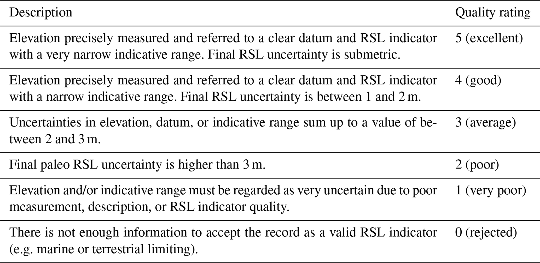
In some locations, it is possible that the same outcrop is described by multiple studies. However, since the precise locations of these deposits are not always clear, each record is included as a separate indicator, with individual elevation uncertainties. Indicators for which it was not possible to determine an exact location are included in the database, since they may have some utility in future modelling studies, but are given the lowest quality score (zero). An overview of the quality score criteria for RSL is in Table 3.

4 Dating techniques

MIS 5 deposits in southeastern South America have been dated using amino acid racemization (AAR) values, electron spin resonance (ESR), uranium–thorium dating (U∕Th), optically stimulated luminescence (OSL), infrared stimulated luminescence (IRSL), and radiocarbon methods. Marine shell fossils (Fig. 5), often still articulated, are abundant in many shoreline deposits. AAR, ESR, and U∕Th techniques can provide a confident MIS 5 age assignment provided there has been limited chemical alteration. These methods can be used to distinguish shells of MIS 5 from earlier interglacials or the Holocene but lack the resolution to differentiate between substages of MIS 5, i.e. 5e, 5c, or 5a. A wide variety of bivalve and gastropod species have been used for dating, which are listed in Table 6. Radiocarbon and, to some extent, OSL dates have been used to establish minimum ages, proving that a deposit is older than the Holocene. Other absolute dating techniques, the environmental context from fauna, and stratigraphic position can be used to support an MIS 5 age assignment. An overview of the quality score criteria for age constraints is in Table 4. In this compilation, for any site where minimum ages are the only chronological control, we give a low quality assignment (i.e. zero out of five). We did not include features that have no dating applied to them in WALIS, though for some locations we have noted them in the text.

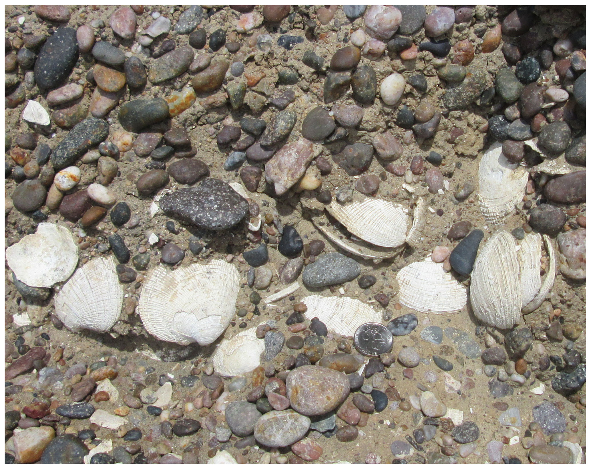
Figure 5 Well-preserved MIS 5-aged fossil shells from a deposit near Caleta Olivia. The coin is 23 mm in diameter.

Table 5 Quality scores for age, from the WALIS documentation.

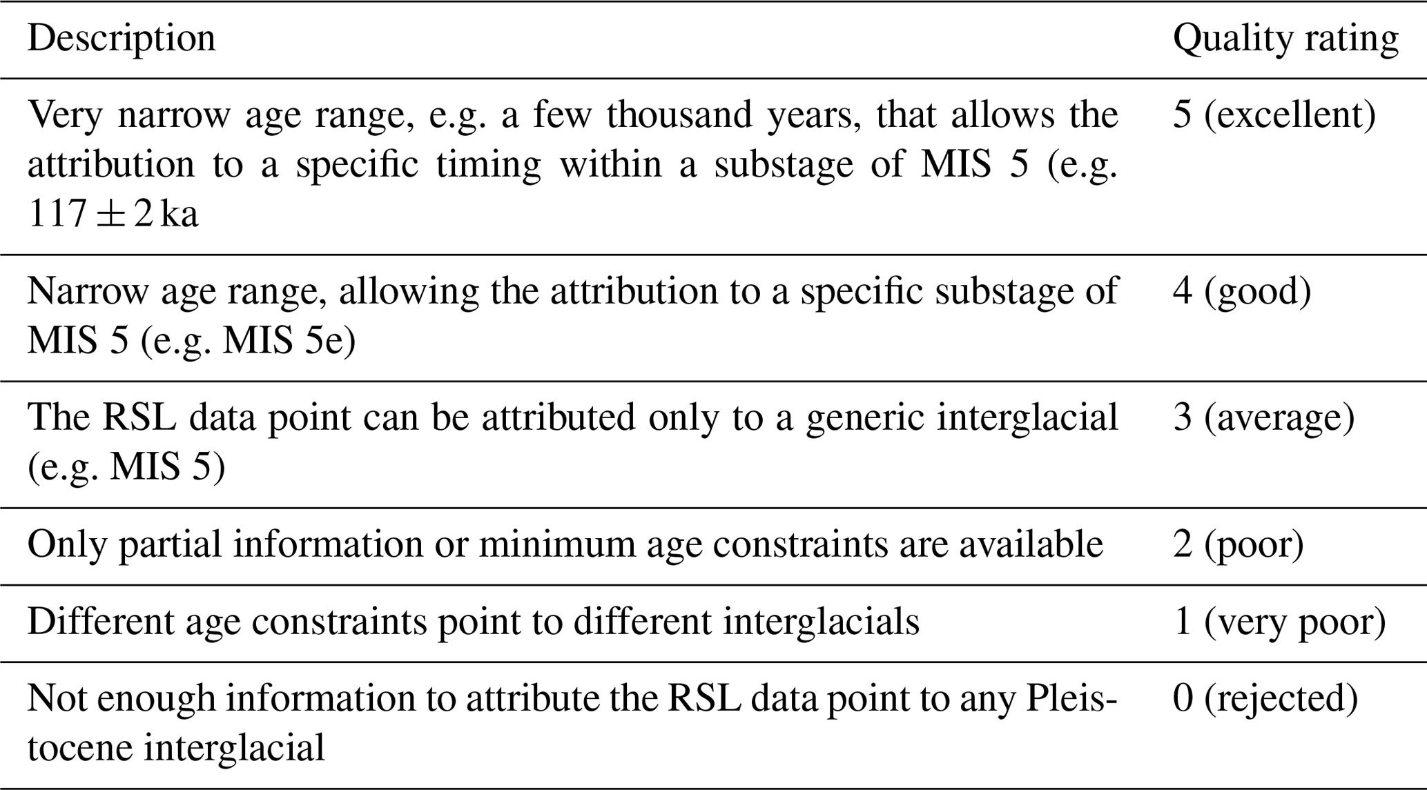
Table 6 Measurement techniques used to establish the elevation of MIS 5 shorelines in Argentina.

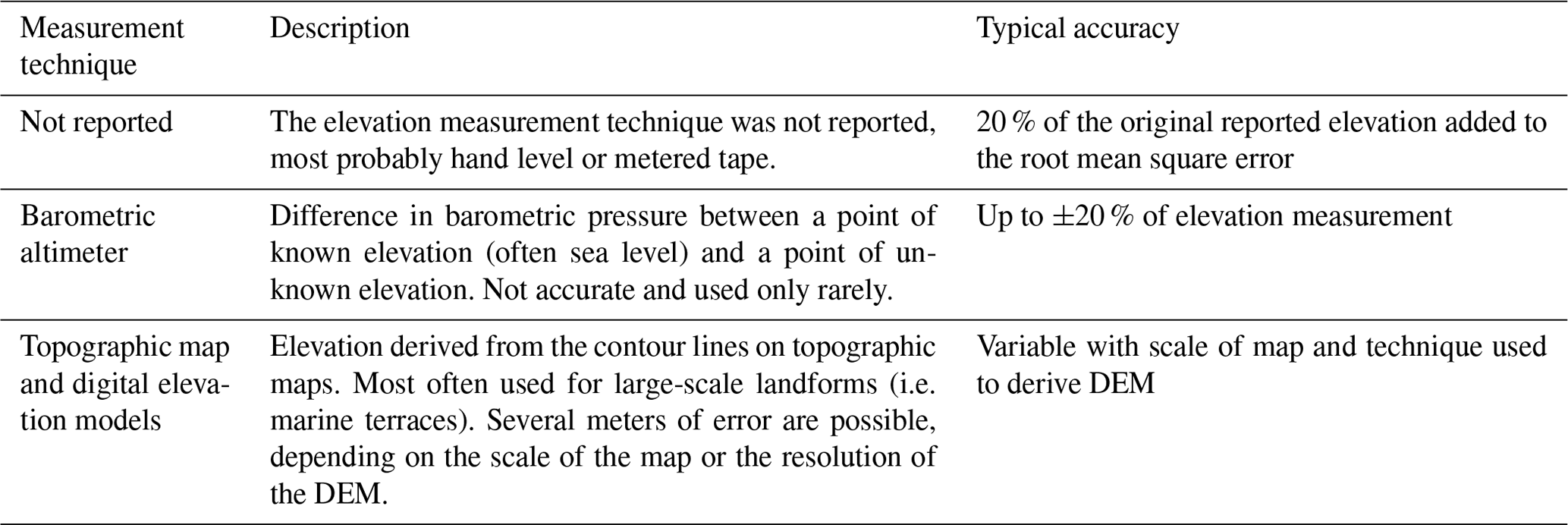
Table 7 Species of shells that have been dated in southeastern South America. Names are as reported in the original papers.

¹ Standard spelling Brachidontes rodriguezii. ² Full species name unknown. ³ Standard spelling Perumytilus purpuratus. ⁴ Full species name Protothaca antiqua.

4.1 Amino acid racemization (AAR)

The analytical procedure for AAR is reported by Rutter et al. (1989). They reported aspartic acid and leucine values of multiple species of shells, without analytical uncertainties. They did not report numerical ages, only using the values to distinguish between deposits of different ages. Aguirre et al. (1995) reported numerical ages from AAR, calibrated with Holocene shells of the same species. However, due to the non-linear kinematics of racemization, this approach is not recommended in Pleistocene shells (Clarke and Murray-Wallace, 2006). In order to draw correlations, the same species should be used, since the racemization is species dependent. This is not possible in many of the locations where AAR samples have been reported in our study area.

4.2 Electron spin resonance (ESR)

The details of ESR dating can be found in Rutter et al. (1990) and Schellmann and Radtke (1997, 1999). The main issue with ESR is that mollusc shells are not a closed system to uranium, so therefore it cannot be assumed that the uranium concentration has been constant since deposition (Radtke et al., 1985; Schellmann and Radtke, 1999). As a result, Schellmann and Radtke (1997) recommended using the “early-uptake” model for determining the age. Under this hypothesis, most of the uranium was taken up in the shell within the first 10 000 years of deposition. Although this approach will give younger ages than the commonly used “linear-uptake” model, Schellmann and Radtke (1997) regarded it as being more accurate. All of the ages in this database use the early-uptake model. The early ESR dates (Radtke, 1989; Rutter et al., 1990) are not reported with an uncertainty, so we use a value of 15 % of the age, as recommended in those studies. Schellmann and Radtke (1999) tested their methods on a number of articulated shells from a deposit in Camarones and showed a large spread in ages (dating to between 92–171 ka), which demonstrated the care that must be taken in interpreting the results of ESR dating. Due to the uncertainty in the uranium uptake history of shells, it is not possible to use this method to distinguish between substages in MIS 5, even if the reported ages indicate ages that are younger than MIS 5e.

4.3 U∕Th dating

The U∕Th dating done by Radtke (1989) was accomplished using mass spectrometry. The measurements were done at three laboratories; University of Cologne, Heidelberg University, and McMaster University. The University of Cologne laboratory corrected for excess thorium using the formula $-\left({}^{\mathrm{232}}\mathrm{Th}\times (\mathrm{3}\mathrm{ppm}\mathrm{U}/\mathrm{12}\mathrm{ppm}\mathrm{Th})\times \mathrm{0.378}\right)$ if the thorium was in excess of 0.3 ppm. This corrected value was preferred by Radtke (1989). Rostami et al. (2000) reported U∕Th analysis on shells using alpha spectrometry. The ages were generally consistent with ESR dates from the same deposits. Pappalardo et al. (2015) also used this method for dating shells, using mass spectrometry, and also returned dates consistent with ESR dating. As with ESR dating, the reliability of U∕Th ages of mollusc shells are questionable since they are not closed systems for uranium (Radtke et al., 1985). When Radtke et al. (1985) compared ESR and U∕Th ages of the same shells, they found that the similarity between the two methods was species dependent, and for some the measured ages could be very different from independently derived ages of deposits. Deriving accurate ages from mollusc shells using this method requires careful analysis of the uranium uptake history of the shell (i.e. using the ICPMS method), and precise and accurate dates may not be possible without it (Eggins et al., 2005). As a result, shells dated using the U∕Th method in the study area can only provide a general assignment to MIS 5 and are not precise enough to determine a specific substage.

4.4 Optically stimulated luminescence (OSL)

OSL ages were derived from quartz grains of samples collected at two sites in Uruguay (Rojas and Martínez, 2016) and three sites in Argentina (Martínez et al., 2016; Zárate et al., 2009; Beilinson et al., 2019). Analysis for the Uruguay samples and the site at Ezeiza, Argentina, was completed at the University of Illinois at Chicago (Rojas and Martínez, 2016; Martínez et al., 2016). The samples were collected using a PVC pipe with only the inner part of the sample retained for analysis. The OSL sample at Nicolás Vignogna III Quarry was analyzed at Dataçao Labs (Beilinson et al., 2019). The samples were collected using metal tubes and opaque black bags. The samples from Hudson, Argentina, were collected from blocks of sediment extracted from the outcrop (Zárate et al., 2009).

4.5 Infrared stimulated luminescence (IRSL)

IRSL ages from K-feldspar grains were collected from the Puerto Williams site in Chile (Björck et al., 2021). K-feldspar was chosen over quartz as the luminescence signal was too weak in the quartz. The date derived from the pIRIR signal at 290 ^∘C, with the assumption of no fading, was chosen to represent the age. Analysis was completed at Lund University.

4.6 Radiocarbon

During the 1980s and 1990s, a lot of debate centered on the age of the Pleistocene shorelines, as conventional radiocarbon dating provided finite dates. González et al. (1988b) detailed the method of radiocarbon dating as applied to Pleistocene deposits. Despite careful pretreatment of the shells from deposits suspected to be MIS 5 in age, the conventional radiocarbon method returned finite ages for pre-Holocene shells. The result of these finite dates led some authors to suggest the possibility of an MIS 3 sea-level highstand record along the Argentinian coast (Codignotto et al., 1988; González et al., 1988b; González, 1992; Aguirre and Whatley, 1995). González and Guida (1990) supported this interpretation through the use of magnetostratigraphy and correlating reverse magnetized stratigraphic units to magnetic excursions (see Sect. 4.7). Cionchi (1987) and Radtke (1988) rejected the interpretation of the finite ages as reliable and suggested that they were contaminated with secondary carbonates. With the introduction of other dating techniques applied to Argentinian coastal deposits, the assignment of an MIS 3 age became untenable (Rutter et al., 1989, 1990, 1992; Aguirre et al., 1995). Rojas and Martínez (2016) concluded that MIS 3-aged shells found in Uruguay Pleistocene deposits were minimum ages, since the shell species were consistent with warmer-than-present water temperatures, something that was unlikely to be true during the MIS 3 period. Radiocarbon dating remains the most widely applied method to date Holocene shorelines and has been successfully applied to many of the same regions that have Pleistocene deposits (see Sect. 6.4).

Radiocarbon dating of suspected Late Pleistocene material like shells requires careful pretreatment to remove secondary precipitates and other contaminants (Wood, 2015). Techniques to produce reliable dates are reliant on accelerator mass spectrometry (AMS) radiocarbon measurements, so the conventional radiocarbon ages previously acquired in South American deposits should be regarded, in the absence of further constraints, as minimum ages. However, we suggest that minimum ages can still be used to distinguish between Holocene and Pleistocene deposits, the latter characterized by minimum radiocarbon ages. This is confirmed by the fact that, in some places, Pleistocene deposits have been dated by both radiocarbon and other techniques (Rutter et al., 1989, 1990; Aguirre et al., 1995; Rojas and Martínez, 2016). Marine deposits with minimum radiocarbon ages and at an adjacent elevation above the Holocene highstand position have been assigned to MIS 5 within WALIS. These data should be treated with caution and regarded as being of extremely poor quality.

4.7 Paleomagnetism

González and Guida (1990) reported paleomagnetic measurements as a way to distinguish between differently aged Pleistocene shoreline deposits. In their paper, they reported reverse magnetized sediments, which they assigned MIS 3 and MIS 5 ages on the basis of correlation to magnetic excursions (i.e. geologically brief periods of a weak or reversed magnetic field). They regarded definitively reversed sediments to be correlative to the Blake Excursion. The Blake Excursion happened during MIS 5d, between 112–116 ka (Rossi et al., 2014). Since the MIS 5 highstand more likely happened during MIS 5e and MIS 5d sea level was tens of meters below the present sea level (Lambeck and Chappell, 2001), either the magnetic measurements are in error or the deposit is not MIS 5e in age. González and Guida (1990) interpreted some deposits with anomalous magnetism that also had finite radiocarbon ages as being correlative to the Lake Mungo excursion. The Lake Mungo excursion was reported to have happened at about 30 ka, but recently this has been discredited (Roberts, 2008). We put no confidence in the ability of these measurements to assign an age to the deposits and do not use them to assign an MIS 5 age.

4.8 Stratigraphy

South American geologists who have worked on paleo sea level have tended to use the glacial–interglacial chronostratigraphic nomenclature used in North America. The Wisconsin glaciation represents the most recent glacial period, covering MIS 5d-2 (Otvos, 2015). The Sangamon interglacial represents the last interglacial, broadly defined as the period when there were dominantly non-glacial conditions in the Americas. Some definitions place the Sangamonian to encompass all of MIS 5, but more recent definitions narrow it to only MIS 5e (Otvos, 2015). It is therefore roughly equivalent to the European Eemian Stage, which strictly correlates with MIS 5e (Mangerud et al., 1979). In Buenos Aires Province, the marine transgression correlated to MIS 5 is called the Belgranense Stage (Aguirre and Whatley, 1995; Isla et al., 2000; Martínez et al., 2016; Rojas and Martínez, 2016). At only one location identified in this review, Isla Navarino, Chile, is the age of the sea-level indicator constrained on the basis of its stratigraphic position below Wisconsin-aged glacial sediments.

5 Relative sea-level indicators

In total, we reviewed 60 documented possible MIS 5 sea-level proxies, of which 48 are sea-level indicators, 11 are marine-limiting points, and 1 is terrestrial limiting. A plot of the elevation of these proxies is presented in Fig. 10. Sea-level indicators have enough information to tie the feature to sea level, while marine-limiting and terrestrial-limiting points only have enough information to place the feature below or above sea level, respectively. The paleo sea level is calculated using the indicative range of the indicator, the reported elevation and thickness of the indicator, and the uncertainties applied to those measurements. The elevation of sea-level indicators along the coast ranges between 0 and 30 m above mean sea level (a.m.s.l.). This large range reflects the uncertainty in elevation measurements; however, it could also reflect incorrect correlation to MIS 5e. There is also the possibility that the elevation variability is a real feature related to glacial isostatic processes (see Sect. 6.5.2). The locations in this section are described in order of north to south along the southeastern South American coast.

5.1 Uruguay

Uruguay has data at three locations (Fig. 6).

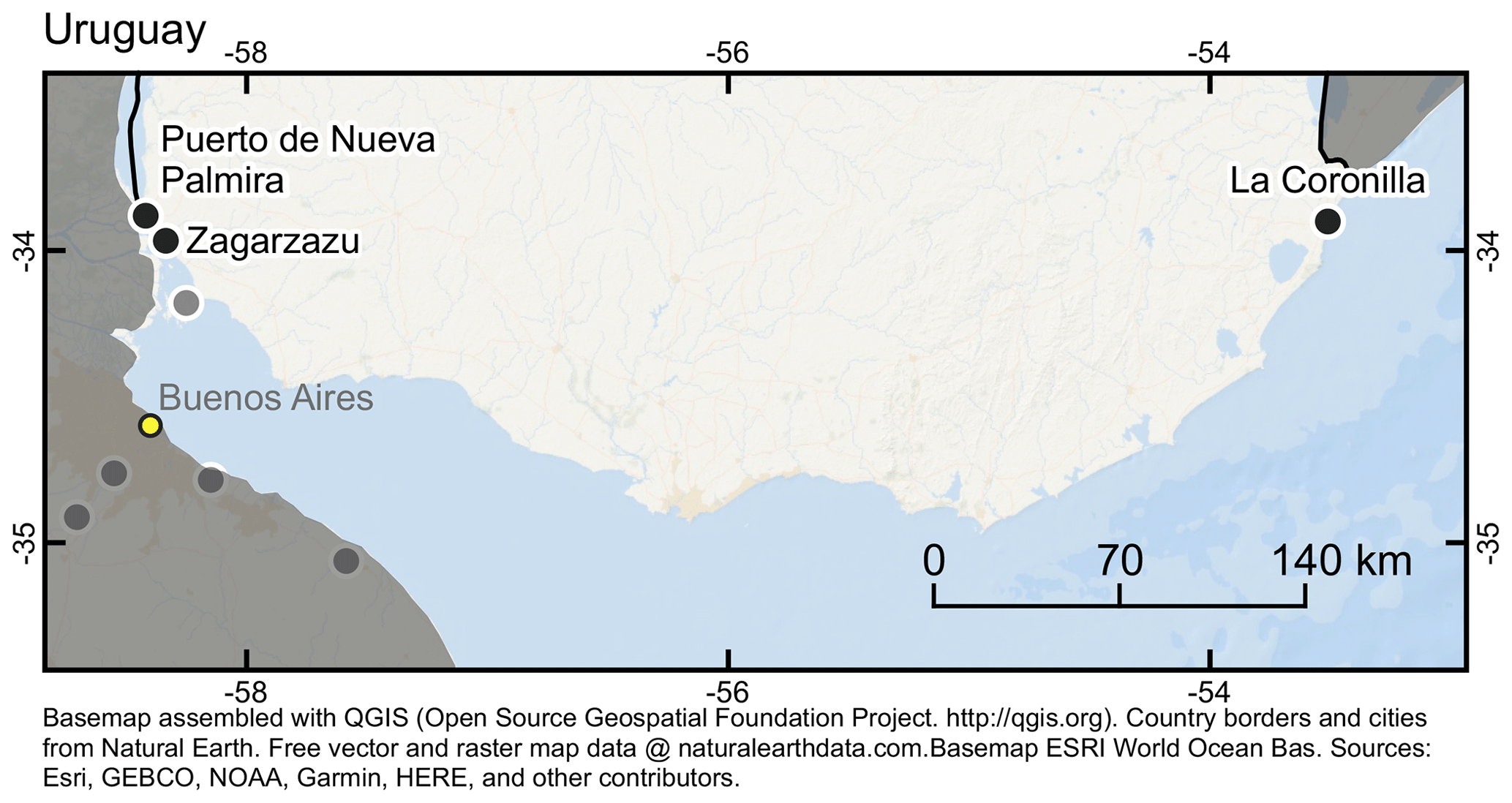
Figure 6 MIS 5 sea-level indicators in Uruguay (black circles).

5.1.1 La Coronilla

Martínez et al. (2001), Rojas and Martínez (2016), and Rojas et al. (2018a) describe a 0.6 m thick marine deposit with abundant marine mollusc fossils located at the modern coast. They interpreted the deposit to represent a low-energy environment, such as a bay. The age of the deposit is only constrained with minimum-age radiocarbon dates. A taxonomic analysis by Rojas et al. (2018b) identified many species that are currently found 600 km north of La Coronilla, indicating warmer-than-present water conditions, which they interpreted as supporting an MIS 5e age assignment. The marine-limiting elevation is 0.50 ± 0.53 m.

5.1.2 Zagarzazú

Rojas and Martínez (2016) and Rojas et al. (2018a) described a thin (0.5 m) exposure of marine sediments at the modern coast containing shells in living position. A radiocarbon date from this site yielded a minimum-limiting date, while an OSL date supports an MIS 5a age assignment. The marine-limiting elevation is 0.50 ± 0.53 m. An analysis of the fossil shell species indicated that conditions were more saline than at present, but since there were fewer warm-water species than in the La Coronilla section, they concluded an MIS 5a age was more likely (Rojas and Martínez, 2016).

5.1.3 Puerto de Nueva Palmira

Marine deposits, interpreted as having been deposited in a proximal, wave-dominated environment, at Puerto de Nueva Palmira were described by Martínez et al. (2001), Rojas and Martínez (2016), and Rojas et al. (2018a). The deposit (about 1.5 m thick) contained disarticulated, randomly oriented shell fossils. Martínez et al. (2001) collected two minimum-age radiocarbon dates from this deposit but interpreted the deposit as being from the last interglacial on the basis of marine fauna indicating a relatively warm environment. Rojas and Martínez (2016) reported an OSL date of 80.7 ± 5.5 ka, which suggests an MIS 5a assignment, but they were cautious about assigning a specific substage of MIS 5 to the deposit. From faunal analysis, they suggested that the environment was not necessarily warmer, as the La Coronilla assemblage suggests. This means an MIS 5a assignment is plausible. This deposit gives a marine-limiting elevation of 12.5 ± 2.8 m.

5.2 Northern Argentina – Entre Ríos and Buenos Aires provinces

Entre Ríos Province and Buenos Aires Province have data at 14 locations (Fig. 7).

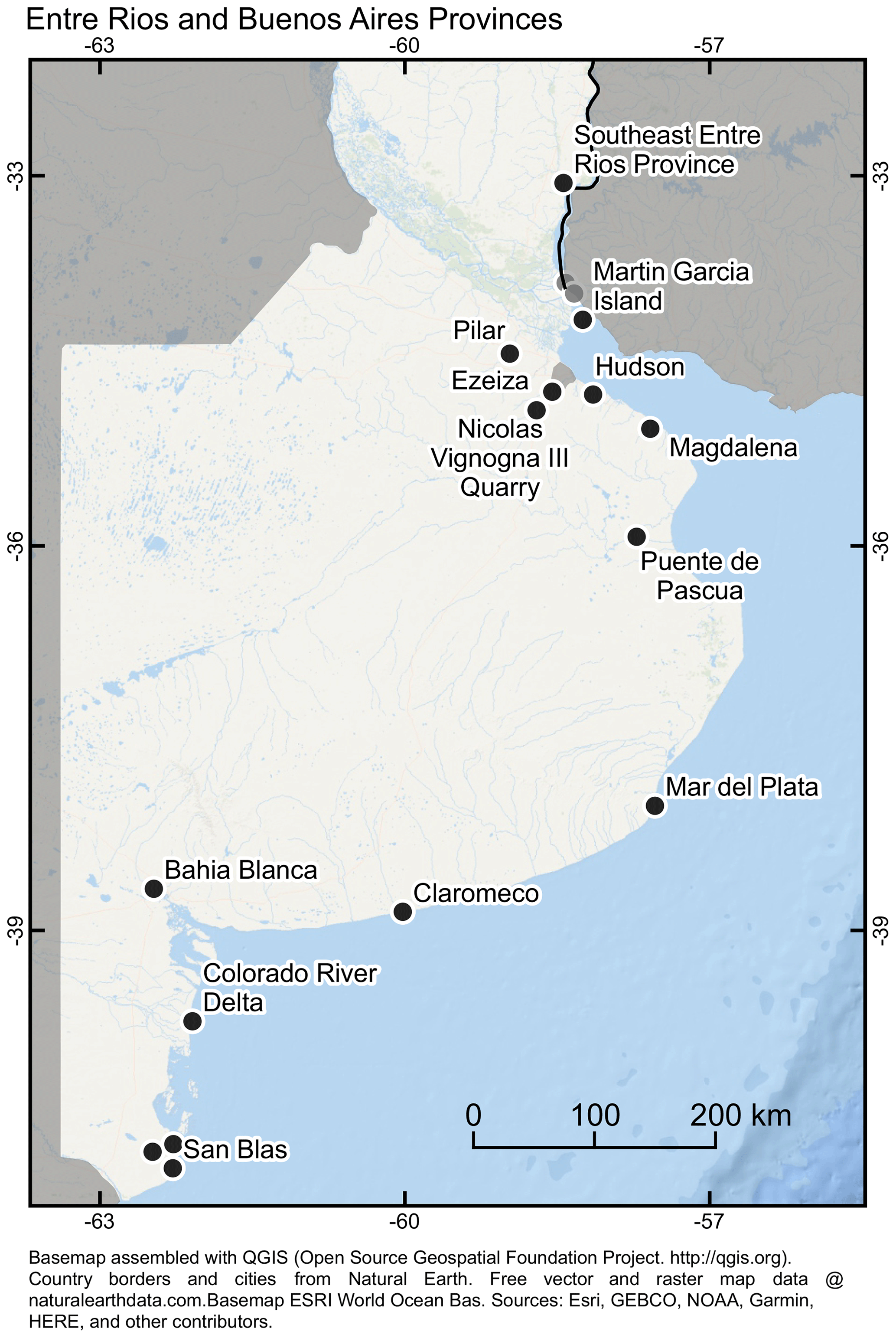
Figure 7 MIS 5 sea-level indicators in Entre Ríos and Buenos Aires provinces, Argentina (black circles).

5.2.1 Southeast Entre Ríos Province

González et al. (1986, 1988b) and González and Guida (1990) describe a Pleistocene estuary deposit in a location called Irazusta Quarry. The exact location is estimated based on a map from the paper but is likely over 100 km from the modern coast. The deposit was about 1.2 m thick and contained shells that indicate a brackish environment, overlying a relic shore platform. They collected three finite radiocarbon dates, but these are regarded as minimum ages. The minimum sea level from this deposit is 6.2 ± 1.5 m. We applied an uncertainty from the modern tidal range using the nearest tide gauge, on Martín García Island. Based on the similarity in elevation of this deposit to the Magdalena site (see Sect. 5.2.7), we infer it is MIS 5 in age.

González et al. (1988b) and González and Guida (1990) completed magnetostratigraphic analysis of the substrate upon which the platform surface was formed, a lagoon deposit. The reverse polarity of the sediments prompted correlation of the lagoon deposit with the Blake Excursion, a minor reversal during MIS 5d. However, due to the implications for the necessary uplift to place MIS 5d sediments above modern sea level (see Sect. 4.7), this correlation is considered to be incorrect.

5.2.2 Martín García Island

González and Ravizza (1987) and González et al. (1986) describe a thin (0.4 m) Pleistocene estuary deposit adjacent to a paleo-cliff on Martín García Island. Based on finite radiocarbon ages, they assigned an MIS 3 age; we regard this as an minimum age. Based on similar elevation and stratigraphy to the Magdalena site (Sect. 5.2.7), we regard this deposit to be MIS 5 in age. The marine-limiting elevation from this deposit is 7.5 ± 1.7 m.

5.2.3 Pilar

Fucks et al. (2005) describe a Pleistocene-aged estuary deposit, with a maximum elevation of 8 m. A radiocarbon-dated shell returned an infinite age. If this deposit is MIS 5 in age, it has a marine-limiting elevation of 8 ± 1.8 m. Based on the similarity in elevation to the Magdalena site (Sect. 5.2.7), we regard this as an MIS 5 deposit.

5.2.4 Ezeiza

Martínez et al. (2016) investigated mollusc fauna from marine sediments exposed at a riverbank in Ezeiza. Two radiocarbon dates from the deposit gave minimum-limiting dates. The species found in the sediment indicate warmer-than-present water conditions, which led them to conclude the sediment corresponds to MIS 5e. The marine-limiting elevation is 3.5 ± 0.8 m.

5.2.5 Nicolás Vignogna III Quarry

Beilinson et al. (2019) described a sedimentary sequence in a quarry southwest of Buenos Aires (Fig. 7). There were three facies they interpreted as being associated with MIS 5. The lowest facies was interpreted as a salt marsh; the second facies was deposited in a coastal creek environment, and the upper facies is composed of beach-like deposits associated with storm surges. In the present day, storm surges that form these kind of deposits reach between 1 and 4.4 m above present sea level. The environmental conditions derived from fossils in the deposit indicate a range of conditions, from freshwater to marine, so we interpret this as being terrestrial limiting (i.e. forming above mean sea level but influenced by seawater at least periodically). Gasparini et al. (2016) reported a radiocarbon date from the beach-like deposit and, due to the sedimentary environment, considered it to be terrestrial limiting. An OSL date from the beach-like deposit gave a date of 60 ka (Beilinson et al., 2019), which also likely underestimates the true age. If this deposit formed during MIS 5, it gives a terrestrial-limiting elevation of 1.3 ± 3.1 m.

5.2.6 Hudson

Zárate et al. (2009) described a section located at Hudson (Fig. 7). Within the section was a laterally discontinuous marine clayey silt, interpreted as being deposited in a distal tidal channel, with marine fossils. OSL dating of this unit is consistent with an MIS 5 age assignment. The marine-limiting elevation is 6.1 ± 1.9 m.

5.2.7 Magdalena

Weiler et al. (1988) and González et al. (1986) describe a thin (0.2 m) estuary deposit beneath a paleo-cliff deposit at Cañada de Arregui, near Magdalena. Radiocarbon ages from this deposit gave minimum ages (Aguirre et al., 1995). Aguirre and Whatley (1995) and Aguirre et al. (1995) collected Tagelus sp. mollusc shells for AAR analysis from the same outcrop. The AAR values for the outcrop were higher than Holocene samples from the same location. Using the Holocene data for calibration, a numerical age dating to 106 ka was determined, which is consistent with an MIS 5 age. The minimum sea level from this deposit is 6.0 ± 1.7 m. Although this site has relatively good age control, the lack of information on elevation measurements means that it is relatively low quality.

5.2.8 Puente de Pascua

Aguirre and Whatley (1995) and Aguirre et al. (1995) collected Tagelus mollusc shell samples for AAR dating from a well-cemented coquina at Puente de Pascua. An AAR date of 123 ka is consistent with an MIS 5 deposit. However, insufficient information is given to ascertain an indicative meaning, so we assign this data point as marine limiting, with an elevation of 3.5 ± 1.3 m.

Fucks et al. (2006, 2010) returned to this location and undertook a further investigation of the MIS 5 deposit. They reported a 0.7 m thick sand deposit with lenses of shells that they interpreted to be a beach deposit. The reported elevation of the deposit (6–8 m) is higher than that reported by Aguirre and Whatley (1995) and Aguirre et al. (1995) (3–4 m). The calculated sea level from this deposit is 6.8 ± 4.0 m.

5.2.9 Mar del Plata

González et al. (1986) gave a brief description of a transgressive beach deposit. Radiocarbon dating provided minimum ages. A magnetostratigraphic analysis of this deposit showed that it has negative magnetic polarity. González and Guida (1990) interpreted this to be correlative to the Lake Mungo magnetic excursion, which they correlated to MIS 3 on the basis of the radiocarbon dates (which they regarded as reliable). We have included this point as an MIS 5 deposit based on elevation. Though if the magnetic measurements are reliable, this would indicate that an MIS 5e age assignment is unlikely. The calculated sea level from this deposit is 10.3 ± 2.5 m.

5.2.10 Claromecó

Isla et al. (2000) and Isla and Angulo (2016) reported on a beach deposit that was assigned to MIS 5 using a U∕Th date. The calculated sea level from this deposit is 7.0 ± 2.0 m.

5.2.11 Bahía Blanca

González et al. (1986, 1988b) described an estuary deposit, overlying a cemented delta deposit. The estuary deposit contained many mollusc fossils that had minimum radiocarbon ages. The minimum sea level from this deposit is 13.5 ± 3.6 m. The relatively high elevation of this deposit and the Holocene highstand deposits (> 10 m a.m.s.l.) led González et al. (1988b) to hypothesize that this location is uplifting. Aliotta et al. (2001) investigated these deposits and concluded that the depositional environment during the Pleistocene was lower energy than that during the Holocene highstand.

5.2.12 Colorado River delta

González et al. (1986, 1988b) briefly described a beach ridge deposit with fossil mollusc shells that had minimum radiocarbon ages. The calculated sea level from this deposit is 4.8 ± 1.8 m. Fucks et al. (2012a) also mapped Pleistocene marine deposits that they correlated to MIS 5 in the Colorado River region, but there is not enough information for an assessment of paleo sea level. Charó et al. (2015) investigated the faunal composition at sites they interpreted to be MIS 5e and found the faunal content was similar to that of Holocene deposits. Since they did not present any numerical dating, there is not enough information to include these sites in the database.

5.2.13 Bahía Anegada

Weiler (1993) described several individual pre-Holocene beach ridge deposits in Bahía Anegada. These deposits had minimum radiocarbon ages. Unfortunately, elevation measurements are not available, and this location was not added to the database.

Fucks et al. (2012a) revisited the sites and reported elevations of 8–10 m, which was possibly based off values from topographic maps or Google Earth. They correlated them to MIS 5 on the basis of similar elevation to other dated landforms in the region. However, there is not a sufficient description of the deposits or of dating to include them in our database. Charó et al. (2013a) further analyzed the faunal content and found a higher abundance of species in the deposits attributed to MIS 5e, which they interpreted to indicate warmer water conditions.

5.2.14 San Blas

Trebino (1987) described the geomorphology and raised shorelines in the San Blas area. They described two groups of shorelines: one that was Holocene in age and another that was determined to be Pleistocene on the basis of finite radiocarbon dates. The Pleistocene group, at a higher elevation, consists of three beach ridges with elevations of 9–10 m. We correlate the shorelines to MIS 5, with low confidence. Trebino (1987) reported that the modern elevation range for coastal dune and beach deposits is between 0.5 and 7 m, which we take as the modern analogue. We calculate a paleo sea level of 5.8 ± 3.8 m from these shorelines.

Rutter et al. (1989) collected fossil mollusc shells at two sites in San Blas, both of which were interpreted as being Pleistocene in age on the basis of AAR values. The samples were taken from a 1.2 m thick beach deposit (SB-2) and a 6 m thick beach gravel layer within a 10 m high section (SB-1). When comparing the same species, the AAR values were generally lower for the samples taken at SB-2 than for those taken at SB-1, which implies the SB-1 site represents an older deposit. Rutter et al. (1989) defined the SB-2 deposit as an “intermediate”-aged deposit, older than Holocene, and cautiously assigned an MIS 5 age. The calculated sea level of SB-2 is 12.4 ± 3.1 m. ESR dating of mollusc shells from the deposit at SB-1 returned ages that were consistent with an MIS 5 age (Rutter et al., 1990), which contradicts the authors' earlier interpretation that the deposit is significantly older. If accepted as being MIS 5, the calculated sea level is 4.0 ± 3.9 m. Fucks et al. (2012a) also investigated this location and reported on mollusc species. Charó et al. (2013b) compared the faunal content of shoreline deposits attributed to MIS 5e and the Holocene in the San Blas area. Due to the presence of Crassostrea rhizophorae, they interpreted the conditions to be warmer in the MIS 5e deposits, although overall, the species content was similar. Since these deposits do not have numerical ages, we do not include them in the database.

5.3 Patagonia – Río Negro Province

Río Negro Province has data at one location (Fig. 8).

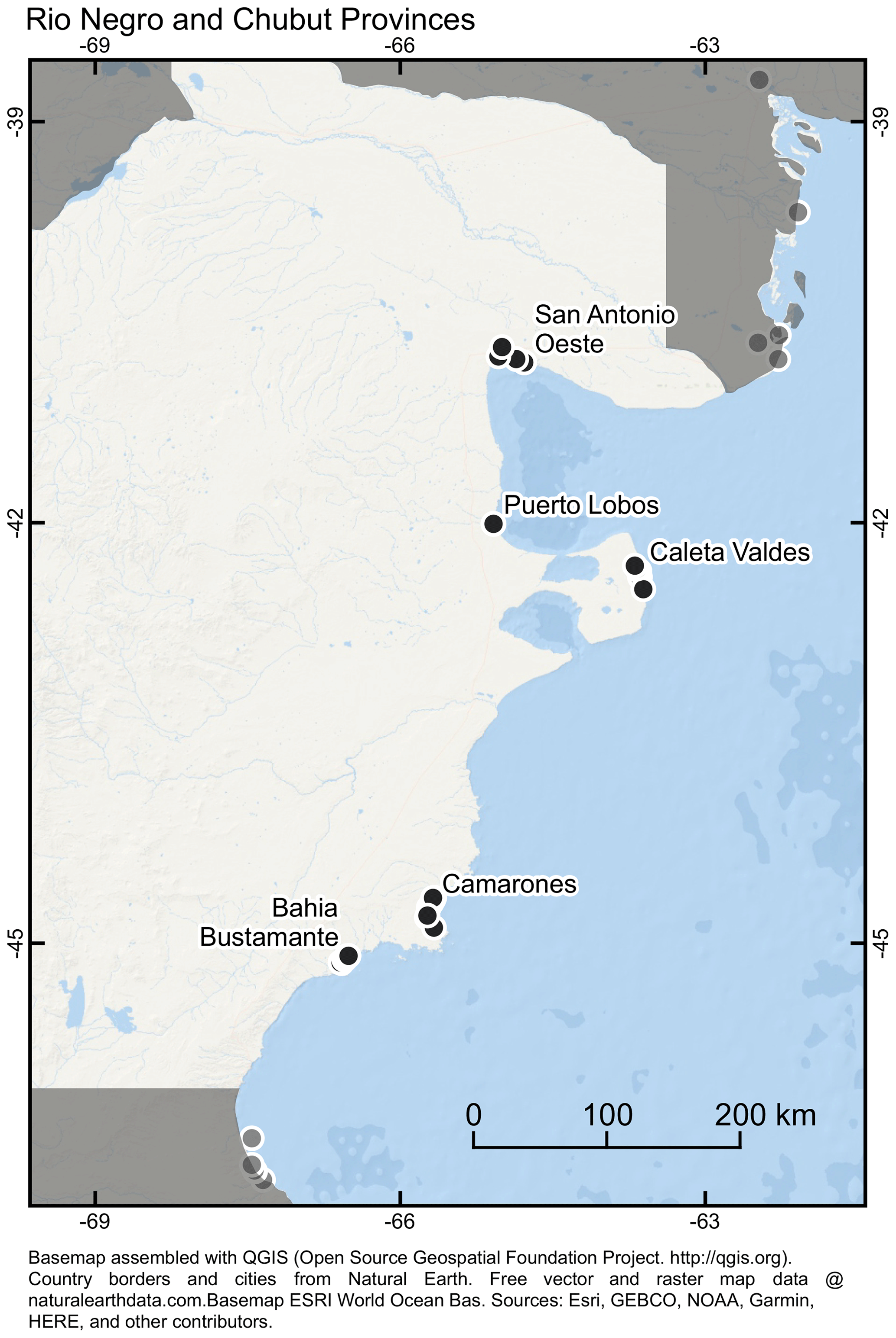
Figure 8 MIS 5 sea-level indicators in Río Negro and Chubut provinces, Argentina (black circles).

San Antonio Oeste

Rutter et al. (1989, 1990) and Radtke (1989) collected mollusc samples at eight locations with beach ridges and beach deposits in the San Antonio Oeste area. Four of these locations, described below, with stated elevations of between 8–12 m, were assigned an MIS 5 age on the basis of AAR values and ESR dates. Fucks et al. (2012b) also visited these sites and provided further descriptions of the geomorphology and mollusc fossils of these deposits.

A section near Baliza San Matías (Faro San Matías in Radtke, 1989) contains a beach deposit (Radtke, 1989; Rutter et al., 1989, 1990). The elevation of the section is inconsistent between the studies. Rutter et al. (1989, 1990) described the section at 11 m a.m.s.l. (without description of what the elevation refers to), with the beach gravel deposit beneath 1.5 m of loess. The sketch in these papers indicates that the section thickness is 4.4 m, with the sample taken from about 2 m below the top of the section. Radtke (1989) described the section as approximately 0.9 m thick, with the top of the beach gravel layer being at about 10 m a.m.s.l., although it should refer to the same section as Rutter et al. (1989, 1990). We have taken the elevation from Rutter et al. (1989, 1990), which has a much broader elevation range and will encompass the range stated in Radtke (1989). Calculated paleo sea level from this location is 9.0 ± 5.5 m.

Another site, at Puerto de Vialidad (Radtke, 1989; Rutter et al., 1989), comprised an 8 m section of beach gravel, described as being at the same elevation as Baliza San Matías and it is unclear whether the elevation refers to the top or bottom of the deposit. The calculated sea level for this location is 9.7 ± 8.5 m.

At a site at La Rinconada there is a 0.5 m section containing beach gravel, which overlies a shore platform. As with the site at Baliza San Matías, there is a discrepancy between the description in Radtke (1989) and in Rutter et al. (1989, 1990). Radtke (1989) states the elevation is about 8 ± 2 m (originally referenced to high tide, corrected assuming the high tide is 5 m). Rutter et al. (1989, 1990) report the elevation as 8–12 m. We use the elevation reported by Rutter et al. (1989, 1990) to be consistent with the other sites at San Antonio Oeste. The sea level from the beach deposit is 8.7 ± 3.9 m, while the shore platform is 8.0 ± 4.8 m.

A site called “Tankstelle” (a gas station) northwest of San Antonio Oeste has beach ridges that were dated with ESR and U∕Th methods (Radtke, 1989). The reported elevation of the beach ridges was 8–12 m in Rutter et al. (1990), while the description in Radtke (1989) merely states “about 12 m”. As with the other locations, we use the description from Rutter et al. (1990). The calculated sea level from this location is 6.3 ± 2.8 m.

5.4 Patagonia – Chubut Province

Chubut Province has data at five locations (Fig. 8).

5.4.1 Puerto Lobos

Bayarsky and Codignotto (1982) investigated six raised shoreline deposits in Puerto Lobos. Mollusc shells from two of the deposits, consisting of beach gravel, had minimum radiocarbon ages. Due to their similar elevation to better-constrained sea-level indicators in the region, we tentatively correlate these deposits to MIS 5. The calculated sea levels of the beach deposits are 8.8 ± 2.9 and 6.8 ± 2.7 m. Pastorino (2000), Aguirre et al. (2008), and Boretto et al. (2013) provided additional information on the mollusc fossils from these deposits. Notably, the deposits attributed to MIS 5e in Puerto Lobos provide the most robust evidence of warmer ocean conditions of any site in Patagonia (Aguirre et al., 2008).

5.4.2 Caleta Valdés

Codignotto (1983) surveyed the surface of a marine terrace on the northern Valdes Peninsula, with an elevation of 20 ± 5 m, measured by barometric altimeter. Marine mollusc shells, in living position, returned finite radiocarbon ages. However, the terrace is considered to be of MIS 5 or older on the basis of elevation. The location of the surveyed landform is only described generally. The sea level from this indicator is 19.1 ± 7.5 m.

Rutter et al. (1989) collected samples of marine mollusc shells for AAR analysis at four of five beach ridges identified at Caleta Valdés. They concluded, based on the relative differences in AAR values of nine shell species (Table 6), that the second-lowest set of ridges with a peak elevation of about 27 m is MIS 5 in age. The elevation range of the beach ridges is estimated from a diagram in the paper and falls between 20 and 27 m, indicating a sea level of 20.7 ± 4.4 m. ESR dating of mollusc shells from this beach ridge confirmed this assignment (Radtke, 1989; Rutter et al., 1990).

Schellmann (1998) reported dates from a lagoon deposit located between the beach ridges attributed to MIS 5 by Rutter et al. (1989, 1990) and another beach ridge that returned an ESR date that was older than 279 ka. The ESR dates from this deposit are consistent with MIS 5 (109–136 ka), but Schellmann (1998) suspected the age was underestimated because the current water saturation conditions are less than what was likely normal for the sediments. They therefore assigned an MIS 7 age. No modern analogue for the lagoon was given in the original study, so we took it to be −1.5 m below the lowest low-tide value, as this is the maximum depth of modern lagoons worldwide (Rovere et al., 2016). If it is an MIS 5 deposit, then the calculated sea level is 9.2 ± 3.3 m.

Rostami et al. (2000) collected mollusc shell samples from two marine terraces. At both sites, they reported the elevation of the top of the terrace and collected the samples at a 1.2 m depth of burial from the top of the terrace. The lower seaward terrace has a calculated sea level of 15.6 ± 4.0 m, while the higher landward one is 16.6 ± 4.2 m. Further details on the morphology of the terrace were not presented.

5.4.3 Cabo Raso

Codignotto (1987) described marine deposits located at 20–22 m at Cabo Raso, with minimum radiocarbon ages. However there is not enough detail to infer a sea-level indicator from their description. Ribolini et al. (2011) reported a beach ridge at Cabo Raso at a 15–16 m elevation, which was assigned a Pleistocene age on the basis of elevation and faunal content. However, no dating of this landform was performed, so it was also not included in our database.

5.4.4 Camarones

Codignotto (1983) surveyed and described possible MIS 5 elevated terraces and beach deposits in the Camarones area. The exact location of these sites is uncertain, but the author describes a 15 km section of coastline near the town. The first site is a beach deposit located north of Camarones. The elevation was taken from Feruglio (1950) and was likely not measured during the survey of Codignotto (1983). The elevation of the deposit was reported as 17–22 m. Shell samples, retrieved from living position, returned minimum radiocarbon ages. Based on elevation, it is possible that it is an MIS 5 deposit. The sea level calculated from this deposit is 19.0 ± 5.4 m. The second site south of Camarones is a marine terrace measured with an altimeter to an elevation of between 15–22 m. Codignotto (1983) did not state what the elevation was referencing. The terrace contained shells in living position. The sea level calculated from this site is 17.8 ± 6.1 m.

Schellmann (1998) and Schellmann and Radtke (2000) described two MIS 5 beach ridges located north of Camarones. The first site (Pa 47) has a calculated sea level of 6.5 ± 5.8 m. Pappalardo et al. (2015) dated this deposit using the U∕Th method on a mollusc shell and confirmed the MIS 5 assignment, but there were not enough details to narrow the vertical uncertainty. The large vertical uncertainty is a result of the thickness of the deposit. Another site with a beach ridge (Pa 30) has a calculated sea level of 12.8 ± 3.3 m, but this should be regarded as lower quality since the geological context was not described.

Rostami et al. (2000) investigated an MIS 5 marine terrace located about 12 km south of Camarones. Since there was no map or coordinates in the paper, we assign a low quality score to this indicator. About 1 m below the surface were shells in living position. The calculated sea level is 15.8 ± 4.0 m.

Pappalardo et al. (2015) described three additional locations that were dated by the U∕Th method with mollusc shells and correlate with MIS 5. Two of these were located north of site Pa 47. The first was a beach ridge, with a calculated sea level of 4.8 ± 5.6 m. The other site, a beach deposit, has a calculated sea level of 6.1 ± 2.4 m. A site south of Camarones was also dated to MIS 5, with a calculated sea level of 7.8 ± 1.5 m. This site is the same as shown in Fig. 4. The later two sites described only the elevation of the shell samples without reference to the thickness of the unit, so these uncertainties are underestimated.

Aguirre et al. (2006) investigated the fauna composition of the shoreline deposits in Camarones. They did not find any significant difference in the fauna content between the deposits attributed to MIS 5 and the Holocene. The interpretation they gave was that there was not a significant difference in the environmental conditions.

5.4.5 Bahía Bustamante

Cionchi (1987) investigated terraces in Bahía Bustamante. These sites are undated, and the terrace surface elevations are estimated from topography maps supplemented by field measurements (measured by altimetry). On the basis of elevation (25–29 m), Cionchi (1987) interpreted the lower of two Pleistocene terraces to represent the last interglacial. If their interpretation of MIS 5 age is accepted, the deposit implies a sea level of 26.4 ± 6.2 m. Rutter et al. (1989, 1990) investigated a beach ridge associated with the marine terrace and, based on amino acid values and ESR dates of mollusc shells, concluded that the beach ridge predates the last interglacial. Therefore, we do not accept the original assignment of an MIS 5 age. Isola et al. (2011) mapped this area, but they did not interpret any marine terraces in Bahía Bustamante and rather show a series of beach ridges. The interpretation of marine terrace landforms being present should be treated with caution.

Schellmann (1998) and Schellmann and Radtke (2000) sampled a number of beach ridge and beach deposits that were interpreted to be MIS 5 in age on the basis of ESR dates. Location Pa 41 has beach deposits, with a calculated sea level of 8.3 ± 2.8 m. Beach ridges at sites Pa 55 and Pa 98 have a calculated sea level of 14.2 ± 3.7 m, but these are regarded as poor quality since there was no stratigraphic context. A beach ridge at site Pa 97 provides a calculated sea level of 5.9 ± 2.3 m, though the ESR dates from this location are somewhat older than MIS 5. Field sites Pa 37, Pa 38, Pa 96, and Pa 95 are located in one beach ridge system. Two well-described outcrops consisting of beach ridge and beach facies within this system provide calculated sea-level values of 12.8 ± 5.6 and 9.5 ± 4.9 m, respectively. Finally, a beach ridge at site Pa 99 has a calculated sea level of 8.3 ± 2.3 m, though this must be regarded as a poor indicator because there are no details given on the outcrop.

Aguirre et al. (2005b) investigated the faunal content of deposits in the Bahía Bustamante area. They found that there was not a significant difference in species found in deposits attributed to MIS 5 compared to the modern species. Therefore, they concluded that there were likely similar environmental conditions.

5.5 Patagonia – Santa Cruz Province

Santa Cruz Province has data at four locations (Fig. 9).

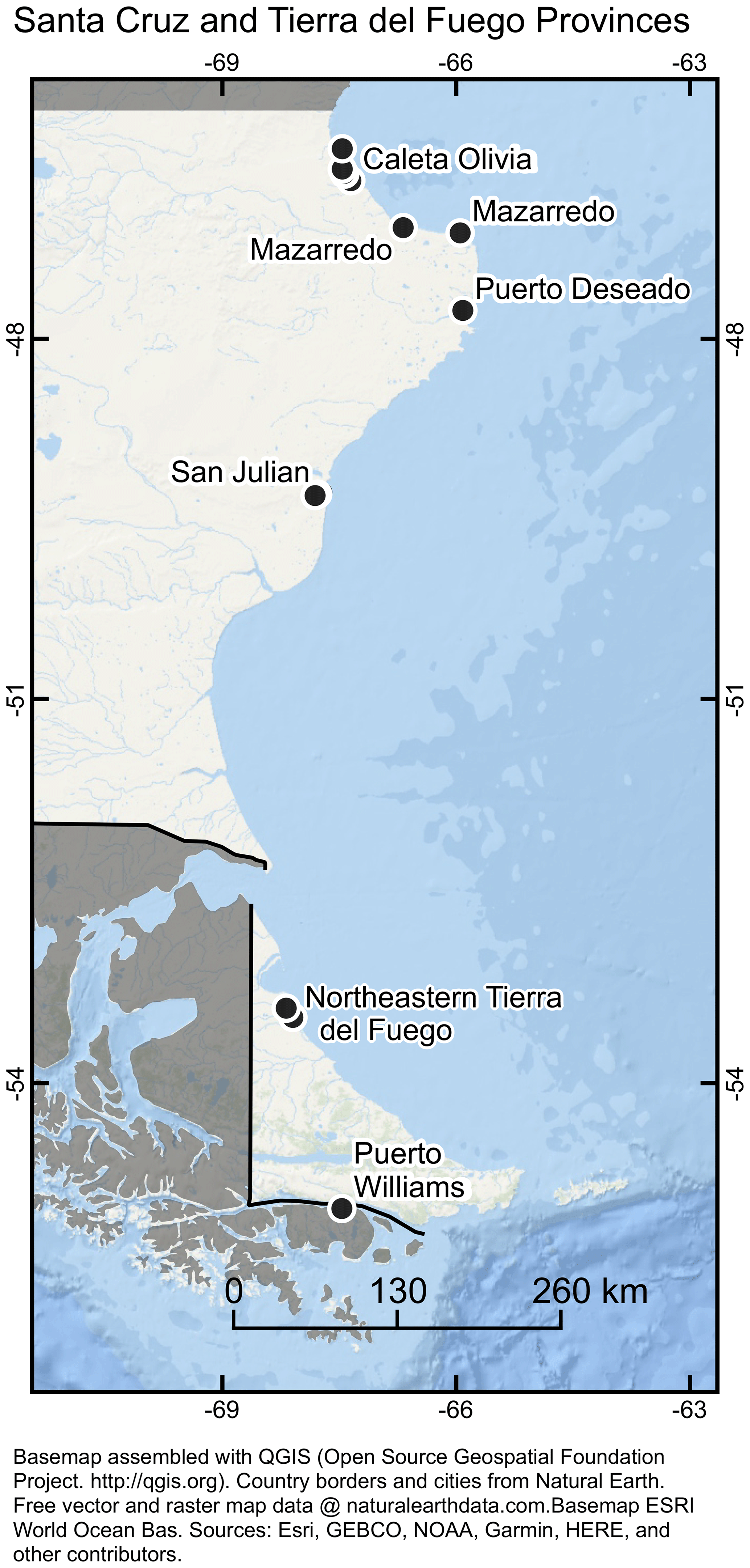
Figure 9 MIS 5 sea-level indicators in Santa Cruz Province, Argentina, and Tierra del Fuego (Argentina and Chile) (black circles).

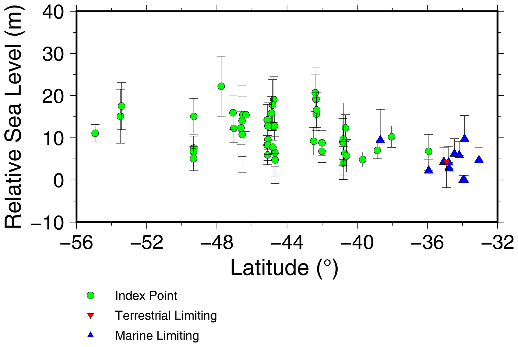
Figure 10 Plot showing the elevation of possible MIS 5 sea-level deposits in southeastern South America.

5.5.1 Caleta Olivia

Codignotto (1983) reported a marine terrace at 12–17 m, which we assume refers to the surface of the terrace, at Bahía Lángara, south of Caleta Olivia, with marine shells in living position associated with gravel deposits. These shells provided minimum radiocarbon ages. The calculated sea level from this site is 12.3 ± 4.0 m.

Schellmann (1998) investigated a beach ridge south of Caleta Olivia. Mollusc shell samples, retrieved from two sample locations 1 km apart, were dated to MIS 5 using ESR dating. Both sites have beach ridge deposits. The site Pa 70 has a calculated sea level of 14.0 ± 8.5 m, while Pa 71 was 10.8 ± 9.0 m. The site Pa 71 is likely the same location that is pictured in Fig. 3. This site was also investigated by Ribolini et al. (2014). They were primarily interested in wedge structures, and a more complete description of the unit is not given.

Rostami et al. (2000) investigated two marine terraces, one north of Caleta Olivia and the other south. Mollusc shells collected from these sites were dated with U∕Th and ESR methods and had MIS 5 ages. Since there is no map, the exact location of these sites had to be estimated based on descriptions of the location in the text. Both terrace surfaces were reported to have the same elevation and have a calculated sea level of 15.5 ± 4.0 m.

5.5.2 Mazarredo

Schellmann (1998) investigated beach ridge deposits at Mazarredo, constraining them to MIS 5 by ESR analysis of mollusc shells. The calculated sea level is 12.2 ± 3.4 m. This indicator is assigned a low quality score, since there was no detailed stratigraphic description of this site.

Rostami et al. (2000) correlated a marine terrace at Punta Mazarredo to MIS 5 using U∕Th dating of a mollusc shell. The calculated sea level is 15.9 ± 4.0 m. The location is described as, “130–150 km from Caleta Olivia” (Rostami et al., 2000, p. 1506). Using satellite imagery, we identified raised shorelines at this approximate distance from Caleta Olivia and have tentatively assigned the location of the sea-level indicator to these coordinates within WALIS. This is about 55 km east of the location described by Schellmann (1998).

5.5.3 Puerto Deseado

Rutter et al. (1989) sampled mollusc shells with AAR from three beach deposits in the Puerto Deseado area from three different elevations. The intermediate elevation deposit, with an elevation stated to be 20–25 m, was interpreted as being last interglacial in age based on relative AAR values. The mollusc samples were taken from the top 3 m of a 4 m thick layer of beach gravel. The sea level calculated from this deposit is 22.2 ± 7.1 m. Rutter et al. (1990) and Radtke (1989) reported ESR dates from this deposit that were minimum limiting (> 415 ka), so they reinterpreted this deposit to be older than the last interglacial.

Several more recent studies have investigated features interpreted as being MIS 5 in age, but since they did not perform additional dating and elevation measurement techniques were not stated, they do not reduce the uncertainty in the entered index point. Bini et al. (2017) reported on the inner margin and an abrasion notch of the marine terrace they correlated to MIS 5, with elevations between 21.4 and 23.4 m. They interpreted these features to represent a paleo sea level of about 21 m. However, these features cannot be directly dated. Zanchetta et al. (2014) reported on a sandy gravel deposit that they correlated to MIS 5e with a peak elevation of 11–13 m, but since they were not marine deposits, they do not narrow down the position of sea level. Ribolini et al. (2014) reported on a marine unit they interpreted as MIS 5 at a site west of the town of Puerto Deseado. Schellmann (1998) appears to have dated this deposit with ESR, which returned non-finite ages and is therefore likely older than MIS 5.

5.5.4 San Julián

Radtke (1989) was the first to present a dated last interglacial shoreline deposit in San Julián. They identify a marine terrace surface at 8–10 m but provide no additional description. The elevation range is exactly the same as what is stated by Feruglio (1950), and we suspect that the elevation was not measured but simply taken from the older publication. ESR dating of mollusc shells from the underlying deposit indicates this terrace is MIS 5 in age. The calculated sea level from this landform is 7.6 ± 3.4 m.

Schellmann (1998) reported MIS 5-aged deposits at two locations. Southwest of San Julián at site denoted as Pa 122 and Pa 123 is a sequence of sublittoral facies, overlain by beach facies, and followed by beach ridge facies that records a sea-level regression. ESR analysis of mollusc shells retrieved from two separate shell layers within the beach ridge facies indicated MIS 5 deposition. The beach facies has a calculated sea level of 6.7 ± 3.8 m, while the overlying beach ridge facies implies a sea level of 5.1 ± 2.9 m. The second location described by Schellmann (1998), Pa 61, is located east of San Julián, but there is not enough information on the stratigraphic context to infer sea level.

Rostami et al. (2000) reported a marine terrace overlying a wave-cut platform, about 2 km south of San Julián. U∕Th dates were consistent with an MIS 5 age. The calculated sea level of the terrace surface is 15.1 ± 4.2 m.

5.6 Patagonia – Tierra del Fuego

Tierra del Fuego, which includes parts of Argentina and Chile, has data at two locations (Fig. 9).

5.6.1 Northeastern Tierra del Fuego, Argentina

Codignotto (1983, 1984) reported a Pleistocene beach deposit near Estancia La Sara to the south-southeast of San Sebastián Bay. They collected several mollusc shell samples which provided minimum radiocarbon ages. The elevation of the deposit was described as 20–22 m, with shells found up to 5 m below the surface. If this is an MIS 5 deposit, the calculated sea level of this deposit is 17.5 ± 5.6 m.

Rutter et al. (1989) sampled a beach deposit near Estancia La Sara that they interpreted as being Pleistocene based on elevated AAR values on mollusc shells relative to Holocene deposits. The samples were taken from a 5 m section of foreshore beach gravel, at a 2–5 m depth of burial below. Meglioli (1992) stated additional, unpublished AAR samples indicated an MIS 5 age. Bujalesky et al. (2001), Bujalesky (2007), and Bujalesky and Isla (2006) collected a U∕Th sample that was consistent with an MIS 5 assignment. They measured an elevation of 14.3 m at the top of this beach deposit using GPS. Their coordinates and site description indicate it was the same location as that of Rutter et al. (1989), but since the stratigraphic details are limited, we apply an additional 1 m of uncertainty to this measurement. The calculated sea level is 13.4 ± 3.7 m.

Bujalesky and Isla (2006) and Bujalesky (2007, 2012) also described Upper Pleistocene gravel beaches in Río Grande, Cabo Peñas, Ensenada La Colonia, and Río Fuego at 6–8 m above the present storm berm and which have an inferred MIS 5 age. These landforms have not been dated, so we do not include them in our database.

5.6.2 Puerto Williams, Isla Navarino, Chile

This beach deposit outcrop is located about 10 km east of Puerto Williams. The deposit is overlain by Wisconsin-aged (post-MIS 5e) glacial till (Rabassa et al., 2008). They noted that beach deposit had not been deformed or displaced by glacial action. A minimum radiocarbon age on a shell fragment was reported. Björck et al. (2021) revisited the site or perhaps another close by since they were unable to find the till unit. They collected IRSL dates that are consistent with an MIS 5 assignment. They remeasured the elevation with a clinometer, but since the benchmark was not stated, it does not improve the uncertainty in the elevation from the previous descriptions. The calculated sea level from this deposit is 11.0 ± 1.5 m. The fossil assemblage of marine molluscs indicates that marine conditions were similar to those in the present (Gordillo and Isla, 2011; Gordillo et al., 2010).

6 Further details on paleo sea level

In this section, we highlight some details on topics of interest to those investigating last interglacial sea level in southeastern South America. Of particular note are the extensive surveys of the faunal content of the shoreline deposits, the existence of Holocene and pre-MIS 5 shoreline deposits that are elevated compared to present sea level, and the debate on why last interglacial sea-level indicators in the study area are elevated compared to low-latitude areas.

6.1 Faunal content

There are extensive surveys of fauna diversity at many MIS 5 sites, including Uruguay (Martínez et al., 2001; Rojas and Martínez, 2016; Rojas and Urteaga, 2011; Rojas et al., 2018b, a), Buenos Aires Province (Aguirre, 1992), Pilar (Fucks et al., 2005), Ezeiza (Martínez et al., 2016), Magdalena (Aguirre and Whatley, 1995), Colorado River delta (Charó et al., 2015), southern Buenos Aires Province (Fucks et al., 2012a), Bahía Blanca (Aliotta et al., 2001), Bahía Anegada (Charó et al., 2013a), San Blas (Charó et al., 2013b, 2018), San Antonio Oeste (Bayer et al., 2016b, a), Río Negro and Chubut provinces (Pastorino, 2000), Santa Cruz Province (Aguirre et al., 2009), the Camarones area (Aguirre et al., 2006), Bahía Bustamante (Aguirre et al., 2005b), Caleta Olivia (Aguirre, 2003), Puerto Lobos (Aguirre et al., 2005a; Boretto et al., 2013), Tierra del Fuego (Gordillo and Isla, 2011; Gordillo et al., 2010, 2013), Patagonia and Tierra del Fuego (Aguirre et al., 2008), and southeastern South America (Aguirre et al., 2011, 2017). Though many of these studies do not add any new sea-level index points, the surveys indicate that environmental conditions in MIS 5 were likely cooler than the Holocene optimum and similar to present conditions in Patagonia. This is in contrast to the Rio de la Plata region in Argentina and Uruguay, which indicates warmer-than-present environmental conditions (Rojas and Urteaga, 2011; Martínez et al., 2016). However, in the absence of precise numerical dating, faunal surveys on their own can only be used to evaluate the paleoenvironmental conditions. Species distribution may be influenced by salinity and geological influences as well as by temperature (Aguirre et al., 2011). Only after thorough and careful evaluation over a region with correlatable deposits do we regard it as a method to distinguish between deposits of different ages. Further details on this topic can be found in Aguirre (1992, 1993) and Aguirre et al. (2011, 2013, 2017). Considering the wealth of faunal data, we foresee the combination of these datasets, along with more securely dated and differential GPS-measured shoreline deposits, to offer a way to provide a detailed comparison of environmental changes and links to sea-level change. If the fauna is in situ, it also provides the possibility of making a link to sea-level position in the estuary and near-shore deposits we have considered to be marine limiting.

6.2 Last interglacial sea-level fluctuations

The last interglacial lasted approximately 15 000 years. The analytical precision of the ESR and U∕Th methods on mollusc shells from deposits attributed to the last interglacial in the study region is thousands to tens of thousands of years. This limits the applicability of these methods for discerning sea-level oscillations within the last interglacial.

6.3 Other interglacials

Many of the studies that investigated and dated MIS 5 shorelines also reported older deposits at higher elevations. Some of these have been correlated to MIS 7, 9, and 11 on the basis of ESR and U∕Th dates (Schellmann, 1998; Rostami et al., 2000; Schellmann and Radtke, 2000; Pappalardo et al., 2015). Pre-Quaternary raised shoreline deposits have been confidently dated in the study area via strontium dating methods, including to the early Pliocene (del Río et al., 2013; Rovere et al., 2020a), late Miocene (Scasso et al., 2001; del Río et al., 2013, 2018), and Miocene–Oligocene (Parras et al., 2008, 2012; Cuitiño et al., 2015b, a).

6.4 Holocene sea-level indicators

No standardized compilation of Holocene sea-level indicators has been completed. However, one is in development (Timothy Shaw, personal communication, 2019). Previous papers that have comprehensively reviewed Holocene sea level for southeastern South America include Martínez and Rojas (2013), Rostami et al. (2000), and Schellmann and Radtke (2010).

6.5 Controversies

Throughout the past 4 decades, there have been a few points of contention on the interpretation of sea-level proxies in southeastern South America. One of the early controversies was on the interpretation of the age of finite-aged radiocarbon dates in Pleistocene deposits and whether they should be considered to be minimum ages (González, 1992; Rutter et al., 1992). The other controversies described here will require more field observations and modelling work to resolve.

6.5.1 Shoreline angles

The review of Patagonian paleo sea level by Pedoja et al. (2011) reported numerous altimetric measurements of shoreline angles. However, precise locations of these shorelines were not provided. Recent attempts by several of us in the field (Evan J. Gowan, Alessio Rovere, Deirdre D. Ryan, Sebastian Richiano) to locate some of these shorelines, using the publication maps as a guide, were unsuccessful. Pappalardo et al. (2019) were also unsuccessful.

6.5.2 Tectonic uplift or glacial isostatic adjustment of southeastern South America shorelines

The Holocene and MIS 5 shorelines in southeastern South America, specifically in Patagonia, are elevated relative to canonical “eustatic” sea-level values. On this basis, some prior authors have assumed that there is at least some tectonic uplift, generally on the order of 0.1 mm per year (Rostami et al., 2000; Pedoja et al., 2011; Pappalardo et al., 2015). In contrast, Rutter et al. (1989), Radtke (1989), and Schellmann and Radtke (2010) proposed that the raised shoreline deposits were the result of glacial isostatic adjustment (GIA), since the Holocene and MIS 5 highstand elevation is similar along the entire coast. González et al. (1988a) regarded Buenos Aires Province to be relatively stable, with the exception of the Bahía Blanca area, though this reasoning is based on finite radiocarbon ages that we regard as minimum ages.

Few studies of GIA have been performed along the Argentinian coastline. Rostami et al. (2000) did calculations at sites along the South American coastline, but that model did not take into account shoreline migration, which means it neglects the loading effect of the flooding of the broad continental shelf off the coast of Patagonia as sea level rose following the Last Glacial Maximum (details of the Patagonian Ice Sheet were not given). Reanalysis by Peltier and Drummond (2002) included the change in loading on the shelf, and they concluded that the effect was not significant. Peltier et al. (2015) compared the calculated sea level along the Argentinian coastline with the ICE-5G and ICE-6G reconstructions, both with and without rotational effects. They concluded that rotational feedback was detectable in the sea-level signal in this region. However, they were only able to match the Holocene highstand with ICE-5G, which was the result of the impact of the thick Laurentide Ice Sheet on the degree-2 Stokes coefficient.

A publicly available ice sheet reconstruction that spans the penultimate glaciation to the present (which includes the last interglacial) does not currently exist. However, it is possible to make inferences about the magnitude of GIA-induced variations in the southeastern South American sea level after the ice sheets reached their present extent in the mid-Holocene. In Fig. 11, we have plotted the calculated sea level from the PaleoMIST model by Gowan et al. (2021) at 7500 and 2500 BP along the entire study area. This model is a global ice sheet reconstruction for the past 80 000 years, including the Patagonian Ice Sheet. Although this model is preliminary in the sense that it has not been directly compared with Holocene sea-level indicators in southeastern South America, it demonstrates that GIA processes alone can explain sea-level highstands that are well above present-day sea level. We show the results using two different Earth models, one with a continental-style Earth rheology and another with a rheology more appropriate for a place undergoing active tectonics. Regardless of the model, it shows that the coast of southeastern South America has large north–south and east–west variations in peak sea level and that the timing of peak sea level may not be consistent along the length of the coast. This could mean that the peak sea-level highstand documented in our database may represent different points in time within MIS 5. Unfortunately, the precision of the dating methods available is not sufficient to test this supposition.

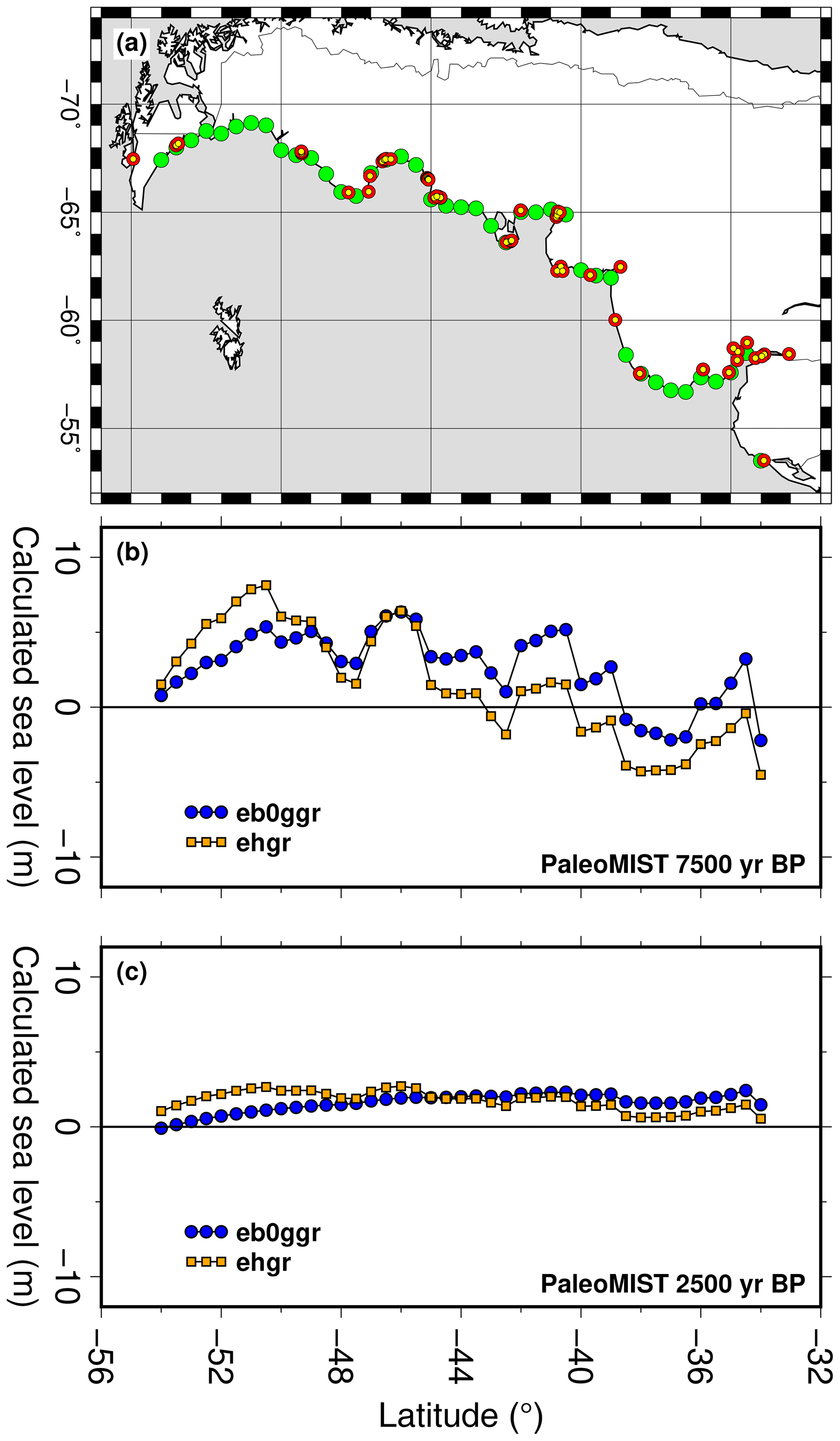
Figure 11 Calculated sea level along the coast of southeastern South America. We use the PaleoMIST ice sheet reconstruction (Gowan et al., 2021) to illustrate the variability in sea level during the Holocene. (a) Map showing where sea level was calculated (green dots) and the location of sea-level indicators described in our database (red dots). Calculated sea level at (b) 7500 BP (approximately when Holocene minimal ice extent was reached) and (c) 2500 BP. The results of calculated sea level with two different Earth models are shown. ehgr (continental-style Earth model): 120 km thick elastic lithosphere, 4 × 10²⁰ Pa s upper mantle and 4×10²² Pa s lower mantle. eb0ggr (tectonically active style Earth model): 60 km thick elastic lithosphere, a 160 km thick layer below that at 10¹⁹ Pa s, 4 × 10²⁰ Pa s upper mantle, and 4 × 10²² Pa s lower mantle.

On longer timescales, tectonics and dynamic topography have affected eastern Patagonia. For example, the Deseado Massif, located in Santa Cruz Province west of Puerto Deseado, was uplifted and tilted after an asthenospheric window in the subducting slab opened due to the northward migration of the Chile Triple Junction (where the Nazca, South American, and Antarctic plates meet) (Guillaume et al., 2009). Most of the tilting and uplift happened from the Miocene to the early Pleistocene. It is unknown if this is still affecting the east coast of Patagonia. Only through additional GIA modelling studies and more precise elevation measurements of MIS 5 shoreline deposits, which is beyond the scope of this study, will it be possible to assess the relative magnitude of these effects.

6.6 Future research directions

The main problem when compiling this database is the lack of precise elevation measurements and references to the indicative range of the landforms. Precise elevation measurements with differential GPS and modern analogues need to be acquired through further field surveys. This would improve the quality of the proxies that have been confidently assigned an MIS 5 age.

One recommendation for future work would be to find an indicative meaning for the Pleistocene deposits that were surveyed in Buenos Aires Province. Specifically, these deposits have been described as estuary deposits, with no indication of the relative water depth in which the deposits formed, making them marine-limiting indicators. If this could be determined, it would provide index points for the entire coast of Argentina. Many of the sites described above have only been dated using minimum radiocarbon ages. Revisiting these sites for additional surveying and better geochronological constraints should be considered for future studies.

7 Data availability

The southeastern South America database is available here: https://doi.org/10.5281/zenodo.3991596 (Gowan et al., 2020). The description of the database fields can be found here: https://doi.org/10.5281/zenodo.3961544 (Rovere et al., 2020b). The information contained in this database was the result of studies from many scientists over the course of several decades. Please cite the original sources of the data in addition to this database.

8 Conclusions

Chronologically constrained and inferred MIS 5 raised shoreline deposits and landforms are located along the entire southeastern coast of South America. The quality of previously published features is generally low, due to the absence of precise elevation measurements, insufficient stratigraphic description or context, and the reliance on radiocarbon dating techniques that can only provide a minimum age constraint to the Pleistocene. Our contribution to the WALIS database should be seen as a starting point to improve measurements of MIS 5e southeastern South American shorelines.