WegenerNet high-resolution weather and climate data from 2007 to 2020

This paper describes the latest reprocessed data record (version 7.1) over 2007 to 2020 from the WegenerNet climate station networks, which since 2007 have been providing measurements with very high spatial and temporal resolution of hydrometeorological variables for two regions in the state of Styria, southeastern Austria: (1) the WegenerNet Feldbach Region, in the Alpine forelands of southeastern Styria, which extends over an area of about 22 km × 16 km and comprises 155 meteorological stations placed on a tightly spaced grid with an average spatial density of 1 station per ∼ 2 km² and a temporal sampling of 5 min, and (2) the WegenerNet Johnsbachtal, which is a smaller “sister network” of the WegenerNet Feldbach Region in the mountainous Alpine region of upper Styria that extends over an area of about 16 km × 17 km and comprises 13 meteorological stations and 1 hydrographic station at altitudes ranging from below 600 m to over 2100 m and with a temporal sampling of 10 min. These networks operate on a long-term basis and continuously provide quality-controlled station time series for a multitude of hydrometeorological near-surface and surface variables, including air temperature, relative humidity, precipitation, wind speed and direction, wind gust speed and direction, soil moisture, soil temperature, and others like pressure and radiation variables at a few reference stations. In addition, gridded data are available at a resolution of 200 m × 200 m for air temperature, relative humidity, precipitation, and heat index for the Feldbach region and at a resolution of 100 m × 100 m for the wind parameters for both regions. Here we describe this dataset (the most recent reprocessing version 7.1) in terms of the measurement site and station characteristics as well as the data processing, from raw data (level 0) via quality-controlled basic station data (level 1) to weather and climate data products (level 2). In order to showcase the practical utility of the data, we also include two illustrative example applications, briefly summarize and refer to scientific uses in a range of previous studies, and briefly inform about the most recent WegenerNet advancements in 2020 towards a 3D open-air laboratory for climate change research. The dataset is published as part of the University of Graz Wegener Center's WegenerNet data repository under the DOI https://doi.org/10.25364/WEGC/WPS7.1:2021.1 (Fuchsberger et al., 2021) and is continuously extended.

1 Introduction

While climate model simulations can achieve kilometer-scale resolution for both general circulation models (e.g., Miyamoto et al., 2013; Klocke et al., 2017) and regional climate models (e.g., Prein et al., 2015; Kendon et al., 2017; Leutwyler et al., 2017; Fuhrer et al., 2018), there is a lack of ground observation data for verifying model outputs and studying weather and climate at this resolution. Common meteorological networks cover scales of 10 km or larger (e.g. interstation distance in Switzerland (of MeteoSwiss-operated rain gauges) is 10–15 km (Wüest et al., 2010), and in Germany the Deutscher Wetterdienst (DWD) operates about 1100 rain gauges (Bartels et al., 2004), resulting in an average interstation distance of about 18 km). At scales below 10 km, most observation networks operate in a campaign-type setting with short observation periods and/or focus on the sub-kilometer scale only (e.g., Moore et al., 2000; Jensen and Pedersen, 2005; Ciach and Krajewski, 2006; Fiener and Auerswald, 2009; Pedersen et al., 2010; Jaffrain and Berne, 2012; Peleg et al., 2013). In the 1950s and 1960s some larger networks existed at this scale, for example in Illinois, USA (Huff and Shipp, 1969), and Oklahoma, USA (Hershfield, 1969), but data from these networks are not in a digital format and are therefore of limited use for current analyses if they are even accessible at all. To the authors' knowledge, only two operational long-term-observation facilities at the 1 to 10 km scale exist worldwide: the Walnut Gulch Experimental Watershed (hereafter just called “Walnut Gulch”), which focuses on rainfall measurements and is located in a semi-arid climate in southeastern Arizona, USA (Goodrich et al., 2008; Keefer et al., 2008), and the WegenerNet Feldbach Region (FBR) climate station network (which is presented in this paper), which provides a broad array of hydrometeorological variables and is located in the southeastern Alpine forelands of Austria (Kirchengast et al., 2014). Walnut Gulch covers an area of about 149 km² and consists of about 90 rain gauges, located at altitudes between 1100 and 2300 m (Tan et al., 2018), resulting in an average density of about 0.6 gauges per square kilometer. In the WegenerNet FBR, 155 hydrometeorological stations are distributed over an area of about 300 km² at altitudes ranging from 257 to 520 m. The average density is about 0.5 stations per square kilometer.

The WegenerNet FBR was specifically built as a long-term weather and climate monitoring facility that would provide open-ended measurements at very high spatiotemporal resolution. It has been in operation since January 2007 and helps fill the gap between short-term, high-resolution observations and long-term observations at larger scales. In 2010, the WegenerNet FBR was expanded with an Alpine sister network. The WegenerNet Johnsbachtal (JBT) covers 13 meteorological stations and 1 hydrographic station in an area of about 16 km × 17 km, with altitudes ranging from about 600 to 2200 m above mean sea level (m.s.l.). A detailed description of both networks can be found in Sect. 3.

This paper focuses on an up-to-date characterization of the two WegenerNet networks. It describes the latest reprocessed data record (version 7.1) over 2007 to 2020 and their processing from raw data (level 0) via quality-controlled basic station data (level 1) to weather and climate data products (level 2). In order to showcase the practical utility of the data we also include two illustrative example applications and briefly summarize and refer to scientific uses in a range of previous studies.

2 Existing literature and previous studies

The WegenerNet FBR was initially described briefly by Kabas et al. (2011b), and a first broader introductory description to the international community was published by Kirchengast et al. (2014). Additional information about the network has been given in several reports. The most comprehensive description of the WegenerNet FBR, including its setup, processing system, and data, is given in the German PhD thesis by Kabas (2012). Subsequent reports focus on specific topics and improvements of the WegenerNet Processing System (WPS): Fuchsberger and Kirchengast (2013) describe the generation of soil moisture data; Szeberényi (2014) focuses on precipitation data analyses, Scheidl (2014) and Scheidl et al. (2017) describe the implementation of new quality control algorithms for precipitation and humidity data, respectively; Ebner (2017) addresses homogenization of temperature and humidity data; and finally Fuchsberger et al. (2018) give an overview of the implemented changes in version 7 of the WPS.

The WegenerNet JBT has been in development for many years and has not yet been described in its entirety in a single paper, although information can be taken from various papers and reports: Strasser et al. (2013) describe 10 of the 14 currently operating stations and a project related to the region, the “cooperation platform Johnsbachtal”. Schlager et al. (2018) give a general description and information about 11 of the 13 meteorological stations, their location, and measured parameters. An MSc thesis by Grünwald (2014) (written in German) contains a detailed description of the Johnsbachtal region, covering its location, geology, and climate as well as providing detailed information about 10 of the 13 meteorological stations. It also includes an overview and analysis of the temperature and wind data collected between 2011 and 2014.

Related scientific output has grown over time, as illustrated by the fact that 11 of 22 scientific journal papers collected as “WegenerNet-related publications” were published in 2018 and 2019. They cover a wide range of topics, including works with a focus on high-resolution rainfall variability and heavy precipitation (Hiebl and Frei, 2018; O et al., 2018; Schroeer and Kirchengast, 2018; Schroeer et al., 2018; Frei and Isotta, 2019; O and Foelsche, 2019), works with a focus on temperature variability and change (Kabas et al., 2011a; Kann et al., 2011; Krähenmann et al., 2011), works with a focus on wind field data and dynamic modeling (Schlager et al., 2017, 2018, 2019), works evaluating precipitation data from radar or satellite measurements (Kann et al., 2015; O et al., 2017; Tan et al., 2018; Lasser et al., 2019; Hu et al., 2020), works with a focus on hydrological modeling of high- and low-flow extremes (Hohmann et al., 2018, 2020), and works with a focus on ecosystem research (Denk and Berg, 2014).

Some of them are directly linked to aspects of the WegenerNet data processing: Schlager et al. (2017, 2018, 2019) focus on the development and evaluation of high-resolution wind fields for both WegenerNet regions, and O et al. (2018) address the validation and correction of rainfall data from the WegenerNet FBR.

A complete up-to-date list of WegenerNet-related literature can be found at https://wegcenter.uni-graz.at/en/wegenernet/publications/ (last access: 14 September 2020).

3 Site description

3.1 WegenerNet Feldbach Region (FBR)

The WegenerNet FBR (Fig. 1a) was established between 2005 and 2006 as a long-term weather and climate monitoring facility, providing measurements at very high resolution (Kirchengast et al., 2014). Its 155 meteorological stations are located in hilly terrain with altitudes ranging from about 250 to 600 m in the southeastern Alpine forelands of Austria, centered near the town of Feldbach (46.938^∘ N, 15.908^∘ E). The stations are spread over a core region (see the heavy black polygon in Fig. 1) with an extent of about 22 km × 16 km and an effective area of about 300 km². The resulting average interstation distance and average station density are about 1.4 km and 0.5 stations per square kilometer, respectively. Station m.s.l. altitudes range from 257 to 520 m (median: 327 m), with 95 % of the stations located below 400 m and only two stations above 450 m. Regular operation started on 1 January 2007, and data from the network are continuously available from this date on.

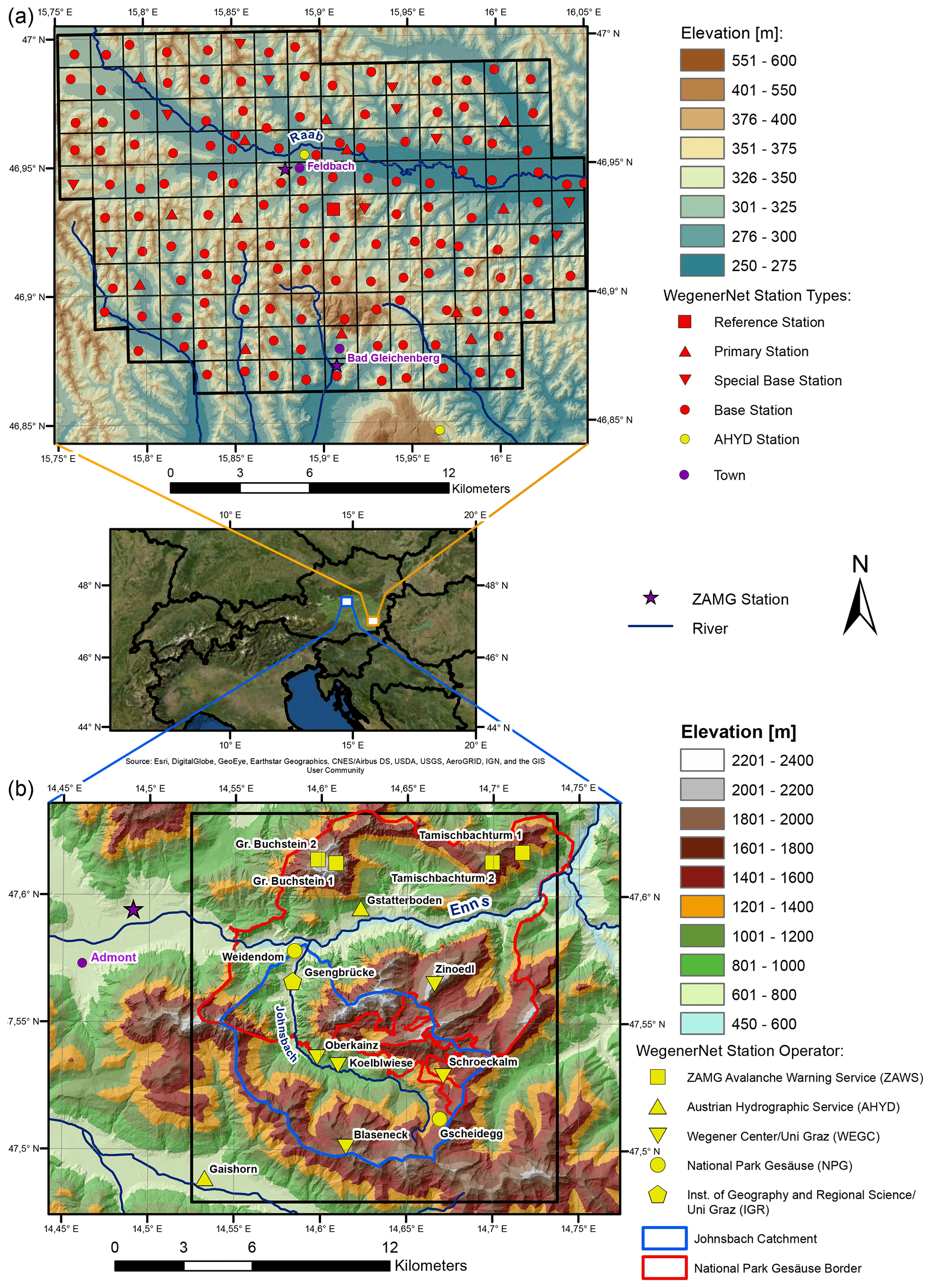
Figure 1 Overview of the study areas: (a) the WegenerNet Feldbach Region (FBR) in the southeast of Styria, Austria, with a core region (thick black polygon) of about 22 km × 16 km and 155 meteorological stations and (b) the WegenerNet Johnsbachtal (JBT) in the north of Styria, Austria, with a core area (black rectangle) of about 16 km × 17 km and 14 stations. The middle panel shows their location in the greater Alpine region (WegenerNet FBR: orange rectangle; WegenerNet JBT: blue rectangle). The legend on the right explains map characteristics, WegenerNet FBR station types (as defined in Table 1), and WegenerNet JBT station operators.

Table 1 Summary of WegenerNet Feldbach Region (FBR) station types, measured parameters, and sensor heights.

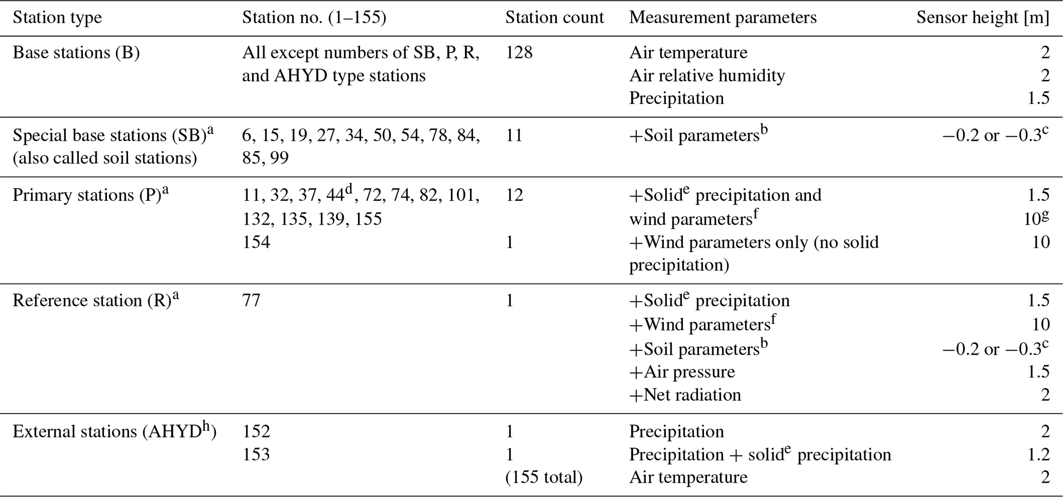
^a Measurement parameters listed for station types SB, P, and R are those that are measured in addition to the B parameters. ^b Soil parameters include soil temperature, soil moisture, pF value, and electric conductivity; see Table A1 for details on installed sensors and Sect. 4 for details on the conversion from pF value to soil moisture. ^c Depth of soil sensors has changed from −0.3 to −0.2 m over the years; see Table A1 for details. ^d Station 44 is a silo rooftop station in the Raab valley measuring temperature and relative humidity at a height of 53 m, precipitation at 51 m, and wind parameters at 55 m. ^e “Solid precipitation” indicates that the corresponding stations are equipped with heated rain gauges and can therefore measure snow and other forms of frozen precipitation in addition to liquid precipitation. Note that for reasons of simplicity liquid precipitation is referred to as just “precipitation” in this table. ^f Wind parameters comprise speed, direction, gust speed, and gust direction. ^g Wind sensor heights for stations 44, 72, and 101 are 55, 18, and 14 m, respectively. ^h Stations operated by the Austrian Hydrographic Service (AHYD).

The region is traversed by the Raab river, which crosses from northwest to east, forming the Raab valley. The main types of land use are agriculture and forestry, with higher fractions of urban fabric along the Raab valley and in the areas of a couple of smaller towns (Schlager et al., 2017, Fig. 2a therein). Information about the region's climate is summarized in Kirchengast et al. (2014) and Schlager et al. (2017).

The stations are grouped into five station types (base, special base, primary, reference, and external stations), each with different instrumentation (Table 1). Besides air temperature, relative humidity, and precipitation, which are measured at most stations, wind parameters, soil parameters, radiation, and air pressure are measured at selected sites. The temporal sampling rate for all parameters is 5 min, except for pF value and soil temperature measured by GeoPrecision sensors, which measure at 30 min intervals. Additionally, since 2018, all parameters measured at special base stations, primary stations, and the reference station sample raw data at 1 min intervals but are later resampled to 5 min in the level 2 (L2) data processing (see Sect. 4).

Table 2 Characteristics of the WegenerNet Johnsbachtal (JBT) stations.

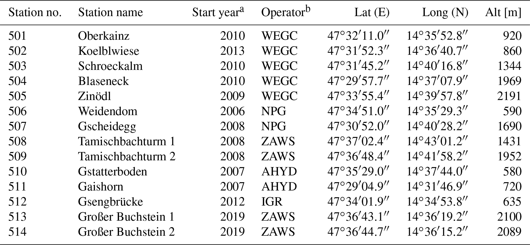
^a Start year of time series (concerning station 506, the first year in the WegenerNet archive is 2007). ^b WEGC: Wegener Center for Climate and Global Change; NPG: National Park Gesäuse; ZAWS: ZAMG Avalanche Warning Service (operated by the Central Institute for Meteorology and Geodynamics (ZAMG) in cooperation with the federal railways company ÖBB); AHYD: Austrian Hydrographic Service; IGR: Institute of Geography and Regional Science, University of Graz.

A detailed list of all installed sensors, their record period, height or depth, and measurement interval can be found in Table A1. For simplicity, we do not give the exact day of installation in this table but only the year. For a detailed overview of the exact installation dates and times, please refer to the WegenerNet data portal (http://www.wegenernet.org, last access: 20 January 2021): navigate to Station Data → Stations → Sensor Details, or download the information in comma-separated values (CSV) format at Station Data → Download → Sensor list CSV file. In the Station Data → Download section of the portal, you can also find a list containing the station coordinates (Station list CSV file) and the sensor specifications of all available instruments (Sensor specs CSV file).

Table 3 Measured variables^a (top row) of the WegenerNet Johnsbachtal (JBT) stations and corresponding sensor heights (numbers in the table).

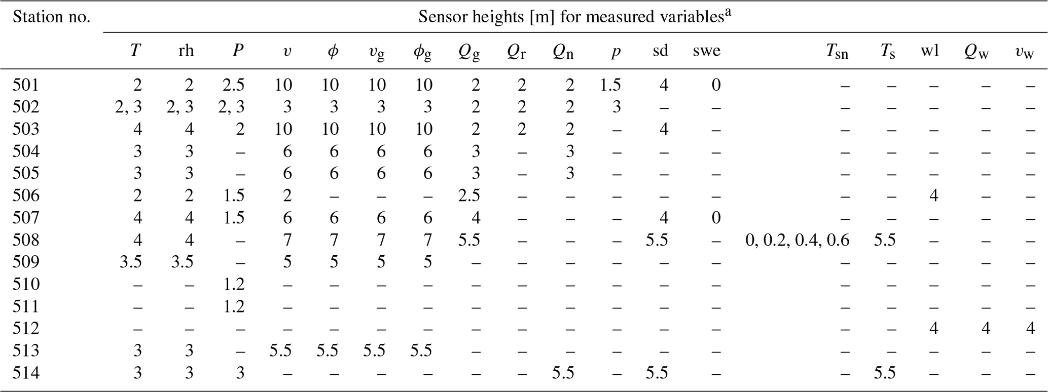
^a T: air temperature; rh: relative humidity; P: precipitation; v: wind speed; ϕ: wind direction; v_g: peak gust; ϕ_g: peak gust direction; Q_g: global radiation; Q_r: reflected radiation; Q_n: net radiation; p: air pressure; sd: snow depth; swe: snow water equivalent; T_sn: snow temperature; T_s: surface temperature; wl: water level; Q_w: water discharge; v_w: water flow velocity; dash (–): variable not measured.

3.2 WegenerNet Johnsbachtal (JBT)

The WegenerNet JBT (Fig. 1b) is an Alpine extension to the WegenerNet FBR and has grown out of the interdisciplinary cooperation platform Johnsbachtal (Strasser et al., 2013). It is situated in the mountainous area of the Ennstal Alps, which are part of the northern Limestone Alps in the north of Styria, Austria. Within a core region of about 16 km × 17 km, 13 irregularly distributed meteorological stations and 1 hydrographic station are located at altitudes ranging from 580 to 2191 m.

The landscape of this region is dominated by limestone mountains (highest peak: Hochtor, 2369 m), steep slopes, and deep valleys, with the Enns river traversing it from west to east through the 16 km long “Gesäuse gorge”. The Johnsbach valley (German: Johnsbachtal) is located as a sub-catchment south of the Enns and lies in the center of the study region (location of Johnsbach village: 47.54^∘ N, 14.58^∘ E). The region also overlaps with the National Park Gesäuse (NPG), one of the six Austrian national parks. The main land use types are forestry and rangeland, with barren land around the limestone peaks and without significant urban settlements in the core region (Schlager et al., 2018, Fig. 2a therein). Information about the region's climate is summarized in Schlager et al. (2018, Sect. 2 therein).

The WegenerNet JBT contains 14 stations, which are operated by different organizations: 6 stations are operated by the University of Graz (5 by the WEGC and 1 by the IGR¹), 4 stations are operated by the ZAMG² avalanche warning service (ZAWS) in cooperation with the federal railways company ÖBB³, 2 stations by the NPG, and 2 stations by the Austrian Hydrographic Service (AHYD).

In 2014, all WEGC-operated stations were added to the WegenerNet facilities infrastructure, and data from these stations were incorporated into the WPS data processing. Over several years, stations from the other providers in the region were gradually added to the network as well once both the data exchange contracts and the long-term access to the actual data had been finalized. A complete list of the station characteristics can be found in Table 2.

Table 4 Overview of the WegenerNet Processing System (WPS) tasks and its different levels of output data. (Task descriptions are written in non-italic text, whereas output data descriptions are italicized.)

The instrumentation differs from station to station and includes sensors for air temperature, relative humidity, precipitation, wind parameters, snow parameters, radiation parameters, air pressure, and hydrographic parameters. A list of all measured parameters at each station, together with the sensor heights, can be found in Table 3. Some of the data are available from 2007 and others only from subsequent years (depending on the individual station's construction dates). The sampling interval is 10 min at all stations except WEGC stations (as of October 2019, when the interval was changed in connection with an upgrade of the data logger hardware) and AHYD stations, where the sampling interval is 5 min. At the NPG stations, the sampling interval was 30 min between 2007 and 2014. See Table A2 for a complete list of all installed sensors including their record period, height, and sampling interval. Just as for the WegenerNet FBR, we do not give the exact day of installation in this table but only the year. For a detailed overview, which is timed down to the hour, please refer to the Station Data → Stations → Sensor Details and Station Data → Download → Sensor list CSV file sections in the WegenerNet data portal (http://www.wegenernet.org, last access: 20 January 2021).

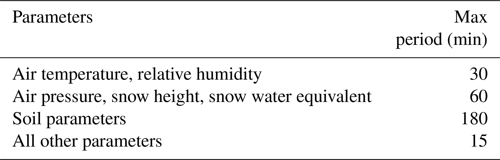
Table 5 Maximum bridged interpolation period of linearly interpolated data in the WPS data product generator (DPG).

4 Data processing and monitoring

The acquisition, processing, and visualization of the stations' data are conducted automatically by the WegenerNet Processing System (WPS), which was originally introduced by Kabas (2012) and Kirchengast et al. (2014). Each release of the WPS is assigned a new version number in order to ensure that the data produced with different releases can be archived and reproduced if needed. The data described in this paper were generated using version 7.1 of the WPS. Table 4 shows an overview of the steps involved in the processing and defines their output products. The WPS consists of four main parts, which are described in the following sections. Except for the proprietary software provided by the data logger manufacturers, the WPS was developed entirely by the WEGC, using Python as the primary programming language and PHP and JavaScript for some parts where using Python was not feasible.

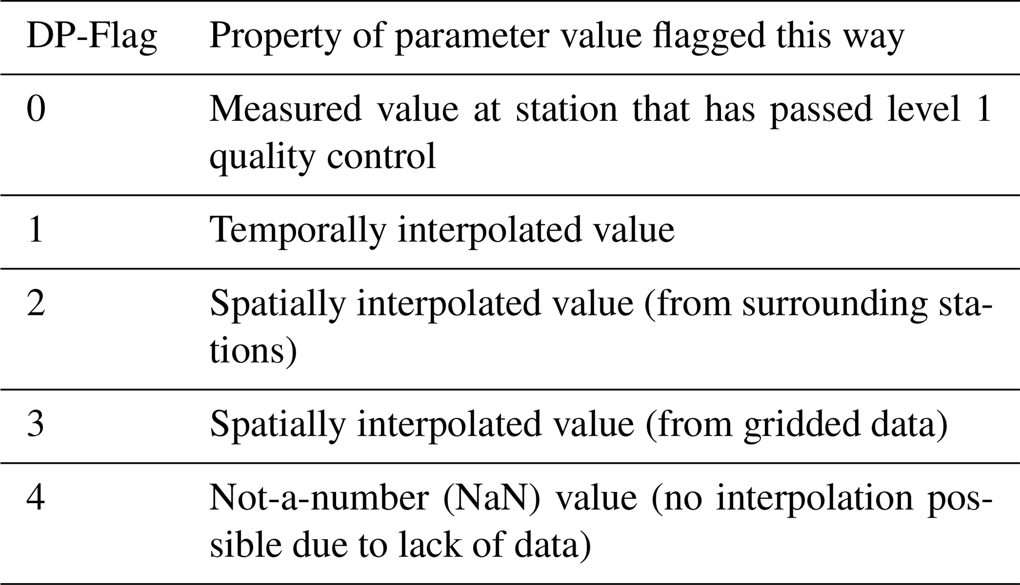
Table 6 Data product flags for level 2 basis data and corresponding properties.

4.1 Level 0 processor: Command Receive Archiving System (CRAS)

In the first processing step, raw data generated by the stations' data loggers are received and stored into a database by the CRAS.

In order to achieve this, the following tasks are executed:

1. The data loggers in the field collect measurements at the sampling interval specified in Tables A1 and A2.

2. Once per hour, the data are sent to the WegenerNet server at the University of Graz.

3. A script reads and writes the data into the WegenerNet PostgreSQL database, producing the so-called level 0 (L0) data.

Additionally, logger and sensor parameters can be changed remotely using the software packages provided by the data logger manufacturers. All relevant metadata like station locations, logger configuration, and sensor details are also stored in the database and can be changed by the WegenerNet team using a comprehensive user interface.

4.1.1 WegenerNet Monitoring and Issue Tracking System (WMITS)

Running as an independent process, the WegenerNet Monitoring and Issue Tracking System (WMITS) screens the incoming data and processing log files at hourly intervals for anomalous values, calculates daily statistics about the data quality, and informs the WegenerNet team by a series of emails containing all the relevant information.

Another part of this task is the automatic surveillance of all heated precipitation gauges. These gauges have additional hardware such as temperature and heating-fan rotation sensors to monitor the proper functioning of the heating system. In case of a detected malfunction, the corresponding sensor is automatically marked as not-heated in the database, and the WegenerNet team is informed by email and can thus initiate immediate actions to remedy the problem. The last part, humidity sensor problem detection, focuses on the issue that humidity sensors are known to be the most error-prone in the network. If the sensor surface is contaminated by dust and dirt, a specific faulty behavior shows a negative offset at high humidity levels, which gets worse as contamination increases and finally results in an inverse measurement of the values. This behavior and its detection are described in detail in Scheidl et al. (2017). The algorithms presented therein have been implemented in the WPS, which enables the early detection of problematic humidity sensors and the reliable posterior flagging of bad sensors.

4.2 Level 1 processor: Quality Control System (QCS)

The QCS checks the data for their technical and physical plausibility and flags all values that did not pass a certain check. It is run hourly and processes all data that are new since the last run. The process analyzes single measurement values and up to 3-hour periods thereof.

Each release of the QCS is assigned a new version number in order to ensure that the data produced with different releases can be archived and reproduced if needed. The data described in this paper were generated using version 5 of the QCS, generating level 1 (L1) data version 5. The QCS consists of seven main processing steps (called QCS layers), which are described in detail in the following paragraphs.

Each layer contains one or several QCS algorithms, called rules, and each rule can set a quality flag (QF) if a check has not been passed. The QFs are unique for each layer in order to ensure that flags issued in different layers can be combined. The code used for encoding the QFs is a simple binary 8 bit integer following the equation

$$\begin{array}{}\text{(1)}& \mathrm{QF}\left(n\right)={\mathrm{2}}^n,\end{array}$$

with n being the number of the respective QCS layer. Thus a QF in layer 0 gets an integer value of ${\mathrm{2}}^{\mathrm{0}}=\mathrm{1}=$ binary 0000 0001, layer 1 gets ${\mathrm{2}}^{\mathrm{1}}=\mathrm{2}=$ binary 0000 0010, layer 2 gets ${\mathrm{2}}^{\mathrm{2}}=\mathrm{4}=$ binary 0000 0100, etc. An example for a combination of QFs would be 0111 0000 (integer ${\mathrm{2}}^{\mathrm{4}}+{\mathrm{2}}^{\mathrm{5}}+{\mathrm{2}}^{\mathrm{6}}=\mathrm{112}$), which would result from failed QCS checks in layers 4, 5, and 6.

If there are insufficient data for executing a certain rule, the respective data values are marked by a so-called no-ref flag instead of a QF. Finally, after a layer has been processed, a checked flag is set. All flags follow the same encoding as described above. The output of the QCS, the L1 data, consists of the L0 data values plus quality flags, no-ref flags, and checked flags.

All checks are executed for each station of the network and for each sensor that is mounted on the station.

• Layer 0 (operations check) checks if a certain station or sensor is in operation (status set manually by the maintenance crew) and sets QF(0) if not.

• Layer 1 (availability check) checks if data from a certain sensor are available and sets QF(1) if not.

• Layer 2 (sensor check) checks if data values lie within the sensor's technical specification and sets QF(2) if not.

• Layer 3 (climatological check) checks if the data values lie within specified climatological bounds and sets QF(3) if not. The bounds are defined for each month of the year and were initially derived from ZAMG climate data maximum and minimum values. Since their initial setup, they have been and still are frequently evaluated using WegenerNet and ZAMG data and adapted when necessary.

• Layer 4 (time variability check) checks for too high or too low variation in the data. It consists of three rules: the first one (gradient check) checks for too large gradients, the second one (constancy check) checks for too low variation, and the third one (pulse check) checks for unnatural spikes. Currently the pulse check is implemented for wind and temperature data only (specifically the wind spike check, described in Sect. 3.1.1 of Fuchsberger et al., 2018, and the temperature spike check, described in Sect. 4.2.1 below). If any of the checks fail, QF(4) is set.

• Layer 5 (intrastational check) checks for meteorological and physical consistency of the sensor values measured at the same station. It consists of six rules: the first one (temperature–precip check) checks unheated rain gauges for precipitation measurements at an hourly mean temperature below 2 ^∘C. Flagging all potential snowfall at unheated stations, it has major implications for the precipitation data in winter since it reduces the effective number of precipitation gauges from 155 to 14 at temperatures below 2 ^∘C.
  The second rule (reference–precip check) checks for consistency between the measurements of the three precipitation gauges installed at the reference station. In the third to sixth rules (windsensor-, wind-mean-boe-, windvalues-, and windboe-dir check), wind data are screened for inconsistencies. For example, the data must satisfy gust value > speed value and gust value and direction ≠ speed value and direction. If any of the checks fail, QF(5) is set.

• Layer 6 (interstational check) deals with the consistency of measurements between a station and its neighbors.

  Neighbor stations for comparison are selected according to the parameter's requirements; e.g. precipitation is compared to the neighbors within a 3 km radius, and temperature and humidity data neighbors are selected according to the altitude difference, location of the stations, and their distance.

  The interstational check comprises seven rules: the first one (maxdiff check) checks for large deviations between the data values of a station and those of its neighbors; the second one (flush check) checks the precipitation data for flushes (sudden opening of blocked funnels or manual flushing by maintenance crew); the third and fourth rules (total blockage check and partial blockage check) check explicitly for (partially) blocked precipitation gauge funnels. The fifth rule (fade away check) checks for the slow, drop-wise emptying of partially blocked precipitation gauge funnels; the sixth one (combined parameter check) checks the combination of temperature and humidity at a single station compared to its neighbors in order to find suspicious values in the humidity data; and the seventh rule (problem flanks check) checks for inverse measurement of humidity sensors. For further details regarding the combined parameter check and the problem flanks check see Scheidl et al. (2017). Further details on the other rules can be found in Scheidl (2014).
  If any of the checks fail, QF(6) is set.

  This layer is applied to WegenerNet FBR data only because the WegenerNet JBT station density is too low for the interstational checks to run reliably.

• Layer 7 (external reference check) compares air pressure and humidity data between ZAMG and WegenerNet FBR stations. If the data deviate too much, QF(7) is set.

  This layer is applied to WegenerNet FBR data only because ZAMG stations near the WegenerNet JBT region are too distant from the other stations.

4.2.1 Temperature spike check

Since some of the EE08-05 temperature sensors that were installed in the WegenerNet FBR in 2018 have been found to produce unnatural spikes in the measurement data, a new check was implemented to detect these spikes. This temperature spike check compares the spike magnitude T_s to the derivative of the (non-flagged) temperature values of the last 120 min before the spike occurred. Figure 2 shows an example of such spikes and those detected by the spike check.

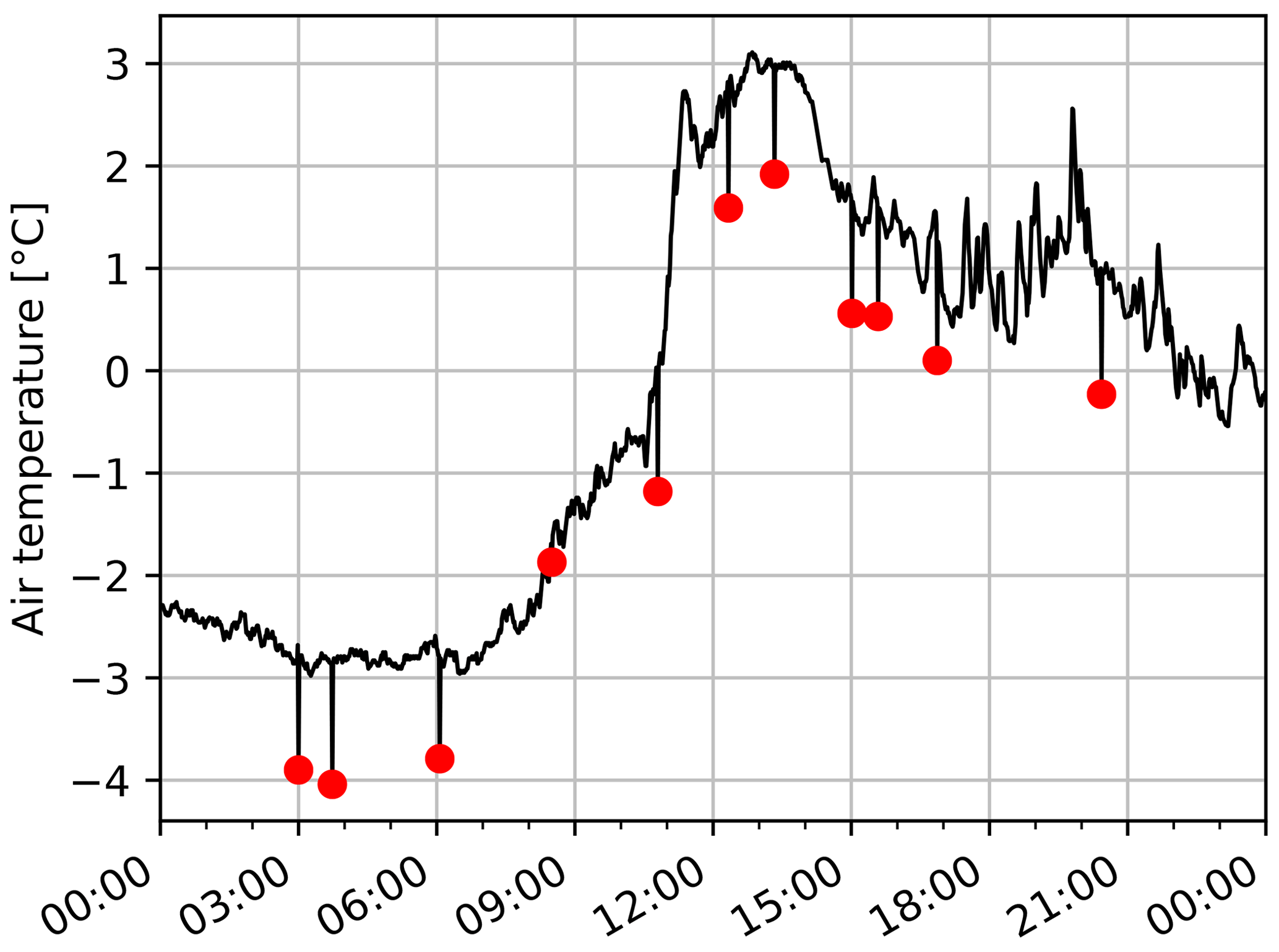
Figure 2 Air temperature data at station 6 on 7 December 2019, showing unnatural spikes. Data points that are flagged by the temperature spike check are marked by red circles.

The check flags any temperature value T_s,i if

$$\begin{array}{}\text{(2)}& T_{\mathrm{s},i}>\mathrm{5}\times \text{SD}\left({\displaystyle \frac{\mathrm{d}{T}_j}{\mathrm{d}t}}\right),\end{array}$$

where T_s is the spike magnitude, and T_j is the (non-flagged) temperature values of the last 120 min (nominally 24 data values).

Note that this check is only executed for sensors that are manually marked as problem sensors by the WegenerNet team.

4.3 Level 2 processor: Data Product Generator (DPG)

The DPG processes all unflagged L1 data (i.e. the best-quality data) and interpolates the gaps resulting from flagged time steps using three different interpolation schemes. It also generates gridded fields of temperature, humidity, and precipitation data for the WegenerNet FBR. The DPG is run hourly after the QCS has finished writing the L1 data.

Each release of the DPG is assigned a new version number in order to ensure that the data produced with different releases can be archived and reproduced if needed. The data described in this paper were generated using DPG version 7, generating level 2 (L2) basis data version 7. The term basis data refers to the temporal resolution (base period) of the L2 data, which is 5 min for the WegenerNet FBR and 10 min for the WegenerNet JBT. Level 2 basis data are generated in near-real time with a data latency of less than 2 h between measurement and storage into the database.

The DPG consists of six main processing steps, described in detail below.

1. On reading the L1 data, the DPG applies homogenization factors for temperature and humidity data according to Ebner (2017).

   Furthermore, precipitation measured by Friedrichs 7041 and Young 52202 sensors is corrected by general correction factors of 1.10 and 1.13, respectively, according to O et al. (2018), and precipitation measured by METEOSERVIS MR3 and MR3H sensors is corrected dynamically by applying the correction curve published in METEOSERVIS (2008).

2. In the second processing step, data with a higher temporal resolution than the region's base period are resampled, generally by averaging (except summation for precipitation, vector mean for wind speed, and maximum for peak gust).

3. The next step is the interpolation of the data gaps. The type of interpolation depends on the length of the interpolation period and the measured parameter; if a gap is shorter than the value defined in Table 5, the missing values are interpolated linearly between the two adjacent valid data values, and a data product flag (DP-Flag) of 1 is set for the interpolated time steps (see Table 6 for definition of DP-Flags).

   Due to the high station density of the WegenerNet FBR, interpolation can also be carried out spatially for the main parameters air temperature, humidity, and precipitation, which are measured at all stations. If a gap is longer than defined in Table 5, the values for temperature and humidity are interpolated from the values of the surrounding stations using a linear-inverse-distance-weighting (IDW) algorithm. The temperature values are projected to a reference altitude of 300 m before interpolation using a lapse rate calculated from all stations' temperature data and their altitudes for every 1 h time window. Precipitation data are interpolated using an inverse-distance-squared-weighting (IDSW) algorithm. Further, a DP-Flag of 2 is set for all neighbor-station-interpolated data.

4. In the fourth step, 200 m × 200 m, 5 min resolution gridded fields of air temperature, humidity, and precipitation are generated for the WegenerNet FBR. The fields are calculated by interpolating the station measurement values onto the grid using the same algorithms as described in step 3 (IDW for air temperature and humidity, IDSW for precipitation). Additionally, the spatial maximum, minimum, average, and standard deviation are calculated for all gridded fields. Temperature grids are stored in three separate fields, one calculated at a constant reference altitude of 300 m and two terrain-following fields. For these two fields, one is calculated at the average terrain altitude of each grid point and one at the altitude of the center of each grid point. In this context a digital elevation model (DEM) with 10 m resolution is used for calculating the altitudes. The altitude dependence of the temperature is accounted for by using the calculated lapse rate as described in step 3.

   The DP-Flags of the fields are also stored as 2D grids, serving as spatially resolved quality indicators. The DP-Flag values of each station are interpolated onto the grid using the same interpolation algorithm as for the corresponding measurement values. Additionally, the spatial average of each DP-Flag grid is calculated. Two examples of gridded DP-Flag data can be found in Fuchsberger et al. (2018, Fig. 2.1 therein).

5. WegenerNet FBR air temperature, humidity, and precipitation data that could not be interpolated from the surrounding stations in step 3 are then interpolated from the gridded data calculated in step 4. Temperature data are interpolated from the reference altitude (300 m) grid and then projected back to the stations' altitudes using the lapse rate calculated in step 3. Furthermore, a DP-Flag of 3 is set for the interpolated time steps.

6. If a gap could not be interpolated, the missing time steps are filled with an empty value (not a number, NaN) and are marked by a DP-Flag of 4.

4.4 Level 2+ processor: wind products and value-added products

The L2+ processor generates data derived from several input variables, including one or several L2 data variables and other sources like soil texture data, land use data, etc. It is run hourly after the DPG processing has finished.

4.4.1 Wind Product Generator (WPG)

The WPG generates high-resolution 100 m × 100 m wind fields and peak gust fields for the WegenerNet FBR and WegenerNet JBT using the California Meteorological Model (CALMET) as a core tool. It is run hourly after the DPG processing has finished and was derived in recent years by Schlager et al. (2017, 2018). Input variables of the model are meteorological observations, terrain elevations taken from a 100 m resolution DEM, and land use information. Meteorological variables include temperature, air pressure, wind speed, and wind direction, all taken from WegenerNet station observations. The wind fields are generated for two height levels (10 m and 50 m above ground) with a temporal resolution of 30 min.

Gust fields are generated for a height of 10 m above ground in a separate process described in Schlager et al. (2018, Sect. 3.3 therein). Since the publication of this study, the gust field generation was further refined by changing the IDW algorithm mentioned therein to an IDSW algorithm and by limiting the maximum gust values of a time step to the maximum gust speed of all stations, multiplied by a factor of 1.2 to allow moderate overshooting. This helped to reduce unnaturally high gust speed values that can occur if the ratio between gust speed and average wind speed varies strongly between stations.

Detailed information about the WPG can be found in Schlager et al. (2017) and Schlager et al. (2018), and a comparison with other models for both regions was made by Schlager et al. (2019).

Similarly to the QCS and DPG, the releases of the WPG are versioned for each new release. The version used for generating the described data is WPG v7.1.

4.4.2 Value-Added Product Generator (VAPG)

The VAPG generates data derived from L2 data and complementary data sources. It currently contains two main processing steps.

Soil moisture data generation

Soil moisture time series data are derived from L2 pF value data and soil-related metadata like soil texture, humus content, and dry bulk density using the Mualem–van Genuchten equation (Mualem, 1976; van Genuchten, 1980). A detailed description of this process can be found in Fuchsberger and Kirchengast (2013).

The pF values were the only source of information about soil moisture in the WegenerNet FBR until 2013, when replacement of pF meters by Stevens HydraProbe II sensors (capable of measuring soil moisture directly) began. Since then, pF meters at all soil stations have been replaced or supplemented by HydraProbe II sensors (see Table A1 for details on the sensor mount dates). For keeping a cross-comparison capacity, stations 27 and 77 have both types of sensors installed.

Heat index data generation

Gridded heat index (apparent temperature) fields are generated from L2 temperature and humidity fields using an equation developed by Schoen (2005),

$$\begin{array}{}\text{(3)}& \mathrm{HI}=T-\mathrm{1.0799}{e}^{\mathrm{0.03755}T}\left[\mathrm{1}-e^{\mathrm{0.0801}(D-\mathrm{14})}\right]\text{,}\end{array}$$

where HI is the heat index (^∘C), T the air temperature (^∘C), and D the dew point (^∘C).

The dew point therein is calculated using an equation based on the Magnus–Tetens formula (Barenbrug, 1974; Schoen, 2005):

$$\begin{array}{}\text{(4)}& D={\displaystyle \frac{b\times \mathit{\alpha }}{a-\mathit{\alpha }}}\text{,}\end{array}$$

where $\mathit{\alpha }=\frac{a\times T\left[{}^{\circ }\mathrm{C}\right]}{b+T\left[{}^{\circ }\mathrm{C}\right]}+\ln \left(\mathrm{RH}\right)\text{,}$ a=17.27, b=237.3, and RH is the relative humidity expressed as a (dimensionless) fraction between 0 and 1.

As an auxiliary classification, for user convenience, the heat index is also categorized into a scheme of five danger classes (based on NOAA, 2020), consisting of comfortable (20 ^∘C < HI < 27 ^∘C), caution (27 ^∘C < HI < 32 ^∘C), extreme caution (32 ^∘C < HI < 41 ^∘C), danger (41 ^∘C < HI < 54 ^∘C), and extreme danger (HI > 54 ^∘C).

4.5 Level 2 products processing: Weather and Climate Products Generator (WCPG)

4.5.1 Data aggregation

All L2 data, including value-added data products, are aggregated to half-hourly, hourly, and daily (weather data) and monthly, seasonal, and annual (climate data) products. The aggregation is generally done by averaging the data, with the exception of wind speed and direction (the vector mean is used for consistent averaging), peak gust data (the maximum value is used), and precipitation data (the sum is taken). For temperature data, the maximum and minimum values are also calculated. Weather data are generated by aggregating the basis data, and climate data are generated by aggregating the daily data.

4.5.2 Weather and climate data quality indicators

A special algorithm is used for calculating quality indicators for weather and climate data, the so-called flagged percentage of data (FP). The FP indicates how many of the data have been interpolated or flagged as missing in the DPG, but it does not indicate how the data have been interpolated (i.e. which DP-Flag they have received). It is calculated for station time series data using the following equations (taken from Fuchsberger et al., 2018).

• a.

  For continuous data, like temperature and humidity:

  $$\begin{array}{}\text{(5)}& {\mathrm{FP}}_c={\displaystyle \frac{N[\text{DP-Flag}>\mathrm{0}]}{N_{\mathrm{total}}}}\cdot \mathrm{100}\left[\mathit{\%}\right],\end{array}$$

  where N[DP-Flag>0] is the number of flagged basis data values, and N_total is the total number of basis data values within the given time span of a weather or climate data product.

• b.

  For precipitation data,

  $$\begin{array}{}\text{(6)}& {\mathrm{FP}}_P={\displaystyle \frac{P_{\mathrm{flagged}}\left[\mathrm{mm}\right]}{P_{\mathrm{total}}\left[\mathrm{mm}\right]}}\cdot \mathrm{100}\left[\mathit{\%}\right]\text{,}\end{array}$$

  where P_flagged is the precipitation sum over all flagged basis data values, i.e.

  $$\begin{array}{}\text{(7)}& P_{\mathrm{flagged}}=\sum _{i=\mathrm{1}}^{N_T}\mathit{\left\{}{P}_i\right|\text{DP-Flag}\left(P_i\right)>\mathrm{0}\mathit{\}}\text{,}\end{array}$$

  and P_total is the total precipitation sum for a given time span (T) of a weather or climate data product, i.e.

  $$\begin{array}{}\text{(8)}& P_{\mathrm{total}}=\sum _{i=\mathrm{1}}^{N_T}{P}_i\text{,}\end{array}$$

  where index i runs over the time span T up to the final value N_T.

  In order to ensure that only “wet data” (data with a reasonable minimum precipitation) are flagged, FP_P is set to 0 if the flagged precipitation sum is 0, or the maximum precipitation is below a certain low limit; i.e.,

  $$\begin{array}{}\text{(9)}& \text{if }{P}_{\mathrm{flagged}}\equiv \mathrm{0}\text{ or }max\left(P_i\right)<\mathrm{0.21}\mathrm{mm}\text{, then }\end{array}$$

  ${\mathrm{FP}}_P=\mathrm{0}.$

Weather and climate data quality grids likewise use the flagged percentage of data FP, as described above. However, instead of a calculation per station, FP is now calculated per grid point. The same equations (Eqs. 5 to 8) are used for this purpose, only now with the threshold DP-Flag>0.5 instead of DP-Flag>0 in Eqs. (5) and (7) in order to allow moderate deviations from 0 for these interpolated grid point DP-Flag values.

Since flagging on the grid also applies to “wet data” only, FP_P is set to 0 if the areal mean precipitation is below a certain low limit; i.e.,

$$\begin{array}{}\text{(10)}& \text{if }\stackrel{\mathrm{‾}}{P_{\mathrm{total}}(x,y)}<\mathrm{0.21}\mathrm{mm}\text{, then }{\mathrm{FP}}_P=\mathrm{0},\end{array}$$

where $\stackrel{\mathrm{‾}}{P_{\mathrm{total}}(x,y)}$ denotes the average precipitation over all grid points (x,y).

Examples showing gridded FP fields and the associated data for precipitation can be found in Fuchsberger et al. (2018, Fig. 2.2 and 2.3 therein).

5 Data products and auxiliary data

This section gives an overview of the data products generated by the WPS and shows details of their format. As explained in Sect. 4, all data are available in four processing levels: raw data (L0 data), quality-controlled raw data (L1 data), quality-controlled and interpolated data (L2 data), and data derived from several input variables (L2+ data). The latter two (L2 and L2+ data) include time-aggregated (from half-hourly to annual) weather and climate data products.

The parameters available in L0, L1, and L2 are shown in Table 1 (for the WegenerNet FBR) and Table 3 (for the WegenerNet JBT). Additionally, in L2+ the following derived parameters are available: wind fields (derived from wind, temperature, and auxiliary data; see Sect. 4.4.1), soil moisture data (derived from pF values; see Sect. 4.4.3), and heat index fields (derived from temperature and humidity data; see Sect. 4.4.4).

Table 7 WegenerNet CSV data format general definition.

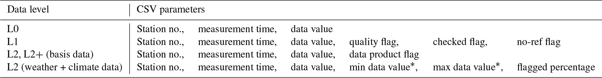
^* Temporal minimum and maximum values; only available for temperature, soil moisture (derived from pF value), and wind peak gust data.

Data are available both as time series in CSV format (see Table 7 for a description of the CSV format) and, for L2 and L2+ only, as gridded data in NetCDF format (see Tables A3 and A4 for a list of variables available in the NetCDF files).

5.1 Level 0 data and level 1 data

L0 data are raw data values written into the database by the CRAS as described in Sect. 4.1. They are available for expert users only. A download option is offered as CSV files via the data portal.

L1 data are quality-controlled L0 values containing the data and associated flags (see Sect. 4.2).

5.2 Level 2 and 2+ data

L2 data are available both as time series data in CSV format (all variables) and as gridded data in NetCDF format (main parameters, i.e., air temperature, relative humidity, and precipitation only). See Sect. 4.3 and 4.5 for information on the L2 data generation.

L2+ data are either time series (in case of soil moisture data) or gridded data (in case of heat index and wind data), derived from basic level 2 data and auxiliary data or models by using functional dependencies or modeling (see also Sect. 4.4).

The L2 and L2+ time series data can be plotted in the data portal and downloaded as CSV files. The data are available in basis data resolution (5 min for WegenerNet FBR and 10 min for WegenerNet JBT) and time-aggregated as half-hourly, hourly, daily, monthly, seasonal, and annual data.

Level 2 and 2+ gridded data products are available in NetCDF format. See Table A3 for a list of all parameters stored in the NetCDF files. The data are available in a base temporal resolution of 5 min for WegenerNet FBR and 10 min for WegenerNet JBT and time-aggregated as half-hourly, hourly, daily, monthly, seasonal, and annual data. The spatial resolution of the grids is 200 m × 200 m.

Gridded wind field data products are available in NetCDF format and can be downloaded via the data portal. See Table A4 for a list of all parameters stored in the wind NetCDF files. The data are available in a base temporal resolution of 30 min and time-aggregated as hourly, daily, monthly, seasonal, and annual data. The spatial resolution of the grids is 100 m × 100 m.

5.3 Auxiliary data

In addition to the meteorological data described above, a growing number of auxiliary data are available for the WegenerNet and can be downloaded via the data portal. These data currently include a digital elevation model (DEM), land use–land cover data, and hydro-pedological soil characteristics, all provided by state offices of the regional government of Styria, Austria.

The DEM is available at a horizontal resolution of 10 and 100 m for both the WegenerNet FBR and WegenerNet JBT and also at 200 m resolution for the WegenerNet FBR. The data originate from the geographic information system (GIS) server of the government of Styria (http://gis.steiermark.at, last access: 14 May 2019).

Land use–land cover data are available at a horizontal resolution of 100 m and cover the WegenerNet FBR and its surroundings. They originate from a project to classify the hydro-pedological characteristics of the Raab valley and southeastern Styria (Klebinder et al., 2017). Additional data from this project are available, but due to copyright reasons they must be requested from the WEGC. They include soil type (content of silt, clay, and sand), saturated hydraulic conductivity k_sat, total pore volume, air capacity, permanent wilting point, available water capacity, the Mualem–van Genuchten parameters (θ_r, θ_s, α, and n), runoff coefficients, and soil moisture distribution.

6 Example applications

We decided to show just two “arbitrary” examples for illustration out of the many possible uses of the WegenerNet dataset. Section 6.1 presents a multi-variable view of meteorological data for a storm event caused by a midlatitude cyclone in 2017, and Sect. 6.2 presents high-resolution gridded precipitation and temperature data for a strong convective event. We note that the WegenerNet data, including predecessors of the version 7.1 dataset, have been applied in a wide variety of scientific uses so far, such as the studies summarized in Sect. 2 above.

6.1 Storm event due to midlatitude Cyclone Xaver

6.1.1 Multi-variable time series

Figure 3 shows meteorological data before and during the passage of midlatitude Cyclone Xaver (3 March 2017, 00:00:00 UTC–5 March 2017, 06:00:00 UTC) at four different WegenerNet stations: two in the WegenerNet FBR (no. 44, located atop a silo in the Raab valley at 55 m above ground, and no. 77, located in the center of the region at 10 m above ground) and two on the WegenerNet JBT (no. 501, Oberkainz, on the Johnsbach valley floor, at 930 m m.s.l. (located 10 m above ground), and no. 505 at the peak of Mount Zinödl, at 2197 m m.s.l. (located 6 m above ground)). The cyclone formed over the Bay of Biscay on 3 March 2017, moving northwards and then crossing Ireland on 4 March 2017. On the same day, a trough was formed, reaching down to the eastern end of the Pyrenees. The Alps were lying between this trough and a strong anticyclone (named Hertha) with its center over the Black Sea. As a consequence, a strong föhn storm occurred over the Alps. On 5 March 2017, Xaver crossed Scotland in a northeasterly direction and then moved further north, losing its influence on the Central European weather (Janke, 2017; Deutscher Wetterdienst and FU-Berlin/BWK, 2017a, b, c).

Figure 3 Level 2 time series data of meteorological conditions before and during the passage of midlatitude Cyclone Xaver on 3–5 March 2017 at four different WegenerNet stations – two in the Feldbach region (44 and 77) and two in the Johnsbachtal region (501 and 505).

As shown in Fig. 3, peak wind gust velocities at station 505 reached a maximum of 46.0 m s⁻¹ on 4 March 2017, at 18:40:00 UTC, blowing from a southerly direction. The maximum 10 min average wind velocity was reached a bit earlier, at 17:50:00 UTC, with 28.6 m s⁻¹, coinciding with a sharp rise in temperature of 7 ^∘C between 17:30:00 UTC and 18:10:00 UTC. On the Johnsbach valley floor (station 501), maximum wind speed and peak gust velocities were reached much earlier, at 08:30:00 UTC on the same day, with velocities of 8.5 and 18.9 m s⁻¹, respectively.

In the WegenerNet FBR, average wind and peak gust velocities reached their maximum values around 12:00:00 UTC, with 12.4 and 18.3 m s⁻¹, respectively.

6.1.2 Gridded wind gust speed data

Figure 4 shows gridded wind gust speed data for the above-mentioned föhn storm as generated by the WPG, with Fig. 4a showing the situation pre-onset, with gusts up to about 15 m s⁻¹, and Fig. 4b showing the maximum of the storm, with gusts up to about 49 m s⁻¹. In both plots, the structure of the mountainous terrain is clearly visible, with increasing wind speeds at higher altitudes.

6.2 Precipitation and temperature data of a heavy local-scale thunderstorm

Figure 5 shows gridded 5 min precipitation sums (left) and temperature data (right) of a heavy local thunderstorm moving from north to south through the western part of the Feldbach region on 7 July 2017. Three snapshots are shown.

At 13:25:00–13:30:00 UTC, the cell was located slightly south of the Raab valley. While temperatures in the southeastern part of the region still reached about 30 ^∘C, they were already much cooler (about 18 ^∘C) in the vicinity of the storm. At 13:35:00–13:40:00 UTC, the cell moved further south, and at 13:40:00–13:45:00 UTC, precipitation intensity peaked, with a 5 min precipitation sum of 19.5 mm at station 142. The associated temperature data in Fig. 5d–f show a drop of about 10 ^∘C as the storm moved through the region.

Figure 4 Modeled wind gust fields for the WegenerNet Johnsbachtal area before and during the passage of midlatitude Cyclone Xaver. (a) Pre-onset on 3 March 2017 at 06:00:00–06:30:00 UTC and (b) at its maximum on 4 March 2017 at 16:00:00–16:30:00 UTC.

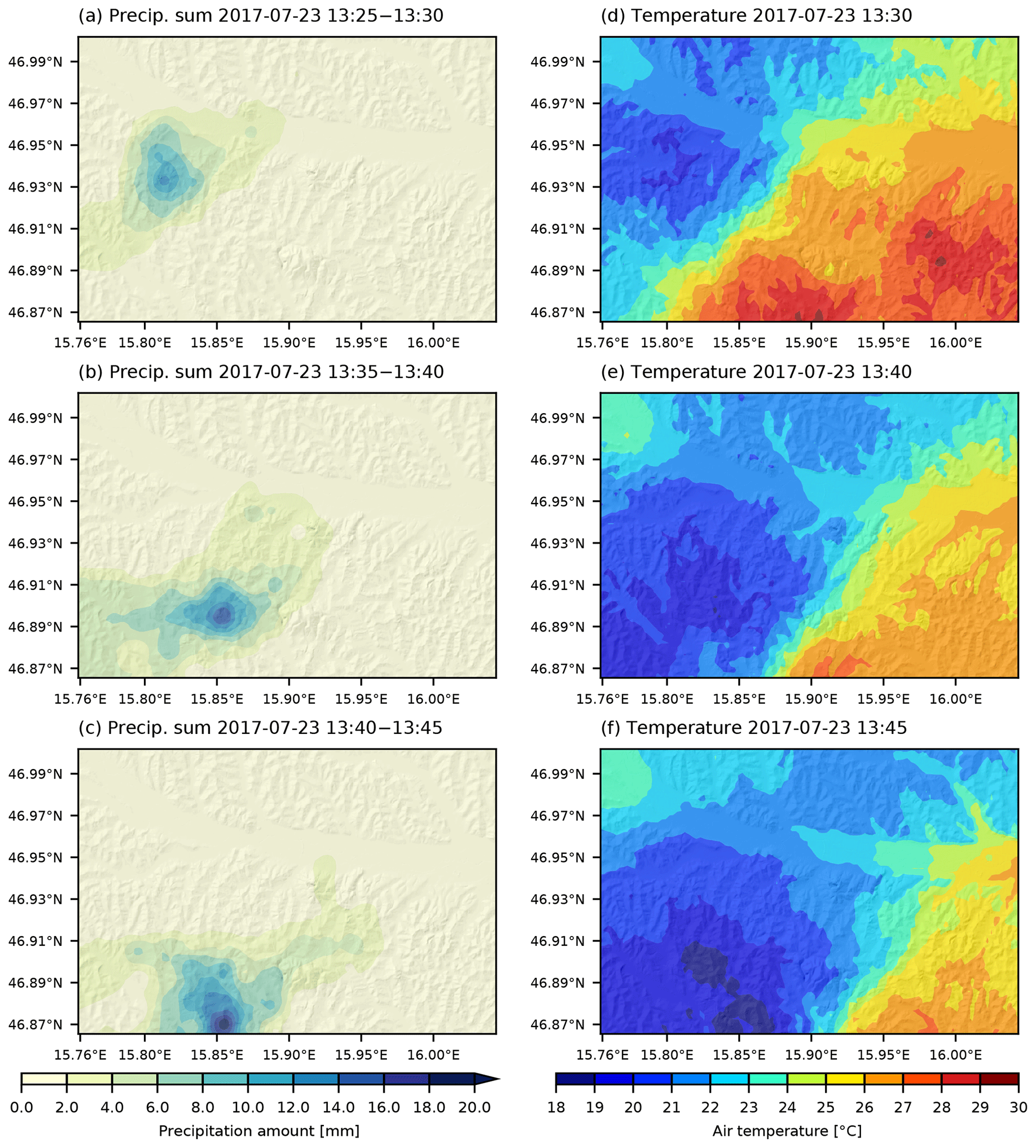
Figure 5 Gridded fields of 5 min precipitation sums (a, b, c) of a strong local-scale thunderstorm cell moving through the western part of the WegenerNet Feldbach Region and associated temperature field data (d, e, f).

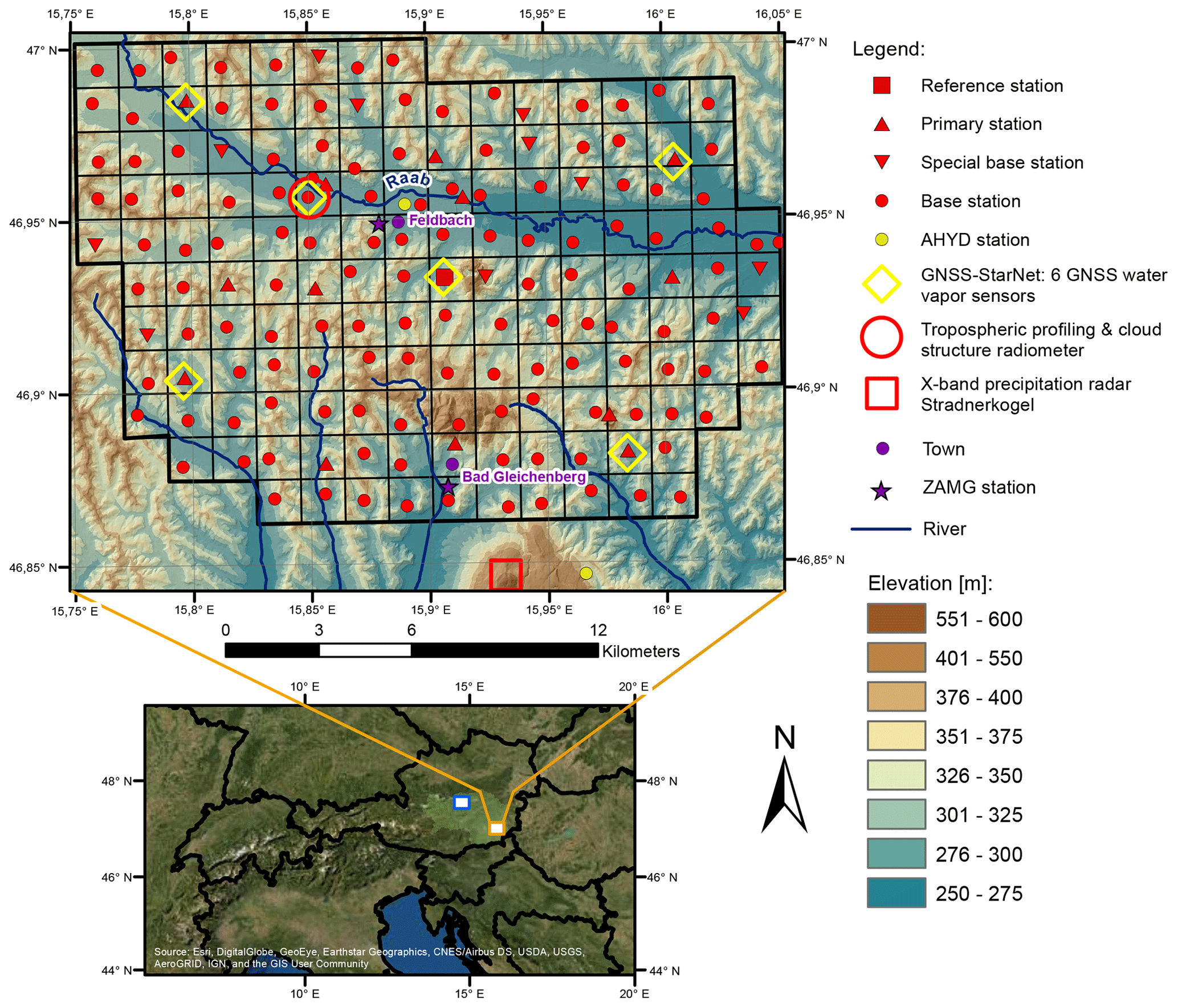
Figure 6 The WegenerNet Feldbach Region (FBR) 3D Open-Air Laboratory for Climate Change Research, consisting of the ground station network as described in this paper and additional 3D-observing-system components including an X-band precipitation radar; a tropospheric profiling and cloud structure radiometer pair; and a GNSS station network called GNSS-StarNet, comprising six GNSS receivers for water vapor sensing. The legend on the right explains all map characteristics.

7 Outlook

In 2020, the WegenerNet FBR network was upgraded with three new major observing components, expanding it from a 2D ground station hydrometeorological network into a 3D open-air laboratory for climate change research at very high resolution.

The following new atmospheric 3D-observation components, as shown in the most recent WegenerNet FBR instrumentation map in Fig. 6, started operations in 2020.

1. A polarimetric X-band Doppler weather radar for studying precipitation parameters in the troposphere above the ground network, such as rain rate, hydrometeor classification, Doppler velocity, and approximate drop size distribution and number: it can provide 3D volume data (at about 1 km × 1 km horizontal and 500 m vertical resolution and 2.5 min time sampling) for moderate to strong precipitation. Together with the dense ground network, this allows detailed studies of heavy precipitation events at high resolution and accuracy.

2. A radiometer pair consisting of two azimuth- and elevation-steerable radiometers: (1) a microwave atmospheric-profiling radiometer with built-in auxiliary infrared radiometer for vertical profiling of temperature, humidity, and cloud liquid water in the troposphere above the WegenerNet area (with about 100 m to 1 km vertical resolution and 5 to 10 min time sampling), also capable of measuring cloud-base heights, vertically integrated water vapor (IWV), and slant IWV along line-of-sight paths towards Global Navigation Satellite System (GNSS) satellites, and (2) a complementary infrared cloud structure radiometer at similar spatiotemporal sampling for further refining gridded cloud-base height calculations and enabling multi-layer cloud-field reconstruction over the WegenerNet area, providing 3D cloud-field (multi-layered cloud fraction) estimates.

3. A water-vapor-mapping high-resolution GNSS station network named GNSS-StarNet, comprising six ground stations and spatially forming two star-shaped subnets across the WegenerNet area (one with ∼ 10 km interstation distance and one embedded with ∼ 5 km interstation distance), for providing slant IWV, vertical IWV, and precipitable water, among other parameters, at 2.5 to 15 min time sampling.

The WegenerNet JBT network will be expanded with a new station in the Enns valley, measuring air temperature, humidity, precipitation, radiation, snow height, and wind. This will allow more accurate wind modeling in the WegenerNet JBT area in particular following a recommendation by Schlager et al. (2018, 2019) based on their JBT wind field quality evaluations.

Data from these new components will be made available via the WegenerNet data portal, and a description of the components is planned for a future paper.

Regarding improvements to the processing system, a version of the QCS which is capable of processing daily time periods (in contrast to 3-hourly time periods in the current version) is presently being developed in the course of a master's thesis. This will lead to improvements in the quality of precipitation data for cases like blocked gauges or melting snow, where the QCS algorithms gain additional information from the larger sample size.

Another future improvement will be the implementation of a new algorithm for the calculation of temperature lapse rates in the DPG (see also step 3 of Sect. 4.3), which was developed in the course of a master's thesis (Hocking, 2020).

8 Data availability

The data described in this article are published at https://doi.org/10.25364/WEGC/WPS7.1:2021.1 (Fuchsberger et al., 2021). This DOI contains data from version 7.1 of the WegenerNet Processing System for the period 1 January 2007 to 31 December 2020. New data under this version beyond 2020 are continuously added to the database and are available via the WegenerNet data portal at http://www.wegenernet.org (last access: 20 January 2021). For reasons of consistency, new data DOIs are generated on a regular basis (at least once per year), expanding the time range documented in this paper. The DOIs will be made available on the data portal's entry page upon release and can be used together with this paper to properly cite the WegenerNet dataset.

9 Conclusions

This paper provides an overview of the current state of the WegenerNet climate station networks Feldbach Region (FBR) and Johnsbachtal (JBT), their processing system, and their data products. It is the first major update to a WegenerNet introduction and overview paper published in the Bulletin of the American Meteorological Society (BAMS) in 2014 (Kirchengast et al., 2014), and it is hence foreseen to serve as the newest up-to-date reference for all WegenerNet data users of the currently implemented data version 7.1.

Appendix A

Table A1 Sensors installed in the WegenerNet FBR (alphabetical order by parameter); installed data loggers are stated in the table's bottom row.

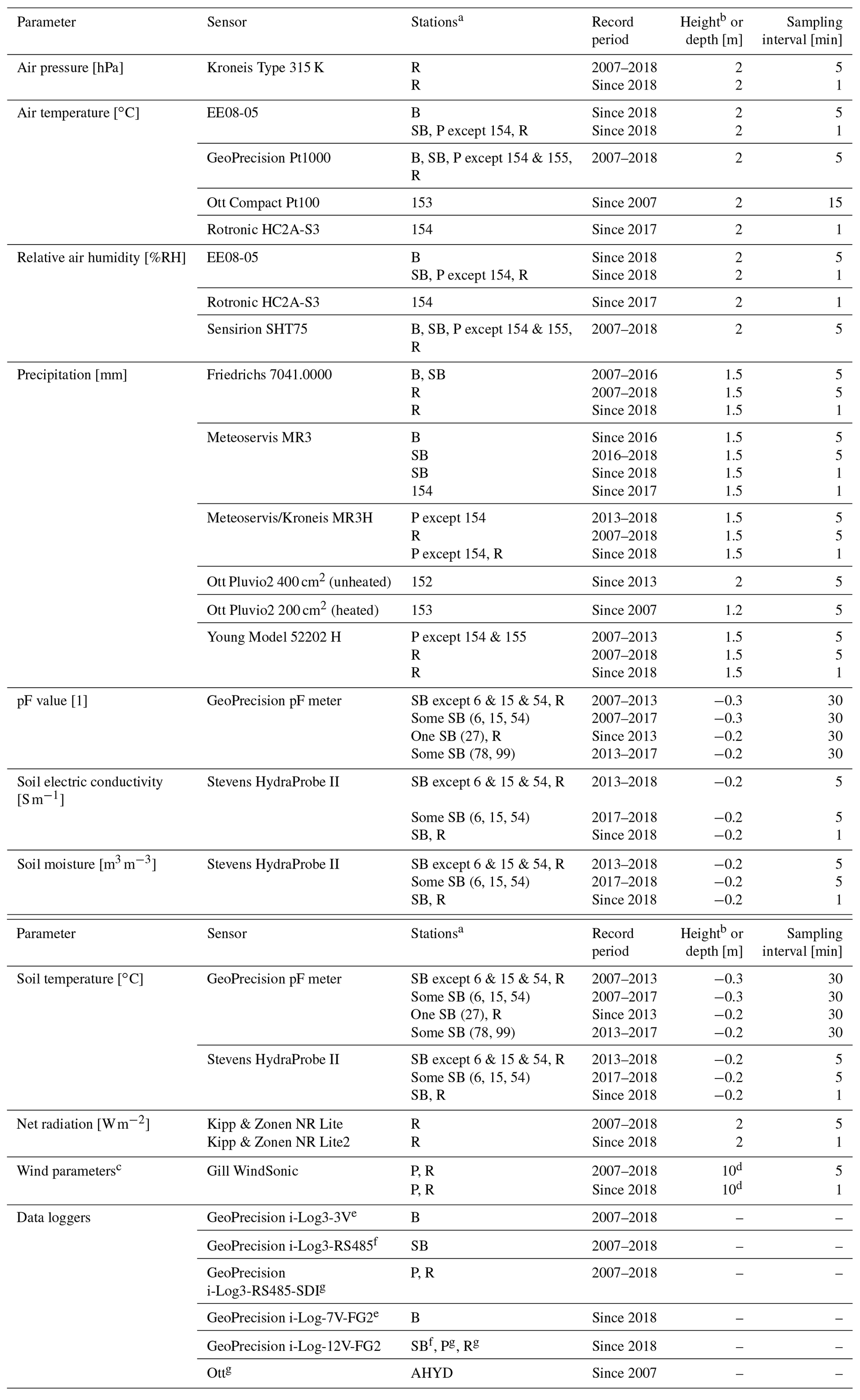
^a Station types comprise B: base stations; SB: special base stations; P: primary stations; R: reference station; and AHYD: stations operated by the Austrian Hydrographic Service; see also Table 1. ^b For denoted stations, except station 44 (a silo rooftop station in the Raab valley), which measures temperature and relative humidity at a height of 53 m, precipitation at 51 m, and wind parameters at 55 m. ^c Wind parameters comprise speed [m s⁻¹], direction [^∘], gust speed [m s⁻¹], and gust direction [^∘]. ^d Height for stations 44, 72, and 101 is 55, 18, and 14 m, respectively. ^e Battery-powered. ^f Powered by solar panel and battery. ^g Grid-powered with backup battery.

Table A2 Sensors installed in the WegenerNet JBT (alphabetical order by parameter); installed data loggers are stated in the Table's bottom row.

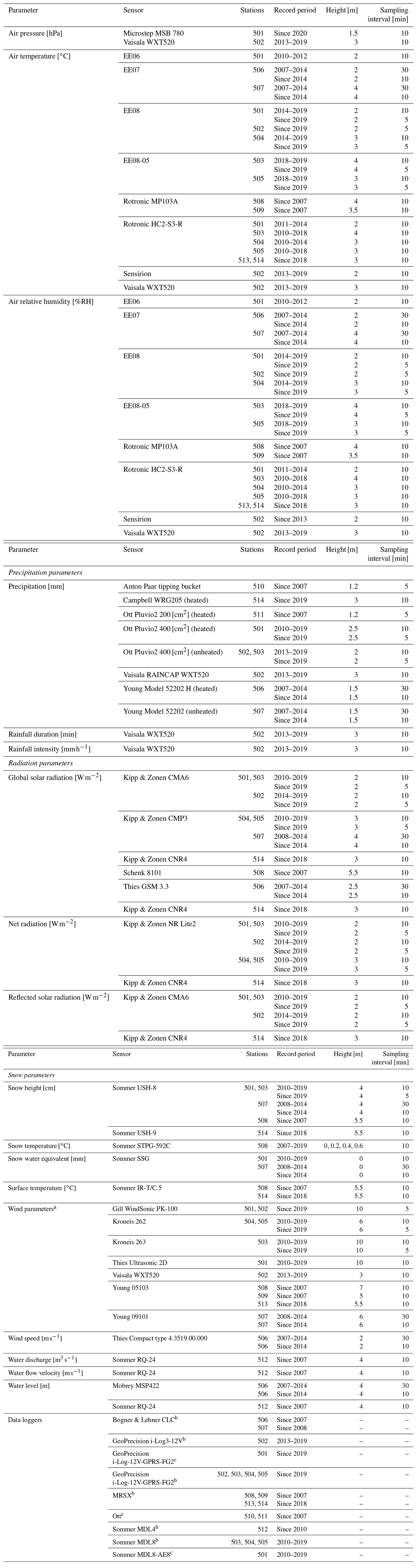
^a Wind parameters comprise speed [m s⁻¹], direction [^∘], gust speed [m s⁻¹], and gust direction [^∘]. ^b Powered by solar panel and battery. ^c Grid-powered with backup battery.

Table A3 List of variables of WegenerNet level 2 and 2+ NetCDF data.

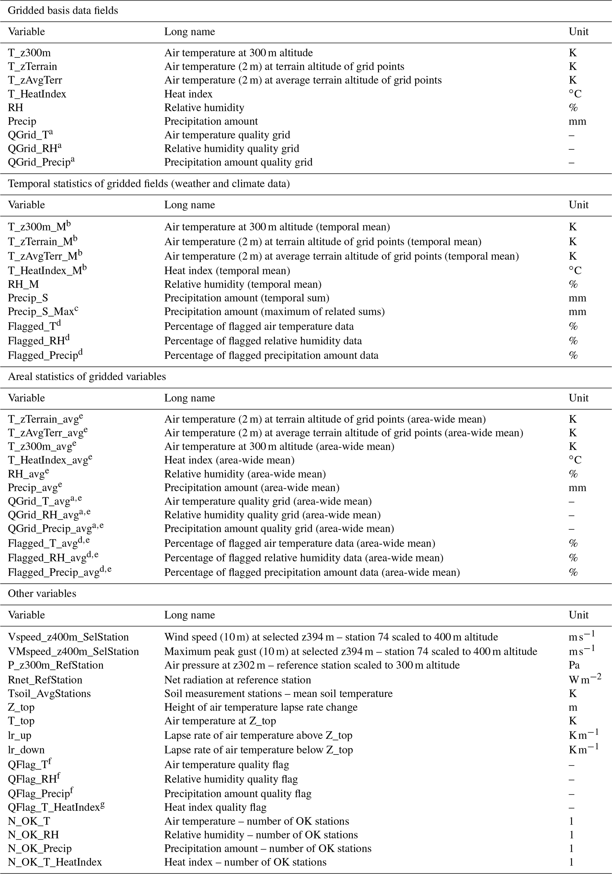
^a Refers to the interpolated DP-Flag grids as described in Sect. 4.3, point 4. ^b Given variables are also available as temporal maximum and minimum, indicated by variable name extension _Max, and _Min. ^c Available for climate data only. ^d Refers to the flagged percentage of data grids as described in Sect. 4.5.2. ^e Given variables are available as area-wide mean, maximum, minimum, and standard deviation, indicated by variable name extensions _avg, _max, _min, and _sdev. ^f Same as QGrid_[T,RH,Precip]_avg, available for compatibility reasons only. ^g Average of QFlag_T and QFlag_RH.

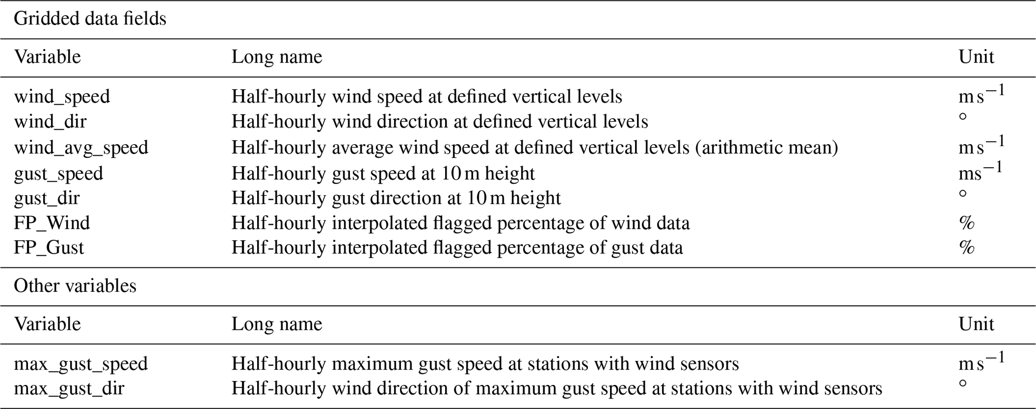
Table A4 List of variables of WegenerNet wind field NetCDF data.

Appendix B: Abbreviations

The following abbreviations are used in this paper:

AHYD	Austrian Hydrographic Service
BAMS	Bulletin of the American Meteorological Society
CALMET	California Meteorological Model
CRAS	Command Receive Archiving System
CSV	Comma-separated values
DEM	Digital elevation model
DP-Flag	Data product flag
DPG	Data Product Generator
DWD	Deutscher Wetterdienst
FBR	Feldbach Region
FP	Flagged percentage of data
GIS	Geographic information system
GNSS	Global navigation satellite system
IDSW	Inverse-distance-squared weighting
IDW	Inverse distance weighting
IGR	Institute of Geography and Regional Science
IWV	Integrated water vapor
JBT	Johnsbachtal
L0	Level 0 (data)
L1	Level 1 (data)
L2	Level 2 (data)
m.s.l.	Above mean sea level
NaN	Not a number
NPG	National Park Gesäuse
ÖBB	Österreichische Bundesbahnen (Austrian Federal Railways)
QCS	Quality Control System
QF	Quality flag
VAPG	Value-Added Product Generator
WCPG	Weather and Climate Products Generator
WEGC	Wegener Center for Climate and Global Change
WMITS	WegenerNet Monitoring and Issue Tracking System
WPG	Wind Product Generator
WPS	WegenerNet Processing System
ZAMG	Zentralanstalt für Meteorologie und Geodynamik (Central Institute for Meteorology and Geodynamics; Austrian national weather service)
ZAWS	ZAMG avalanche warning service