the Creative Commons Attribution 4.0 License.
the Creative Commons Attribution 4.0 License.
 | 05 Mar 2020
Geometric accuracy assessment of coarse-resolution satellite datasets: a study based on AVHRR GAC data at the sub-pixel level
Kathrin Naegeli
Stefan Wunderle
AVHRR Global Area Coverage (GAC) data provide daily global coverage of the Earth, which are widely used for global environmental and climate studies. However, their geolocation accuracy has not been comprehensively evaluated due to the difficulty caused by onboard resampling and the resulting coarse resolution, which hampers their usefulness in various applications. In this study, a correlation-based patch matching method (CPMM) was proposed to characterize and quantify the geo-location accuracy at the sub-pixel level for satellite data with coarse resolution, such as the AVHRR GAC dataset. This method is neither limited to landmarks nor suffers from errors caused by false detection due to the effect of mixed pixels caused by a coarse spatial resolution, and it thus enables a more robust and comprehensive geometric assessment than existing approaches. Data of NOAA-17, MetOp-A and MetOp-B satellites were selected to test the geocoding accuracy. The three satellites predominately present west shifts in the across-track direction, with average values of −1.69, −1.9, −2.56 km and standard deviations of 1.32, 1.1, 2.19 km for NOAA-17, MetOp-A, and MetOp-B, respectively. The large shifts and uncertainties are partly induced by the larger satellite zenith angles (SatZs) and partly due to the terrain effect, which is related to SatZ and becomes apparent in the case of large SatZs. It is thus suggested that GAC data with SatZs less than 40∘ should be preferred in applications. The along-track geolocation accuracy is clearly improved compared to the across-track direction, with average shifts of −0.7, −0.02 and 0.96 km and standard deviations of 1.01, 0.79 and 1.70 km for NOAA-17, MetOp-A and MetOp-B, respectively. The data can be accessed from https://doi.org/10.5676/DWD/ESA_Cloud_cci/AVHRR-AM/V002 (Stengel et al., 2017) and https://doi.org/10.5067/MODIS/MOD13A1.006 (Didan, 2015).
- Article
(2954 KB) - Full-text XML
- BibTeX
- EndNote


Advanced Very High Resolution Radiometer (AVHRR) data provide valuable data sources with a near-daily global coverage to support a broad range of environmental monitoring research, including weather forecasting, climate change, ocean dynamics, atmospheric soundings, land cover monitoring, search and rescue, forest fire detection, and many other applications (Van et al., 2008). The unique advantage of AVHRR sensors is their long history dating back to the 1980s and thus enabling long-term analyses at climate-relevant timescales that cannot be covered by other satellites. However, AVHRR data are rarely used at the full spatial resolution for global monitoring due to the limited data availability (Pouliot et al., 2009; Fontana et al., 2009). Instead, the Global Area Coverage (GAC) AVHRR dataset with a reduced spatial resolution is generally employed in long-term studies at a global or regional perspective (Hori et al., 2017; Delbart et al., 2006; Stöckli and Vidale, 2004; Moulin et al., 1997).
However, there are several known problems with the geo-location of AVHRR GAC data, which have a profound impact on their application. (1) The drift of the spacecraft clock results in errors in the along-track direction (Devasthale et al., 2016). Generally, an uncertainty of 1 s approximately induces an error of 8 km in this direction. (2) Satellite orientation and position uncertainties influence the projection of the satellite geometry to the ground, which leads to errors in both along-track and across-track directions. (3) Earth surface elevation aggravates distortions in the across-track direction (Fontana et al., 2009). Without navigation corrections, the spatial misplacement of the GAC scene caused by these factors can be up to 25–30 km occasionally (Devasthale et al., 2016).
For geocoding of AVHRR data, a two-step approach is usually used: (1) geocoding based on orbit model, ephemeris data and time of onboard clock (Van et al., 2008), achieving an accuracy within 3–5 km depending on the accuracy of orbit parameters and model (Khlopenkov et al., 2010), and (2) using any kind of ground control points (GCPs) (e.g., road or river intersections, coastal lines) to improve geocoding (Takagi, 2004; Van et al., 2008). Additionally, in order to eliminate the ortho-shift caused by elevations, an orthorectification would be needed (Aguilar et al., 2013; Khlopenkov et al., 2010). The dataset used in this study is from the ESA (European Space Agency) cloud CCI (Climate Change Initiative) project, which has corrected clock drift errors by coregistration of AVHRR GAC data with a reference dataset and showed improved navigation by fitting the data to coastal lines.
Unlike the Local Area Coverage (LAC) data with a full spatial resolution of AVHRR, GAC data are sampled on board the satellite in real time to generate coarser-resolution data (Kidwell, 1998). This is achieved by averaging values from four out of five pixel samples along a scan line and eliminating two out of three scan lines, resulting in a spatial resolution of 1.1 km×4 km along the scan line with a 3 km distance between pixels across the scan line. Therefore, the nominal size of a GAC pixel is 3 km×4.4 km. It is important to note that the spatial resolution of GAC data also depends on the satellite zenith angle (SatZ). Because of the large swath width, the spatial resolution of LAC decreases to 2.4 km by 6.9 km at the edge of the swath (D'Souza and Malingreau, 1994). With the selection process for GAC, the GAC resolution is also much worse than 4 km. Furthermore, the onboard resampling process of GAC data makes the orthorectification not feasible, which results in lowering of geolocation accuracy in the across-track direction. The final quality of AVHRR GAC data has not been quantified and we, therefore, make an attempt to assess their geolocation accuracy, particularly over terrain areas.
There are generally three approaches to assess the non-systematic geometric errors of satellite images: (1) the coastline crossing method (CCM) which detects the coastline in the along-track and across-track directions through a cubic polynomial fitting (Hoffman et al., 1987); (2) the land–sea fraction method (LFM) which develops a linear radiance model as a function of land–sea fraction and land and sea radiance and then finds the minimum difference between model-simulated and instrument-observed radiance by shifting the pixels in the along-track and across-track directions (Bennartz, 1999); and (3) the coregistration method which computes the difference or similarity relative to a reference image (Khlopenkov et al., 2010). The abilities of these three methods in characterizing the geometric errors are limited and dependent on different, method-dependent factors. The CCM is subject to the structure of the coastline, and the LFM depends on the accuracy of the land–sea model but shows advantages on complex coastlines (Han et al., 2016). The coregistration method is usually applied to high-resolution visible and infrared images (Wang et al., 2013; Wolfe et al., 2013) as it relies on individual objects/landmarks in both datasets. However, when it comes to coarse-resolution data with several kilometers' pixel size, the main difficulties arise from false detection due to the effect of mixed pixels, which hampers the application of the existing methods. An approach assessing the geolocation accuracy of coarse-resolution satellite data is thus strongly needed. The geometric accuracy is important as even small geometric errors can lead to significant noises on the retrieval of surface parameters, such as normalized difference vegetation index (NDVI), leaf area index (LAI) and albedo, which mask the reality or bias the final results and conclusions (Khlopenkov et al., 2010; Arnold et al., 2010). For instance, anomalous NDVI dynamics during the regeneration phase of forest-fire-burnt areas can be explained by the imprecise geolocation of the dataset used (Alcaraz-Segura et al., 2010). Therefore, it is critical to develop a rigorous geometric accuracy assessment method in order to ensure the effectiveness of AVHRR GAC data in the generation of climate data records (CDRs) (Khlopenkov et al., 2010; Van et al., 2008).
Based on the idea of the coregistration method, this study proposes a method named correlation-based patch matching method (CPMM), which is capable of quantifying the geometric accuracy of coarse-resolution satellite data available as fundamental climate data records (FCDRs) for global applications (Hollmann et al., 2013). We show the procedure based on AVHRR GAC data, which are compiled for the ESA CCI cloud project (Stengel et al., 2017) and are now also used for the ESA CCI+ snow project. The assessment is conducted at the sub-pixel level and not affected by the mixed pixel problem. This method is tested using satellite data from NOAA-17, MetOp-A and MetOp-B, respectively. Furthermore, the potential factors that cause geometric distortions are explored and discussed. Although the band-to-band registration (BBR) accuracy assessment is an important aspect for such multi-spectral images, it is not a focus of this study, since the BBR accuracy of AVHRR has been comprehensively evaluated by a previous study (Aksakal et al., 2015).
2.1 Satellite data
AVHRR is a multipurpose imaging instrument aboard the NOAA satellite series since 1978 and the Meteorological Operational Satellites (MetOp) operated by EUMETSAT since 2006, delivering daily information of the Earth in the visible, near-infrared and thermal wavelengths. They provide observations from four to six spectral bands, depending on the generation of AVHRR sensors. This study only focuses on the AVHRR GAC data observed by NOAA-17 (AVHRR-3 generation), MetOp-A and MetOp-B. The spectral characteristics of the AVHRR sensors on board these three platforms are the same and summarized in Table 1. Since the spatial resolution of AVHRR GAC data is often considered to be 4 km (Fontana et al., 2009), the analysis in this study was conducted at the 4 km level using the data acquired on 13 August 2003 for NOAA-17 and 12 March 2017 for MetOp-A and MetOp-B.
Table 1Spectral characteristics of AVHRR sensors.
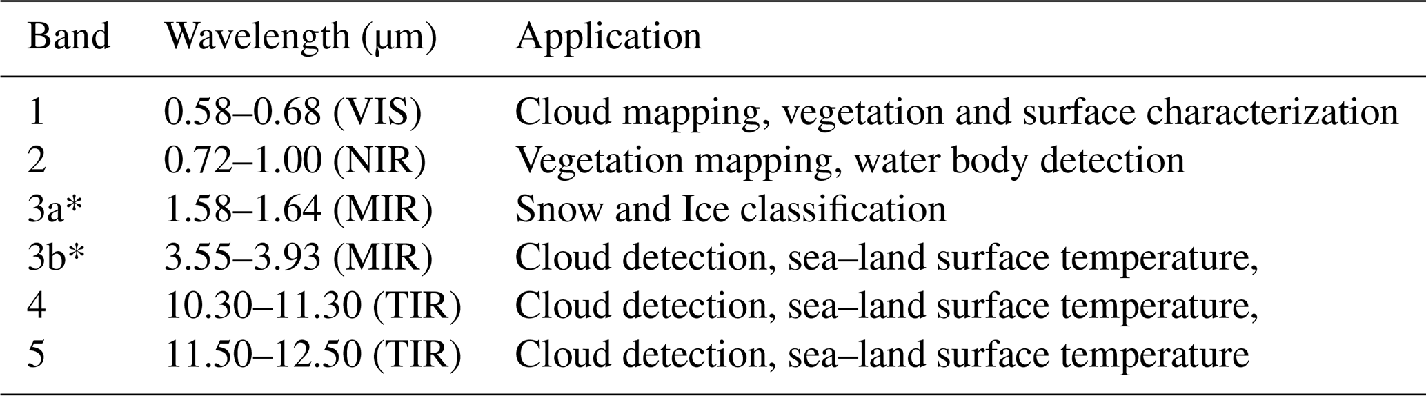
* Note the channel 3a is only used continuously on NOAA-17 and MetOp-A. Onboard MetOp-B channel 3a was only active during a limited time span.
From a standpoint of geometric accuracy assessment, the reflectances in bands 1 and 2 were employed in this study. However, these two bands are not only affected by the atmosphere but also by the earth surface anisotropy characterized by the bidirectional reflectance distribution function (BRDF) (Cihlar et al., 2004). Given the fact that BRDF effects can be reduced through the calculation of vegetation indices such as NDVI (Lee and Kaufman, 1986), the NDVI is employed in this study, which is derived from the reflectance in bands 1 and 2 according to Eq. (1).
where R1 and R2 refer to the reflectance in bands 1 and 2, respectively. It is important to note that during the process of generating NDVI, the atmospheric and BRDF corrections were not performed. But it is expected that such effects originating from these omissions are of minor influence, because the method of this study is based on correlation analysis and does not rely on absolute values of NDVI. Another advantage of using NDVI is that it has higher contrast between different land cover types, such as vegetation and no-vegetation, snow and no-snow, etc. Furthermore, in order to investigate the effect of off-nadir viewing angle on geometric accuracy, the SatZ data of AVHRR were also extracted.
Ideally, the referenced data in geometric quality assessment should meet the required accuracy of a one-third field of view (FOV) (WMO and UNEP, 2006) and also satisfy the accuracy requirement of an order of magnitude better than 1∕10 of the image spatial resolution (Aksakal, 2013), which means 400 m for the AVHRR GAC data. The NDVI provided by the MOD13A1 V006 product was introduced as a source of reference data to perform the geometric quality assessment, because the sub-pixel accuracy of the MODIS product is sufficient to satisfy this requirement (Wolfe et al., 2002). The high geolocation accuracy of MODIS products was achieved by using the most advanced data processing system, which has updated the models of spacecraft and instrument orientation several times since launch. Consequently, the various geolocation biases resulting from instrument effects and sensor orientation are removed (Wolfe et al., 2002). The NDVI data with the date corresponding to that of AVHRR GAC data were obtained from the Level-1 and Atmosphere Archive and Distribution System (LAADS) Distributed Active Archive Center (DAAC) (https://ladsweb.modaps.eosdis.nasa.gov/, last access: 17 November 2018) with the sinusoidal projection at a spatial resolution of 500 m and a temporal resolution of 16 d. The detailed description of the MOD13A1 V006 product can be found in Didan (2015).
2.2 Geographical regions of interest
The purpose of this study is not only to assess the geolocation accuracy of 4 km AVHRR GAC data, but also to explore the potential impact factors related to geolocation accuracy. Therefore, the investigations were made at different latitudes and longitudes, at different locations with different SatZs, for different land covers, as well as different topographies. The swaths covering parts of Europe (including the Alps) and Africa were used since they fit the study needs (Fig. 1). Investigations were based on six regions of interest (ROI) as shown in Figs. 1 and 2. The ROIs from 1 to 6 enable us to investigate the geolocation accuracy at different SatZs, topography, as well as latitudes and longitudes. Their locations and extents are consistent for the scenes from NOAA-17 and MetOp-A (Fig. 1), which enables the comparison of geolocation accuracy between these two sensors. The size of ROI was set as large as possible in order to get more significant and comprehensive results. On the other hand, areas covered by cloud and water have to be avoided, resulting in the different sizes of these ROIs. Half of the ROIs (ROIs 2, 4, 6) serve as a good example for a typical mountainous area on Earth. The other half of ROIs (ROIs 1, 3, 5), on the other hand, mainly cover relatively flat areas. Since the NOAA-17 scene was almost unaffected by cloud, another ROI (ROI 7) was selected to check the geolocation accuracy at nadir. The MetOp-B scene was influenced by cloud but served as a good example to illustrate the combined effect of topography and large SatZs (Fig. 2). Although there are also six ROIs (ROIs (a–f)) selected, their sizes and extents are totally different from the above two scenes. In order to include the terrain area, two subsets were used (Fig. 2a and c). Each grid in the ROI represents the minimum unit (namely the patch) based on which we conduct the geometric quality analysis.
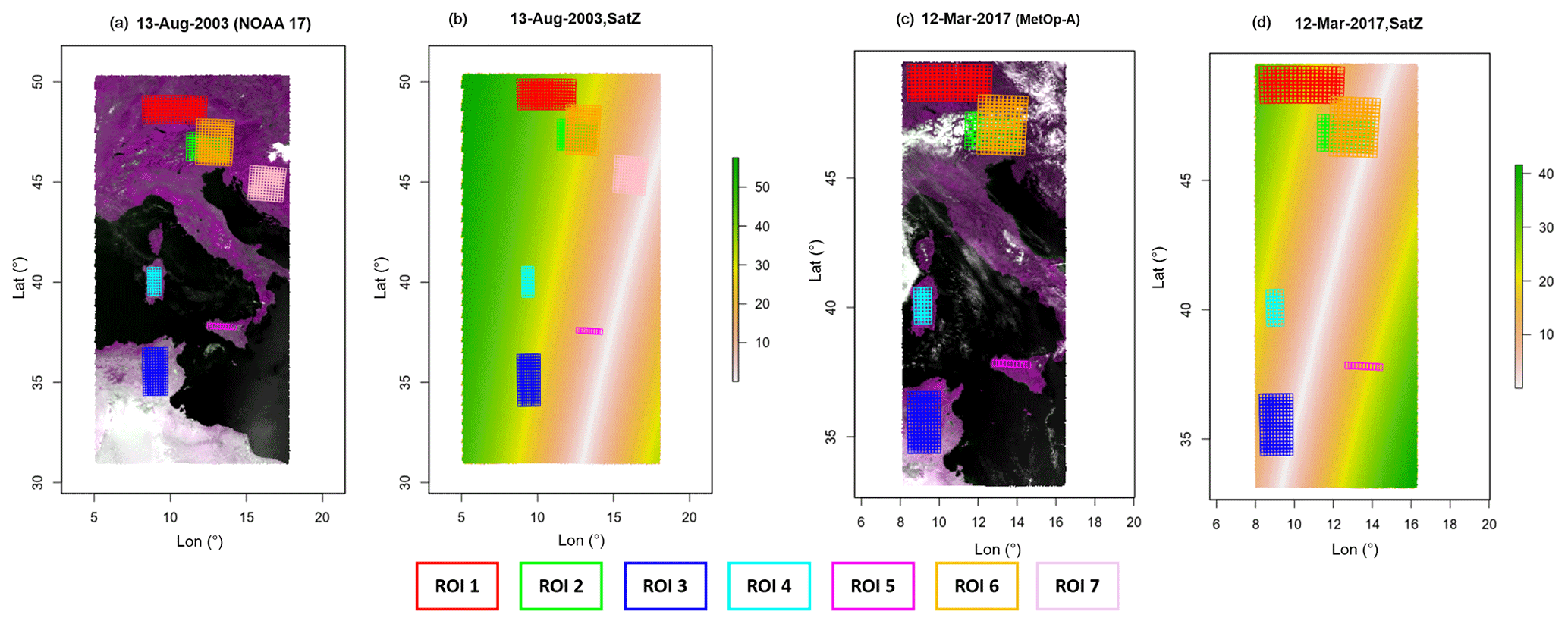
Figure 1Top-of-atmosphere reflectance true color composite (AVHRR GAC bands 2-1-2) surrounding the study area (a, c) and the distribution of ROIs (as defined by rectangles with different colors) over the study area. Panels (a) and (c) are the data from NOAA-17 and MetOp-A satellites on 13 August 2003 and 12 March 2017, respectively. Panels (b) and (d) are their corresponding SatZs, respectively, which is indicated by the color bar, with the white line representing small SatZs along the satellite path. These data are available from the ESA CCI (Climate Change Initiative) cloud project (Stengel et al., 2017).
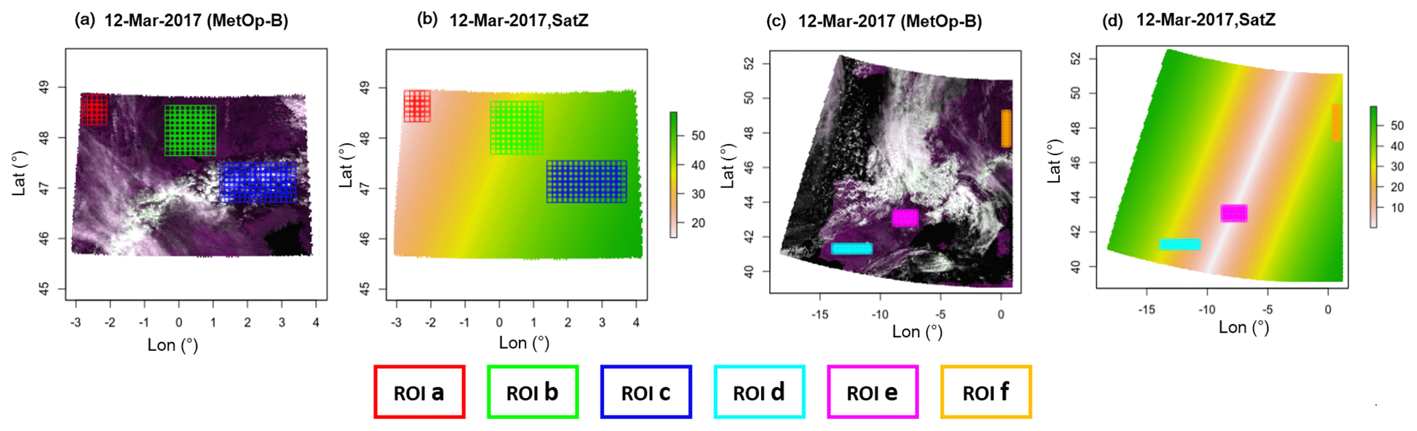
Figure 2Top-of-atmosphere reflectance true color composite (AVHRR GAC bands 2-1-2) from the MetOp-B satellite on 12 March 2017 (a, c) and the distribution of ROIs (as defined by rectangles with different colors) over the study area. Panels (a) and (c) indicate the two subsets of the dataset corresponding to different areas. Panels (b) and (d) are their corresponding SatZs (indicated by the color bar), respectively. The white line in (d) represents small SatZs along the satellite path. These data are available from the ESA CCI (Climate Change Initiative) cloud project (Stengel et al., 2017).
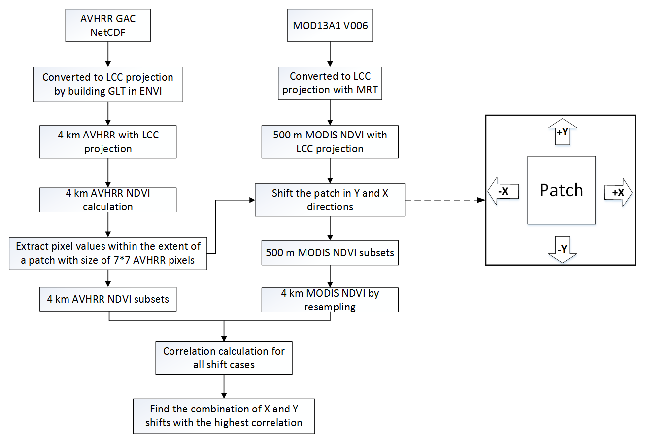
The assessment was performed by comparing the AVHRR GAC scenes with geo-located reference data, i.e., MOD13A1 (V006). An approach named the correlation-based patch matching method (CPMM) is proposed to find the best match between small image patches taken from the reference images and the AVHRR GAC images. This method is expected to be more suitable for the geometric accuracy assessment of coarse-resolution images than the current methods, i.e., the CCM, LFM and co-registration using shorelines. The framework of CPMM is shown in Fig. 3, and the detailed description of this method is provided below.
3.1 Satellite data processing
The AVHRR GAC dataset is stored in a Network Common Data Form (NetCDF), with latitude and longitude assigned to each pixel. In order to achieve a higher accuracy of image matching, the data need to be reprojected. The AVHRR GAC scene was reprojected into the Lambert conformal conic (LCC) projection by building the geographic lookup table (GLT) using the latitude and longitude data in ENVI. The spatial resolution of the AVHRR GAC map in the LCC projection is 4 km. Based on the reprojected data, the NDVI was calculated using the band combinations as indicated by Eq. (1). Similarly, the NDVI band of MOD13A1 in the hierarchical data format (HDF) format was extracted and converted to LCC projection from its raw sinusoidal projection using the MODIS Reprojection Tool (MRT). The nearest-neighbor (NN) resampling scheme was employed in this procedure. The spatial resolution of the MODIS NDVI in the LCC projection is 500 m. Thus, the geometric assessment is performed at the 4 km resolution of AVHRR NDVI based on the 500 m MODIS NDVI data.
3.2 Patch matching and geometric assessment
In the process of matching the AVHRR GAC data with reference MODIS data, a patch size of 7×7 AVHRR pixels (corresponding to approximately 28 km×28 km) was used. These patches were distributed in each ROI as shown in Figs. 1 and 2, with an interval of four pixels in the along-track (y) and across-track (x) directions. The sizes of the patch and interval were determined based on the following aspects: the size of the patch should contain enough pixels to support a robust correlation estimation but at the same time should not be too large in order to investigate the potential influencing factors related to the geometric accuracy and get enough results from these patches to attain a more significant and comprehensive conclusion. Similarly, the size of the interval should enable the disparity between different patches on the one hand and on the other hand a large number of patches within the extent of each ROI. The chosen size has proven to be most ideal for these criteria during the test of different patch sizes.
For each patch in the ROI, the AVHRR GAC data within the patch were extracted. Then the patch was shifted in the y and x directions as indicated by the arrows in Fig. 3. Shifts were conducted stepwise in order to achieve sub-pixel accuracy, beginning with only 500 m and adding up to 8 km (i.e., ±2 pixels) at a step of 500 m (equivalent to the MODIS pixel size) in any direction of y and x combination. Consequently, 33×33 combinations of x and y shifts have been simulated. For each simulated shift, the MODIS NDVI pixels within the extent of the patch were extracted and aggregated to 4 km by spatial averaging. Afterwards, the correlation between the 4 km rescaled MODIS NDVI and the 4 km AVHRR NDVI was calculated for each shift in the x and y directions. The displacement of one patch was indicated by the shift combination with the best correlation, which means the geolocation accuracy of the patch. In this way, the geolocation errors were transformed into the across-track and along-track directions at the sub-pixel level for correlation with possible error sources.
It is expected that the results from each patch are different. Therefore, the general accuracy of each ROI was determined by summarizing the measured shifts of each respective patch statistically. Here, the histogram was employed to show the distribution of geometric errors in the across-track and along-track directions. And the quantitative indexes, such as the number of patches, their mean and standard errors, were calculated. The averaging is expected to reduce the uncertainties caused by random factors and produce accurate shift measurement estimates (Bicheron et al., 2011). The final shifts of the scene were calculated by averaging the measured shifts of all patches on the scene.
3.3 Influence factor
The influence of potential variables on the geometric accuracy was studied, including SatZs, topography, latitudes and longitude. To achieve this, the information of these factors was also extracted for each patch on the scene. The geometric errors induced by SatZ were highlighted by checking the relationship between errors and SatZ. The effect of topography was investigated by checking the relationship of geometric errors in the across-track direction over terrain areas compared to relatively flat areas. The effect of latitude and longitude was determined by analyzing their relationship with measured shifts in the along-track and across-track directions, respectively.
Figure 4 shows the correlation distribution over the 33×33 simulated shifted cases within the ±8 km range at a step change of 500 m. Here, only one patch is extracted from each respective scene to illustrate the results. Each grid in Fig. 4 represents a shift combination case, which is indicated by the location of the grid away from the center. The center of each subfigure depicts the case in which the location of the patch on the reference scene is exactly overlapped with that on the AVHRR scene. The results are visualized for one example showing the spatial distribution of correlation between the MODIS reference scene and the AVHRR data (Fig. 4). The color coding indicates a high correlation in dark green, and reddish-white colors indicate low correlation values. It can be seen that the correlation appears a maximum at a certain location and then becomes gradually smaller with increasing distance from that location. The location with the maximum correlation indicates the actual displacement of this patch. Then the geolocation errors can be transferred into distances in kilometers (km) by multiplying the location of the grid with 500 m. An almost perfect match is shown in Fig. 4b, where the dark green area is nearly centered at the coordinates (0, 0). From Fig. 4a, it can be found that the patch on the NOAA-17 scene shows geolocation errors of −1 and 0 km in the along-track and across-track directions, respectively. The Fig. 4b indicates a geolocation error of 0 and −0.5 km in the along-track and across-track directions, respectively, for the patch on the MetOp-A scene. And Fig. 4c indicates that the patch on the MetOp-B scene shows a geometric error of 2 km in the along-track direction and −5.5 km in the across-track direction. However, these figures show only the results of one single patch. The final results are based on a large number of samples to be statistically significant.

Figure 4Variations in the correlation with respect to each shift combination. Only the results of one patch from the NOAA-17 (a), MetOp-A (b) and MetOp-B (c) scenes are shown for conciseness.
4.1 Geocoding accuracy
The geolocation shifts of each patch are slightly different as shown in Figs. 5–7. The +y indicates a shift to the north and +x indicates a shift to the east (minus sign indicates opposite directions). The statistical indicators such as the mean value of shift (Mean), the standard deviation of shift (SD) and the number of patches (N) are derived from the estimated shift values of all patches within the extent of the corresponding ROI.
As shown in Fig. 5, it can be seen that the scene of NOAA-17 generally shows westward shifts in the across-track direction, since the majority of patches in all ROIs show negative shifts. Nevertheless, the magnitudes of shifts for different ROIs vary from one to another. ROI 2 shows the smallest shift with a mean value of −0.76 km, with most shifts concentrated around −1 (Fig. 5b). The ROIs 6 and 5 indicate the second smallest shifts, with still weak magnitudes of −1.33 and −1.35, respectively. Most of their shifts are distributed between −2 and 0 (Figs. 5f and e). The ROIs 7, 3, 1 and 4 show slightly larger mean shifts but are still with the magnitudes of less than 2.5 km. These results are unexpected, because the ROIs (ROIs 2 and 6) over terrain areas have smaller shifts than those (ROIs 7, 3, 1, 4) over relatively flat areas in the across-track direction. One possible reason is that the SatZs for ROIs 2 and 6 are not large (less than 40∘) (Fig. 1b) so that the terrain effect on geolocation accuracy is counterbalanced by the small SatZ. This also indicates that the influence of small SatZs may be stronger than the terrain effect. But it is surprising that the ROI 7 (Fig. 5g), which is located at the nadir area (Fig. 1b), shows even larger shifts than other ROIs (ROIs 2, 6 and 5) with relatively larger SatZs. On the other hand, ROI 7 shows the most stable behavior, indicated by the smallest SD of 0.77. Other ROIs present relatively large, but still acceptable variations with SD ranging from 0.97 to 1.41 (Fig. 5a–g).

Figure 5The distribution of shifts in the across-track (x, represented by the red histogram) and along-track (y, denoted as the blue histogram) directions over different regions for the NOAA-17 scene. The unit of the shift is kilometers. For histograms, the heights of the bars indicate the density. In this case, the area of each bar is the relative frequency, and the total area of the histogram is equal to 1.
When combining the results of all ROIs together (Fig. 5h), the shifts in the across-track direction generally follow an approximately normal distribution with a mean value of −1.69 and a standard deviation of 1.32. Nearly 91 % of the shifts are within the range of ±3 km, and the great majority (97 %) of the shifts lay within a range of ±4 km. The number of patches (N=759) is assumed to be sufficient to ensure reliability and robustness of the results and the reduction of the influence of random factors.
The shifts in the along-track direction are mainly negative throughout these ROIs, indicating that the NOAA-17 scene is dominated by south shifts in the along-track direction. Nevertheless, a considerable number of patches also show slight north shifts over ROIs 1, 3 and 4 (Fig. 5a, c and d), where the shifts are distributed around 0 with mean values of −0.18, −0.28 and −0.29, respectively. These shifts are generally small in these three regions given that the maximum shift is no more than 3.5 km (Table 2). In contrast, the ROIs 2, 5, 6 and 7 present systematic shifts to the south, which are mostly distributed within the range of −2 to 0 km, with mean values of −0.83, −1.55, −0.88 and −1.64, respectively (Fig. 5b, e, f and g). The large differences in the distribution of shifts over different ROIs demonstrate that the shifts in the along-track direction are dependent on the region. It is interesting to find that ROI 7 still shows the smallest SD of 0.59 when excluding ROI 5 due to its very small number of patches. This indicates that ROI 7 also shows the smallest uncertainty in the along-track direction. And this may be associated with its smallest SatZ among all investigated ROIs. When combining the results of different ROIs (Fig. 5h), the overall shifts in the along-track direction approximately obey a normal distribution, with an average of −0.70 and a standard deviation of 1.01. Nearly 70 % of them are within the range of ±1 km, and only a small part (1.5 %) show values larger than 3 km.
Furthermore, it can be stated that the distribution of shifts in the along-track direction is less widely spread than that in the across-track direction, demonstrating the smaller uncertainty of geocoding in the along-track direction, as indicated by the smaller SD values throughout these ROIs (Table 2). Moreover, the geolocation errors in the across-track direction are greater than the along-track direction (Fig. 5), which is expected due to the applied clock drift correction.
Table 2Summary of the results for the scene of NOAA-17. The unit of the shift is kilometers.

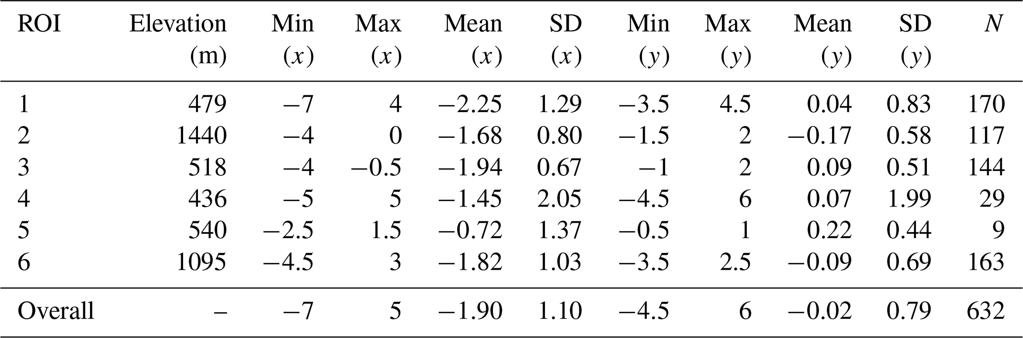
Similar to the results of NOAA-17, the MetOp-A scene mainly presents westward shifts in the across-track direction, indicated by the widely distributed negative values throughout these ROIs (Fig. 6a–f). These shifts are basically concentrated around −2; however, the ROIs 2 and 6 located in the terrain areas show smaller average shifts (−1.68 and −1.82, respectively) than those of ROIs 1 and 3 (−2.25 and −1.94, respectively) over the relatively flat areas. This is understandable since the ROIs 2 and 6 are closer to the nadir area (Fig. 1d). And this aligns with the results from NOAA-17, where the influence of SatZ is also stronger than the terrain effect. Although ROIs 5 and 4 show the smallest average shifts (−0.72 and −1.45, respectively) in the across-track direction, their results may be biased due to the smaller number of analyzed patches. It is interesting to find that ROI 3, which is almost located in the nadir area, still shows the least uncertainty, indicated by the smallest SD of 0.67. Furthermore, all ROIs close to the nadir area are characterized by small SDs (0.8 and 1.03 for ROIs 2 and 6, respectively) compared to ROIs located further away from the nadir area (1.29, 2.05 and 1.37 for ROIs 1, 4 and 5, respectively). These results demonstrate that SatZ plays a crucial role in determining the uncertainty of the shifts in the across-track direction. This conclusion also agrees with previous research conducted by Aguilar et al. (2013). When combining the results of all ROIs (Fig. 6g), the shifts approximately follow a normal distribution, with an average of −1.90 and a standard deviation of 1.1. Most of the patches (94 %) are within the range of ±3 km, and nearly 98 % of them are with shifts less than ±4 km.
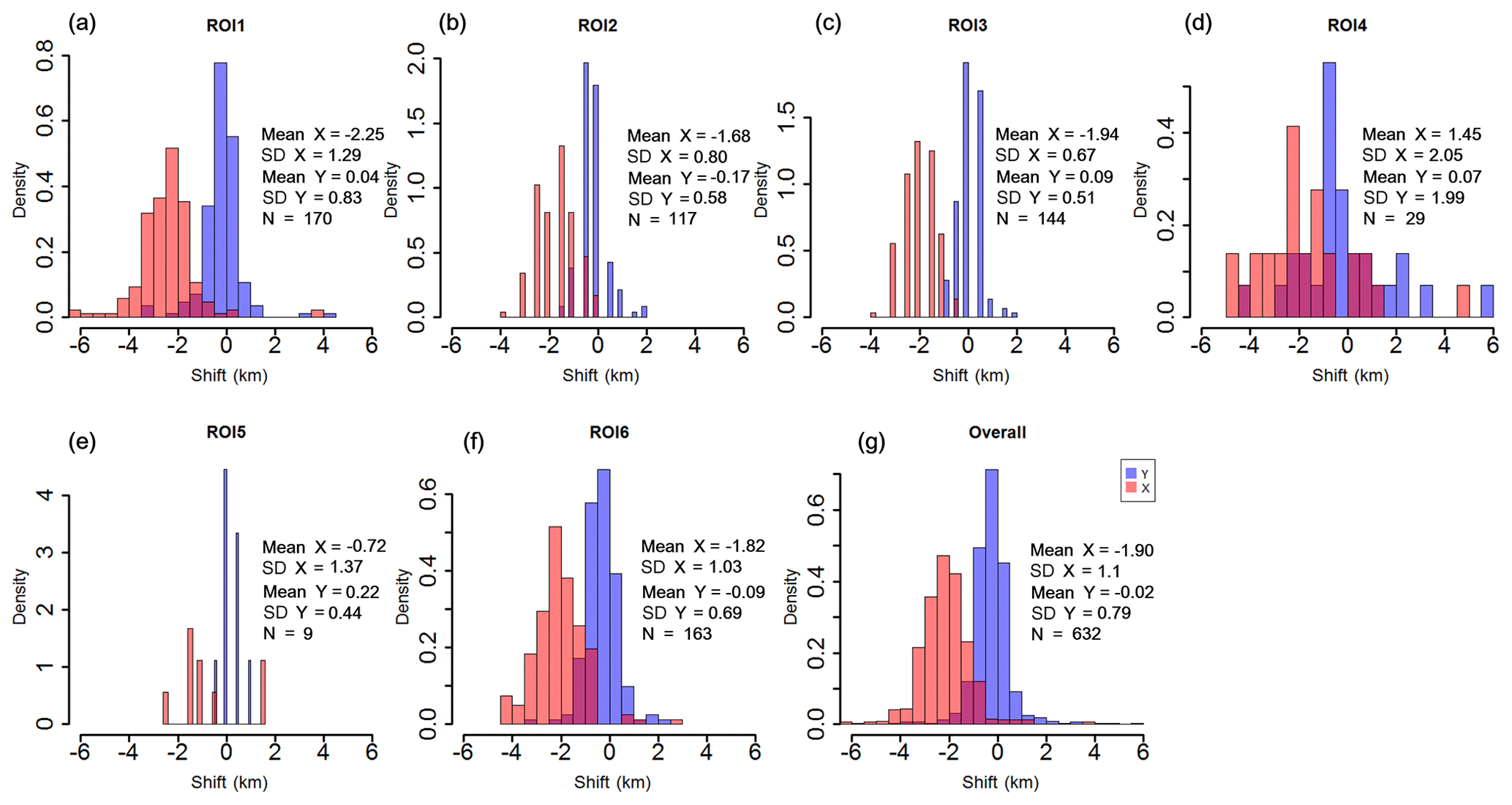
Figure 6The distribution of shifts in the across-track (x, represented by the red histogram) and along-track (y, denoted as the blue histogram) directions over different regions for the MetOp-A scene. The unit of the shift is kilometers. For histograms, density instead of frequency is labeled in the ordinate.
Since ROIs 1–6 on the MetOp-A scene are identical to those on the NOAA-17 scene in terms of spatial extents, their shifts in the across-track direction are generally comparable. When excluding the results of ROIs 4 and 5, the ROIs on the MetOp-A scene generally show larger average shifts but smaller SDs than the NOAA-17 scene in the across-track direction (see Tables 2 and 3). However, it does not necessarily mean that the MetOp-A scene has a smaller uncertainty than the NOAA-17 scene in the across-track direction, because the ROIs on the MetOp-A scene are slightly closer to the nadir area than those on the NOAA-17 scene (Fig. 1b and d). Given the larger SatZ and the smaller average shifts of the NOAA-17 scene, it is reasonable to conclude that the NOAA-17 scene shows a slightly better geolocation accuracy than the MetOp-A scene in the across-track direction.
Looking at the shifts in the along-track direction, the MetOp-A scene does not show strong systematic north or south shifts, but rather a general distribution of the shifts around 0 (Fig. 6a–f). The shifts are generally small within a range of ±1 km, with SDs less than 0.83 except for ROI 4. Furthermore, ROIs 2, 3 and 6 that are located close to the nadir area exhibit smaller SDs than those located further away from the nadir area when excluding ROI 5 due to its very small number of patches. This further indicates that SatZ also determines the uncertainty of shifts in the along-track direction. When combining the results of all ROIs (Fig. 6g), the shifts also display a nearly normal distribution, with an average of −0.02 and a SD of 0.79. Nearly 94 % of the shifts are within the range of ±1 km and almost all of them (98 %) are distributed within the range of ±2 km. It can be found that the shifts in the along-track direction are obviously smaller and more centralized than those in the across-track direction. This can be further confirmed by the consistently smaller SD values in the along-track direction than those in the across-track direction as shown in Table 3.
Table 3Summary of the results for the scene of MetOp-A. The unit of the shift is kilometers.
By comparing Fig. 6a–f with Fig. 5a–f, it becomes obvious that large differences exist between the shifts in the along-track direction of the MetOp-A and NOAA-17 scenes. In the first place, systematic south shifts occur on the NOAA-17 scene but not on the MetOp-A scene. Secondly, the magnitudes of shifts on the MetOp-A scene are generally smaller than those on the NOAA-17 scene, as the former are concentrated around 0 while the latter are concentrated around −1. Thirdly, the distribution of shifts is more centralized for the MetOp-A scene compared to the NOAA-17 scene, except for ROIs 4 and 5. This can be further proven by the smaller SD values for MetOp-A (Table 3) than those for NOAA-17 (Table 2). Therefore, it can be concluded that the MetOp-A scene shows a better geolocation accuracy and less uncertainty than the NOAA-17 scene in the along-track direction.
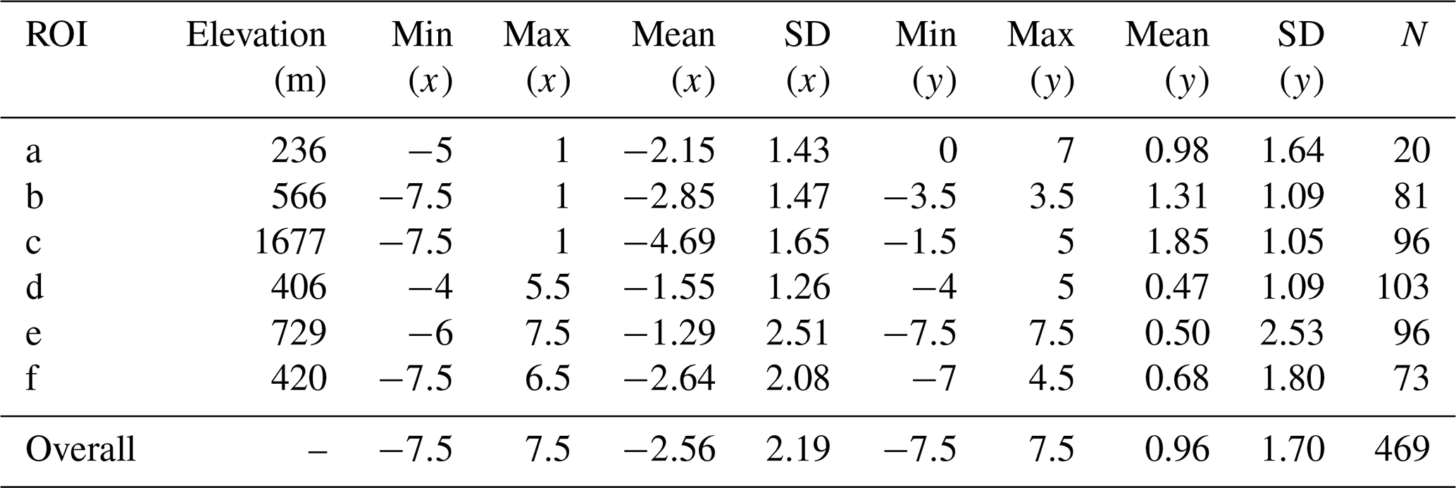
Similar to the scenes of NOAA-17 and MetOp-A, the MetOp-B scene generally shows westward shifts in the across-track direction, indicated by the predominant occurrence of negative values (Fig. 7a–f). Nevertheless, unlike the results for the terrain areas on the NOAA-17 and MetOp-A scenes, the ROI c located in the terrain area on the MetOp-B scene (Fig. 2a) shows the largest shifts throughout these ROIs with an average of −4.69 in the across-track direction. Furthermore, the magnitudes of these shifts are characterized by even larger values than 6 km (Fig. 7c). This is most probably caused by the combined effect of topography and large SatZs (Fig. 2b). Significant terrain effects appear only in the case of SatZs larger than 40∘ as shown in Fig. 2b. This finding agrees with the previous study by Fontana et al. (2009), who demonstrated that the errors in the across-track direction result from the intertwined effects of observation geometry and terrain elevation. Nevertheless, ROI e that is located in the nadir area (Fig. 2d) shows the smallest average shift of −1.29 but the largest standard deviation of 2.51 (Fig. 7e). The largest SD is attributed to the fact that a considerable number of shifts exhibit values of ±6 km. As shown in Fig. 2c, the main reason for these large and unstable shifts may be the presence of thin clouds or cloud shadows in this region. By comparing the results of ROIs d and e with smaller SatZs against ROIs b, c and f with larger SatZs (Fig. 2b and d), it can be stated that the shifts with smaller SatZs are generally weaker than those with larger SatZs (Fig. 7b–f). When combining the results of all ROIs (Fig. 7g), the MetOp-B scene shows an average shift of −2.56 km with a standard deviation of 2.19 in the across-track direction. Only 63 % of the shifts are distributed within the range of ±3 km, and the percentage increases up to 92 % within the range of ±5.5 km.
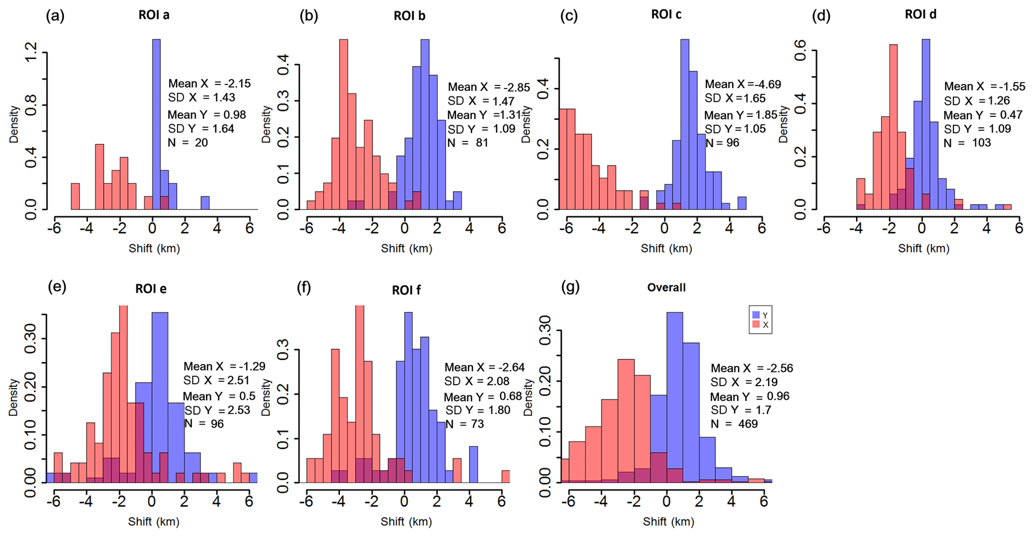
Figure 7The distribution of shifts in the across-track (x, represented by the red histogram) and along-track (y, denoted as the blue histogram) directions over different regions for the MetOp-B scene. The unit of the shift is kilometers. For histograms, density instead of frequency is labeled in the ordinate.
Since the extent of the ROIs in the MetOp-B scene is not consistent with those on NOAA-17 and MetOp-A scenes, only their overall performances in the across-track direction are compared here. By comparing Fig. 7g with Fig. 6g and Fig. 5h, it is obvious that the MetOp-B scene shows larger shifts and greater uncertainties than NOAA-17 and MetOp-A scenes in the across-track direction. This is partly due to the larger range of SatZs of these ROIs and partly due to the worse geolocation accuracy of the MetOp-B scene in the across-track direction.
The MetOp-B scene is dominated by north shifts in the along-track direction, indicated by the predominantly positive shift values (Fig. 7a–f). It is interesting to find that ROI c, which is located at terrain area and with large SatZs, shows the largest shifts with an average of 1.85 km in the along-track direction. Given that terrain does not affect the geolocation accuracy in the along-track direction, the main cause of the largest shift may be the largest SatZ of ROI c among these ROIs. Furthermore, by comparing the results of ROIs d and e with those of ROIs b, c and f, it can be found that the shifts of ROIs with smaller SatZs are more concentrated around 0 (Fig. 7d and e), while the shifts of ROIs with larger SatZs are more widely spread (Fig. 7b, c and f). This shows that the effect of large SatZs on shifts in the along-track direction cannot be neglected. When combining the results of all ROIs, the MetOp-B scene shows shifts with an average of 0.96 and a standard deviation of 1.7. Only 52 % of the shifts are distributed within the range of ±1 km, and the percentage increases up to 92 % for the range of ±3 km.
It can be seen that the shifts in the along-track direction are still significantly smaller than those in the across-track direction. Furthermore, the uncertainties of the shifts in the along-track direction are generally smaller than those in the across-track direction, when excluding the results of ROI a due to its limited number of patches (Table 4). This further verifies that after removing clock drift errors, the geolocation errors in the along-track direction are generally more accurate and have fewer uncertainties than the across-track direction.
Table 4Summary of the results for the scene of MetOp-B. The unit of the shift is kilometers.
The comparison of Fig. 7g with Figs. 6g and 5h reveals that the MetOp-B scene is significantly inferior to the MetOp-A scene in terms of the geolocation accuracy in the along-track direction, with the former being concentrated around 1 and the latter around 0. Furthermore, the uncertainty of the shifts of the MetOp-B scene (SD =1.7) is much larger than that of the MetOp-A scene (SD =0.79). As for the performance of the MetOp-B scene relative to the NOAA-17 scene, it can be found that they are comparable with regard to the magnitude as well as the distribution of the shifts in the along-track direction. However, the MetOp-B scene shows larger uncertainties than NOAA-17.
From the results above, it can be concluded that NOAA-17 and MetOp-A scenes show distinct advantages over the MetOp-B scene in both directions. However, the NOAA-17 scene is slightly better than the MetOp-A scene in the across-track direction, with average shifts of −1.69 for NOAA-17 and −1.90 for MetOp-A, which are both greatly lower than for MetOp-B (−2.56). But the MetOp-A scene shows a distinct advantage over NOAA-17 in the along-track direction, with an average shift of −0.02 for MetOp-A and −0.7 for NOAA-17, which are both lower than for MetOp-B (0.96). In addition to the magnitudes of their shifts, the MetOp-B scene also shows larger uncertainties than NOAA-17 and MetOp-A scenes in both directions.
4.2 The potential influence factors
From the above results, it is known that SatZ plays an important role in determining the geolocation accuracy of the satellite scene. To investigate how and to what extent it influences the geolocation accuracy, Fig. 8 displays the shifts in both directions as a function of SatZ for all three satellites. Furthermore, the influences of latitude and longitude on geolocation accuracy are also explored.
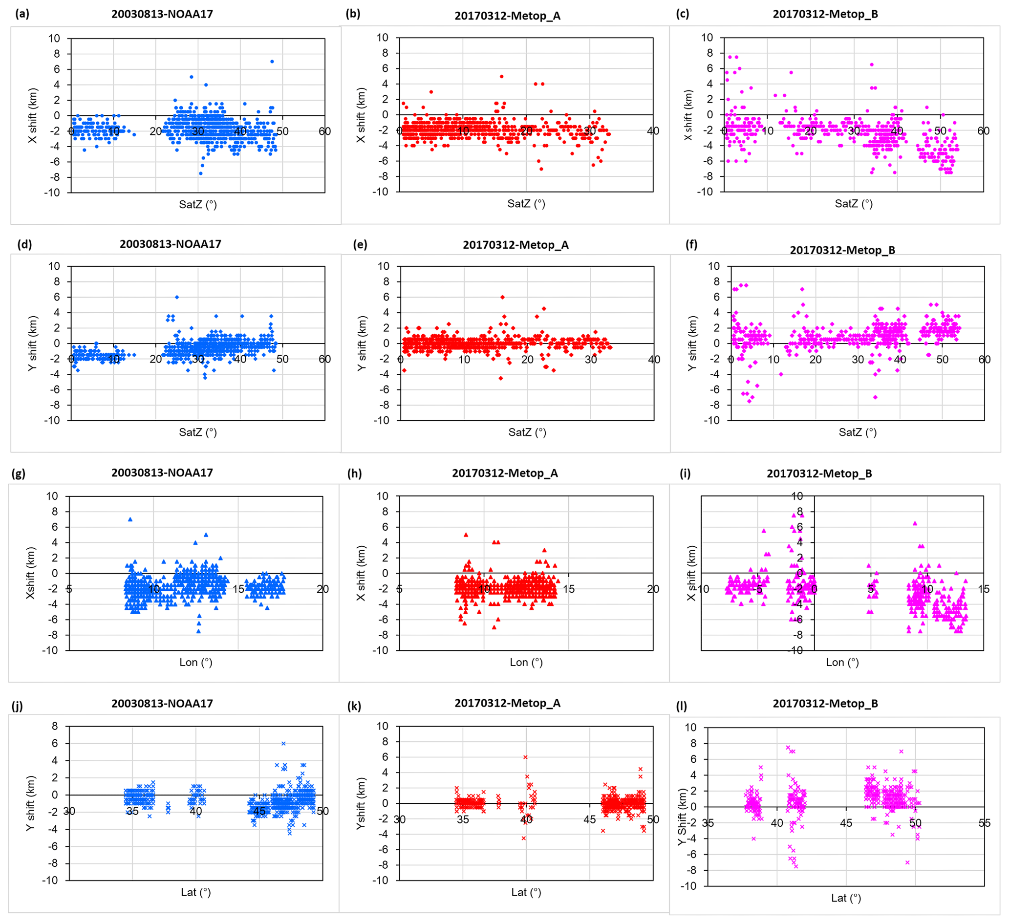
Figure 8Influence of SatZ on the geolocation accuracy in the across-track (a–c) and along-track (d–f) directions. Panels (g–i) and (j–l) describe the influence of longitude and latitude on the geolocation accuracy in the across-track and along-track directions, respectively. The left column indicates results of NOAA-17 (blue), middle MetOp-A (red) and right MetOp-B (pink) scenes.
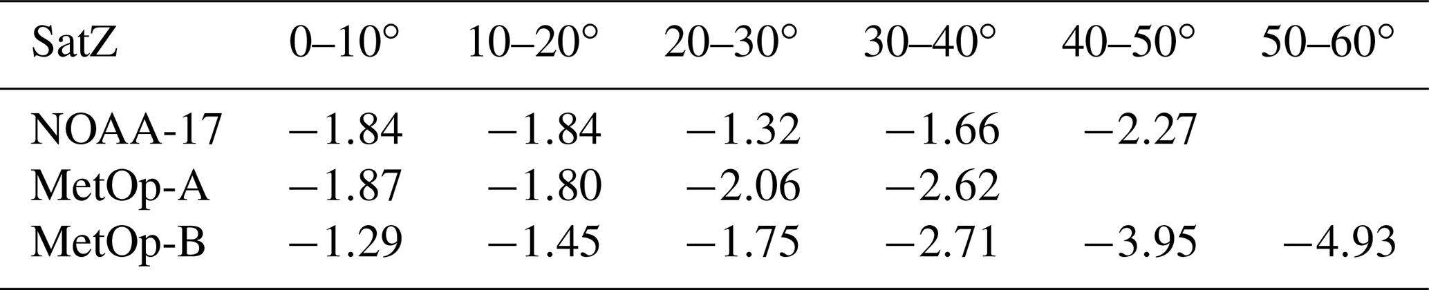
As shown in Fig. 8a–c, it can be seen that the shifts in the across-track direction vary considerably for all SatZs, and this is particularly evident in the results of MetOp-B (Fig. 8c). This demonstrates that besides the SatZ effects, the geolocation accuracy is also influenced by other factors. Furthermore, the spread at each fixed SatZ tends to become larger at larger SatZs (larger than 20∘) (Fig. 8a–b). The large variability of MetOp-B scene shifts at small SatZs (less than 20∘) (Fig. 8c) is mainly due to the effect of thin cloud or cloud shadow as explained before. Despite the dispersion of the shifts for all SatZs, it can still be found that the shifts in the across-track direction do not change much when the SatZ is less than 20∘ (Fig. 8a–b and Table 5). A slightly decreasing trend (increasing trend of the magnitude) can be observed from 20 to 40∘ (Table 5) and becomes more apparent at SatZs larger than 40∘ (Fig. 8c and Table 5). Furthermore, it can be found that for small SatZs (less than 20∘) the shifts in the across-track direction are generally concentrated around 2 km for NOAA-17 and MetOp-A scenes (Fig. 8a–b). With increasing SatZ, the largest magnitudes of shifts become larger but basically stay within the range of 4 km for SatZs smaller than 40∘. For even larger SatZs (larger than 40∘), the magnitude of shifts can reach 6 km for the NOAA-17 scene and 8 km for the MetOp-B scene. From these results, it can be inferred that the SatZ has a considerable effect on both the magnitude and uncertainty of the shifts in the across-track direction. The larger SatZ generally contributes to larger shifts and uncertainties in the across-track direction. Furthermore, it can be inferred that the GAC data with SatZs less than 40∘ should be preferred in applications.
Compared to the shifts in the across-track direction (Fig. 8a–c), the shifts in the along-track direction show smaller variability at each fixed SatZ (Fig. 8d–f). From Fig. 8d–e, it can be seen that the shifts in the along-track direction are relatively stable at each level of SatZ for SatZs smaller than 15∘, but they become more variable for greater SatZs. A similar phenomenon can be observed in Fig. 8f, where the shifts are relatively stable with SatZs ranging from 20 to 35∘ but become more variable at each level of SatZ with its values larger than 35∘. It is noteworthy that the wide spread of shifts with SatZs less than 20∘ is mainly caused by cloud contamination. These results confirm the influence of larger SatZs on the uncertainty of shifts in the along-track directions. It is interesting to find that the magnitudes of NOAA-17 scene shifts with small SatZs (less than 20∘) are even larger than those with larger SatZs (larger than 20∘) (Fig. 8d). Conversely, the magnitudes of MetOp-B scene shifts with smaller SatZs (20–35∘) are smaller than those with larger SatZs (larger than 35∘) (Fig. 8f). Nevertheless, all three sensors have in common that they do not show clear change with SatZs smaller than 20∘ for NOAA-17 and smaller than 35∘ for MetOp-A and MetOp-B (Fig. 8d–f). For SatZs larger than these values, shifts exhibit a slightly decreasing trend for NOAA-17 (Fig. 8d) and an increasing trend for MetOp-B (Fig. 8f). From these results, it can be stated that the influences of large SatZs on the magnitude of shifts in the along-track direction are probably intertwined with other factors.
Table 5The mean shift for each range of SatZ in the across-track direction. The unit of the shift is kilometers.
For NOAA-17, the shifts tend to be smaller with the longitudinal range of 10–15∘ and become larger outside this range (Fig. 8g). The MetOp-A scene does not show apparent change with longitude between 8 and 15∘ and neither does MetOp-B within the range between −8 and 0∘ (Fig. 8h and i, respectively). However, MetOp-B presents a clear decreasing trend (an increasing trend in magnitude) for longitudes larger than 5∘. Given the fact that the longitude of the nadir area is distributed between 10 and 15∘ for NOAA-17, 8 and 15∘ for MetOp-A and −8 and 0∘ for MetOp-B (Figs. 1b and d, 2b and d), it can be concluded that the influence of longitude on the shifts in the across-track direction is related to the longitude of nadir area of the satellite, as it shows almost no influence in the nadir area. The influence increases with the difference of the longitude relative to that of the nadir area. This is understandable, as the influence of longitude is equivalent to that of SatZ in the across-track direction.
The variation in the shifts (in the along-track direction) with latitude also depends on the situation (Fig. 8j–l). The magnitudes of shifts with larger latitude (larger than 45∘) are generally greater than those with smaller latitude (less than 40∘) on the NOAA-17 (Fig. 8j) and MetOp-B scenes (Fig. 8l). This is not visible for the MetOp-A scene (Fig. 8k), where the shifts exhibit almost no change with latitude. This can be attributed to the fact that the clock drift errors are corrected more thoroughly for the MetOp-A satellite than NOAA-17 and MetOp-B satellites. Furthermore, the MetOp satellites have an onboard stabilization to keep them in the right position and orientation in orbit compared to the NOAA satellites.
The AVHRR GAC test data in this paper draw on datasets from the ESA CCI cloud project (http://www.esa-cloud-cci.org/, last access: 30 October 2018) where the data availability is also indicated (https://doi.org/10.5676/DWD/ESA_Cloud_cci/AVHRR-AM/V002, Stengel et al., 2017). And the MOD13A1 V006 data can be downloaded via https://ladsweb.modaps.eosdis.nasa.gov/ (last access: 17 November 2018) (https://doi.org/10.5067/MODIS/MOD13A1.006, Didan, 2015).
The geometric accuracy of satellite data is crucial for most applications as geometric inaccuracy can bias the obtained results. Therefore, the assessment of the geolocation accuracy is important to provide satellite data of high quality enabling successful applications. In this study, a correlation-based patch matching method was proposed to characterize and quantify the AVHRR GAC geo-location accuracy. This method presented here yields significant advantages over existing approaches and enables the achievement of a sub-pixel geo-positioning accuracy of coarse-resolution scenes. It is free from the impact of false detection due to the influence of mixed pixels and not limited to a certain landmark (e.g., shoreline) and therefore enables a more comprehensive geometric assessment. This method was utilized to characterize the geolocation accuracy of AVHRR GAC scenes from the NOAA-17, MetOp-A and MetOp-B satellites.
The study is based on several ROIs comprising numerous patches over different land cover types, latitudes and topographies. The scenes from these satellites all present westward shifts in the across-track direction, with an average shift of −1.69 km and a SD of 1.32 km for NOAA-17, −1.9 km and 1.1 km, respectively, for MetOp-A, and −2.56 and 2.19 km, respectively, for MetOp-B. In regard to the shifts in the along-track direction, NOAA-17 generally shows southward shifts with an average of −0.7 km and a SD of 1.01 km. By contrast, MetOp-B mainly presents northward shifts with an average of 0.96 km and a SD of 1.70 km. The MetOp-A scene shows a distinct advantage over NOAA-17 and MetOp-B in the along-track direction without obvious shifts, indicated by the average of −0.02 km and a SD of 0.79 km. Generally, the MetOp-B scene is inferior to the NOAA-17 and MetOp-A scenes, with larger shifts and uncertainties in both directions. Despite the variation in shifts due to various factors (e.g., SatZ, topography), more than 90 % of the AVHRR GAC data across-track errors are within ±3 km for NOAA-17 and MetOp-A and ±5.5 km for MetOp-B. Along-track errors are within ±2 km for NOAA-17, ±1 km for MetOp-A and ±3 km for MetOp-B for more than 90 % of the test data. It is important to note that since these satellites show different shifts, using the combined data from NOAA-17 and MetOp will result in additional uncertainty in time series applications.
From the results above, it can be found that the geolocation accuracy in the along-track direction is always higher and with fewer uncertainties than the across-track direction, which is consistent with previous related studies. This is understandable since the GAC dataset from the ESA cloud CCI project has been corrected for clock drift errors but has no ortho-correction, which is not feasible due to the onboard sampling characteristics. SatZ plays a decisive role in determining the magnitude as well as the uncertainty of the shifts in the across-track direction. Larger SatZ generally induce greater shifts and uncertainties in this direction. The combined effect of SatZ and topography on geolocation accuracy in the across-track direction has also been shown. And significant terrain effects appear only in the case of large SatZs (>40∘ for this study). It is important to note that the effect of SatZ on the magnitude and uncertainty of shifts in the along-track direction is not negligible. But this effect is likely to be intertwined with other factors. The impact of longitude on the shifts in the across-track direction is equivalent to that of SatZ, while the effect of latitude is related to the degree of how the clock drift errors are corrected. It was found that the clock drift errors are more thoroughly corrected for MetOp-A than NOAA-17 and MetOp-B.
Although this assessment was only conducted for a single scene of each satellite, the highly variable ROIs take the influential factors of geometric accuracy into account. Therefore, the presented conclusions are transferable to other regions or seasons. However, it is noteworthy that this method is not applicable to homogeneous surfaces (e.g., water, desert), where the correlations are almost the same in any simulated displacement cases. In general, this study provides an important preliminary geolocation assessment for AVHRR GAC data. It is a first step towards a more precise geolocation and thus improves application of coarse-resolution satellite data. For instance, it identifies the threshold of SatZ under which the GAC data should be preferred in applications. Furthermore, the CPMM geolocation assessment method proposed by this study is also applicable to other coarse-resolution satellite data.
XW was responsible for the main research ideas and writing the manuscript. KN contributed to the data collection. SW contributed to the manuscript organization. All the authors thoroughly reviewed and edited this paper.
The authors declare that they have no conflict of interest.
The authors are grateful to the ESA CCI (Climate Change Initiative) cloud project team (Martin Stengel, Rainer Hollmann) for making the datasets available for this study.
This work was jointly supported by the National Key R&D Program of China (grant nos. SQ2018YFB0504804 and 2018YFA0605503) and the National Natural Science Foundation of China (grant no. 41801226).
This paper was edited by Prasad Gogineni and reviewed by two anonymous referees.
Aguilar, M. A., del Mar Saldana, M., and Aguilar, F. J.: Assessing geometric accuracy of the orthorectification process from GeoEye-1 and WorldView-2 panchromatic images, Int. J. Appl. Earth Obs., 21, 427–435, 2013.
Aksakal, S. K.: Geometric accuracy investigations of SEVIRI high resolution visible (HRV) level 1.5 Imagery, Remote Sens., 5, 2475–2491, 2013.
Aksakal, S. K., Neuhaus, C., Baltsavias, E., and Schindler, K.: Geometric quality analysis of AVHRR orthoimages, Remote Sens., 7, 3293–3319, 2015.
Alcaraz-Segura, D., Chuvieco, E., Epstein, H. E., Kasischke, E. S., and Trishchenko, A.: Debating the greening vs. browning of the North American boreal forest: differences between satellite datasets, Glob. Change Biol., 16, 760–770, 2010.
Arnold, G. T., Hubanks, P. A., Platnick, S., King, M. D., and Bennartz, R.: Impact of Aqua misregistration on MYD06 cloud retrieval properties, Proceeding of MODIS Science Team Meeting, Washington, DC, USA, 26–28 January 2010.
Bennartz, R.: On the use of SSM/I measurements in coastal regions, J. Atmos. Ocean. Tech., 16, 417–431, 1999.
Bicheron, P., Amberg, V., Bourg, L., Petit, D., Huc, M., Miras, B., and Leroy, M.: Geolocation Assessment of MERIS GlobCover Orthorectified Products, IEEE T. Geosci. Remote, 49, 2972–2982, 2011.
Cihlar, J., Latifovic, R., Chen, J., Trishchenko, A., Du, Y., Fedosejevs, G., and Guindon, B.: Systematic corrections of AVHRR image composites for temporal studies, Remote Sens. Environ., 89, 217–233, 2004.
Delbart, N., Le Toan, T., Kergoat, L., and Fedotova, V.: Remote sensing of spring phenology in boreal regions: A free of snow-effect method using NOAA–AVHRR and SPOT–VGT data (1982–2004), Remote Sens. Environ., 101, 52–62, 2006.
Devasthale, A., Raspaud, M., Schlundt, C., Hanschmann, T., Finkensieper, S., Dybbroe, A., and Karlsson, K. G.: PyGAC: an open-source, community-driven Python interface to preprocess more than 30-year AVHRR Global Area Coverage (GAC) data, 2016.
Didan, K.: MOD13A1 MODIS/Terra Vegetation Indices 16-Day L3 Global 500m SIN Grid V006 [Data set], NASA EOSDIS LP DAAC, available at: https://ladsweb.modaps.eosdis.nasa.gov/ (last access: 15 January 2019), https://doi.org/10.5067/MODIS/MOD13A1.006, 2015.
Fontana, F. M., Trishchenko, A. P., Khlopenkov, K. V., Luo, Y., and Wunderle, S.: Impact of orthorectification and spatial sampling on maximum NDVI composite data in mountain regions, Remote Sens. Environ., 113, 2701–2712, 2009.
Han, Y., Weng, F., Zou, X., Yang, H., and Scott, D.: Characterization of geolocation accuracy of Suomi NPP advanced technology microwave sounder measurements, J. Geophys. Res.-Atmos., 121, 4933–4950, 2016.
Hoffman, L. H., Weaver, W. L., and Kibler, J. F.: Calculation and accuracy of ERBE scanner measurement locations, NASA Tech. Pap. Rep. NASA/TP-2670, NASA Langley Research Center, Hampton, Virginia, 34 pp., 1987.
Hollmann, R., Merchant, C., Saunders, R., Downy, C., Buchwitz, M., Cazenave, A., Chuvieco, E., Defourny, P., Leeuw, G. de, Forsberg, R., Holzer-Popp, T., Paul, F., Sandven, S., Sathyendranath, S., van Roozendael, M., and Wagner W.: The ESA Climate Change Initiative: satellite data records for essential climate variables, B. Am. Meteorol. Soc., 94, 1541–1552, https://doi.org/10.1175/BAMS-D-11-00254.1, 2013.
Hori, M., Sugiura, K., Kobayashi, K., Aoki, T., Tanikawa, T., Kuchiki, K., and Enomoto, H.: A 38-year (1978–2015) Northern Hemisphere daily snow cover extent product derived using consistent objective criteria from satellite-borne optical sensors, Remote Sens. Environ., 191, 402–418, 2017.
Khlopenkov, K. V., Trishchenko, A. P., and Luo, Y.: Achieving subpixel georeferencing accuracy in the Canadian AVHRR processing system, IEEE T. Geosci. Remote, 48, 2150–2161, 2010.
Kidwell, K. B.: NOAA Polar Orbiter Data (POD) User's Guide, November 1998 revision, available at: http://www2.ncdc.noaa.gov/docs/podug/ (last access: 15 January 2019), 1998.
Lee, T. Y. and Kaufman, Y. J.: Non-Lambertian effects on remote sensing of surface reflectance and vegetation index, IEEE T. Geosci. Remote, 24, 699–708, 1986.
Moulin, S., Kergoat, L., Viovy, N., and Dedieu, G.: Global-scale assessment of vegetation phenology using NOAA/AVHRR satellite measurements, J. Climate, 10, 1154–1170, 1997.
Pouliot, D., Latifovic, R., and Olthof, I.: Trends in vegetation NDVI from 1 km AVHRR data over Canada for the period 1985–2006, Int. J. Remote Sens., 30, 149–168, 2009.
Stengel, M., Sus, O., Stapelberg, S., Schlundt, C., Poulsen, C., and Hollmann, R.: ESA Cloud Climate Change Initiative (ESA Cloud_cci) data: Cloud_cci AVHRR-AM L3C/L3U CLD_PRODUCTS v2.0, Deutscher Wetterdienst (DWD), https://doi.org/10.5676/DWD/ESA_Cloud_cci/AVHRR-AM/V002, 2017.
Stöckli, R. and Vidale, P. L.: European plant phenology and climate as seen in a 20 year AVHRR land-surface parameter dataset, Int. J. Remote Sens., 25, 3303–3330, 2004.
Takagi, M.: Precise geometric correction for NOAA and GMS images considering elevation effects using GCP template matching and affine transform, Proceedings of SPIE Conference on Remote Sensing, Image and Signal Processing for Remote Sensing IX, Vol. 5238, 132–141, Barcelona, Spain, 2004.
Van, A., Nakazawa, M., and Aoki, Y.: Highly accurate geometric correction for NOAA AVHRR data, available at: http://cdn.intechopen.com/pdfs/10391/InTech Highly_accurate_geometric_correction_for_ noaa_ avhrr_ data.pdf (last access: 15 January 2019), 2008.
Wang, L., Tremblay, D. A., Han, Y., Esplin, M., Hagan, D. E., Predina, J., Suwinski, L., Jin, X., and Chen, Y.: Geolocation assessment for CrIS sensor data records. J. Geophys. Res.-Atmos., 118, 12–690, 2013.
WMO and UNEP: Systematic observation requirements for satellite-based products for climate-Supplemental details to the satellite-based component of the “Implementation Plan for the Global Observing System for Climate in Support of the UNFCCC”, Technical Report GCOS-107, WMO/TD No 1338, 2006.
Wolfe, R. E., Nishihama, M., Fleig, A. J., Kuyper, J. A., Roy, D. P., Storey, J. C., and Patt, F. S.: Achieving sub-pixel geolocation accuracy in support of MODIS land science, Remote Sens. Environ., 83, 31–49, 2002.
Wolfe, R. E., Lin, G., Nishihama, M., Tewari, K. P., Tilton, J. C., and Isaacman, A. R.: Suomi NPP VIIRS prelaunch and on-orbit geometric calibration and characterization, J. Geophys. Res.-Atmos., 118, 11508–11521, 2013.