the Creative Commons Attribution 4.0 License.
the Creative Commons Attribution 4.0 License.
 | 18 Feb 2020
Glaciers and climate of the Upper Susitna basin, Alaska
Regine Hock
Gabriel Wolken
Erin Whorton
Caroline Aubry-Wake
Juliana Braun
Alessio Gusmeroli
Will Harrison
Andrew Hoffman
Anna Liljedahl
Jing Zhang
Extensive field observations were conducted in the Upper Susitna basin, a 13 289 km2 glacierized catchment in central Alaska in 2012–2014. This paper describes the comprehensive data set of meteorological, glacier mass balance, snow cover, and soil measurements, as well as the data collection and processing. Results are compared to similar observations from the 1980s. Environmental lapse rates measured with weather stations between about 1000 and 2000 m a.s.l. were significantly lower over the glaciers than the non-glacierized areas. Glacier-wide mass balances shifted from close to balanced in 1981–1983 to less than −1.5 m w.e. yr−1 in 2012–2014. Winter snow accumulation measured with ablation stakes on the glaciers closely matched observations from helicopter-borne radar. Soil temperature measurements across the basin showed that there was no permafrost in the upper 1 m of the soil column. The data produced by this study are available at: https://doi.org/10.14509/30138 (Bliss et al., 2019) and will be useful for hydrological and glaciological studies including modeling efforts.
- Article
(18590 KB) - Full-text XML
- BibTeX
- EndNote


Climate change is projected to have significant impacts on future water resources. In snow- and glacier-dominated catchments the response is strongly affected by changes in snow and glacier storage (Bliss et al., 2014; Huss and Hock, 2018). Changes in precipitation amounts and seasonality, air temperature, glacier mass balance, and vegetation type all contribute to changes in river runoff and water availability. Understanding present-day relationships among these contributing factors can help improve projections of future river runoff. However, long-term spatially representative hydrometeorological observations in mountain regions are scarce, making it difficult to study these relationships or calibrate and validate modeling studies.
The headwaters of the Susitna River's watershed in central Alaska provide an interesting case study of these factors. During the 1980s intensive glaciologic and hydrologic fieldwork was conducted in the Upper Susitna basin in connection with a proposed hydroelectric dam on the Susitna River (Clarke, 1991; R&M Consultants and Harrison, 1981; Clarke et al., 1985). The dam was not built, but when the proposal resurfaced approximately 30 years later (Susitna-Watana Hydroelectric Project, http://www.susitna-watanahydro.org/, last access: 6 December 2018), we performed extensive field measurements in the same area. Our work combined field measurements with glacier runoff modeling to project how future glacier mass changes influence water flow to the proposed dam. This paper focuses on the measurements, while the modeling results have been described in Wolken et al. (2015).
More than 100 glaciers flow down the southern flanks of the central Alaska Range into the three forks of the Upper Susitna River (Fig. 1). The glaciers provide a significant portion of the total runoff within the Upper Susitna drainage. It is well documented that glaciers across Alaska are currently retreating (Gardner et al., 2013; Luthcke et al., 2013). Changes to the timing and amount of runoff due to continued melting of glaciers have been projected to occur worldwide (Bliss et al., 2014; Huss and Hock, 2018). Therefore, it is important to understand how changes to the Upper Susitna basin glaciers and river flow could affect dam operations and environmental resources.
This paper describes the data collected during the 2012–2014 field campaign detailing the instrumentation, method of deployment, and results for each set of data. Observations included meteorological variables, glacier mass balance, snow depth and density, and soil type and temperature. Where possible we also compare the data with the results from the 1980s field campaign.
The watershed above the proposed Susitna-Watana dam (62.822523∘ N, 148.538986∘ W; henceforth referred to as the Upper Susitna basin) covers an area of 13 289 km2 with elevation spanning from 450 to 4200 m above sea level (a.s.l., Fig. 1). About 4 % of the basin is glacierized. The total glacier area is 678.4 km2 according to the Randolph Glacier Inventory version 6.0 (Pfeffer et al., 2014; Kienholz et al., 2015), which is based on satellite imagery from 3 July 2009. Modern glaciers are well within the limit of the Late Wisconsinan glacial advance (20–25 ka), when this part of the Alaska Range hosted the northern extent of the Cordilleran Ice Sheet (Kauman and Manley, 2004).
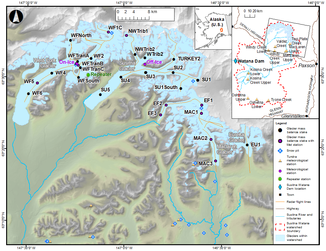
Figure 1Map of study area including measurement locations. From west to east, the major glaciers are West Fork Glacier (stations with the prefix WF), Susitna Glacier (SU), East Fork Glacier (EF), Maclaren Glacier (MAC), and Eureka Glacier (EU). The main map focuses on the glacierized portion of the basin, the large inset shows the whole Upper Susitna basin which drains to the proposed dam site, and the small inset shows the basin in the context of the state of Alaska.
Almost all of the basin's glacier area is found in the Alaska Range whose highest ridges and peaks form the basin's northern boundary. This area is characterized by high relief (Fig. 1). Most glaciers (in total 127) in the study area are located in the Alaska Range, but a few small glaciers exist in the Talkeetna Mountains which form the southwest boundary of the basin.
The glacier monitoring work focused on the five largest glaciers in the Alaska Range: West Fork Glacier (193.4 km2), Susitna Glacier (209.6 km2), East Fork Glacier (39.8 km2), Maclaren Glacier (56.5 km2), and Eureka Glacier (34.0 km2). Apart from a former tributary of the West Fork Glacier (33.0 km2), which is now disconnected, the remaining glaciers are smaller than 7 km2. Ninety-three of the 127 glaciers in the Alaska Range are smaller than 1 km2 and their total area is 32.3 km2. Using a volume–area scaling relationship (Bahr et al., 1997), we estimate a total glacier volume of 137 km3 for the Upper Susitna basin. We use scaling coefficients for mountain glaciers (c=0.2055 m3−2γ, γ=1.375, Radić et al., 2008). If we assume an ice density of 900 kg m−3, this represents 123 Gt of ice. Some of the larger glacier termini reach elevations between 800 and 900 m a.s.l.
The nine glaciers in the Talkeetna Mountains draining to the Susitna river have a combined area of 8.9 km2. The largest glacier, located at the head of the Black River, is 7.3 km2. The total glacier volume is less than 0.6 km3 (0.5 Gt).
Significant portions of the large glaciers in the Alaska Range are covered by rock debris. Debris of sufficient thickness, like that found on West Fork and Susitna glaciers in particular, has an insulating effect on the ice underneath, reducing the amount of ice melt compared to bare ice areas (Scherler et al., 2011). A Landsat image from 15 September 2010 revealed that the disconnected tributary of West Fork Glacier was 7 % covered by debris. Debris covered 18 % of West Fork Glacier, 26 % of Susitna Glacier, 3 % of East Fork Glacier, 6 % of Maclaren Glacier, and 7 % of Eureka Glacier.
Wastlhuber et al. (2017) determined glacier area and mass changes of the basin’s glaciers between 1951 and 2010 and found substantial glacier retreat and mass losses. During this period the glaciers lost an area of 128±15 km2 (16 %) and thinned on average by 0.41±0.07 m yr−1. The average thinning rate almost tripled (1.20±0.25 m yr−1) during the later period 2005–2010. Using satellite imagery, the average equilibrium (1999–2015) line altitude was found to be at 1745±88 m a.s.l.
Both Susitna and West Fork glaciers have a history of surging. Surge-type glaciers experience episodic acceleration of flow at many times their normal velocities, transferring large amounts of ice to lower elevation, and they usually result in rapid terminus advance and outburst floods. The last known Susitna Glacier surge occurred in 1951 or 1952, with a pronounced terminus advance and a maximum ice movement of about 4 km (Post, 1960; Clarke, 1991). West Fork Glacier surged in 1935 or 1937 and again from 1987 to 1988. The latter produced a maximum ice displacement of 4 km and a surface elevation increase of up to 120 m observed near the terminus (Clarke, 1991; Harrison et al., 1994). Harrison et al. (1994) report that during the termination of the 1987–1988 surge that runoff and sediment fluxes sharply increased from the glacier to the Susitna River.
During quiescent periods, mean annual glacier surface velocities in the Upper Susitna basin are estimated to range from 0 to 0.73 m d−1 (Burgess et al., 2013); the highest velocities occur on Susitna and West Fork glaciers. Some glaciers experience brief periods of acceleration in spring, which have been linked to enhanced basal lubrication caused by meltwater (MacGregor et al., 2005; Bartholomaus et al., 2008). Periods of deceleration in late summer have been connected to warm summers and greater meltwater production (Sundal et al., 2011).
The non-glacierized part of the basin is characterized by sparse vegetation and little human development. The southeastern part of the watershed is characterized by low relief, numerous lakes, and open spruce forest. The largest lakes are Susitna Lake and Lake Louise. A low divide to the south and east separates the Susitna basin from the Copper River and its tributaries.
The majority of the area draining into the proposed dam is estimated to be underlain by discontinuous and continuous permafrost (Fig. 2). Maximum depth to the base of permafrost near the Maclaren River junction with the Susitna River is about 200 m (United States Army Corps of Engineers, 1975), while it is 40 m at Gulkana, approximately 50 km southeast of the basin (Romanovsky et al., 2010). Permafrost affects water runoff, soil temperature, vegetation, and soil carbon fluxes. These factors have complex interactions with climate change.
Nearby weather stations with long-term records include Talkeetna Airport (west of the basin, 1067 m a.s.l.) and Gulkana Airport (east of the basin, 467 m a.s.l.). Annual mean temperature for the period 1985–2014 at Talkeetna was 1.4 ∘C and at Gulkana −1.5 ∘C (http://ncdc.noaa.gov, last access: 6 December 2018). Precipitation averaged 710 mm yr−1 at Talkeetna and 288 mm yr−1 at Gulkana.
Flow of the Susitna River at Gold Creek (62∘46′04′′ N, 149∘41′28′′ W, downstream of the basin considered in this paper) was 8.8±1.2 km3 yr−1 (mean ± standard deviation), or 277.8±36.8 m3 s−1, over the period 1950–2015 with a measurement hiatus from 1997 to 2000. Peak flow was usually in mid-June.
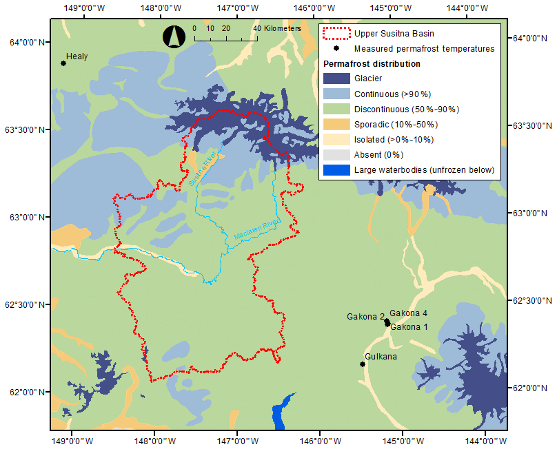
Figure 2Distribution of permafrost in study area (modified after Jorgenson et al., 2008).
Climate exerts the primary influence on river runoff and glacier mass balance. The meteorological and climatological knowledge of mountainous areas of south-central Alaska, including the Upper Susitna basin, is generally poor, largely due to the sparse and poorly distributed data (no in situ data available from high elevations) and the lack of consistent, long-term measurements. To improve the coverage, we strategically placed two energy balance weather stations in the Alaska Range and 25 simple weather stations throughout the entire watershed (Figs. 1 and 3). Table A1 lists the location and elevation of all meteorological stations used in this study.
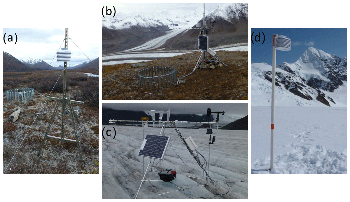
Figure 3Photos of employed weather stations: (a) example of a tundra station, (b) Off-Ice station perched on a Susitna Glacier nunatak, (c) On-Ice station located on West Fork Glacier, (d) example of simple glacier station.
3.1 Energy balance weather stations
3.1.1 Instrumentation
Two energy balance weather stations were installed in the upper part of the basin, one on the West Fork Glacier and one on a ridge between the two branches of the Susitna Glacier (Fig. 3).
Table 1Sensors used for the energy balance weather stations (On-Ice and Off-Ice).
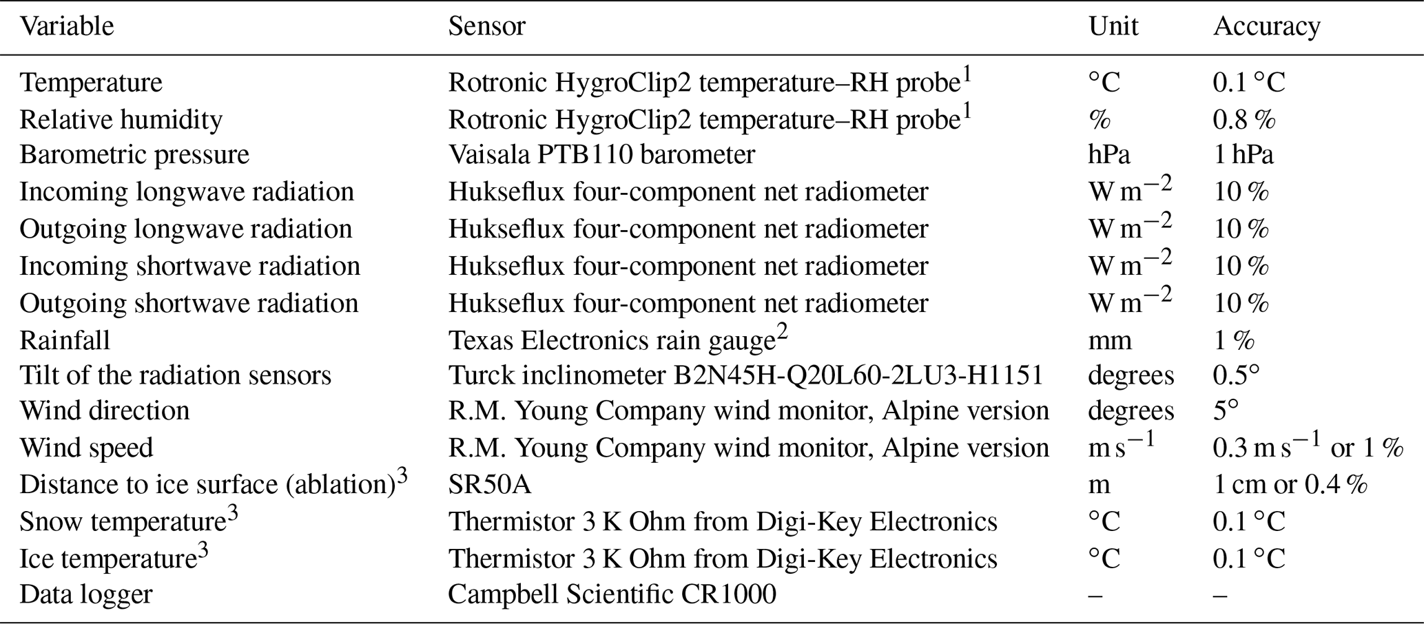
1 Shielded with a R.M. Young Company 10-plate Gill shield. 2 Installed at the Off-Ice station at 0.6 m (top of gauge to ground surface) and shielded with a NovaLynx Alter-type rain gauge wind screen. Installed at the On-Ice station on top of the instrument arm at 2 m above the surface and unshielded (Fig. 3). Gauges were not heated and hence gave most accurate results when precipitation was liquid rather than solid. 3 Only at the On-Ice station.
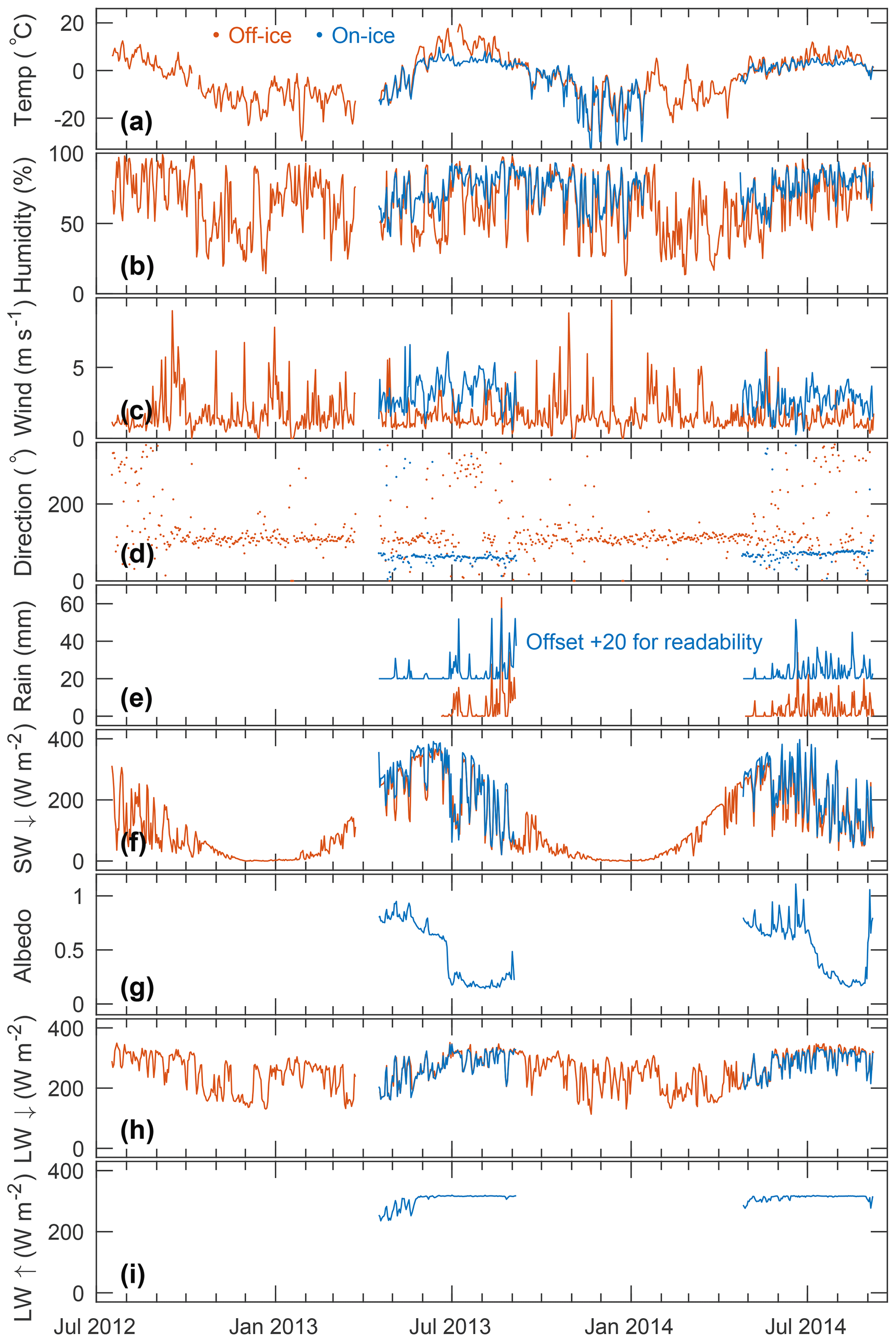
Figure 4Meteorological data from the On-Ice and Off-Ice stations from July 2012 to September 2014. (a) Daily temperature, (b) relative humidity, (c) wind speed, (d) wind direction, (e) precipitation, (f) incoming shortwave (SW) radiation, (g) albedo, (h) incoming longwave (LW) radiation, and (i) outgoing LW radiation. All values are daily means except for precipitation, which is the daily sum. Data gaps occur in winter when some sensors were removed. The On-Ice temperature–humidity sensor was buried in the snowpack in mid-January 2014 and re-exposed during a station visit on 22 April 2014, so data are not included for that interval.
The glacier station (On-Ice) was installed on 16 April 2013 in the glacier's ablation area at 1398 m a.s.l., and operated until 6 September 2014 (Fig. 1). The station “floated” on the ice surface keeping the air temperature sensor at a consistent height as the surface melted (approximately 2 m above the ice surface). All the variables listed in Table 1 were recorded during the summers of 2013 and 2014. Snow temperatures were measured at three levels (0.65, 1.15, and 1.65 m below the initial snow surface; the snow depth was 2.15 m at installation on 17 April 2013). Sensors were attached to the tip of 20 cm long aluminum poles which were pushed into the snow (from a snow pit) at a slight upward angle from horizontal to minimize measurement errors caused by the effect of water percolation along cables. Ice temperatures were measured at 14 levels with a thermistor string lowered into a borehole close to the weather station drilled with a hot-water drill. The upper seven thermistors were spaced 0.5 m apart, while the remaining ones were 1 m apart. At installation, the uppermost thermistor was at 0.1 m and the lowest one at 10 m below the ice–snow interface. Surface elevation change was measured with a sonic ranger on a separate pole drilled into the ice 5.6 m north of the weather station. A camera on the weather station mast took pictures of the sonic ranger pole every hour, providing visual information on surface type (snow, ice) and the surface elevation change. The sonic ranger pole was marked with tape at 10 cm intervals for visual clarity.
For winter 2013/2014, some instruments were removed (radiometers, precipitation gauge, sonic ranger, and camera), and data are not available for the period 4 September 2013–25 April 2014 (Fig. 4). Based on the relative humidity values at the On-Ice station and precipitation data from nearby manned weather stations (Alpine Creek Lodge, Talkeetna Airport, Gulkana Airport), we estimate that the station's air temperature and relative humidity sensors were buried by snow from 19 January 2014 until the field visit on 22 April 2014. During the field visit, we excavated the station, placed it on top of the winter snowpack, and reinstalled the instruments removed for winter.
A second multivariable weather station (Off-Ice) was installed at 1516 m a.s.l., 18 km east of the On-Ice station (Fig. 1). The station records all the variables listed in Table 1 except for snow and ice temperatures and snow surface elevation changes. The station was installed on 16 July 2012 and continues to operate under the stewardship of Alaska Division of Geological and Geophysical Surveys (here we present data through 6 September 2014). A low battery caused the station to stop working on 24 March 2013 but it was restarted on 16 April 2013. Liquid precipitation data are not continuous during the 2012–2014 record since the rain gauge was removed each fall and reinstalled in spring.
Both multivariable stations sampled their sensors every minute and recorded averages (or sums in the case of precipitation) for hourly and daily values. Wind speed and direction were sampled at a 3 s interval to capture maximum wind speeds during gusts, yet average wind speeds were recorded for hourly and daily intervals. Barometric pressure was sampled every 30 min.
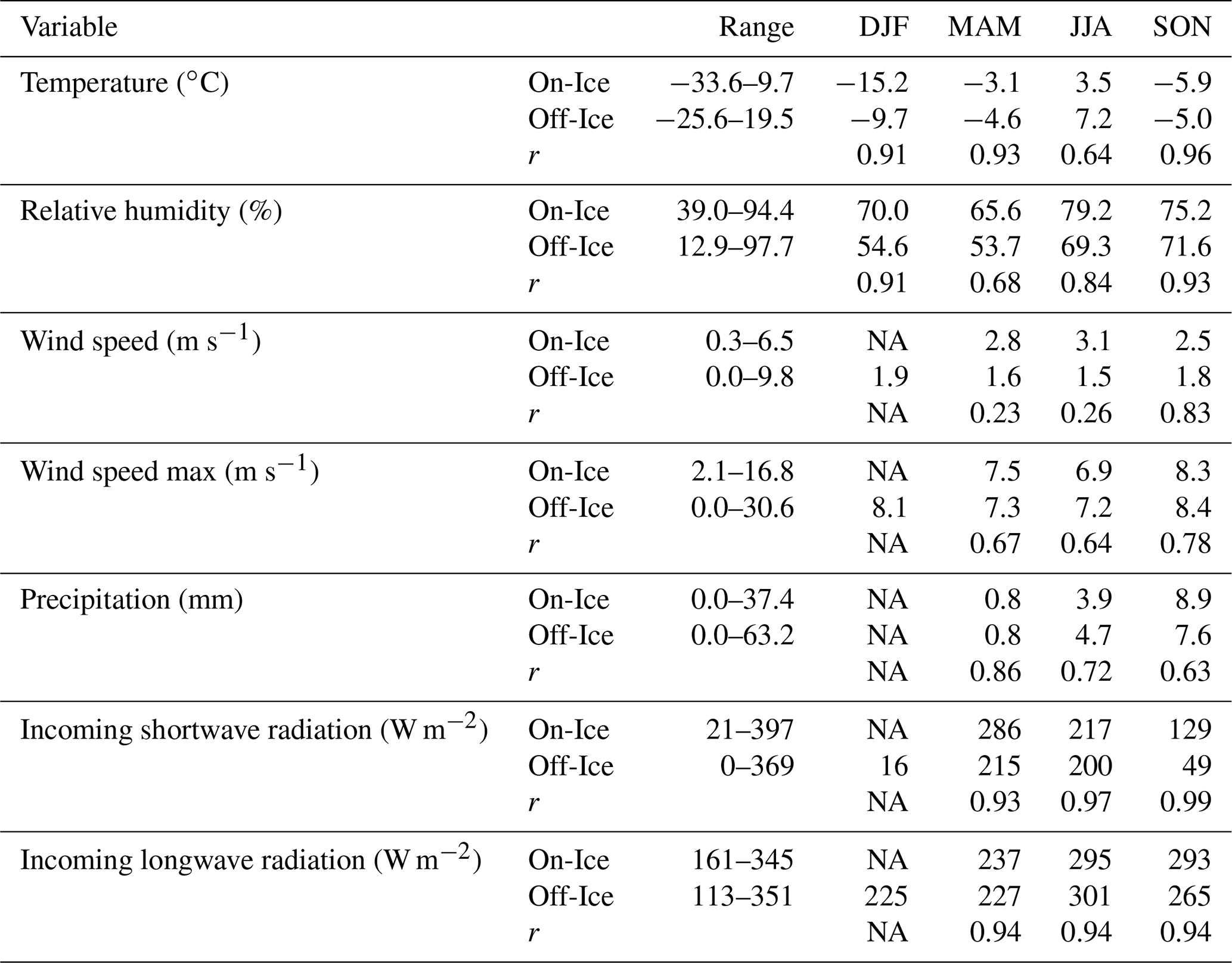
Table 2Seasonal means of meteorological variables for the On-Ice and Off-Ice stations based on data between 18 April 2013 and 6 September 2014. All data are for times when both stations were operating, so these data do not represent full season averages. Data were excluded from the period when the On-Ice station was buried by snow: 18 January to 22 April 2014. Correlations for precipitation excluded days when both stations had no precipitation. NA denotes no data were available.
3.1.2 Meteorological data
The daily meteorological data for both the On-Ice and Off-Ice station are shown in Fig. 4, and seasonally averaged correlation coefficients between the two station's daily data are given in Table 2. Air temperatures at each station were significantly more variable in winter than in summer due to frequent winter weather systems. Both station's daily temperatures correlated well in all seasons except summer (June–August), when temperatures at the On-Ice station exhibited considerably less day-to-day variability than the Off-Ice station. In addition, albeit 118 m lower in elevation, the On-Ice station's temperatures were more than 4 ∘C cooler than the Off-Ice station. These differences are attributed to the fixed glacier surface temperature of 0 ∘C during extended periods of glacier melting during summer. The cold glacier surface cooled the air above it. Though differences were not as pronounced, lower air temperatures at the On-Ice station were also observed during other seasons. This is due, in part, to the high albedo at the On-Ice station.
Relative humidity at the On-Ice station was typically higher than at the Off-Ice station, consistent with lower air temperatures and greater availability of moisture for evaporation over the glacier. The On-Ice station also displayed less day-to-day variability than at the Off-Ice station.
Daily mean wind speeds were typically higher at the On-Ice station than at the Off-Ice station, which can be attributed to the relatively smooth glacier surface, longer fetch, and summertime katabatic wind. The highest wind speeds occurred during winter with maximum wind gusts (3 s averages) up to 30.5 m s−1 (11 December 2013).
Vector-averaged daily wind directions were commonly in the down-glacier direction (65∘ On-Ice, 100∘ Off-Ice), consistent with a katabatic wind. In summer, the wind direction would often reverse during part of the day, causing the daily directions to be more variable.
Total precipitation at the Off-Ice station was slightly higher (9 %) than at the On-Ice station during the periods both stations were functional; however, direct comparison is difficult since the instrumental setup was different with no wind shield and installation higher above the surface at the On-Ice station.
Incoming solar radiation displayed pronounced seasonal variability consistent with the site's latitude close to the polar circle. Daily mean values varied between just 16 W m−2 in winter and approximately 400 W m−2 in summer. Cloudy days in summer are clearly discernible due to their lower shortwave radiation compared to neighboring sunny days. High correlation (r=0.97) between both daily time series indicates relatively homogeneous cloud conditions at those sites. A portion of the difference between the two stations may be due to topographic shading.
In both 2013 and 2014, daily albedo in May and June had peaks between 0.7 and 1, and by late July and August albedo fell to 0.2. The summer of 2013 featured a drop in albedo from 0.6 to 0.2 over 5 d starting 25 June 2013, indicating the transition of a snow-covered to a snow-free surface. In 2014, the same transition took 1 month starting 4 July 2014. We did not measure reflected shortwave radiation at the Off-Ice station, but we expect it to be significantly lower than the On-Ice station due to the low albedo of the rocky surface compared to the On-Ice glacier surface.
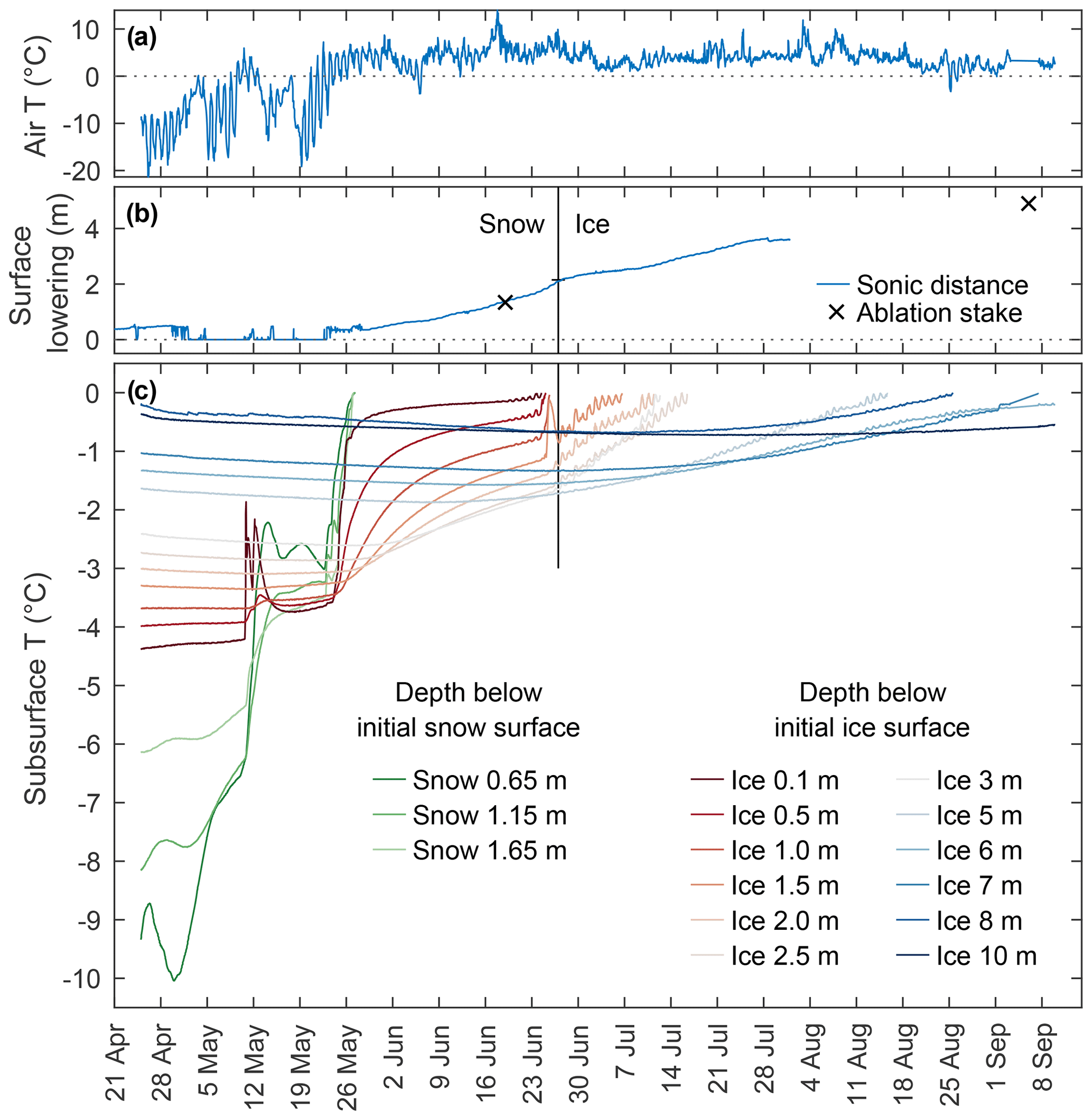
Figure 5Hourly ice and snow temperature (T) measurements from thermistors installed at depth in the snow and ice adjacent to the On-Ice weather station in 2013 (c). Panel (a) shows air temperature, and (b) shows cumulative surface lowering measured by the sonic ranger and ablation stakes. Initial thermistor depths are listed in the legend given in depth below the initial snow surface for the three snow thermistors and depth below the snow–ice surface interface for the 12 ice thermistors. The snow depth at installation on 19 April 2013 was 2.10 m. Note that the instrumentation depth becomes shallower as the glacier surface ablates during the melt season. The onset of large diurnal temperature fluctuations above 0 ∘C indicates that the thermistors have melted out and are affected by solar radiation. After a sensor exceeds 0 ∘C, we do not plot the remaining data.
Incoming longwave radiation, which mainly depends on the effective radiative temperature of the atmosphere, showed a slight seasonal cycle (Off-Ice station) with an amplitude of roughly 80 W m−2. Large daily variations superimposed on the seasonal cycle and negatively correlated with incoming solar radiation indicate variations in cloud cover. Incoming longwave radiation was well-correlated between the On-Ice and Off-Ice stations (r=0.94 for summer).
In both summers (2013 and 2014), outgoing longwave radiation increased through the spring to just below 320 W m−2 in mid-June and then plateaued through the end of August. Blackbody radiation from an object at 0 ∘C would be expected to be 316 W m−2, indicating that the effective radiative temperature of the ice surface and air between the surface and the sensor was just above 0 ∘C, and the surface was melting uninterruptedly for extended periods in summer.
Table 3Sensors used for the simple glacier and tundra weather stations. Glacier stations included only temperature and relative humidity while tundra stations also included precipitation and soil temperature measurements.

1 Shielded with a HOBO M-RSA Gill-type shield. 2 Shielded with a NovaLynx Alter-type rain gauge wind screen.
3.1.3 Snow and ice temperatures
The thermistor string we deployed in a hot-water-drilled borehole needed time to equilibrate to its surroundings after installation. We consider the thermistor ice temperature measurements to be reliable starting on 25 April 2013, about 8 d after installation. By that time, the 5 m deep thermistor temperatures were within 0.02 ∘C of the trend they held for the subsequent 4 weeks.
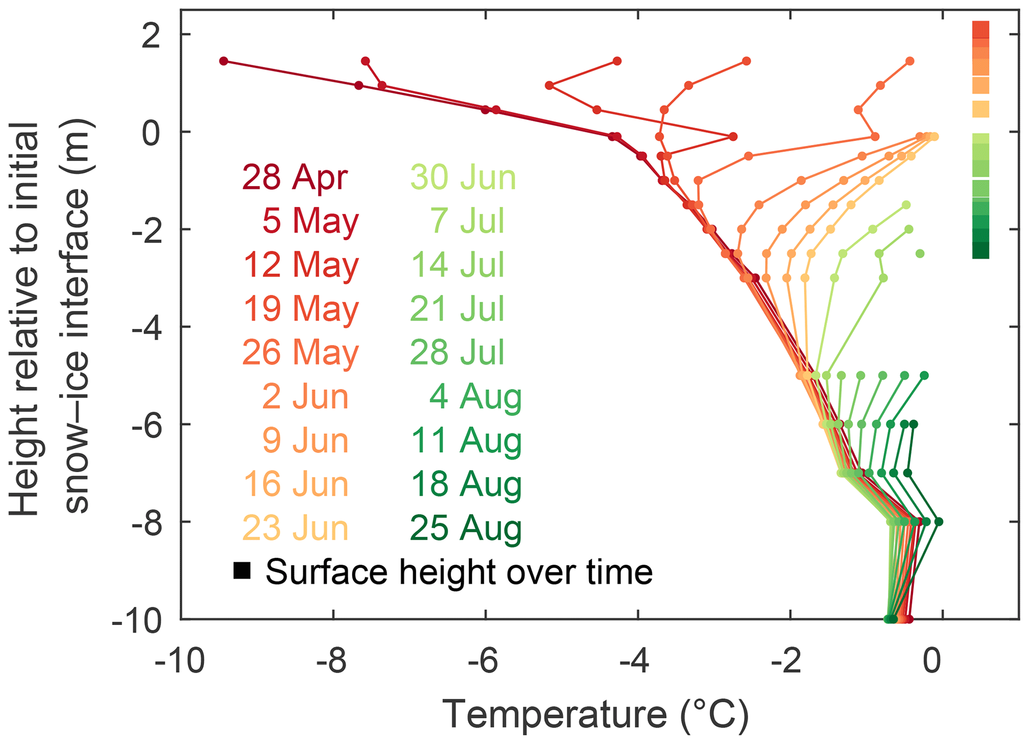
Figure 6Vertical profiles of temperature in the upper 10 m of the glacier at the On-Ice station in summer of 2013. After a sensor exceeds 0 ∘C, we do not plot the remaining data.
Temperatures within the upper 10 m of the glacier surface ranged from approximately −10 ∘C in the upper layers of snowpack in early May 2013 to close to the melting point of 0 ∘C at 10 m below the ice surface (Fig. 5c). As air temperatures rose, the subsurface temperatures of the upper layers increased but with a time lag that increased with depth (Figs. 5 and 6). When the air temperature rose above 0 ∘C, surface melt began to occur. As meltwater or rain percolated into the snowpack it refroze, causing abrupt temperature increases at the uppermost thermistors (e.g., 10 and 25 May 2013, Fig. 5). The glacier surface lowered with respect to the subsurface sensors by roughly 5 m between late April and early September 2013 as the melt season progressed (Fig. 5b). The three snow sensors and uppermost six ice sensors were exposed to the air sequentially during the summer melt season. On 24–25 June, the ice temperature sensors at 0.1, 0.5, 1, and 1.5 m below the snow–ice interface all experienced rapid warming to about 0 ∘C. The 1.5 m sensor then cooled back down to −0.85 ∘C. We interpret this to be another meltwater event but this time in the upper layers of glacier ice rather than the snowpack. It is difficult to know whether the event was representative of conditions in the glacier (i.e., water moving through cracks and along grain boundaries in the ice) or simply conditions along the thermistor cable. By 27 June, all 2.1 m of snow at the site had melted and the ice surface was exposed, as measured by the SR50 and confirmed with the time-lapse imagery. After 27 June, sensors at 2, 2.5, and 3 m depth exhibited diurnal temperature wiggles with an amplitude of up to 0.2 ∘C. By mid-July the diurnal wiggles appeared in the sensors at 5, 6, and 7 m depth too. Some of the ice temperature sensors at depths ⩾ 5 m recorded temperatures greater than 0 ∘C starting in late August 2013. These measurements are likely errors, perhaps due to faulty voltage sensor outputs. The data logger continued to record reasonable results for other variables.
3.2 Simple weather stations
3.2.1 Instrumentation
To supplement the multivariable weather stations described above and constrain the spatial patterns of temperature and precipitation within the basin, we installed 26 simple weather stations across the basin both on and off the glaciers (Fig. 1; Table A1). The 14 stations on or very near the glaciers (EF1, EF2, EF3, Mac1, Mac2, Mac3, Repeater HOBO, NWTrib1, Off-Ice HOBO, SU1, SU3, WF1, WFTranB, WF5; letters refer to glacier names) measured air temperature and relative humidity at a nominal height of 1.75 m above the glacier surface. We refer to these stations collectively as the “glacier” weather stations. The sensor mounts for the glacier stations were designed to maintain approximately the same sensor height relative to the glacier surface throughout the ablation season. This was accomplished by allowing the mount to slide down the ablation stake as the glacier surface melted (Fig. 3). The other 12 simple weather stations are referred to as the “tundra” stations. The typical tundra station measured temperature, relative humidity, rainfall, and soil temperature at 10 cm and 1 m depths. Simple weather station instruments are listed in Table 3.
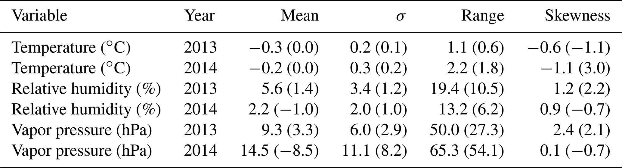
Table 4Statistics of air temperature and humidity sensor calibration. Eight HOBO sensors were calibrated in 2013 (5–8 April) and 14 sensors in 2014 (15–18 April). For each year the differences in hourly means between each HOBO station and a reference station were calculated; then the differences from all stations were concatenated before calculating the mean, standard deviation, range, and skewness of the distribution. Two reference stations were used: a Rotronic HygroClip2 temperature–RH probe measured by a Campbell data logger and an arbitrarily chosen HOBO station (data in parentheses).
Temperature and relative humidity were recorded every 10, 15, 30 min (most stations), or 60 min, depending on the station. Each station's data were then averaged in post-processing to hourly and daily values. Hourly and daily precipitation sums were calculated for each tip of the rain gauge tipping bucket.
3.2.2 Sensor calibration
To ensure the validity of data collected from many individual sensors scattered across our study area, we set them up side by side before deploying them to the field. Eight factory-calibrated HOBO temperature and relative humidity sensors were co-located with a factory-calibrated Rotronic sensor connected to a Campbell data logger in April 2013 in Fairbanks, Alaska. To avoid errors due to direct solar radiation, the sensors were installed in an outside area shaded during most hours, in particular during midday. Another set of 14 HOBO sensors was calibrated at the same location in April 2014. Measurements were taken and logged every 5 min. Hourly averages were also logged.
Temperatures during the 2013 calibration period ranged from −22 to −5 ∘C and from −15 to +10 ∘C in 2014 (Fig. 7). The temperature offset of hourly-mean HOBO sensors relative to an arbitrarily chosen reference HOBO station was typically within ±0.1 ∘C and rarely beyond ±0.3 ∘C. Over both periods, the temperature offset had a mean of 0.02 ∘C and a standard deviation of 0.07 ∘C (Table 4).
Compared to the Campbell–Rotronic sensor, HOBO temperatures were lower by 0.2–0.3 ∘C on average (Table 4), but differences exhibited a diurnal cycle with temperatures more than 1 ∘C lower during midday in many cases (Fig. 7). The 5 min data showed that the response time of the HOBO sensors was slower than that of the Campbell sensors, but this can not explain the differences in hourly or daily means (Fig. 8). The correlation coefficient between hourly values of temperature from the Rotronic sensor and HOBO sensors was 1.0.
The lack of a consistent pattern in these comparisons (Fig. 7) prevented us from adjusting the HOBO temperature data to match the Campbell data. The high correlation and low temperature offsets (Fig. 8) among sensors gave us confidence that using HOBO stations to assess temperature patterns across the basin was valid.
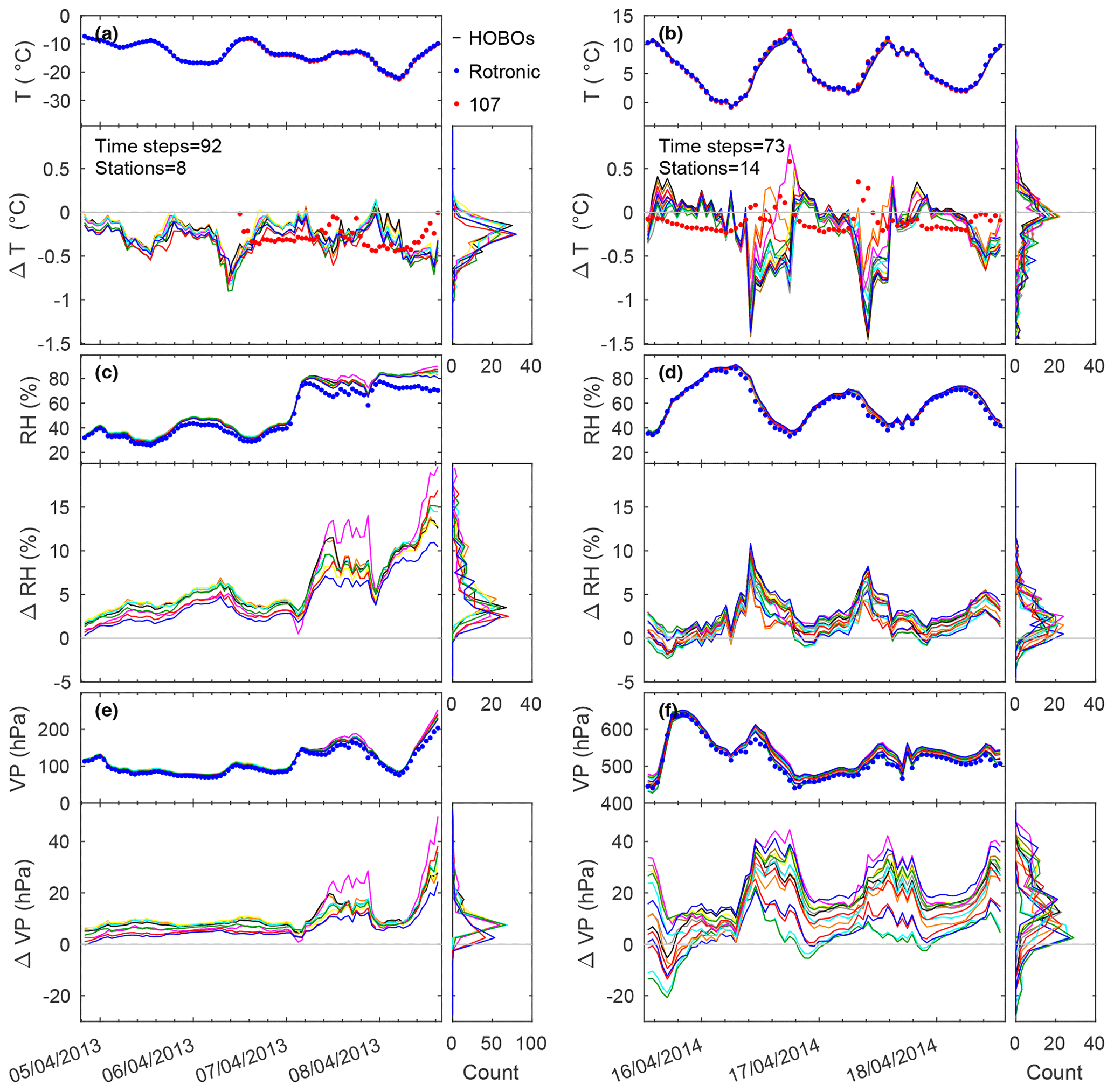
Figure 7Time series of hourly air temperature T (a, b), relative humidity RH (c, d), and derived vapor pressure VP (e, f) of eight HOBO sensors during the calibration period in 2013 (a, c, e) and 14 sensors in 2014 (b, d, f) and their differences to the Rotronic reference sensor. Each colored line represents a HOBO sensor, blue dots are for the reference Rotronic sensor, and red dots are for a Campbell 107 temperature probe. Also shown is the count of differences between HOBO and reference values in bins of 0.1 ∘C, 1 %, and 5 hPa.
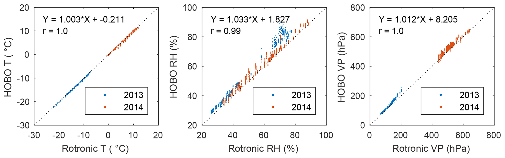
Figure 8Hourly-averaged data from all HOBO sensors compared to the Rotronic sensor for the calibration periods in 2013 (5–8 April) and 2014 (15–18 April). Equations of the best-fit lines and correlation coefficients are listed in each panel.
Measured relative humidity ranged from approximately 25 % to 90 % during the April 2013 calibration period and about 20 % to 90 % in April 2014 (Fig. 7). HOBO sensors generally recorded higher relative humidity compared to the Rotronic sensor (Table 4). The offset in temperature (HOBO was colder than Campbell) explains part of that difference, though absolute humidity calculations show that the HOBO sensors registered higher total moisture content for both the cold (2013) calibration period and the warmer one (2014). Relative humidity values from the HOBO sensors were well-correlated (r=0.99) with those from the Rotronic sensor (Fig. 8). Again, this gave us confidence that we could use our data to assess humidity variations across the basin.
In mid-April 2014, a laboratory calibration of the tundra station precipitation tipping-bucket gauges revealed an intermittent instrument signal problem (Wolken et al., 2015). Single tips in the rain gauge were being recorded as two tips on the data logger; thus the recorded precipitation amount appeared to be twice as much as the actual rainfall amount. In the field data, all HOBO stations recorded some of these double tips. A few tundra stations recorded up to 10 % double tips (Kosina Creek Upper, Kosina Creek Lower, and Windy Lower). Precipitation rates that could cause two tips within 2 s (360 mm h−1) far exceed the actual precipitation rates observed in the basin. To correct this data problem, for every pair of tips that occurred within 2 s, we zeroed out the second tip. The analysis done in this paper uses the corrected rainfall data.
We looked for similar double tips in the On-Ice and Off-Ice station data but did not find any. The HOBO and Campbell sensors use the same internal electronics to detect tips, so we surmise that the Campbell logger is filtering out any double tips before recording the data.
3.2.3 Spatiotemporal variability of air temperature, humidity, and precipitation
Time series of daily air temperature, humidity, and precipitation of all stations (On-Ice, Off-Ice, and tundra stations) are shown in Fig. 9.
Cumulative measured precipitation amounts for the summers 2012, 2013, and 2014 varied significantly across the domain, while the timing of events was generally consistent among the stations (Fig. 9). Precipitation amounts did not correlate significantly with elevation, slope, aspect, or location.
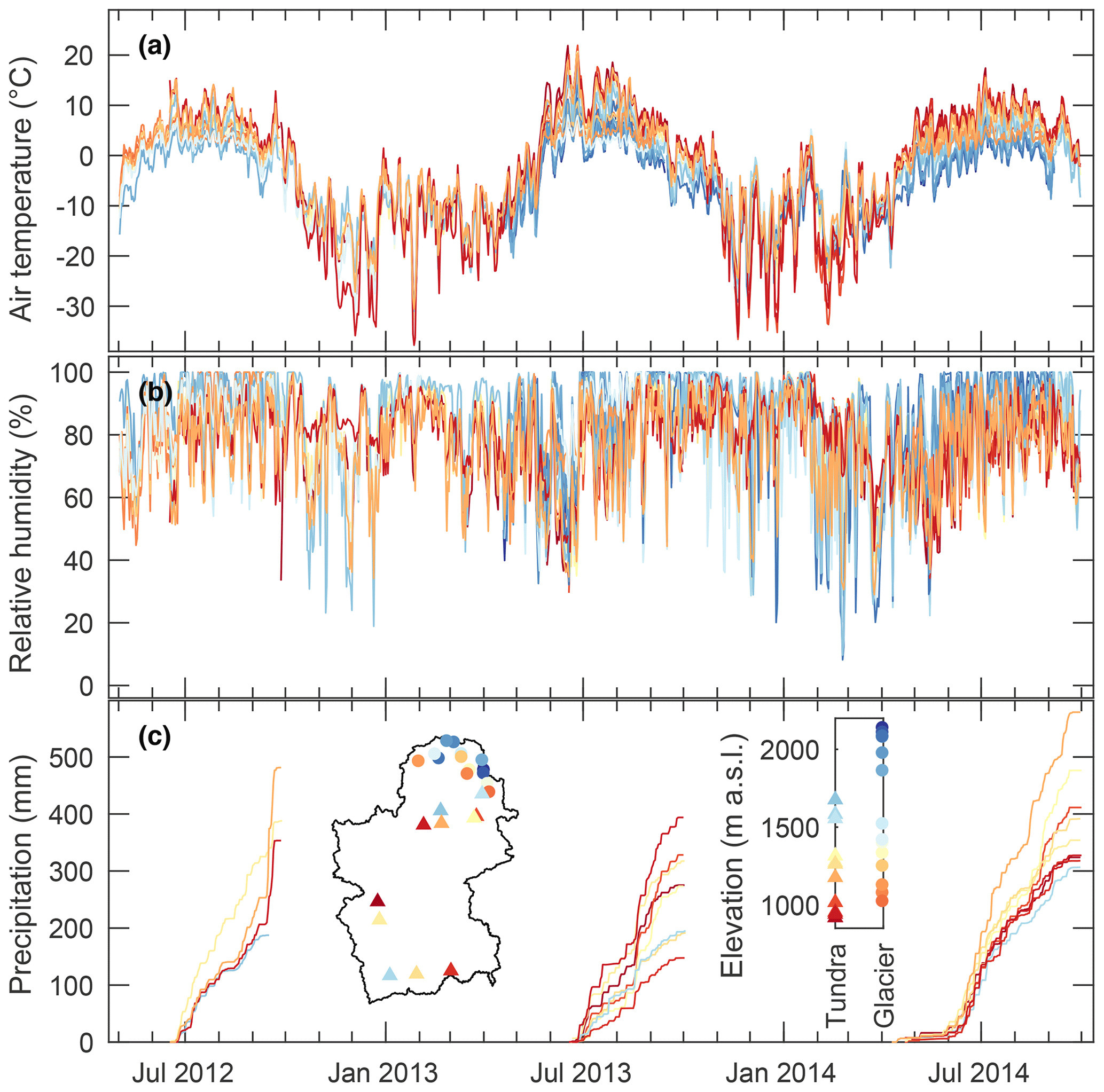
Figure 9Daily mean temperature (a), relative humidity (b), and cumulative precipitation (c) for the tundra and glacier stations. Data are colored by station elevation (inset graph). The inset map shows station locations.
Air temperatures at all sites showed similar seasonal variations, but as expected temperatures varied with elevation. Figure 10 shows largely linear trends of monthly mean temperature with cold temperatures at high elevations in summer of 2013 and 2014. Environmental temperature lapse rates showed a larger temperature gradient for the tundra stations compared to the glacier stations. In summer, when air temperatures were above freezing, the ice surface cooled the air over the glacier. This cold air descended due to its greater density than the air around it, setting up a katabatic flow. Continued cooling from the glacier partially offset adiabatic warming as the air descended and led to the lower temperature gradient at the glacier stations.

Figure 10Monthly air temperature profiles from simple weather stations on the glaciers and on the tundra. Environmental lapse rates (∘C km−1) were calculated by linear regression between monthly average data and station elevations and are reported in the upper right of each subplot, along with the r value of the fit.
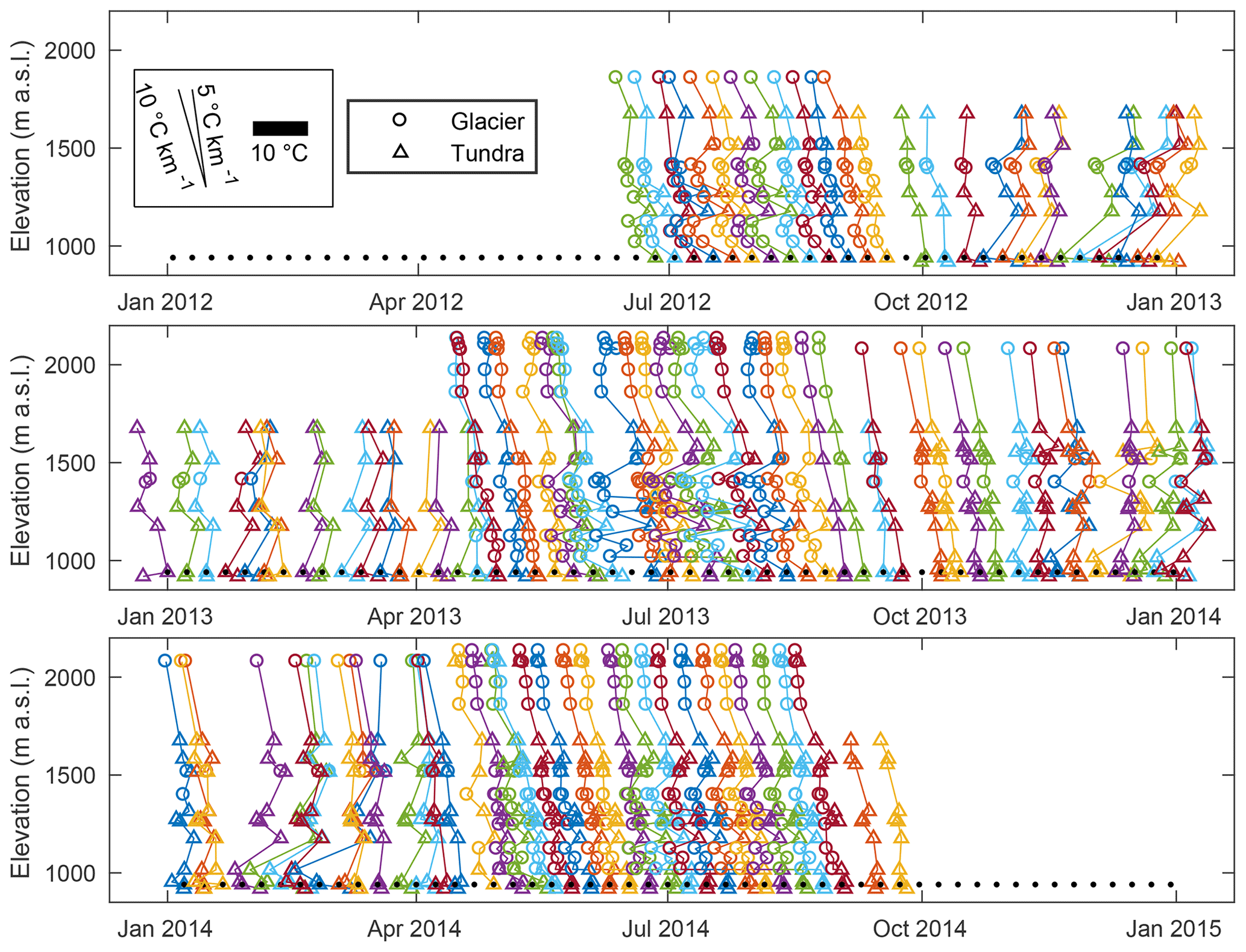
Figure 11Weekly air temperature profiles show the winter inversions and summer differences between glacier and tundra temperature. For each week, the reference station (Windy Creek Lower, 940 m a.s.l., triangles and black dots) was plotted on the horizontal axis according to the date. The other stations (triangles or circles) were plotted to the left or right of the reference station according to their temperature difference. Stations with significant data gaps in a week were not plotted. Many glacier stations were removed in winter due to snow.
Given the difficulty of calculating monthly lapse rates due to missing data (Fig. 10), we also calculated weekly average temperature and plotted it to illustrate the changing lapse rate with the seasons across the basin (Fig. 11). The summer glacier–tundra pattern transitioned back to a single lapse rate when the air temperature fell below 0 ∘C. Winter inversions (with warmer air at higher-elevation stations) are common, such as in January 2013 and January 2014. The glacier station at 1400 m a.s.l. was buried by snow for part of each winter and therefore stands out as a warm outlier during those times. Springtime lapse rates are the most distinct – most stations fall along the best-fit gradient.
3.3 Trends
Our field measurements did not cover enough time to establish long-term trends of temperature or precipitation. For context, we evaluated nearby stations with long-term records from the National Climatic Data Center. The best correlations with our On-Ice station, for temperature and precipitation, came from Talkeetna Airport. The Talkeetna station was 197 km southwest of the On-Ice station and almost 1300 m lower, at 107 m a.s.l. Summer temperatures at Talkeetna Airport in 2012–2014 were 1.1 ∘C warmer than 1981–1983. Annual temperatures were 0.5 ∘C warmer in the recent period. Precipitation was variable year to year but showed little trend. Annual precipitation for the 3-year interval in the 1980s averaged 746 mm, and in the 2010s it averaged 747 mm.
Glacier mass changes were determined from in situ point observations in spring and fall of each year, snow radar measurements in spring, and continuous measurements of relative surface elevation change at the On-Ice Weather station.
4.1 In situ point mass balance measurements and derived glacier-wide balances
Winter, summer, and annual mass balances were measured at 27 to 29 locations spread across the five largest glaciers, West Fork, Susitna, East Fork, Maclaren, and Eureka (Fig. 1) using the glaciological method (Cuffey and Paterson, 2010). The stake distribution was designed to reoccupy the approximate stake positions used in the Clarke et al. (1985) study covering 1981–1983 and to sample the elevation range of each glacier. Most measurement sites followed the centerline of glaciers. We performed measurements for three mass balance years: 2012, 2013, and 2014, where a mass balance year refers to October to the following September. For example, year 2012 refers to October 2011 to September 2012. Winter snow accumulation on glaciers was estimated at each stake by snow probing and/or snow pit measurements in late April of each year. The amount of snow and ice that melted each summer was measured at each stake in early September.
The most negative annual point balance among the measured glaciers was almost −6 m w.e. (2013 at 1100 m a.s.l. on East Fork Glacier), while the most positive was nearly 2 m w.e. (2014 at 2000 m a.s.l. on Susitna Glacier). Figure 12 indicates a strong elevation dependence of all point balances. The equilibrium line altitude for the region was about 1730 m a.s.l. in 2012 and 1960 m a.s.l. in 2013, as estimated from the zero crossing of the best-fit line to the mass balance profile data (Fig. 12). With a large fraction of the glacier at higher elevations (Fig. 12), this corresponds to an accumulation area ratio of 0.58 for 2012 and 0.34 for 2013. Wastlhuber et al. (2017) used Landsat imagery to derive equilibrium line altitudes for the set of five large glaciers of about 1675 m a.s.l. for 2012 and 1800 m a.s.l. for 2013. Their 2012 value matches ours within uncertainties, but our 2013 value is significantly higher, indicating the surface mass balance might not have been accurately estimated from satellite data or the best-fit line might be too sensitive to data from lower elevations.

Figure 12Annual point mass balances measured with the glaciological method on West Fork, Susitna, East Fork, Maclaren, and Eureka glaciers. The apparent outlier in 2012 (−1.4 m w.e. at 908 m a.s.l.) was due to debris cover at the site. The hypsometry of all 127 glaciers in the Alaska Range portion of the Susitna basin is also shown in 50 m elevation bands. The hypsometry comes from the Randolph Glacier Inventory (Pfeffer et al., 2014), which used glacier outlines from 2009 and elevation from airborne interferometry (http://ifsar.gina.alaska.edu, last access: 6 December 2018) collected in summer 2010.
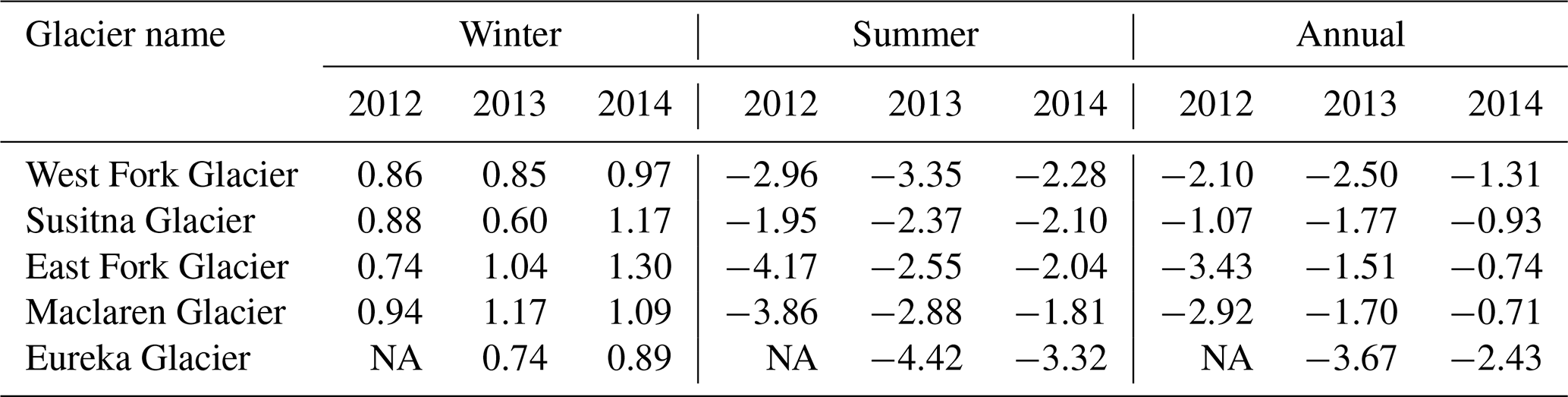
The point mass balance measurements were used to compute the glacier-wide winter, summer, and annual mass balance for each of the five glaciers for the mass balance years 2012, 2013, and 2014. First, we linearly interpolated the mass balance measurements across elevations to get a continuous mass balance profile for each glacier for each year. Glacier elevations above and below the measurement range were assigned the mass balance value of their nearest neighbor. The mass balance profiles were distributed to the entire glacier area based on the glacier hypsometry (50 m elevation bins). Glacier-wide mass balance estimates were then calculated by summing the distributed mass balance over the whole glacier. Annual balance was calculated from the sum of winter and summer balance (Table 5). Winter glacier-wide balances ranged from 0.74 to 1.3 m w.e. Glacier-wide summer balances ranged from −4.42 to −1.81 m w.e. The summer balance in 2014 was less negative than in 2012 and 2013. Annual balances ranged from −0.71 to −3.67 m w.e. The glacier-wide annual balance was negative for all years and all glaciers, indicating that the summer mass loss was greater than the winter accumulation. The annual balance in 2014 was less negative than in 2012 and 2013.
4.2 Glacier mass balance: comparison to 1980s data
Mass balance on the glaciers changed substantially from 1981–1983 to 2012–2014 (Fig. 12). Glaciers in the early 1980s generally had more positive or less negative mass balance than the early 2010s across all elevations (Fig. 12). The year 2013 had the most negative mass balance of the 6 years measured and the highest equilibrium line.
Glacier-wide summer mass balances became more negative between the 1980s ( m water equivalent, mean ± SD of four glaciers) and 2010s ( m w.e. mean ± SD of the same four glaciers with stakes in approximately the same locations). In contrast, winter balance was similar between the 1980s (0.88±0.22 m w.e.) and 2010s (0.97±0.20 m w.e.). Therefore, lower annual balance in the latter period ( m w.e.) compared to the former period (0.04±0.25 m w.e.) was driven by the more negative summer balance. These mass balance patterns are consistent with the warming temperatures and relatively stable precipitation measured at Talkeetna Airport.
Table 5Glacier-wide winter, summer, and annual mass balance (m w.e.) on the five largest glaciers in the Upper Susitna basin, 2012–2014. Mass balances were measured during site visits in the following date ranges: 26 April to 2 May 2012, 26–28 September, 15–21 April, 6–15 September 2013, 22–27 April, and 7–9 September 2014. Exact dates for individual stake measurements are listed in the data set. NA denotes no data were available.
4.3 Radar-derived accumulation in glacierized terrain
Unlike ablation, which tends to be spatially coherent and well-correlated with elevation, snow accumulation typically shows pronounced small-scale variability, making it difficult to accurately measure and model (Sold et al., 2013). This is especially true in complex terrain, where topography and meteorological processes vary over short distances (McGrath et al., 2015).
To evaluate how representative our stake measurements of snow accumulation were of the broader glacier area, we conducted helicopter-borne ground-penetrating radar (GPR) common-offset surveys of snow accumulation over the five main glaciers and glacier foreland areas in the Upper Susitna basin following Gusmeroli et al. (2014) (Fig. 13). We then used in situ measurements of snow density to calculate end-of-winter snow water equivalent (SWE) for each year during the period of 2012–2014. Radar-derived estimates of winter snow accumulation illustrate the high spatial variability across the elevation range of each glacier and from one glacier to another across the basin (Fig. 13). Elevation is the dominant influence on SWE at the Upper Susitna basin scale, with snow accumulation on the glaciers at 2000 m measuring 2–4 times higher than that at 1000 m. Over short spatial scales in the ablation zone, surface roughness is responsible for high spatial variability in SWE. The end-of-summer glacier surface is rough due to streams, crevasses, melt ponds, and moraine material. The end-of-winter snow surface tends to be relatively smooth compared to the summer surface but can also have wind-derived roughness features that contribute to the variability in SWE over small distances.
There is good correspondence between the radar measurements and the traditional method (Fig. 13). A few points at high elevation where the discrepancies are largest might be explained by a misinterpretation of the location of the previous summer surface, either by manual measurement (probe) of a shallow ice layer or by selection of a deeper firn layer in the radar data.
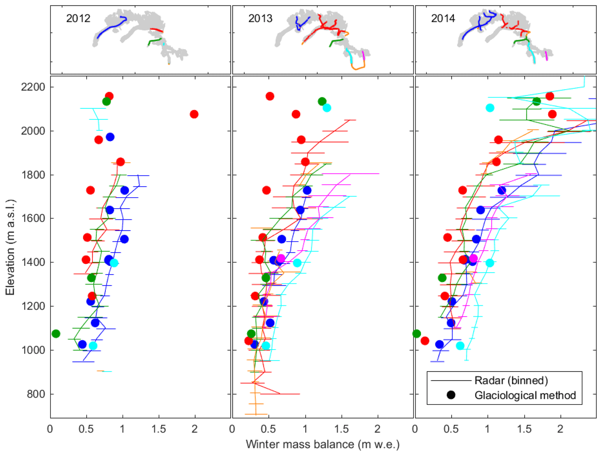
Figure 13Winter mass balance profiles in 2012–2014 derived from point mass balance measurements (filled symbols) and from helicopter-based radar data. Horizontal lines represent mean ± SD over 50 m elevation bands).
4.4 Continuous point mass balance measurements
Adjacent to the West Fork Glacier weather station (1398 m a.s.l.) we installed an acoustic distance sensor and a Wingscapes time-lapse camera to measure snow accumulation and melt with high temporal resolution. The distance sensor was fixed vertically by mounting it on a pole drilled a few meters into the glacier, allowing the distance measured from the sensor to the surface to be directly related to melt or accumulation. The time-lapse camera was mounted to the On-Ice weather station and maintained a fixed height above the glacier surface. It took a picture facing the distance sensor every hour for the summer of 2013 and 2014.
Early in the 2013 record (16 April–28 May), the distance sensor was repeatedly covered by fresh snow accumulation, giving inconsistent readings (Fig. 14). From 28 May through 1 August 2013 the sensor gave reliable data and the measured net surface lowering due to surface mass balance was 3.3 m. After 1 August 2013, the sensor's mounting pole began to tip over and give meaningless readings. The tilt was observed in the time-lapse imagery (sensor absent from 26 August 2013 image in Fig. 15). There was very little summer snowfall in 2013. There was a distinct increase in measurement noise after the transition from snow to ice. This was likely caused when the acoustic signal bounced off different elements of the rough ice surface in successive measurements. The height change rate while the surface was snow-covered (28 May–25 June) was 0.053 m d−1. The net depth of snow lost at the sonic distance sensor site was 1.97 m (17 April–30 June), which is comparable to the 2.15 m snow depth measured in a snow pit about 6 m away on 14 April 2013 (Fig. 5). The ice surface lowered at a rate of 0.043 m d−1 (30 June–1 August).
In 2014, the distance sensor gave good readings from 26 April to 1 September when the sensor was removed after a 2 d snowstorm. The 2014 measured net surface lowering from the last significant spring snowfall (28 April) to the first fall snowfall (1 September) was 3.8 m; summer snowstorms added 0.86 m of snow to the glacier, which also melted away, for a total summer melt of 4.7 m. As in 2013, the 2014 data became noisier as the surface transitioned from snow to ice. The snow-covered surface lowered at a rate of 0.037 m d−1 (28 April–3 July) and the ice surface lowered at a rate of 0.030 m d−1 (3 August–1 September). Although the rate of surface lowering is larger for the snow surface than the ice surface, the rate of mass change is lower due to lower density. To calculate ablation from the observed distance change, we used a density of 350 kg m−3, based on the average of five snow density measurements at the site. This leads to an average melt rate of 0.016 m w.e. d−1 for the summer of 2013 and 0.012 m w.e. d−1 for 2014.
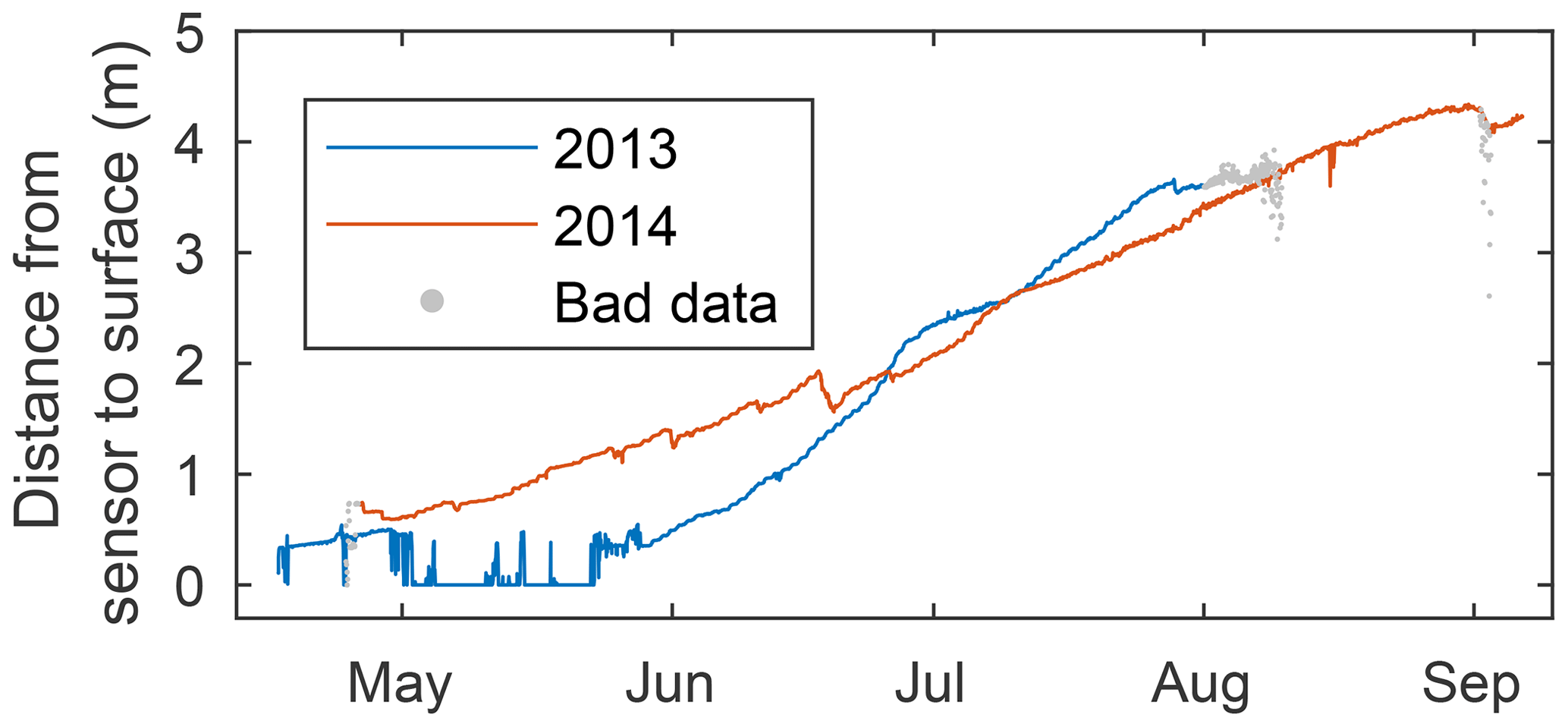
Figure 14Distance from the acoustic sensor to the snow or ice surface. Increasing distance is a result of snow or ice melt and snow settling. Decreasing distance is due to snow accumulation. In early August 2013, the sensor's mounting pole began to tip over and give bad readings. On 1–2 September 2014, 18 cm of snow accumulation was recorded, consistent with observations during a site visit. The sensor pinged off falling snow, so some points in that window are labeled as bad data.
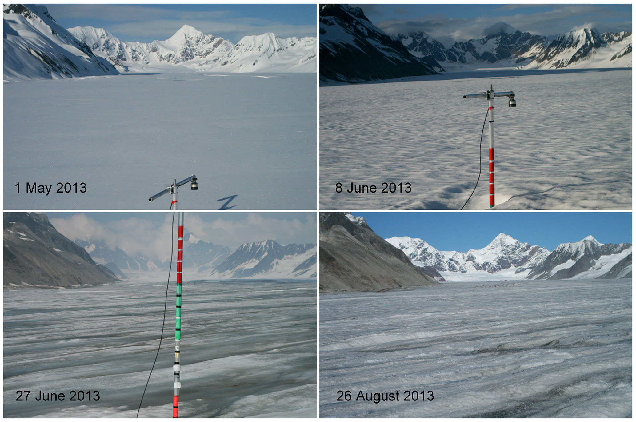
Figure 15Photos from the time-lapse camera on West Fork Glacier show surface conditions: smooth fresh snow (1 May 2013), aged snow with rougher surface (8 June 2013), recently exposed bare ice with some water-saturated snow (27 June 2013), aged ice surface (26 August 2013).
5.1 Field measurements of snow in spring 2012 and 2014
In situ snow measurements were made with a double sampling method (Rovansek et al., 1993) in non-glacierized settings (forest and tundra, see Fig. 1 for locations). At each site, three to five snow cores capturing the entire snowpack were extracted and weighed to calculate snow density. In 2012 we used an Adirondack snow tube and in 2014 a SnowHydro snow tube. A larger number (∼ 50) of snow depth measurements were also taken to improve the statistical properties of the sample. Snow water equivalent was calculated by multiplying the average snow depth with the average snow density. The sites were reached by helicopter (4 April 2012 and 22–28 April 2014) and via snow machine (8–12 April 2014). No measurements were obtained in 2013. The compiled measurements are presented in Table 6.
Table 6Spring snow depth and density measurements in non-glacierized terrain, April 2012, early April 2014, and late April 2014. Snow depths were averaged from about 50 measurements in the vicinity of each site. Density was averaged from three to five sites. The northing and easting are in the UTM Zone 6N.
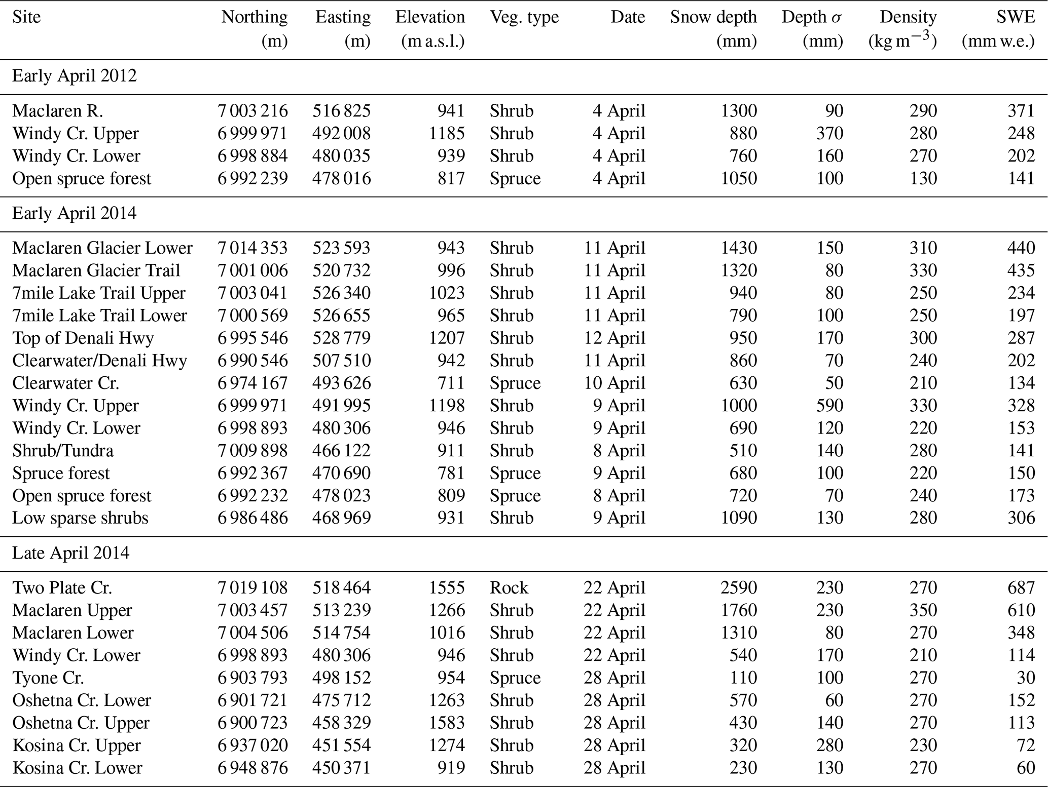
The field measurements showed variations in SWE according to elevation, region, and vegetation type but with the small number of sites, definitive statistics were not feasible. The SWE measurements illustrated a general increase with elevation in 2014, which became more significant in late April. Basin-wide SWE data distinguished three major regions (Maclaren, Clearwater and Talkeetna), where the Maclaren sites represented the highest SWE and the Talkeetna region the lowest. Within each region, the SWE data generally showed a strong increase with elevation. Among the two main vegetation types, shrubs presented larger SWE than the spruce locations (Table 6).
Lower Windy Creek was the only site where we collected SWE data more than once in a year. About 40 mm of SWE (25 %) was lost due to melt of the end-of-winter snowpack between 9 April and 22 April 2014 (Table 6).
5.2 Snow depth in non-glacierized terrain: comparison to 1980s data
A total of 165 snow depth measurements, at 16 locations in both glacierized and non-glacierized terrain, were collected in 1981 and 1982 by R&M Consultants (1982). Direct comparisons to our data are hampered by differing measurement locations and dates, though the 1980s generally had larger snow depths.
6.1 Soil pit characterization
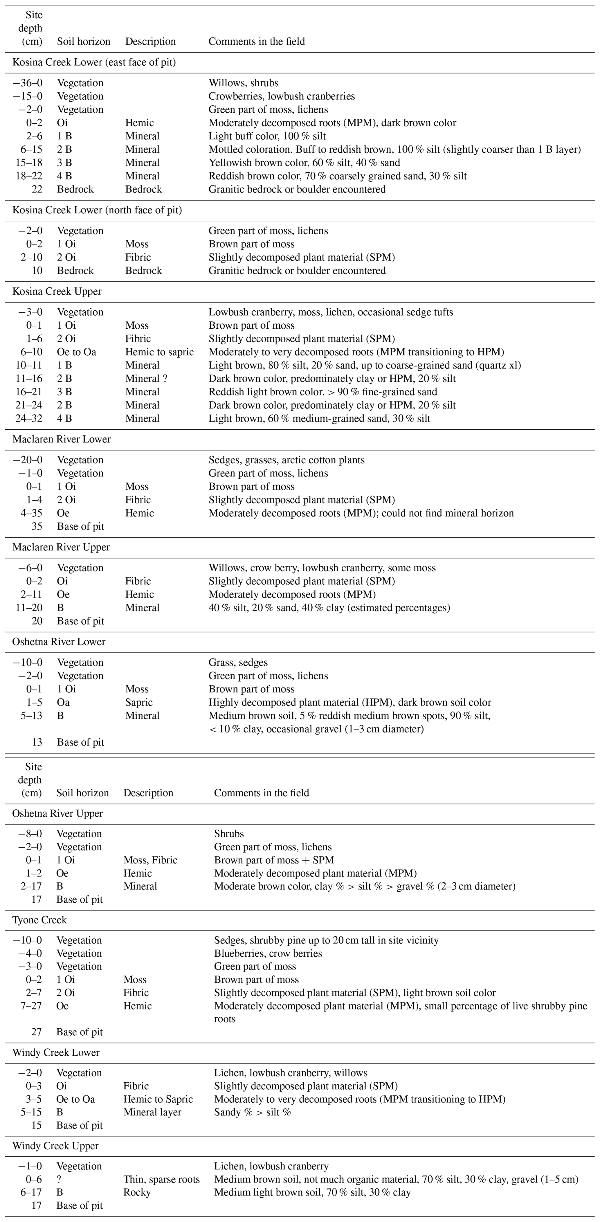
At each of nine tundra sites, we dug a soil pit from the surface down to the top of the mineral soil between 1 and 3 October 2013 (see Figs. 1, 16). We recorded the type of vegetation growing in the soil, visual characteristics of each soil horizon, as well as our estimation of the soil texture (Table A2). Two sites were too rocky to dig a pit (Two Plate Creek and Valdez Creek). The thinnest soils were generally observed at high-elevation sites. The thickest organic-rich soils were observed in low-slope low-elevation environments at Tyone Creek and Maclaren Lower. Though we did not do a detailed texture analysis on the soils, our observations of soil texture, organic content, and drainage characteristics generally matched up with the State Soil Geographic (STATSGO) soil map (https://datagateway.nrcs.usda.gov/, last access: 6 December 2018).
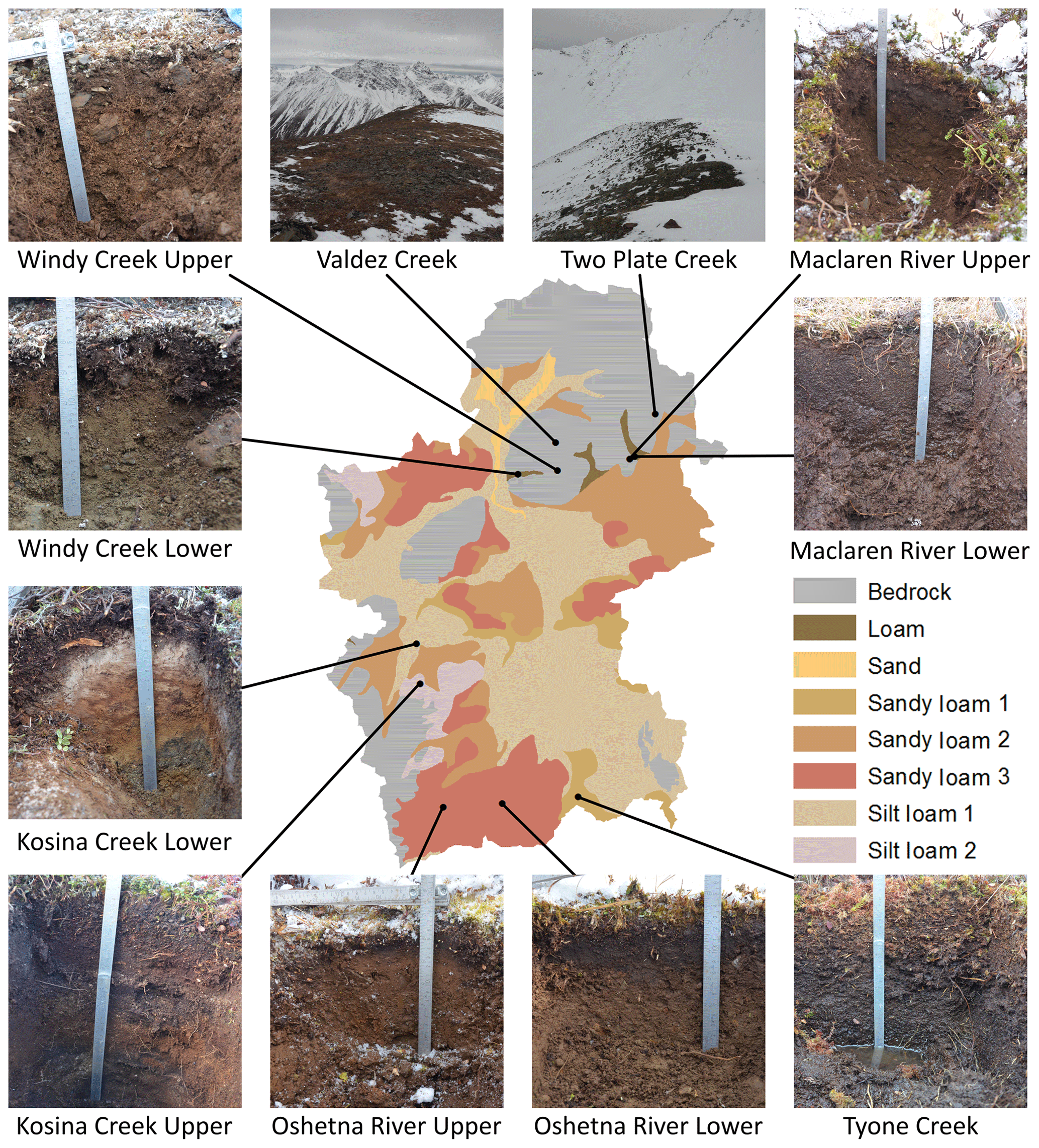
Figure 16Photos of shallow soil pits. The map shows STATSGO soil type boundaries and pit locations. The ruler in each photo is 1.5 cm wide. Pit depths range from about 10 to 35 cm.
6.2 Soil temperatures
Understanding the distribution of permafrost and seasonally frozen ground across the basin is important for modeling of water moving across the landscape. At each of the simple tundra weather stations installed over soil, we deployed soil temperature sensors at two depths below the surface (Fig. 17). Shallow sensors (10 cm depth) were deployed into the side of the soil pits described above and then the pits were back-filled. By pushing the sensors into the undisturbed soil on the side of the pit, we hope to minimize any temperature errors due to disturbance. We did not quantify the effects of disturbance on temperature, though we expect them to be small compared to the large temperature changes observed over the record. Deep sensors were deployed at the bottom of a 2.5 cm wide hole drilled into the ground. Disturbance of the soil around the deep sensors may affect temperature too, but we tried to minimize that by using the smallest drill we could. At some locations, the drill ran into rocks and was not able to reach the desired 1 m depth.
Broad patterns that we observed in the data include no permafrost in the upper layers of soil at the sites we sampled, although it may persist in deeper layers. The annual range of temperature at the shallow soil sensors is less than the air temperature range, and the day-to-day variability is damped too. The temperature cycles at the deep sensors (between 25 cm and 1 m depth, depending on the station) are even more damped than the shallow sensors.
Soil temperature at three sites (Tyone Creek, Maclaren Lower, and Maclaren Upper) was nearly constant through the winter at or just above 0 ∘C. At Tyone Creek and Maclaren Lower the ground surface was boggy and we observed liquid water seeping into our soil pits less than an hour after digging them (Fig. 16), indicating that water flow through the upper unfrozen layer may have contributed to the nearly constant soil temperatures. Soils at Windy Creek Upper and Kosina Creek Upper get colder than the other stations in the winter due to the rocky soil and relatively high elevation of those two sites.
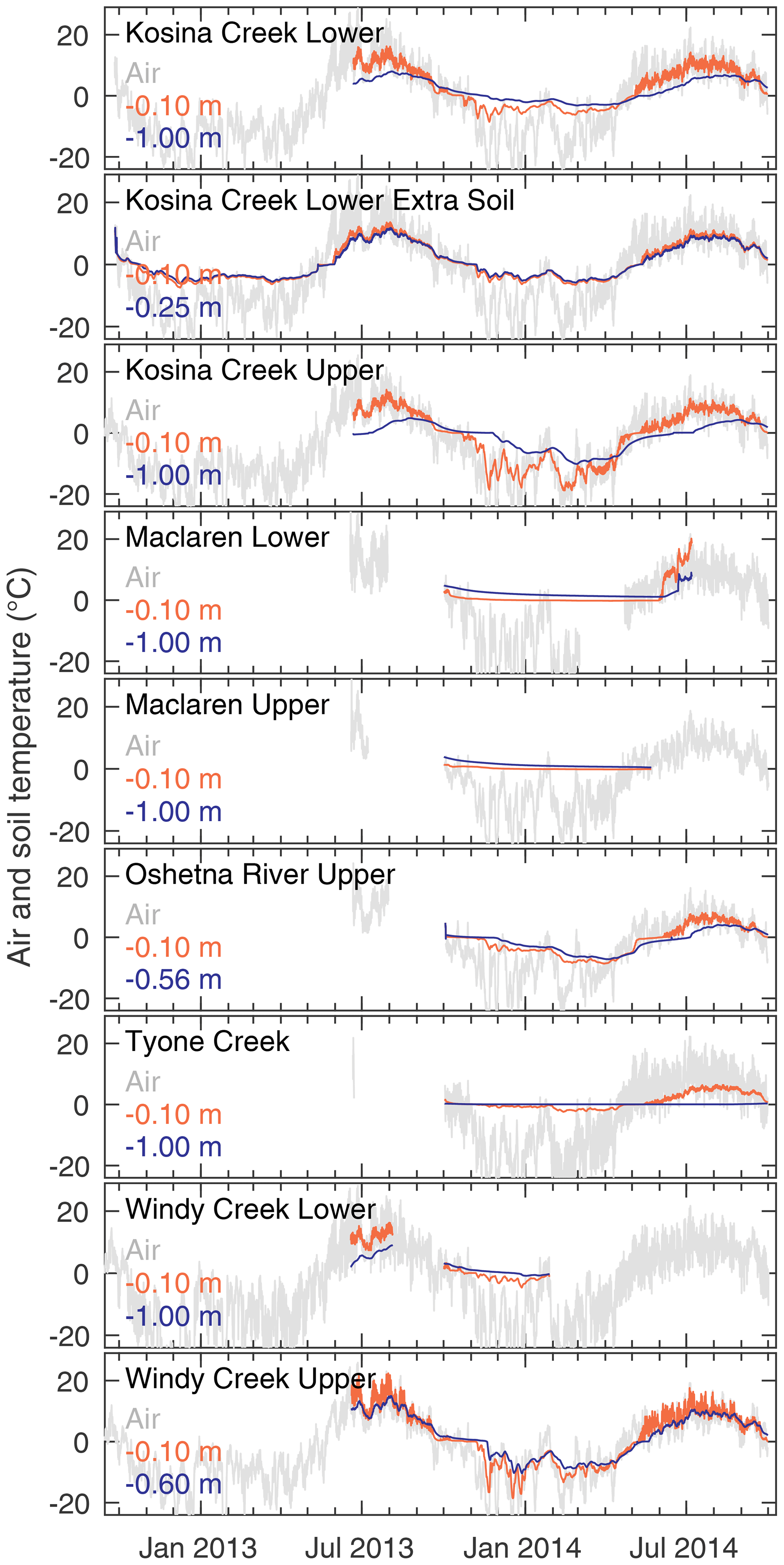
Figure 17Hourly soil temperatures at depth below the soil surface for all sites with soil data and air temperatures from each site's simple AWS. Each panel lists the depth of the soil temperature probes.
Figure 18 shows an example of summertime soil temperature fluctuations from the Windy Creek Upper station. Daily mean air and soil temperatures were all above 10 ∘C. The shallow soil (0.1 m depth) at this rocky site heated up even more than the air each day, particularly when it was sunny. The diurnal cycle was smaller in the shallow soil than in the air, and the deep soil (60 cm depth) showed only a very subtle diurnal cycle.
The middle panel of Fig. 18 shows a soil freezing event from fall 2013 at Kosina Creek Upper. Both the shallow (0.1 m depth) and deep (1 m depth) sensors start the period at about 4 ∘C and show a cooling trend over the interval due to heat loss to the atmosphere (sub-zero air temperatures). For the first day of the period, the shallow sensor exhibited a diurnal cycle of temperature with a magnitude of 2 ∘C compared to diurnal amplitude in air temperature of 10 ∘C. In combination with the cold air temperatures, it is likely that this site received snow on 17 September 2013. The Gulkana Airport National Climatic Data Center (NCDC) station to the east received 8 and 12 mm w.e. of snow on 17–18 September. The Matanuska station to the south received 4 and 8 mm w.e. of snow on 18–19 September. Interestingly, Talkeetna Airport to the west did not receive snow during this period. The diurnal cycle of temperature disappeared by 18 September. The soil continued to cool throughout the interval, reaching 0.2 ∘C at 0.1 m depth and 1.1 ∘C at 1 m depth by 7 October 2013.
Spring thaw of the upper 0.1 m of soil at Kosina Creek Upper occurred over a period of about 2 weeks in 2014. On 20 April the shallow soil temperature sensor recorded a mean temperature of −1.9 ∘C and a diurnal cycle variation of 2 ∘C while the air temperature diurnal amplitude was about 8 ∘C. As the air temperature warmed over the week of 27 April, the soil warmed to the freezing point and held steady until most of the soil had thawed. On 10 May, the shallow soil temperature exceeded 0 ∘C for the first time that year and thereafter resumed a diurnal cycle. The 1 m deep soils warmed from −6.3 to −1.7 ∘C over this interval.
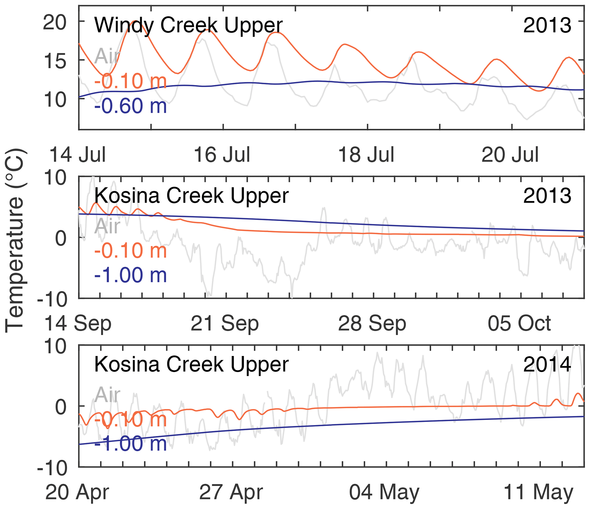
Figure 18Hourly soil temperatures at depth below the soil surface illustrating three time periods: diurnal fluctuations in summer, soil freezing in fall, soil thaw in spring. Air temperature data are repeated from Fig. 9 for context. Each panel lists the depth of the soil temperature probes.
Data are available at: https://doi.org/10.14509/30138 (Bliss et al., 2019).
Comprehensive observations of meteorology, snow cover, glacier mass change, and soil properties are important for assessing basin-wide changes and providing input to hydrological modeling. In this study we focused on the Upper Susitna watershed. Our measurements reoccupied many of the same sites used by an initial study of the region 30 years ago. The 1980s measurements in combination with those presented here provide a baseline for future studies in the area.
Summer air temperatures in 2012–2014 were 1.1 ∘C warmer than 1981–1983. Annual temperatures were 0.5 ∘C warmer in the recent period. We found lapse rates to be significantly lower over glacierized surfaces in summer than over non-glaciated areas. Our meteorological stations filled a large gap in observations (spatially and elevation). Through correlations with long-running NOAA sites, we can better estimate past conditions within the basin.
Glacier surface mass balance measurements showed that during the melt season the glaciers were losing mass more than 3 times more rapidly in 2012–2014 than in 1981–1983. Winter snow accumulation measured by traditional methods closely matched measurements gathered from a helicopter-borne snow radar. Annual glacier-wide mass balance went from being close to 0 m w.e. (balanced) in the 1980s to losing more than 1.5 m w.e. yr−1 in recent years. Snow depth in non-glacierized areas showed wide variability from site to site, reflecting complex deposition and redistribution patterns. Within local areas, higher elevations received more snow than lower elevations.
Our observations of soils in the basin generally match up with mapped soil descriptions. Soil temperature measurements revealed that none of the sites had permafrost in the upper 1 m of soil. Most sites froze in the winter, though three sites remained at the freezing point despite air temperatures of −20 ∘C.
The data sets described here provide new data in an extremely data-scarce region. The data are valuable as a baseline to assess future changes and will aid calibration and validation of hydrological, glaciological, and other environmental models.
Table A1Properties of meteorological stations referenced in this study. See Fig. 3 for example photos of our station types. The northing and easting are in UTM Zone 6N.
AB processed the data, performed all calculations and created all figures except Fig. 1 (GW), and wrote most of the manuscript. RH, GW, and EW contributed significantly to the development of the analyses and figures and the writing. AG processed the raw radar data. All authors but WH and JZ contributed to the fieldwork in the 2010s. WH provided information on the 1980s data. CA and AH contributed to some initial data analyses. RH, GW, AL, and JZ secured funding from the Alaska Energy Authority.
The authors declare that they have no conflict of interest.
This article is part of the special issue “Hydrometeorological data from mountain and alpine research catchments”. It does not belong to a conference.
The authors appreciate support and funding from the University of Alaska Fairbanks, Alaska Division of Geological and Geophysical Surveys, Alaska Energy Authority, and Colorado State University. Katreen Wikstrom Jones helped create Fig. 1. Joanna Young and A. Cody Beedlow were instrumental in launching the study.
This paper was edited by Kirsten Elger and reviewed by two anonymous referees.
Bahr, D. B., Meier, M. F., and Peckham, S. D.: The physical basis of glacier volume-area scaling, J. Geophys. Res., 102, 20355–20362, https://doi.org/10.1029/97JB01696, 1997. a
Bartholomaus, T. C., Anderson, R. S., and Anderson, S. P.: Response of glacier basal motion to transient water storage, Nat. Geosci., 1, 33–37, https://doi.org/10.1038/ngeo.2007.52, 2008. a
Bliss, A., Hock, R., and Radić, V.: Global response of glacier runoff to twenty-first century climate change, J. Geophys. Res.-Earth, 119, 717–730, 2014. a, b
Bliss, A., Hock, R., Wolken, G., Whorton, E., Aubry-Wake, C., Braun, J., Gusmeroli, A., Harrison, W., Hoffman, A., Liljedahl, A., and Zhang, J.: Glaciers and climate of the upper Susitna Basin, Alaska; supporting data, Alaska Division of Geological & Geophysical Surveys, https://doi.org/10.14509/30138, 2019. a, b
Burgess, E. W., Forster, R. R., and Larsen, C. F.: Flow velocities of Alaskan glaciers, Nat. Commun., 4, 2146, https://doi.org/10.1038/ncomms3146, 2013. a
Clarke, T. S.: Glacier dynamics in the Susitna River basin, Alaska, USA, J. Glaciol., 37, 97–106, https://doi.org/10.3189/S0022143000042842, 1991. a, b, c
Clarke, T. S., Johnson, D., and Harrison, W. D.: Glacier Mass Balances and Runoff in the Upper Susitna and Maclaren River Basins, 1981-1983, Geophysical Institute, University of Alaska Fairbanks, available at: http://www.arlis.org/docs/vol2/hydropower/SUS528.pdf (6 December 2018), 1985. a, b
Cuffey, K. M. and Paterson, W. S. B.: The Physics of Glaciers, 4th edn., Elsevier, 2010. a
Gardner, A. S., Moholdt, G., Cogley, J. G., Wouters, B., Arendt, A. A., Wahr, J., Berthier, E., Hock, R., Pfeffer, W. T., Kaser, G., Ligtenberg, S. R. M., Bolch, T., Sharp, M. J., Hagen, J. O., van den Broeke, M. R., and Paul, F.: A Reconciled Estimate of Glacier Contributions to Sea Level Rise: 2003 to 2009, Science, 340, 852–857, https://doi.org/10.1126/science.1234532, 2013. a
Gusmeroli, A., Wolken, G. J., and Arendt, A. A.: Helicopter-borne radar imaging of snow cover on and around glaciers in Alaska, Ann. Glaciol. 55, 78–88, https://doi.org/10.3189/2014AoG67A029, 2014. a
Harrison, W., Echelmeyer, K., Chacho, E., Raymond, C., and Benedict, R.: The 1987–88 surge of West Fork Glacier, Susitna Basin, Alaska, USA, J. Glaciol., 40, 241–254, 1994. a, b
Huss, M. and Hock, R.: Global-scale hydrological response to future glacier mass loss, Nat. Clim. Change, 8, 135–140, https://doi.org/10.1038/s41558-017-0049-x, 218. a, b
Jorgenson, M. T., Yoshikawa, K., Kanevskiy, M., Shur, Y., Romanovsky, V., Marchenko, S., Grosse, G., Brown, J., and Jones, B.: Permafrost characteristics of Alaska, Institute of Northern Engineering, University of Alaska Fairbanks, 2008. a
Kauman, D. S. and Manley, W. F.: Pleistocene Maximum and Late Wisconsinan glacier extents across Alaska, USA, in: Developments in Quaternary Sciences, edited by: Ehlers, J. and Gibbard, P. L., vol. 2, Part B, 9–27, Elsevier, https://doi.org/10.1016/S1571-0866(04)80182-9, 2004. a
Kienholz, C., Herreid, S., Rich, J. L., Arendt, A. A., Hock, R., and Burgess, E. W.: Derivation and analysis of a complete modern-date glacier inventory for Alaska and northwest Canada, J. Glaciol., 61, 403–420, 2015. a
Luthcke, S. B., Sabaka, T., Loomis, B., Arendt, A., McCarthy, J., and Camp, J.: Antarctica, Greenland and Gulf of Alaska land-ice evolution from an iterated GRACE global mascon solution, J. Glaciol., 59, 613–631, https://doi.org/10.3189/2013JoG12J147, 2013. a
MacGregor, K. R., Riihimaki, C. A., and Anderson, R. S.: Spatial and temporal evolution of rapid basal sliding on Bench Glacier, Alaska, USA, J. Glaciol., 51, 49–63, https://doi.org/10.3189/172756505781829485, 2005. a
McGrath, D., Sass, L., O'Neel, S., Arendt, A., Wolken, G., Gusmeroli, A., Kienholz, C., and McNeil, C.: End-of-winter snow depth variability on glaciers in Alaska, J. Geophys. Res.-Earth, https://doi.org/10.1002/2015JF003539, 2015. a
Pfeffer, W. T., Arendt, A. A., Bliss, A., et al.: The Randolph Glacier Inventory: a globally complete inventory of glaciers, J. Glaciol., 60, 537–552, 2014. a, b
Post, A. S.: The exceptional advances of the Muldrow, Black Rapids, and Susitna glaciers, J. Geophys. Res., 65, 3703–3712, https://doi.org/10.1029/JZ065i011p03703, 1960. a
Radić, V., Hock, R., and Oerlemans, J.: Analysis of scaling methods in deriving future volume evolutions of valley glaciers, J. Glaciol., 54, 601–612, https://doi.org/10.3189/002214308786570809, 2008. a
R&M Consultants: Task 3, Hydrology. Field data collection and processing, Supplement 1, 1982 field data, Tech. Rep. 211, available at: https://www.arlis.org/susitnadocfinder/Record/375325 (last access: 6 December 2018), 1982. a
R&M Consultants and Harrison, W.: Task 3, Hydrology. Glacier Studies, Tech. Rep. 20, Buffalo, NY, available at: https://www.arlis.org/susitnadocfinder/Record/375326 (last access: 6 December 2018), 1981. a
Romanovsky, V. E., Smith, S. L., and Christiansen, H. H.: Permafrost thermal state in the polar Northern Hemisphere during the international polar year 2007–2009: a synthesis, Permafrost. Periglac., 21, 106–116, https://doi.org/10.1002/ppp.689, 2010. a
Rovansek, R., Kane, D., and Hinzman, L.: Improving estimates of snowpack water equivalent using double sampling, in: Proceedings of the 61st Western snow conference, 157–163, 1993. a
Scherler, D., Bookhagen, B., and Strecker, M. R.: Spatially variable response of Himalayan glaciers to climate change affected by debris cover, Nat. Geosci., 4, 156–159, https://doi.org/10.1038/ngeo1068, 2011. a
Sold, L., Huss, M., Hoelzle, M., Andereggen, H., Joerg, P. C., and Zemp, M.: Methodological approaches to infer end-of-winter snow distribution on alpine glaciers, J. Glaciol., 59, 1047–1059, https://doi.org/10.3189/2013JoG13J015, 2013. a
Sundal, A. V., Shepherd, A., Nienow, P., Hanna, E., Palmer, S., and Huybrechts, P.: Melt-induced speed-up of Greenland ice sheet offset by efficient subglacial drainage, Nature, 469, 521–524, https://doi.org/10.1038/nature09740, 2011. a
United States Army Corps of Engineers: Hydroelectric power development, upper Susitna River basin, southcentral Railbelt area, Alaska. Draft environmental impact statement., Tech. rep., Alaska District, Corps of Engineers, available: http://www.arlis.org/susitnadocfinder/Record/65907 (last access: 6 December 2018), 1975. a
Wastlhuber, R., Hock, R., Kienholz, C., and Braun, M.: Glacier Changes in the Susitna Basin, Alaska, USA, (1951–2015) using GIS and Remote Sensing Methods, Remote Sensing, 9, 478, https://doi.org/10.3390/rs9050478, 2017. a, b
Wolken, G. J., Bliss, A., Hock, R., Whorton, E., Braun, J., Liljedahl, A., Zhang, J., Youcha, E., Schulla, J., Gusmeroli, A., Aubry-Wake, C., and Hoffman, A.: Susitna-Watana Hydroelectric Project: Glacier and Runoff Changes Final Study Report, Tech. rep., Alaska Energy Authority and Alaska Department of Natural Resources: Division of Geological & Geophysical Surveys, 2015. a, b