the Creative Commons Attribution 4.0 License.
the Creative Commons Attribution 4.0 License.
 | 17 Dec 2020
The Berkeley Earth Land/Ocean Temperature Record
Zeke Hausfather
A global land–ocean temperature record has been created by combining the Berkeley Earth monthly land temperature field with spatially kriged version of the HadSST3 dataset. This combined product spans the period from 1850 to present and covers the majority of the Earth's surface: approximately 57 % in 1850, 75 % in 1880, 95 % in 1960, and 99.9 % by 2015. It includes average temperatures in lat–long grid cells for each month when available. It provides a global mean temperature record quite similar to records from Hadley's HadCRUT4, NASA's GISTEMP, NOAA's GlobalTemp, and Cowtan and Way and provides a spatially complete and homogeneous temperature field. Two versions of the record are provided, treating areas with sea ice cover as either air temperature over sea ice or sea surface temperature under sea ice, the former being preferred for most applications. The choice of how to assess the temperature of areas with sea ice coverage has a notable impact on global anomalies over past decades due to rapid warming of air temperatures in the Arctic. Accounting for rapid warming of Arctic air suggests ∼ 0.1 ∘C additional global-average temperature rise since the 19th century than temperature series that do not capture the changes in the Arctic. Updated versions of this dataset will be presented each month at the Berkeley Earth website (http://berkeleyearth.org/data/, last access: November 2020), and a convenience copy of the version discussed in this paper has been archived and is freely available at https://doi.org/10.5281/zenodo.3634713 (Rohde and Hausfather, 2020).
- Article
(3801 KB) - Full-text XML
- BibTeX
- EndNote


Global land–ocean temperature indices combining 2 m surface air temperature over land with sea surface temperatures (SSTs) over oceans are commonly used to assess changes in the Earth's climate. While it is a less physically meaningful metric than Earth system total heat content, it is well-measured with reliable data extending back to ca. 1850 for oceans (Kennedy et al., 2011b) and as far back as ca. 1750 for land (Rohde et al., 2013a), and it is the part of the Earth system most relevant for impacts on human civilization. Sea surface temperatures are used in lieu of marine air temperatures due to scarcity and inhomogeneity of marine air temperature data (Kent et al., 2013), though it is only an imperfect proxy and may be subject to slightly slower warming rates than marine air temperatures in recent decades (Cowtan et al., 2015; Richardson et al., 2016; Jones, 2020).
A number of prior groups have developed global land–ocean surface temperature indexes, including NASA's GISTEMP (Hansen et al., 2010; Lenssen et al., 2019), Hadley/UEA's HadCRUT4 (Morice et al., 2012), NOAA's GlobalTemp (Smith et al., 2008; Vose et al., 2012; Huang et al., 2020), and the Japan Meteorological Agency (JMA) (Ishihara, 2006). Additionally, Cowtan and Way (2014) provide a spatially interpolated variant of HadCRUT4 featuring greater spatial coverage, hereafter denoted CW2014. These series differ in a number of respects. They all largely utilize the same set SST measurements drawn from the ICOADS database (Freeman et al., 2017) and most of the same land temperature records contained in the Global Historical Climatological Network – Monthly database (GHCNm) (Lawrimore et al., 2011), though HadCRUT4 (and by extension CW2014) includes a more modest number of land stations than GISTEMP and GlobalTemp, which recently transitioned to using the much larger GHCNm v4 database (Menne et al., 2018).
Both GISTEMP and GlobalTemp utilize NOAA's pairwise homogenization algorithm to detect and correct inhomogeneities such as station moves or instrument changes in land stations (Menne and Williams, 2009), though NASA applies an additional satellite nightlight-based urbanity correction (Hansen et al., 2010). GISTEMP and GlobalTemp both use NOAA's Extended Reconstructed Sea Surface Temperature (ERSST) version 5 (Huang et al., 2017) for SSTs, HadCRUT4 and CW2014 use HadSST3 (Kennedy et al., 2011a, b), and JMA uses COBE-SST (Ishii et al., 2005). HadCRUT4 and JMA include no spatial interpolation outside of 5∘ × 5∘ latitude–longitude grid cells, while GlobalTemp includes some interpolation over land but has nearly complete ocean temperature fields with the primary exception that sea ice regions are masked as missing. GISTEMP and CW2014 spatially interpolate temperatures out to regions with no direct station coverage (GISTEMP using a simple linear interpolation technique, while CW2014 uses kriging). The upcoming HadCRUT5 will transition to HadSST4 and include spatial interpolation (Morice et al., 2020).
Here we describe the global land–ocean surface temperature product from Berkeley Earth that combines the Berkeley Earth land temperature data (Rohde et al., 2013a, b) with SST data from HadSST3 (Kennedy et al., 2011a, b). It uses a kriging-based spatial interpolation to provide an extensive spatial coverage for the period from 1850 to present. The land data utilize significantly more land station data (over 40 000 stations) compared to the ∼ 10 000 land stations used by some of the other groups (though GISTEMP and GlobalTemp have both recently updated their records to include a larger number of land stations, including more than 20 000 sites in GHCNv4). The land component also includes the novel homogenization technique of the Berkeley Earth temperature record that detects breakpoints through neighbor difference series comparisons, cuts land stations into fragmentary records at breakpoints, and combines these fragmentary records into a temperature field. The ocean component of the land–ocean product uses an interpolated variant of HadSST v3, whose construction is described below. A version of the Berkeley Earth interpolated dataset has been publicly available for some time but has not been formally described. Lastly, we note that HadSST v3 will be replaced with HadSST v4 once that product becomes operational (Kennedy et al., 2019). Aside from minor differences in the way data are communicated and formatted, HadSST v4 should be usable following the same steps described here.
The Berkeley Earth Land/Ocean Temperature Record combines the Berkeley Earth land record (Rohde et al., 2013a) with SST data from HadSST3 (Kennedy et al., 2011a, b). The HadSST3 data are adjusted in several ways. The primary manipulation is to replace the gridded data with an interpolated field using a kriging-based approach. The HadSST3 data set provides grid cell averages on a 5∘ by 5∘ grid and only reports monthly averages for cells where data were present during the month in question. HadSST3 often reports no data for ∼ 40 % of ocean grid cells. As described below, the interpolation produces a more complete field and reduces the component of uncertainty associated with incomplete coverage. While providing a more complete field, the interpolation does not materially change the apparent rate of warming in the oceans.
After interpolation, the ocean temperature anomaly field is merged with the Berkeley Earth land anomaly field using the fraction of land–water in each grid cell (typically reported with a 1∘ by 1∘ latitude–longitude resolution). As described below, two versions are considered with respect to the role of sea ice. The version using air temperature above sea ice is recommended for most users, though the other version may be useful for certain specialists and diagnostic purposes.
2.1 Interpolation method
The HadSST3 gridded fields provide several critical components, the temperature anomaly, the number of observations, and several estimates of the uncertainty (Kennedy et al., 2011a, b). The grid cell uncertainties and observation counts allow one to treat some grid cells as having greater confidence than others. Unlike land surface station data, where each monthly average represents many temperature observations, the ocean observation counts are a true measure of the number of instantaneous SST measurements.
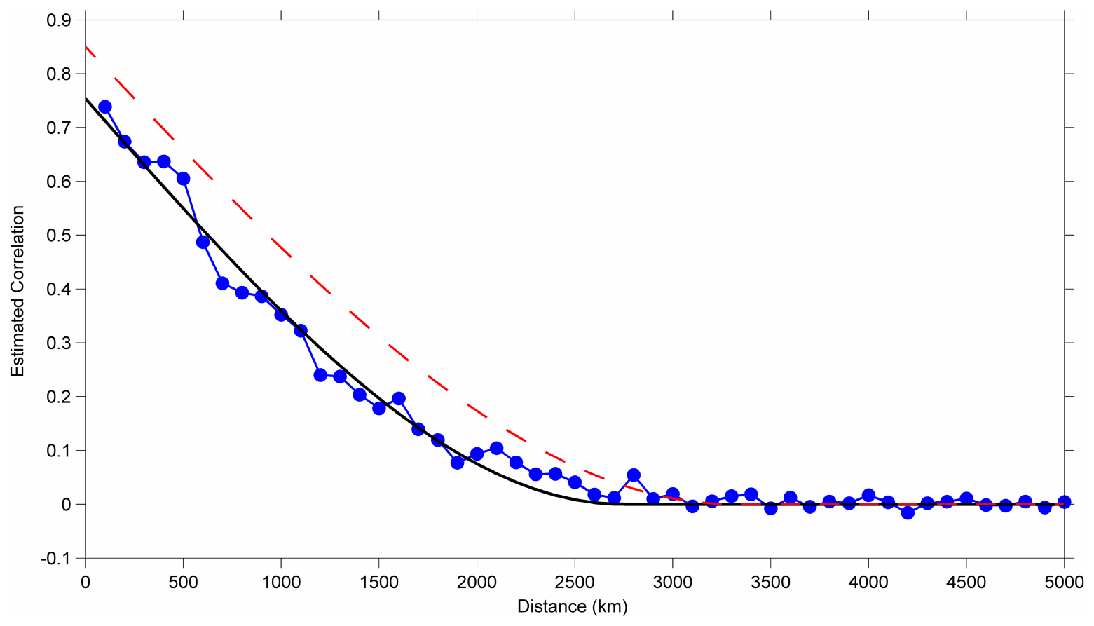
Figure 1Empirically estimated correlation versus distance for monthly average sea surface temperatures. Correlation was estimated by comparing root-mean-square differences for all possible pairs of HadSST grid cells and all months and binning the population by distance. The black curve reflects a best fit for the spherical correlation function model. The red dashed curve shows the corresponding correlation model derived for land-based measurements (Rohde et al., 2013a).
Analogous to Rohde et al. (2013a), the core of the interpolation approach is to generate a kriging-based field using an assumed distance-based correlation function. As with Rohde et al. (2013a), a correlation-based approach is used rather than the more common covariance-based approach to simplify the computational considerations and should be adequate as long as the variance changes relatively slowly with changes in position. A review of both the HadSST data and climate model outputs suggested that the temperature-to-distance correlation function could be modeled effectively via the same spherical correlation function approach used for land surface temperatures:
The empirically estimated distance parameter dmax was found to have a value of 2680 km based on the spatial variance of the HadSST monthly averages. This is similar to, though somewhat smaller than, the 3310 km scale adopted in the land surface temperature study (Rohde et al., 2013a). By contrast, the local correlation parameter R0=0.47 was estimated to be much lower in the oceans (compared to 0.86 on land). This is due to two factors. Firstly, ocean observations are individual measurements whereas land observations reflect monthly averages. Secondly, the typical monthly fluctuations in the oceanic environment are much smaller than on land, causing a reduced signal-to-noise ratio. The estimation of R0 was based on a comparison of the variance in HadSST grid cells with a single measurement to those with > 100 observations. The latter condition provides a proxy for cells where the random portion of measurement and sampling uncertainty could plausibly be neglected.
Figure 1 shows an empirically estimated average correlation versus distance between HadSST grid cells. This shows the empirical length scale, though a larger intercept is used (∼ 0.75), reflecting the fact that the average HadSST grid cell incorporates many observations. The lower value for R0 represents the typical relationship between a single measurement and the monthly average.
This treatment, using a single scale length for the whole ocean, simplifies the analysis; however, it does ignore some of the real variations across the oceans. For example, in regions with boundary currents, upwelling–downwelling, or complex ocean-to-land geographies, the scale length of monthly average temperature variations may be smaller than suggested here. In practice, the 5 ∘ × 5∘ gridding of HadSST already precludes a detailed analysis of most small features. The interpolation presented here primarily serves to improve the representation by smoothing over noise and filling gaps, but it will not necessarily capture the smallest features.
The distance correlation function gives rise to a kriging formulation.
Here t is the current month, T(x,t) is the interpolated temperature at a general location x, SST(xj,t) is the HadSST anomaly value in the grid cell centered at location xj, σm(xj,t) is the measurement uncertainty associated with location xj, and sm is the average measurement uncertainty of a single measurement. Neff(xj,t) is then an effective number of independent measurements associated with the grid cell. Though HadSST provides the true number of observations per cell, N(xj,t), we found that Neff(xj,t), which incorporates the measurement uncertainty, appeared to give superior results than simply relying on the reported number of observations. The incorporation of Neff(xj,t) into the determination of the kriging coefficients K has the effect of giving greater weight to grid cells with less uncertainty. For integer values of Neff(xj,t), the formulation of D(xj,t) is mathematically equivalent to having xj appear Neff(xj,t) independent times in the correlation matrix. Note also that any empty HadSST grid cells at time t are omitted from the matrix formulation for K.
θt is a free parameter at each time t and effectively represents the global ocean-average temperature anomaly. Its value is found iteratively by insisting that the spatial average of .
It is instructive to note that this kriging formulation has the property that in the limit that , but will ordinarily produce a temperature estimate based on a weighted average of multiple HasSST grid points in the case that Neff(xj,t) is small or moderate. The latter property can be useful in suppressing noise at grid locations with high uncertainty and/or very few measurements.
It is also important to recognize that though the correlation function R(d) has a very long tail, this does not mean that average necessarily extends over a large area. In general, the kriging coefficients constructed in this way will heavily favor the nearest several data points. As long as nearby data are available, little weight will be given to distant grid cells. However, the long tail of the correlation function means that the kriging will attempt to fill large holes using distant data if no nearby data are available.
An absolute value field was also created by applying a similar interpolation to the HadSST climatology.
C(x,m) is the interpolated climatology for month m, SSTCLIM(xj,m) is the reported climatology, and is a set of kriging parameters, which are the same as except that R0 and D(xj,t) are both replaced with 1, effectively treating the SSTCLIM(xj,m) as if it has no uncertainty. P(xm) is a background prediction function dependent only on the month and the latitude of x. It is described as a piecewise cubic spline with 11 knots as free parameters equally spaced in the cosine of latitude. These free parameters are chosen to minimize the spatial average of . By construction, for all xj values, and this construction merely provides a way of interpolating between grid cell centers.
In addition to the above description, a physical cutoff was applied to the absolute temperature at a fixed minimum temperature of −1.8 ∘C, which is the freezing temperature of seawater. If the interpolation would suggest a value lower than this, T(x,t) was adjusted accordingly to maintain the minimum value of −1.8 ∘C. Such adjustments are rare.
Finally, one last interpolation is performed using an assumption of temporal persistence. Unlike land temperature anomalies, where the temporal correlation is often only a couple weeks, ocean temperature anomalies typically have a temporal correlation measured in months. This can be exploited to estimate ocean temperatures based on adjacent months when no other information is available.
Analogous to Rohde et al. (2013a), a diagnostic criterion can be constructed . Because of the nature of the kriging coefficients, in the presence of dense data and if there are no HadSST data in the neighborhood of x.
The final estimate of the SST, including a temporal persistence adjustment for regions of low V(x,t), is then
Here, t−1 and t+1 refer to the temperature field 1 month earlier and 1 month later, respectively. This adjustment allows for a modest reduction in uncertainty at early times when data are temporally sparse.
As described, this analysis is agnostic about the resolution used to sample the final temperature field. In practice, we generally use the same 15 984-element equal-area grid as Rohde et al. (2013a) to calculate Tfinal(x,t), though with non-ocean elements masked out.
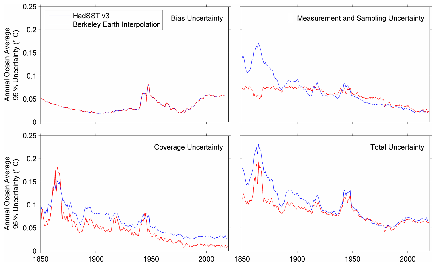
Figure 2Component uncertainties for the ocean average of HadSST v3 and the corresponding transformed forms of those components after the application of the interpolation scheme described in the text. All uncertainties are expressed as appropriate for 95 % confidence intervals on annual ocean averages.
2.2 Ocean uncertainty
The ocean-average uncertainty in our ocean reconstruction is estimated following essentially the same model as adopted by HadSST3. HadSST3 estimates the total reconstruction uncertainty as the combination of measurement uncertainty, coverage uncertainty, and bias uncertainty (Kennedy et al., 2011a, b). Bias uncertainty, σbias, which reflects biases created due to variations over time in the ways that SST has been measured, is brought forward essentially unchanged by our analysis process (Fig. 2). Due to its slowly varying nature, this uncertainty remains the most important limitation of the detection of long-term averages.
The coverage uncertainty, σcoverage, is the uncertainty in the large-scale average arising due to incomplete sampling of the spatial field. As with HadSST3, our estimate of the coverage uncertainty is constructed by sampling a known field, applying our interpolation procedure, and seeing how well we reproduce the underlying average of the known field. Following HadSST3, we used the SST fields provided by HadISST v2 as our target. The HadISST fields are spatially complete, observation-based historical reconstructions of SST and sea ice concentration (Titchner and Rayner, 2014). To estimate the coverage uncertainty associated with a specified HadSST sampling field, we mask every month of the HadISST dataset using that sampling field, interpolate the remaining data, and measure the error in the interpolated average relative to the true ocean average of the whole HadISST field. The deviations in the ocean average are then collected across all HadISST months, and the uncertainty for that coverage mask is reported as the root-mean-square average of the deviations. Using this technique, which is directly analogous to the HadSST3 coverage assessment technique, we estimate that the application of our interpolation approach typically reduces the coverage uncertainty by 20 %–40 % (Fig. 2).
Lastly, we consider the impact of our interpolation on the measurement and sampling uncertainty. Measurement uncertainty essentially captures the errors in individual observations, while sampling uncertainty reflects the fact that water temperatures can vary on timescales shorter than a month and spatial scales smaller than a grid box. Though interpolation does not change the underlying uncertainty associated with individual measurements, by adjusting the weight of individual observations in the overall average, we affect the way that individual measurement errors propagate into the global average. In particular, in the presence of sparse data, limited measurements may be extrapolated over a large area. In some circumstances, this can cause the effective uncertainty in the global average due to these uncertainties to increase. In essence, the interpolation may trade improvements in coverage uncertainty against a greater impact for measurement uncertainty. This largely limits our ability to reduce the overall uncertainty by interpolation.
The impact of measurement uncertainty on a large-scale average depends on the error correlation. If the measurement uncertainties were uncorrelated, then the error would generally be expected to decline with the square root of the number of measurements. In actuality, the measurement uncertainties are frequently correlated. In most cases, single ships report many measurements per month. Each of those measurements can have both random errors and a potential for systematic bias. For a single ship, we cannot expect this bias component of a measurement error to be reduced by increasing the number of observations. In their analysis HadSST3 models the entire error correlation matrix to understand the effect of measurement errors on the global average uncertainty.
For HadSST3, the error correlation matrices were not published. As a result, it is not possible to exactly determine the effect of our interpolation procedure on the measurement uncertainty. However, we can make a reasonable estimate. Since HadSST3 releases both the per-grid-cell measurement uncertainties and the global average measurement uncertainty, we can compare the expected measurement uncertainty treating all grid cells as independent to what is actually observed by HadSST3 using the whole error correlation matrix (Kennedy et al., 2011b).
where A(xj) is the fraction of the Earth's oceans represented by grid cell xj and σuncorrelated is the measurement uncertainty resulting from assuming that the measurement errors in individual grid cells are uncorrelated with other grid cells.
We find that the measurement uncertainty reported by HadSST3 in the ocean average is typically ∼ 2.1 times larger than σuncorrelated, with some variation over time.
We use this estimate as a benchmark to approximate the effect of error correlation on our analysis of measurement uncertainty.
Here the double integral denotes the integral over the surface of the ocean. Thus is effectively the weight of the xj grid point in the global average.
The total uncertainty in the ocean average is then found by assuming the components are independent.
Over nearly all time periods, we find that interpolation does reduce the uncertainty associated with missing coverage. In the early period, the interpolation results in an appreciable reduction in total uncertainty. However, the total uncertainty in the global average is little changed in the recent period. This is because the bias and measurement uncertainties play a dominant role in the recent period, and the impact of these uncertainties on the global average is little changed as a result of the interpolation. However, even if the ocean-average uncertainty is not changed during the recent period, the interpolation may still aid in the interpretation of local- to regional-scale features.
2.3 Land and ocean combination
The combined field is constructed by merging the Berkeley Earth land surface temperature with the interpolated SST field described above. Two versions are considered that differ only in their treatment of sea ice, using either the land air temperature (LAT) or the SST field to estimate the temperature anomaly at sea ice locations. From 1850 to near present, the sea ice locations are estimated using the ice concentration fields in HadISST v2 (Titchner and Rayner, 2014).
To combine LAT and SST data, both data sets are expressed on the same grid. To simplify the combination at cells that are part land and part ocean, we have taken to adding in the spatial climatology and doing the combination in absolute temperatures.
In the case where sea ice areas are represented by SST, the combination is straightforward:
where L(x) is the fraction of the grid cell at location x that is land, and TLAT and TSST are respectively the LAT as estimated by Rohde et al. (2013a) and the interpolated SST as described above.
In the case where sea ice regions are treated as land,
where I(x,t) is the ice fraction at location x at time t as reported by HadISST v2 (Titchner and Rayner, 2014). For this purpose, HadISST is also regridded onto the same grid as LAT and SST. As HadISST is frequently delayed by a few months compared to other climate data, it is necessary to supplement this data set when producing near-real-time estimates. For this purpose, the Sea Ice Index of the National Snow and Ice Data Center (Fetterer et al., 2017) is used for months that are not yet available in HadISST. The modern ice distribution in both HadISST and the Sea Ice Index are based on satellite observations; however, we found that the Sea Ice Index tended to have systematically more partial melting than HadISST. To maintain consistency, a distribution transform was applied to the sea ice fractions provided in the Sea Ice Index based on comparing the 2014–2018 ice fields in each dataset.
It is useful to note that regardless of whether one is using SST or LAT to estimate temperatures in association with sea ice, most such estimates involve a considerable extrapolation. In the case of LAT, for example, conditions over sea ice in the Arctic will usually be extrapolated from Greenland, Canada, Scandinavia, and Russia. Similarly, in the Antarctic, coastal stations will be extrapolated outward over the ice. By contrast, when using SST, one extrapolates from rare SST measurements that may be far removed from the sea ice edge. Or, in the case that analysis of the sea ice regions is excluded entirely, averaging methods are effectively substituting the ocean or global average temperature anomaly.
It is our belief that the anomaly field generated by extrapolating air temperatures over sea ice locations is a more sensible approach to characterizing climate change at the poles. The air temperature changes over the sea ice can be quite large even while the water temperatures underneath are not changing at all. In particular, over the last decades Arctic air has shown a very large warming trend during the winter.
Regardless of the approach used, the spatial climatology can then be calculated and removed (differing from the original only in cells with a mix of land and water/sea ice). Then the long-term trend in the climate can be computed using the spatial average of the anomaly fields.
Uncertainties for the combined record are calculated by assuming the uncertainties in LAT and SST time series are independent and can be combined in proportion to the relative area of land and ocean. In the case that LAT is used over sea ice, the uncertainties for both LAT and SST have to be slightly recalculated by assuming that the time-varying mask is applied the relevant spatial averages in the uncertainty estimations described in Rohde et al. (2013a) and in the SST section above. Doing this adjustment causes a slight increase in LAT uncertainty (due to the extrapolation over sea ice) and a similar small decrease in SST uncertainty.
The Berkeley Earth Land/Ocean temperature product will be updated monthly on the berkeleyearth.org website and is freely available for use to all interested researchers. A convenience copy of the dataset available at the time this paper was created has been registered with Zenodo and is available at https://doi.org/10.5281/zenodo.3634713 (Rohde and Hausfather, 2020).
The global mean anomalies obtained from the Berkeley Earth Land/Ocean Temperature Record are quite similar to other published records, as shown in Fig. 3. With the exception of some short periods prior to 1880 and before and after World War 2, all four other temperature records examined lie within the uncertainty envelope of the Berkeley Earth record. Differences around World War 2 relate primarily to differences in adjustments to ERSST v5 and HadSST3 sea surface temperature records during that period (Huang et al., 2017; Kennedy et al., 2019; Cowtan et al., 2017).
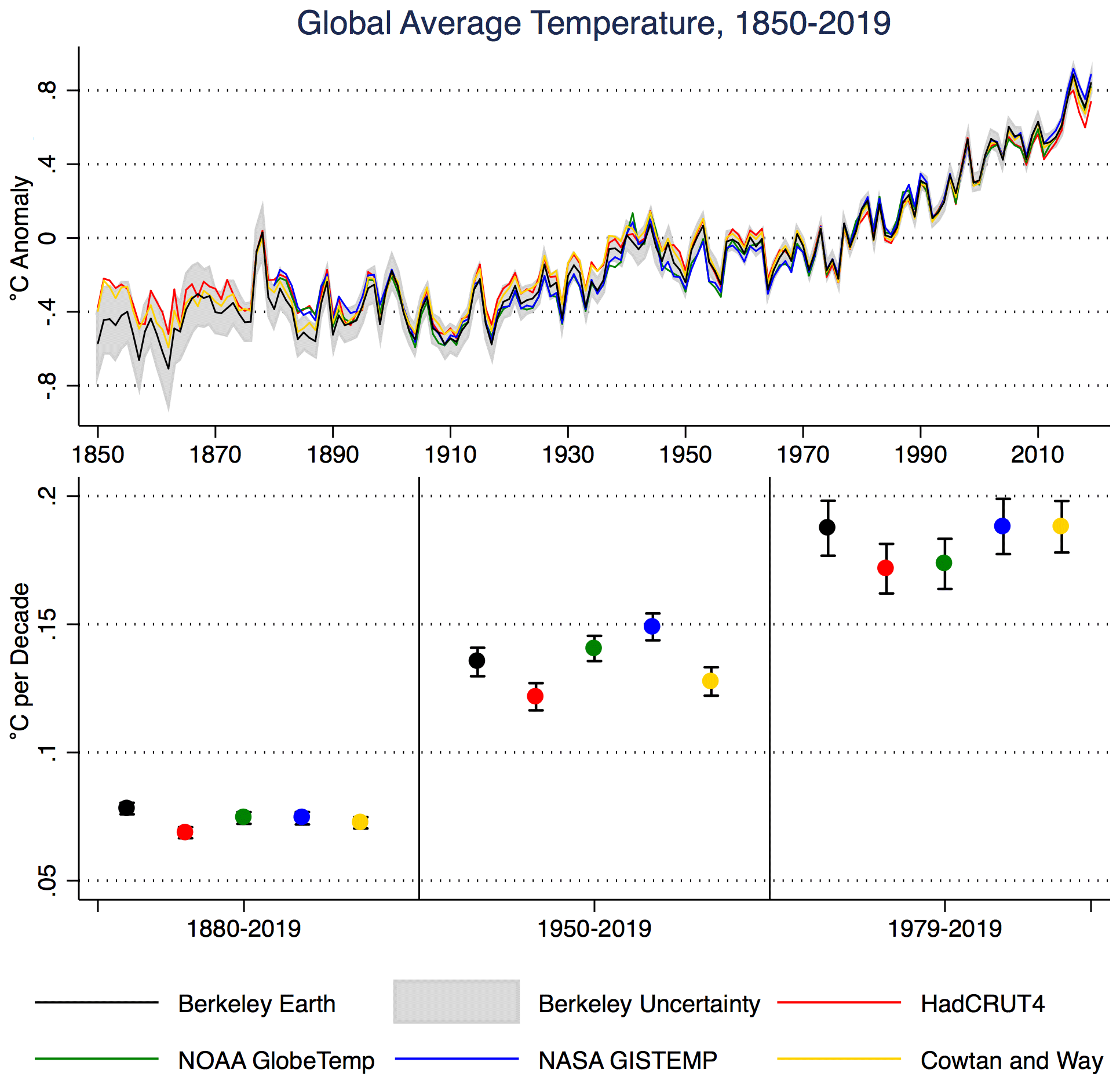
Figure 3Comparison of published global surface temperature records. The top panel shows annual anomalies (relative to a 1961–1990 baseline period), with the Berkeley Earth uncertainty as the shaded area. The bottom panel shows trends and two-sigma trend uncertainties (calculated using an autoregressive–moving average, ARMA(1,1), approach to account for autocorrelation) for various starting dates through the end of 2015 based on monthly anomalies.
Berkeley Earth has the highest trend of any temperature record examined for the period from 1880 to 2015, largely due to lower surface temperature estimates prior to 1900. These differences are driven both by increased spatial coverage from the inclusion of additional land records and by the spatial interpolation of both land and ocean records (which are more limited in both the NOAA and Hadley records). Similarly, Berkeley Earth has among the highest warming rates in the recent period (1979–2015) due primarily to greater Arctic coverage (where warming was unusually rapid during that period). The other records that provide robust Arctic interpolation, CW2014 and NASA GISTEMP, also show higher trends during this period.
From 1955 to present (after the availability of data in Antarctica), Berkeley Earth provides globally complete coverage via spatial interpolation, similar to NASA's GISTEMP and CW2014. This contrasts with HadCRUT4 which excludes any grid cells lacking station coverage or SST measurements, or NOAA GlobalTemp where interpolation is more limited. As shown in Fig. 4, the patterns of spatial anomalies between the different groups tend to be quite similar, apart from differences due to spatial coverage or gridded field resolution.
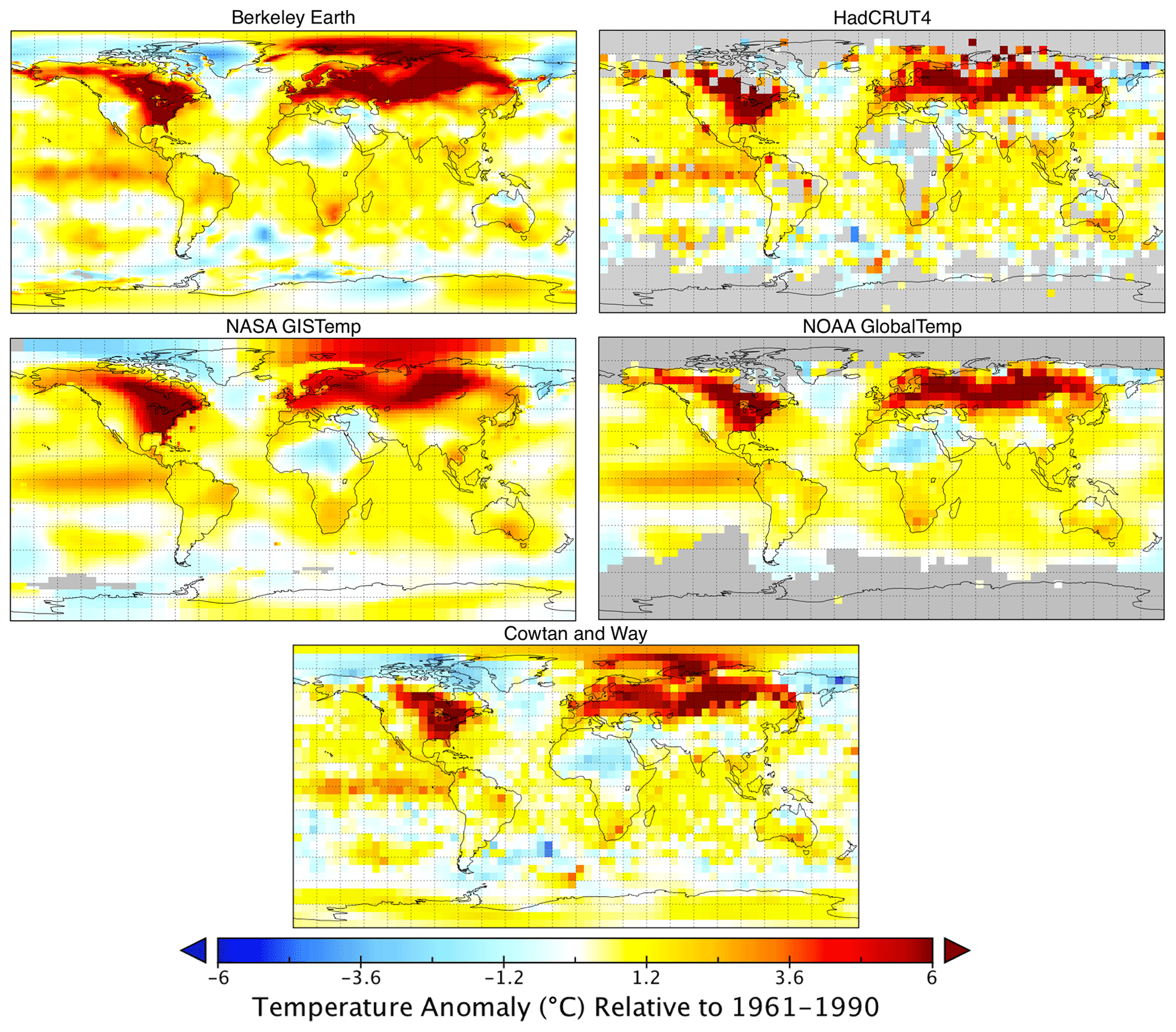
Figure 4Global gridded temperature anomalies for December 2015 relative to a 1961–1990 baseline for each global temperature dataset. Grid resolution is based on the highest-resolution dataset provided by each group: lat–long for Berkeley Earth, for HadCRUT4, for NASA GISTEMP, over land and over oceans for NOAA GlobalTemp, and for Cowtan and Way (CW2014).
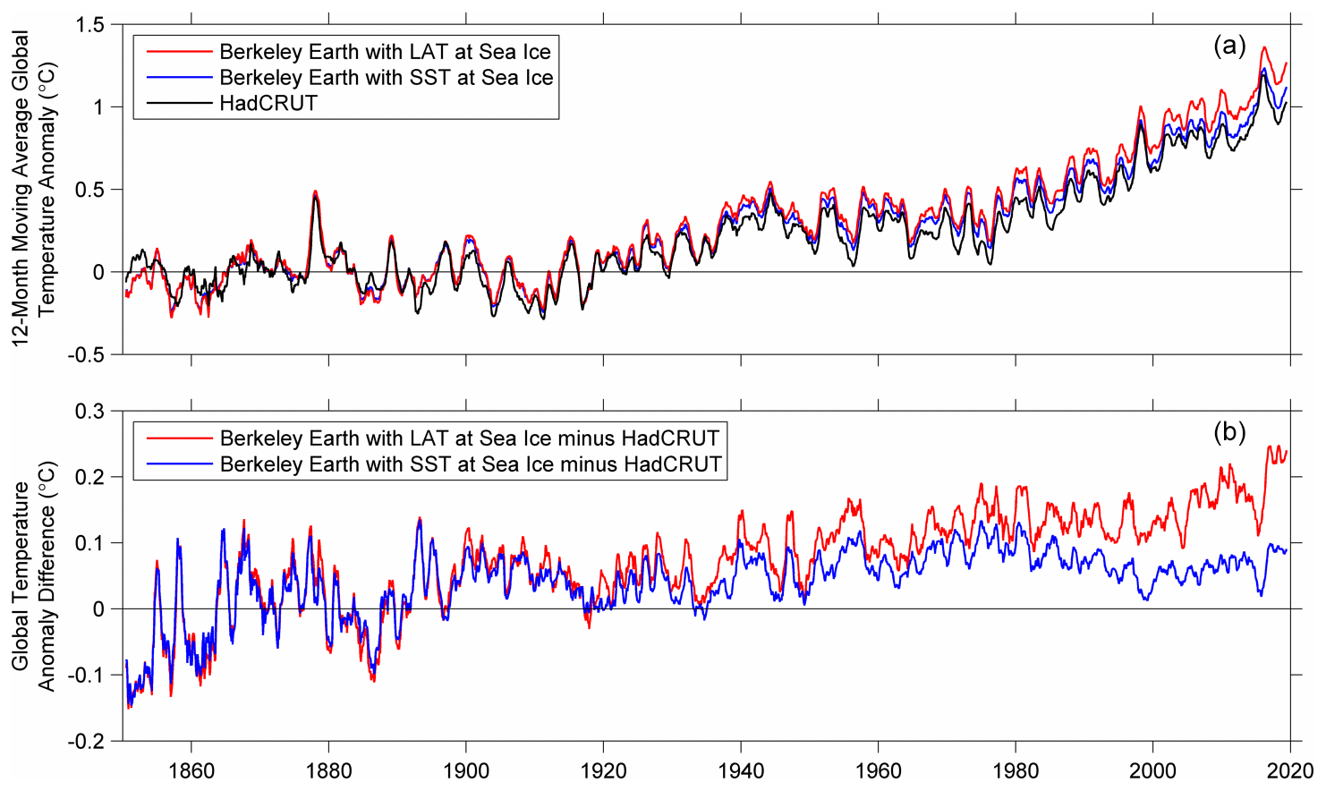
Figure 5(a) Two variants of the Berkeley Earth global surface temperature product estimating temperatures under sea ice based on SSTs (red) or proximate air temperature measurements (blue), as well as the HadCRUT temperature series for comparison. (b) The same two versions of the Berkeley Earth data set with the HadCRUT time series subtracted.
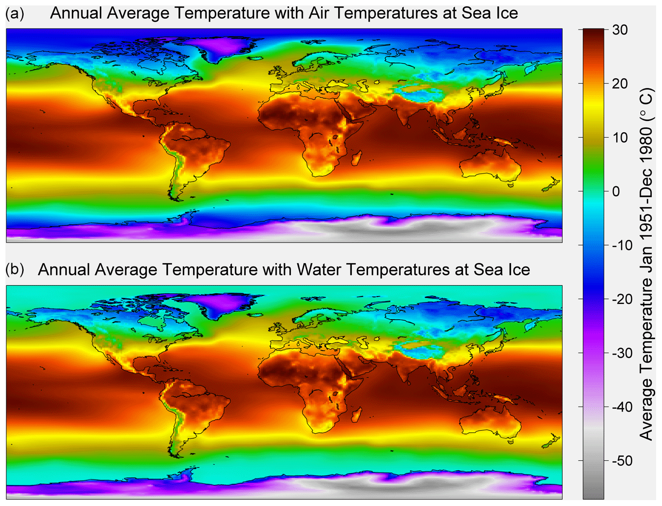
Figure 6Berkeley Earth average absolute climatology for the period from 1951 to 1980 with the air temperature at sea ice (a) and ocean temperature under sea ice (b) variants shown.
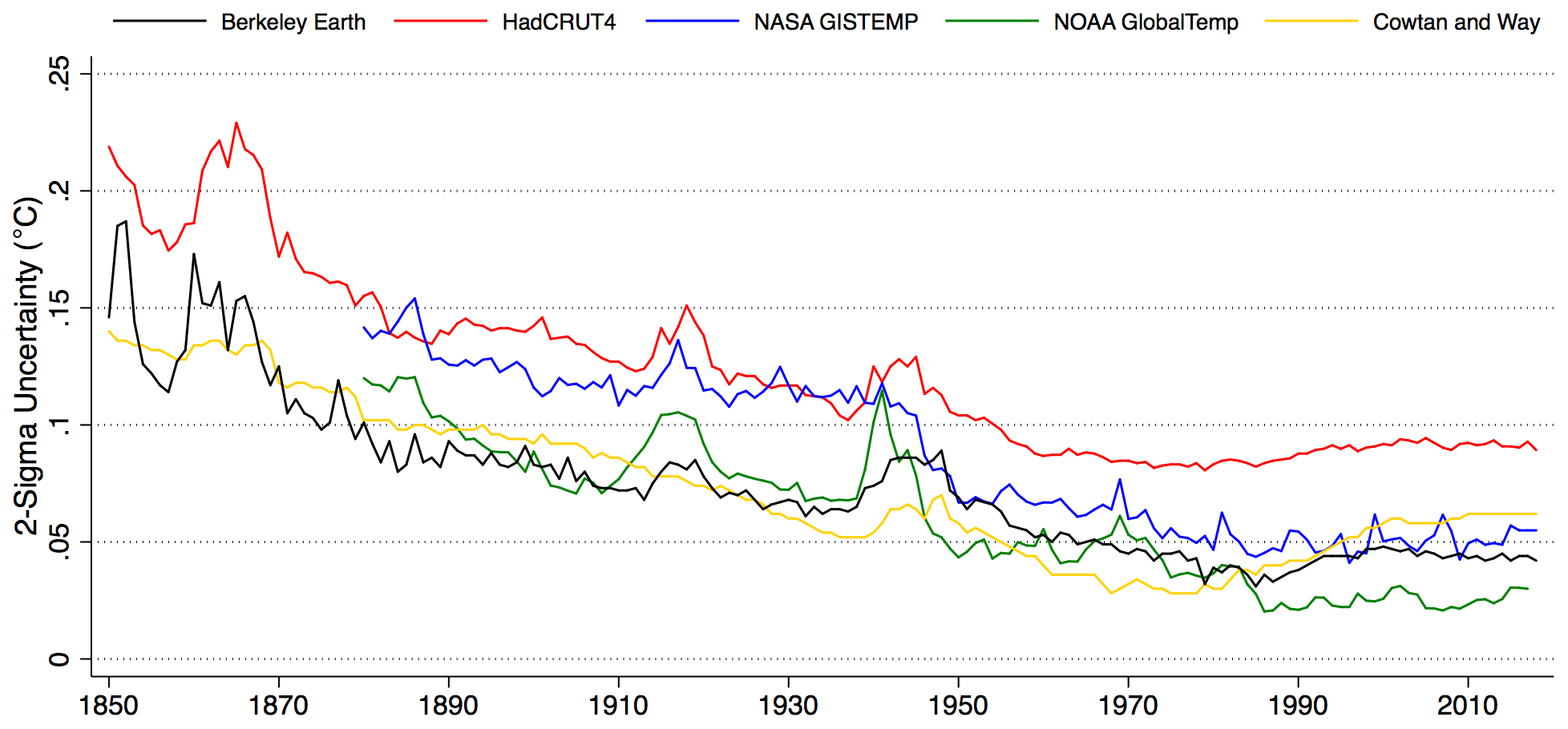
Figure 7Comparison of published annual uncertainty estimates (two sigma) for Berkeley Earth, HadCRUT4 (Morice et al., 2012), GISTEMP (Lenssen et al., 2019), GlobalTempv5 (Vose et al., 2012), and Cowtan and Way (2014).
When constructing a global surface temperature record, sea ice produces a challenging edge case. The water temperature under sea ice is tightly constrained by the freezing point of water and can only change with changes in sea ice cover. Air temperatures over sea ice are less well constrained and can vary significantly over time. Whether areas with sea ice coverage are estimated using sea surface temperatures or surface air temperatures will have a notable effect on the record. While most groups (GISTEMP, CW2014) that interpolate temperatures over areas with sea ice cover use air temperatures, Berkeley Earth has provided both variants to allow researchers to select the series that best supports their needs. We consider the variant using air temperature above sea ice to be a better description of global climate change, but the ocean temperature variants may be useful for comparison and for certain specialists. Both variants of the Berkeley Earth record are shown in Fig. 5 as well as the HadCRUT temperature series for comparison. When SSTs under sea ice are used, the apparent warming trend in recent years is lower than when air temperatures are used. Comparing these versions helps to reveal the contribution of sea ice areas to the overall global warming rate.
Figure 5 also aids in understanding the difference between Berkeley Earth and HadCRUT. The interpolated SST field adopted here has a nearly identical trend to the HadSST field, differing by less than 0.01 ∘C per century. Part of the difference between Berkeley Earth's global temperature series and HadCRUT is due to differences in the amount of warming estimated to have occurred over land. This is the primary source of difference when comparing the Berkeley Earth series with SST at sea ice to the HadCRUT series (blue line in Fig. 5). While this difference is not insignificant, the larger overall difference is due to the incorporation of air temperature warming in sea ice regions, especially in the Arctic (red line in Fig. 5). Inclusion of the rapid warming above Arctic sea ice suggests the global average has increased an additional ∼ 0.1 ∘C during the last 100 years compared to estimates that do not include the changes in this region.
In addition to monthly temperature anomalies, Berkeley Earth produces monthly absolute temperature fields. A climatology field is estimated via kriging observations, using elevation as a factor in the kriging process over land. Both absolute temperature variants with air temperature over sea ice and water temperature under sea ice are available, as shown in Fig. 6. Absolute temperatures are created by adding the climatology field to monthly anomalies.
Figure 7 provides a comparison between published uncertainties (two sigma) for each of the major global land–ocean temperature series. The Berkeley Earth, GISTEMP, and CW2014 records have the lowest uncertainty of the groups providing annual values, in part due to their spatial interpolation reducing the uncertainty associated with coverage.
The Berkeley Earth Land/Ocean surface temperature record presented here has already been used by a number of publications (e.g., Jones, 2015; Thorne et al., 2016; Sutton et al., 2015). It joins a number of existing land–ocean surface temperature products that help provide a diverse examination of the Earth's changing climate since 1850 and can be used for diverse applications including climate model validation, estimating transient climate response, examining changes in extreme events, and other research areas.
RR designed and implemented the dataset construction. ZH provided feedback, graphics, and analysis. RR and ZH jointly prepared the manuscript.
The authors declare that they have no conflict of interest.
This paper was edited by David Carlson and reviewed by two anonymous referees.
Cowtan, K. and Way, R. G.: Coverage bias in the HadCRUT4 temperature series and its impact on recent temperature trends, Q. J. Roy. Meteor. Soc., 140, 1935–1944, 2014.
Cowtan, K., Hausfather, Z., Hawkins, E., Jacobs, P., Mann, M. E., Miller, S. K., Steinman, B. A., Stolpe, M. B., and Way, R. G.: Robust comparison of climate models with observations using blended land air and ocean sea surface temperatures, Geophys. Res. Lett., 42, 6526–6534, https://doi.org/10.1002/2015GL064888, 2015.
Cowtan, K., Rohde, R., and Hausfather, Z.: Evaluating biases in sea surface temperature records using coastal weather stations, Q. J. Roy. Meteor. Soc., 144, 670–681, https://doi.org/10.1002/qj.3235, 2017.
Fetterer, F., Knowles, K., Meier, W. N., Savoie, M., and Windnagel, A. K.: Sea Ice Index, Version 3. Boulder, Colorado USA, NSIDC: National Snow and Ice Data Center, https://doi.org/10.7265/N5K072F8, 2017.
Freeman, E., Woodruff, S. D., Worley, S. J., Lubker, S. J., Kent, E. C., Angel, W. E., Berry, D. I., Brohan, P., Eastman, R., Gates, L., Gloeden, W., Ji, Z., Lawrimore, J., Rayner, N. A., Rosenhagen, G., and Smith, S. R.: ICOADS Release 3.0: A major update to the historical marine climate record, Int. J. Climatol. 37, 2211–2237, https://doi.org/10.1002/joc.4775, 2017.
Hansen, J., Ruedy, R., Sato, M., and Lo, K.: Global Surface Temperature Change, Rev. Geophys., 48, RG4004, https://doi.org/10.1029/2010RG000345, 2010.
Huang, B., Thorne, P. W., Banzon, V. F., Boyer, T., Chepurin, G., Lawrimore, J. H., Menne, M. J., Smith, T. M., Vose, R. S., and Zhang, H.-M.: Extended Reconstructed Sea Surface Temperature, Version 5 (ERSSTv5): Upgrades, Validations, and Intercomparisons, J. Clim., 30, 8179–8205, https://doi.org/10.1175/JCLI-D-16-0836.1, 2017.
Huang, B., Menne, M. J., Boyer, T., Freeman, E., Gleason, B. E., Lawrimore, J. H., Liu, C., Rennie, J. J., Schreck, C. J., Sun, F., Vose, R., Williams, C. N., Yin, X., and Zhang, H.-M.: Uncertainty Estimates for Sea Surface Temperature and Land Surface Air Temperature in NOAAGlobalTemp Version 5, J. Clim., 33, 1351–1379, https://doi.org/10.1175/JCLI-D-19-0395.1, 2020.
Ishihara, K.: Calculation of Global Surface Temperature Anomalies with COBE-SST, (Japanese) Weather Service Bulletin 73, 2006.
Ishii, M., Shouji, A., Sugimoto, S., and Matsumoto, T.: Objective analyses of sea-surface temperature and marine meteorological variables for the 20th century using ICOADS and the Kobe Collection, Int. J. Climatol., 25, 865–879, 2005.
Jones, P.: The Reliability of Global and Hemispheric Surface Temperature Records, Adv. Atmos. Sci., 33, 1–14, 2015.
Jones, G. S.: “Apples and Oranges”: on comparing simulated historic near surface temperatures changes with observations, Q. J. Roy. Meteor. Soc., https://doi.org/10.1002/qj.3871, 2020.
Kennedy, J. J., Rayner, N. A., Smith, R. O., Parker, D. E., and Saunby, M: Reassessing biases and other uncertainties in sea surface temperature observations measured in situ since 1850: 2. Biases and homogenization, J. Geophys. Res.-Atmos., 116, D14104, https://doi.org/10.1029/2010JD015220, 2011a.
Kennedy J. J., Rayner, N. A., Smith, R. O., Saunby, M., and Parker, D. E.: Reassessing biases and other uncertainties in sea-surface temperature observations since 1850 part 1: measurement and sampling errors, J. Geophys. Res.-Atmos., 116, D14103, https://doi.org/10.1029/2010JD015218, 2011b.
Kennedy, J. J., Rayner, N. A., Atkinson, C. P., and Killick, R. E.: An Ensemble Data Set of Sea Surface Temperature Change From 1850: The Met Office Hadley Centre HadSST.4.0.0.0 Data Set, J. Geophys. Res.-Atmos., 124, 7719–7763, https://doi.org/10.1029/2018JD029867, 2019.
Kent, E. C., Rayner, N. A., Berry, D. I., Saunby, M., Moat, B. I., Kennedy, J. J., and Parker, D. E.: Global analysis of night marine air temperature and its uncertainty since 1880: the HadNMAT2 Dataset, J. Geophys. Res.-Atmos., 118, 1281–1298, https://doi.org/10.1002/jgrd.50152, 2013.
Lawrimore, J. H., Menne, M. J., Gleason, B. E., Williams, C. N., Wuertz, D. B., Vose, R. S., and Rennie, J.: An overview of the Global Historical Climatology Network monthly mean temperature data set, version 3, J. Geophys. Res., 116, D19121, https://doi.org/10.1029/2011JD016187, 2011.
Lenssen, N. J. L., Schmidt, G. A., Hansen, J. E., Menne, M. J., Persin, A., Ruedy, R., and Zyss, D.: Improvements in the GISTEMP Uncertainty Model, J. Geophysi. Res.-Atmos., 124, 6307–6326, https://doi.org/10.1029/2018JD029522, 2019.
Menne, M. J. and Williams, C. N.: Homogenization of temperature series via pairwise comparisons, J. Clim., 22, 1700–1717, 2009.
Menne, M. J., Williams, C. N., Gleason, B. E., Rennie, J. J., and Lawrimore, J. H.: The Global Historical Climatology Network Monthly Temperature Dataset, Version 4, J. Clim., 31, 9835–9854, https://doi.org/10.1175/JCLI-D-18-0094.1, 2018.
Morice, C. P., Kennedy, J. J., Rayner, N. A., and Jones, P. D.: Quantifying uncertainties in global and regional temperature change using an ensemble of observational estimates: The HadCRUT4 data set, J. Geophys. Res.-Atmos., 117, D08101, https://doi.org/10.1029/2011JD017187, 2012.
Morice, C. P., Kennedy, J. J., Rayner, N. A., Winn, J. P., Hogan, E., Killick, R. E., Dunn, R. J. H., Osborn, T. J., Jones, P. D., and Simpson, I. R.: An updated assessment of near-surface temperature change from 1850: the HadCRUT5 dataset, J. Geophys. Res., submitted, 2020.
Richardson, M., Cowtan, K., Hawkins, E., and Stolpe, M. B.: Reconciled climate response estimates from climate models and the energy budget of Earth, Nat. Clim. Change, 6, 931–935, https://doi.org/10.1038/nclimate3066, 2016.
Rohde, R. and Hausfather, Z.: Berkeley Earth Combined Land and Ocean Temperature Field, Jan 1850–Nov 2019, Zenodo, https://doi.org/10.5281/zenodo.3634713, 2020.
Rohde, R., Muller, R. A., Jacobsen, R., Muller, E., Perlmuller, S., Rosenfeld, A., Wurtele, J., Groom, D., and Wickham, C.: A New Estimate of the Average Earth Surface Land Temperature Spanning 1753 to 2011, Geoinfor. Geostat. Overv., 1, 1–7, https://doi.org/10.4172/2327-4581.1000101 2013a.
Rohde, R., Muller, R. A., Jacobsen, R., Perlmuller, S., Rosenfeld, A., Wurtele, J., Curry, J., Wickham, C., and Mosher, S.: Berkeley Earth Temperature Averaging Process, Geoinfor. Geostat. Overv., 1, 2, https://doi.org/10.4172/2327-4581.1000103, 2013b.
Smith, T. M., Reynolds, R. W., Peterson, T. C., and Lawrimore, J.: Improvements to NOAA's Historical Merged Land–Ocean Surface Temperature Analysis (1880–2006), J. Climate, 21, 2283–2296, 2008.
Sutton, R., Suckling, E., and Hawkins, E.: What does global mean temperature tell us about local climate?, Philos. T. R. Soc. A, 373, 2054, 2015.
Thorne, P. W., Donat, M. G., Dunn, R. J. H., Williams, C. N., Alexander, L. V., Caesar, J., Durre, I., Harris, I., Hausfather, Z., Jones, P. D., Menne, M. J., Rohde, R., Vose, R. S., Davy, R., Klein-Tank, A. M. G., Lawrimore, J. H., Peterson, T. C., and Rennie, J. J.: Reassessing changes in diurnal temperature range: Intercomparison and evaluation of existing global data set estimates, J. Geophys. Res.-Atmos. 121, 5138–5158, 2016.
Titchner, H. A. and Rayner, N. A.: The Met Office Hadley Centre sea ice and sea surface temperature data set, version 2: 1. Sea ice concentrations, J. Geophys. Res.-Atmos., 119, 2864–2889, https://doi.org/10.1002/2013JD020316, 2014.
Vose, R. S., Arndt, D., Banzon, V. F., Easterling, D. R., Gleason, B., Huang, B., Kearns, E., Lawrimore, J. H., Menne, M. J., Peterson, T. C., Reynolds, R. W., Smith, T. M., Williams, C. N., and Wuertz, D. B.: NOAA's Merged Land–Ocean Surface Temperature Analysis, B. Am. Meteorol. Soc., 93, 1677–1685, 2012.