the Creative Commons Attribution 4.0 License.
the Creative Commons Attribution 4.0 License.
 | 17 Dec 2020
Subglacial topography and ice flux along the English Coast of Palmer Land, Antarctic Peninsula
Emily A. Hill
G. Hilmar Gudmundsson
John Woodward
Recent satellite data have revealed widespread grounding line retreat, glacier thinning, and associated mass loss along the Bellingshausen Sea sector, leading to increased concern for the stability of this region of Antarctica. While satellites have greatly improved our understanding of surface conditions, a lack of radio-echo sounding (RES) data in this region has restricted our analysis of subglacial topography, ice thickness, and ice flux. In this paper we analyse 3000 km of 150 MHz airborne RES data collected using the PASIN2 radar system (flown at 3–5 km line spacing) to investigate the subglacial controls on ice flow near the grounding lines of Ers, Envisat, Cryosat, Grace, Sentinel, Lidke, and Landsat ice streams as well as Hall and Nikitin glaciers. We find that each outlet is topographically controlled, and when ice thickness is combined with surface velocity data from MEaSUREs (Mouginot et al., 2019a), these outlets are found to discharge over 39.25 ± 0.79 Gt a−1 of ice to floating ice shelves and the Southern Ocean. Our RES measurements reveal that outlet flows are grounded more than 300 m below sea level and that there is limited topographic support for inland grounding line re-stabilization in a future retreating scenario, with several ice stream beds dipping inland at ∼ 5∘ km−1. These data reinforce the importance of accurate bed topography to model and understand the controls on inland ice flow and grounding line position as well as overall mass balance and sea level change estimates. RES data described in this paper are available through the UK Polar Data Centre: https://doi.org/10.5285/E07D62BF-D58C-4187-A019-59BE998939CC (Corr and Robinson, 2020).
- Article
(12888 KB) - Full-text XML
- BibTeX
- EndNote


Remote sensing satellites have increased our awareness and understanding of ice flows in Antarctica since their inception. In western Palmer Land, on the Antarctic Peninsula, Earth observation satellites have recorded widespread grounding line retreat (Christie et al., 2016; Konrad et al., 2018) and surface lowering (attributed to glacier thinning) in the last 2 decades (Wouters et al., 2015; Hogg et al., 2017; Smith et al., 2020), as well as surface velocity increases and significant mass loss (e.g. McMillan et al., 2014; Wouters et al., 2015; Martín-Español et al., 2016; Hogg et al., 2017), where ice flows contribute ∼ 0.16 mm a−1 to global mean sea level (Wouters et al., 2015). Regional mass losses of −56 ± 8 Gt a−1 between 2010 and 2014 (Wouters et al., 2015) exceed the magnitude of interannual variability predicted by surface mass balance models (van Wessem et al., 2014, 2016), suggesting that the English Coast of western Palmer Land is undergoing significant change. While satellites have greatly improved our understanding of surface conditions and changes across Antarctica in recent years, a lack of ice thickness and subglacial topographic measurements in western Palmer Land has restricted our analysis of the controls on ice flow, ice flux, and grounding line stability along the English Coast (Minchew et al., 2018). As subglacial topography exerts a strong control over ice flow, it is critical to collect and analyse radio-echo sounding (RES) data close to the grounding line in understudied regions of Antarctica.
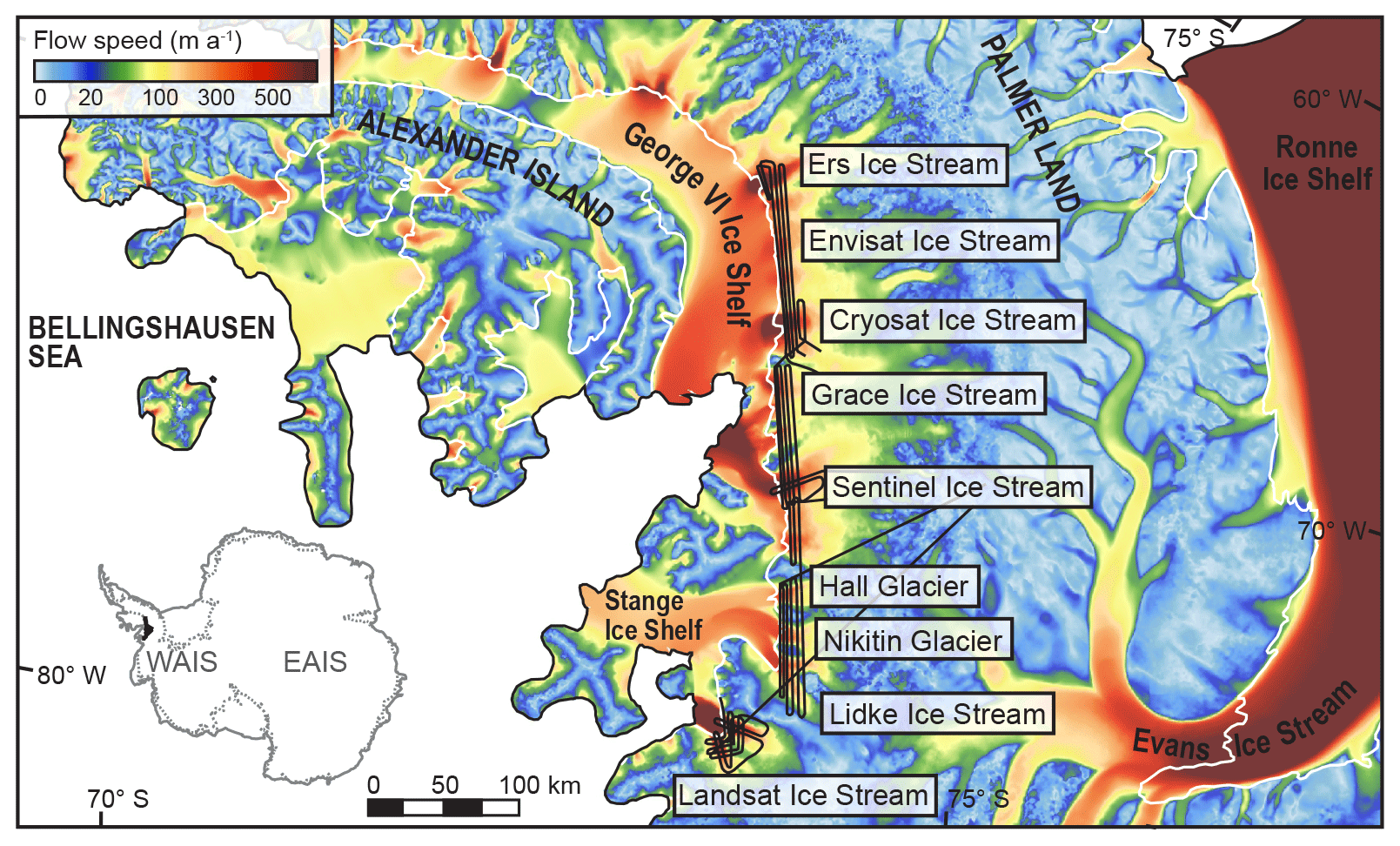
Figure 1Airborne radio-echo sounding surveys (RES) (black lines), collected during the austral summer of 2016/2017, transcend the Bellingshausen Sea sector of Palmer Land in the Antarctic Peninsula. RES surveys transect several glaciers and ice streams along the English Coast at or close to the Antarctic Surface Accumulation and Ice Discharge (ASAID) grounding line (white line) (Bindschadler et al., 2011), after which the ice floats. Background imagery shows surface flow speeds from MEaSUREs (Mouginot et al., 2019a). The inset map shows the location of RES surveys used in this paper (black), superimposed on a map of Antarctica.
In this paper we present a new, freely available RES dataset along the English Coast of western Palmer Land, where several outlet glaciers were named after Earth observation satellites in 2019, in deference to the critical role that satellites have played in measuring and monitoring the Antarctic Ice Sheet (Fig. 1). We combine this new geophysical dataset with satellite measurements of ice flow speeds from MEaSUREs (Mouginot et al., 2019a) to provide an improved picture of the subglacial controls on ice flows draining the English Coast, and we directly assess the improvements to our understanding of bed topography and ice flux in the region as a result of such high-resolution RES datasets.
The English Coast of western Palmer Land contains numerous outlet glaciers which flow at speeds of ∼ 0.5 to 2.5 m d−1 (Mouginot et al., 2019a), from accumulation areas in central Palmer Land towards ice shelves in the Bellingshausen Sea sector of Antarctica (Fig. 1). A map of surface ice flow speeds in Fig. 1 shows how the recently named Ers, Envisat, Cryosat, and Grace ice streams drain into the fast-flowing George VI Ice Shelf, where floating ice connects Palmer Land to Alexander Island. Further south, Sentinel Ice Stream passes the local grounding line to form a floating tongue, connected in part to the neighbouring George VI Ice Shelf. Moving south of George VI Ice Shelf, Hall Glacier, Nikitin Glacier, and Lidke Ice Stream each flow into Stange Ice Shelf. Whilst these outlet flows have separate accumulation zones that border the large Evans Ice Stream catchment (which drains into the Weddell Sea, on the other side of the Antarctic Peninsula) (Fig. 1), their distinct flow units converge along the English Coast, at the local grounding zone. At the southern extremity of the English Coast, Landsat Ice Stream flows close to the catchment-defined boundary between the Antarctic Peninsula and West Antarctica. Slow-flowing, almost stagnant ice separates the two tributary flows of Landsat Ice Stream for much of its length (Mouginot et al., 2019a).
Our understanding of the English Coast of western Palmer Land is driven by data accessibility. Fast ice flow and heavily crevassed surfaces have largely restricted in situ data collection in this region. The first Antarctic-wide ice thickness and subglacial topography datasets Bedmap (Lythe et al., 2001) and Bedmap2 (Fretwell et al., 2013) relied on sparse RES measurements for interpolation in this region of Antarctica. As a result, there are large uncertainties in bed topography and ice thickness along the English Coast, which limit our understanding of regional ice dynamics (Minchew et al., 2018). Inaccurate ice thickness and bed topography also hinder our ability to assess the sensitivity of this region to future change using numerical ice flow models. Previous work has therefore made use of more readily available satellite data, such as optical images, altimeter data, and synthetic-aperture radar (SAR) measurements to assess regional change. Numerous studies have used these detailed datasets to report on and model recent changes in surface elevation and ice flow along the Bellingshausen Coast (e.g. Pritchard et al., 2012; Christie et al., 2016; Hogg et al., 2017; Minchew et al., 2018), as well as Antarctica as a whole (e.g. Helm et al., 2014; McMillan et al., 2014; Konrad et al., 2018; Smith et al., 2020). Collectively, this work has highlighted a number of potential vulnerabilities in western Palmer Land. Recent mass loss of George VI Ice Shelf and Stange Ice Shelf (totalling an estimated 11 Gt a−1) (Rignot et al., 2019) raised concern that English Coast outlet glaciers could be susceptible to the marine ice sheet instability mechanism (Wouters et al., 2015) – where grounding-lines have a tendency to accelerate down a retrograde slope in the absence of compensating forces (like buttressing ice shelves) (Schoof, 2007; Gudmundsson et al., 2012). These concerns are compounded by recent changes in the grounded ice flows along the English Coast. Wouters et al. (2015) reported an average surface lowering of ∼ 0.5 m a−1 along the coastline between 2010–2014, whilst Hogg et al. (2017) calculated a 13 % increase in outlet glacier ice flow between 1993 and 2015. Importantly, if surface thinning and ice flow acceleration across western Palmer Land continue in the future, dynamical imbalance could lead to further draw down of the interior ice sheet (like it has done in other areas of Antarctica; e.g. Shepherd et al., 2002; Rignot 2008; Konrad et al., 2018), leading to increased ice discharge into the ocean (Gudmundsson, 2013; Wouters et al., 2015; Fürst et al., 2016; Kowal et al., 2016; Minchew et al., 2018), with resultant sea level rise. New, high-resolution measurements of ice thickness and subglacial topography close to the grounding line will improve our understanding of ice dynamics along the English Coast, and enable more accurate modelling of current conditions, and forward-looking estimations.
Datasets outlined in Sect. 3.1–3.3 are freely available to download. Download links are provided in Sect. 7.
3.1 Airborne radio-echo-sounding acquisition, processing, and visualization
In the austral summer of 2016/2017, the British Antarctic Survey Polarimetric-radar Airborne Science Instrument (PASIN2) ice sounding radar system was used to acquire ∼ 3000 line km of radio-echo sounding (RES) data along the English Coast of western Palmer Land, at ∼ 3–5 km line spacing (Corr and Robinson, 2020). PASIN2 operates at a frequency of 150 MHz, using a pulse-coded waveform at an effective acquisition rate of 312.5 Hz and a bandwidth of 13 MHz. Technical details of the RES system are available in Corr et al. (2007). Differential GPS was used to record aircraft position (with an accuracy better than ±1 m) and RES data were collected at an average flying velocity of 55 m s−1. Along-track processing of the data results in an output data rate of 5 Hz, which produces an average spacing between radar traces of 11 m. Section 7 details the information we extract from the online data repository for use in this paper.
For the processing of the data, a coherent moving-average filter, commonly referred to as an unfocused SAR, was used on the range compressed data. The onset of the bed reflector was first automatically picked using first-break picker of the ProMAX (version 5000.10.0.0; Landmark Software and Services) seismic processing software with all picks then checked afterwards and corrected by hand if necessary. The delay time of the bed reflector picks were covered to range using a standard electromagnetic wave propagation speed in ice of 0.168 m ns−1 and a correction of 10 m to account for the near-surface high-velocity firn layer (Dowdeswell and Evans 2004; Vaughan et al., 2006). Ice thickness was calculated by subtracting surface elevation measurements (derived from radar/laser altimeters for aircraft terrain clearance) from bed reflector depth picks. Internal crossover analysis (measurements of ice thickness at the same position) yield a standard deviation of 13 m at line intersections, with no systematic line-to line biases. Independent crossover analysis, with NASA's airborne Operation IceBridge (OIB) radar data (Paden et al., 2010) (collected from November 2010–November 2016), yields a higher standard deviation of 48 m (when high-elevation OIB flights are removed from analysis). As this standard deviation is skewed by a relatively small number of high crossover misfits over steep subglacial topography (where the outlet ice flows are located), we use the internal crossover analysis value of 13 m for our RES errors.
RES transects were visualized in 2D in Reflexw radar processing software (version 7.2.2; Sandmeier Scientific Software) where an energy decay gain was applied to compensate for geometric spreading losses in the radargram (Daniels et al., 2004). OpendTect seismic interpretation software (version 6.4.0; dGB Earth Sciences) was employed to plot radargrams in real space using DGPS co-ordinates, to enable three-dimensional analysis of RES data.
3.2 Mapping subglacial topography and ice thickness
Airborne RES data presented in this paper have been incorporated in the new BedMachine dataset; a self-consistent dataset of the Antarctic Ice Sheet based on conservation of mass, which has a resolution of 500 m (Morlighem, 2019; Morlighem et al., 2019). As a result, data presented in this paper have already been combined with numerous other RES survey data (including OIB data) to produce continent-wide ice thickness and subglacial topography maps (Fig. 2b). Whilst Morlighem et al. (2019) report potential vertical errors of ∼ 100 m in central Palmer Land, these values decrease towards the coast, where RES measurements are more frequent (Morlighem, 2019).
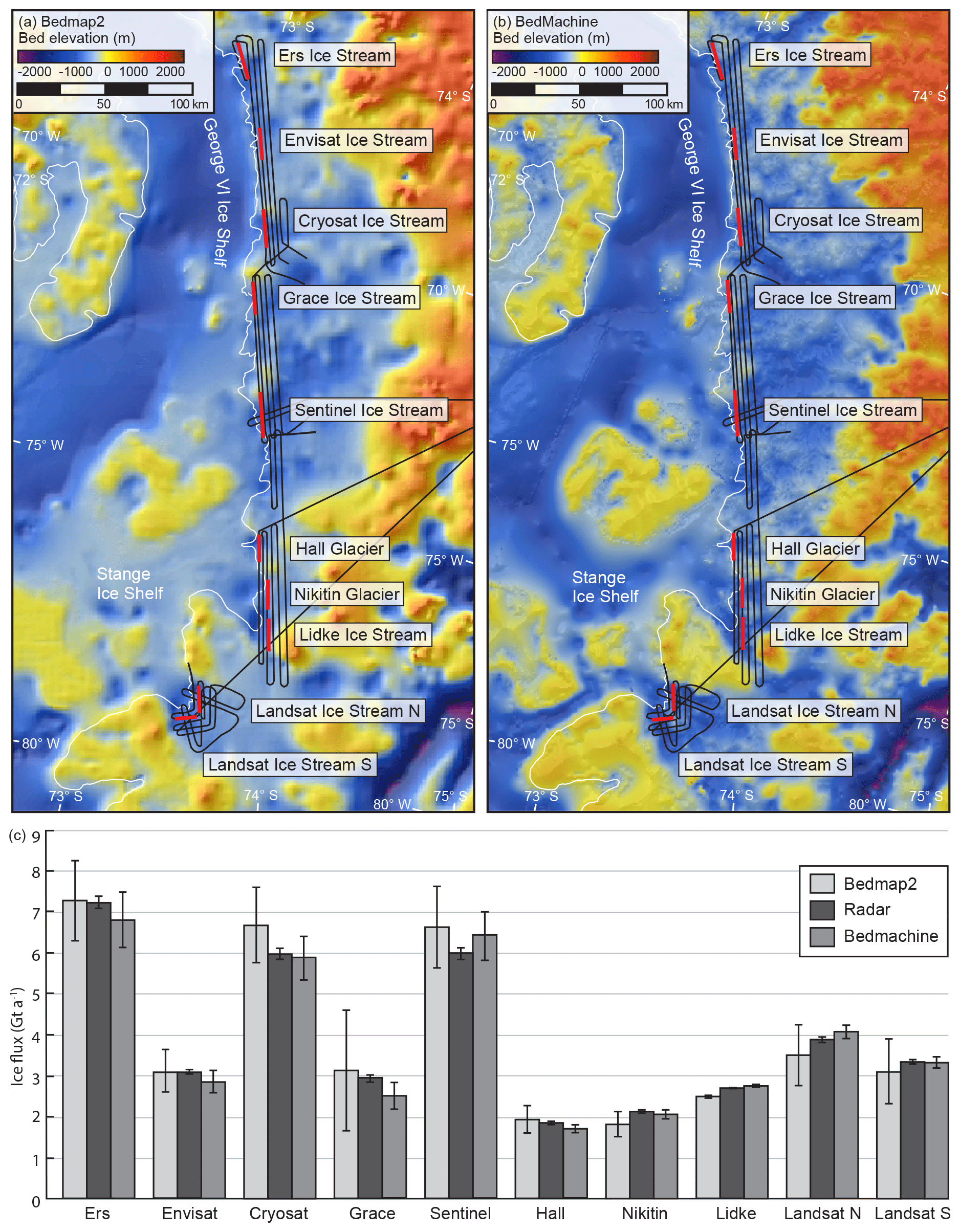
Figure 2Major outlet glacier and ice stream flux gates (red) along the English Coast of Palmer Land. Subglacial topography maps from Bedmap2 (Fretwell et al., 2013) and BedMachine (Morlighem, 2019) are presented in panels (a) and (b). Black lines denote airborne RES transects detailed in this paper, whilst the white line shows the location of the ASAID grounding line (Bindschadler et al., 2011). Both maps show that subglacial topography frequently rests well below sea level along the English Coast. Panel (c) compares ice flux measurements (in metric gigatons), derived from Bedmap2 ice thickness data (Fretwell et al., 2013) (light-grey bars), our direct radar measurements (dark-grey bars), and ice thickness data from BedMachine (Morlighem, 2019) (mid-grey bars). These calculations utilize the same flux gates, noted in panels (a) and (b).
3.3 Surface flow speeds
Surface flow speeds are extracted from MEaSUREs phase-based Antarctica ice velocity map which has a resolution of 450 m (Mouginot et al., 2019a) (Fig. 1a). This dataset combines interferometric phases from multiple satellite interferometric synthetic-aperture radar systems, with additional data, including tracking-derived velocity to maximize coverage from 1996 to 2018 (Mouginot et al., 2019b). Across western Palmer Land the average flow speed error is estimated to be less than 4 m a−1.
3.4 Calculating ice flux
Using surface flow speeds (Mouginot et al., 2019a) and ice thickness measurements from the 1us radargrams in the online data repository (see Sect. 7), we calculate ice flux across fixed gates delineated for each of the named ice streams and glaciers along the English Coast (Fig. 2). These flux gates are delineated along RES transects immediately upstream of the grounding line and they span the width of each outlet. Ice flux (q) for each ice stream or glacier (j) is calculated following Eq. (1):
where i is an equally spaced bin along the length of the flux gate, w is the bin width (which is fixed to 1 m for all outlets and is sufficiently small that the solution is not sensitive to a bin width smaller than this), and v is the velocity normal to the flux gate. We use an ice density value of ρ=917 kg m−3, which is consistent with densities used in both Bedmap2 and BedMachine datasets (Fretwell et al., 2013; Morlighem, 2019). For simplicity, we are assuming that surface velocities and ice density are constant with depth. To examine the impact of incorporating high-resolution RES data into gridded bed topography datasets, we directly compare ice flux from Bedmap2 (Fretwell et al., 2013) (which has a resolution of 1 km) with the radar picks described in Sect. 3.1, which are included in BedMachine (Morlighem, 2019) (Fig. 2c). For these calculations we use the same flux gates, phase-based ice velocities, and ice density, simply replacing RES ice thickness for Bedmap2 ice thickness. Using available errors in velocity and ice thickness datasets, we calculate errors in our calculated ice flux (σq) for each glacier following Eq. (2):
where and are the contribution of errors in velocity (dv) and ice thickness (dh) to the errors in ice flux respectively. Ice flux and associated error bars for each outlet are shown in Fig. 2c.
Our airborne RES transects map subglacial topography and ice thickness down the English Coast, from Ers Ice Stream to Landsat Ice Stream. Whilst our results and discussion focus on seven major outlets, ice flux from each of the named outlets is presented in Fig. 2. The complete RES dataset (marked in Fig. 1) is freely available to download from the UK Polar Data Centre (see Sect. 7 for more details).
4.1 Ers Ice Stream
Close to the grounding line, Ers Ice Stream reaches a maximum flow speed of just over 940 m a−1 (averaging out at ∼ 2.5 m d−1) (Mouginot et al., 2019a). This ice originates from central Palmer Land (Fig. 1), where ice flows across the west of the Antarctic Peninsula, towards Ers Ice Stream. In the upper catchment, flow speeds of ∼ 400 m a−1 (Mouginot et al., 2019a) are recorded along RES transect Ers 6 (Fig. 3a). A succession of airborne RES transects in Fig. 3c show how this fast-flowing ice is channelized towards the coast, through a subglacial depression ∼ 8–14 km wide. As ice flows through this channel, towards the local grounding line (marked in white in Fig. 3a), ice thickness reduces from a maximum of ∼ 1400 m (along transect Ers 6) to between 580 and 610 m (along transect Ers 1), where the ice flow is grounded ∼ 400 m below sea level. Ice flux calculated along this radar transect suggests that Ers Ice Stream contributes over 7.24 ± 0.15 Gt a−1 to George VI Ice Shelf (Fig. 2c). Although this flux gate represents the main trunk of Ers Ice Stream (Fig. 2a, b), neighbouring ice flow from the lateral margins of the ice stream (where ice flows at ∼ 210–390 m a−1) will, of course, add to this value.
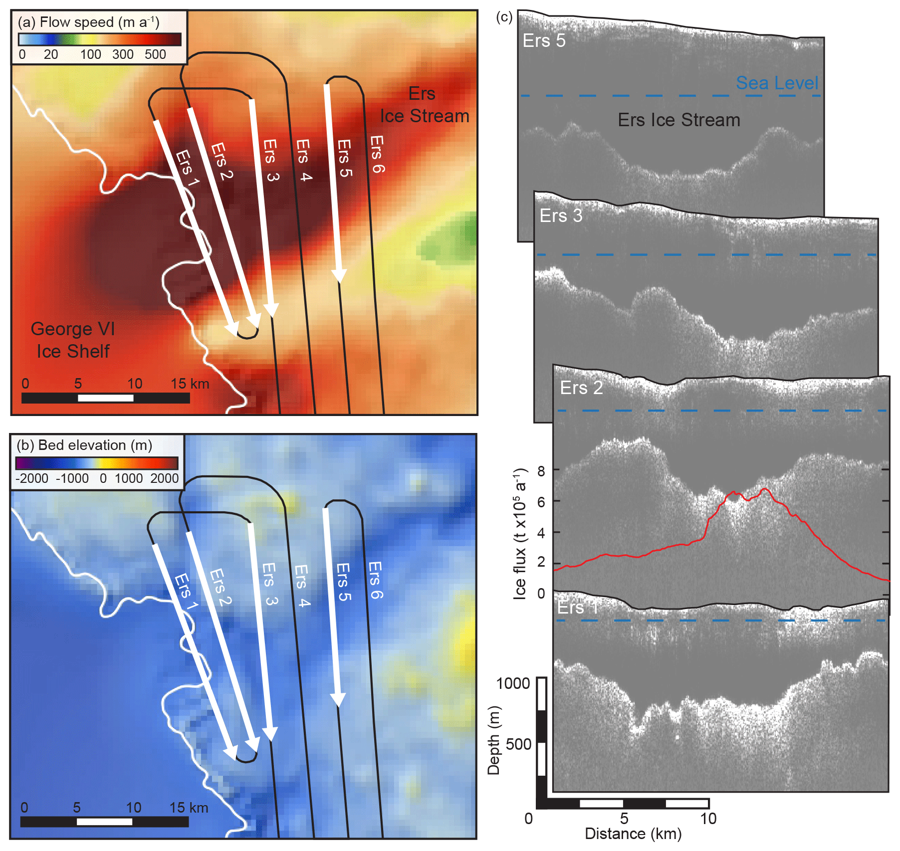
Figure 3Ice-penetrating radar transects (black lines) across Ers Glacier, superimposed on a map of surface flow speeds (Mouginot et al., 2019a) (a) and subglacial topography from BedMachine (Morlighem, 2019) (b). White arrows indicate the location and direction of radargrams presented in panel (c) whilst the white line indicates the ASAID grounding line (Bindschadler et al., 2011). Ice flux across RES transect Ers 2 is displayed as a red line in panel (c). Note that the scale is in tonnes ×105. (c) Radargrams reveal surface topography, ice thickness and the subglacial bed (recorded as diffuse white reflectors). Sea level is marked by a blue dashed line.
4.2 Cryosat Ice Stream
A central flow unit, more than 14 km wide, distinguishes Cryosat Ice Stream from neighbouring regions of slower-flowing ice along the English Coast (Fig. 1). Whilst surrounding ice flows at ∼ 100 m a−1, flow speeds in the ice stream range from 400–500 m a−1 inland (along RES transect Cryosat 3) to 950 m a−1 (∼ 2.6 m d−1) (Mouginot et al., 2019a) along RES transect Cryosat 1 – which was traversed close to the Antarctic Surface Accumulation and Ice Discharge (ASAID) grounding line (Bindschadler et al., 2011) (Fig. 4a). Figure 4a shows how the main flow of Cryosat Ice Stream is joined by a smaller tributary to the south, where ice flow speeds increase from 180 m a−1 along transect Cryosat 4 to over 400 m a−1 (Mouginot et al., 2019a) along transect Cryosat 1 (traversed ∼ 5 km from the ASAID grounding line). In both flow units, the subglacial bed remains well below sea level along the length of each transect. Close to the grounding line, along transect Cryosat 1, the glacial bed is between 450 and 800 m below sea level, where overlying ice is 500–900 m thick. Although subglacial topographic depressions are visible in-land (where subglacial peaks which reach over 500 m from the bed help to define the low-elevation topography), subglacial troughs become more defined towards the coast, where ice is guided through several almost U-shaped troughs (Fig. 4b). This is most obvious in RES transect Cryosat 1, where the main flow of ice is channelled through a ∼ 14 km wide, 300 m deep subglacial trough close to the local grounding line, whilst the smaller (southern) tributary flow is directed through a ∼ 400 m deep trough, which is ∼ 3 km wide at its base (Fig. 4b). The flow units of Cryosat Ice Stream collectively discharge 5.99 ± 0.14 Gt a−1 of ice across the grounding line. The ice flux profile in Fig. 4b shows how much of this flux is discharged through the deep and fast-flowing central sector of the ice stream, rather than the deeper southern tributary.
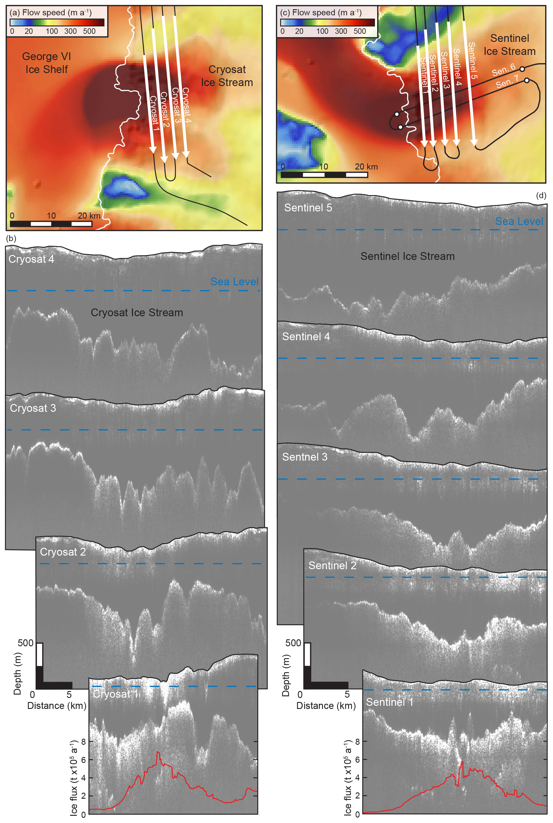
Figure 4Radar investigations of Cryosat and Sentinel ice streams. Surface flow speed maps (Mouginot et al., 2019a) reveal the spatial variability in flow in panels (a) and (c). These panels highlight the location of radargrams collected along the English Coast (black lines) as well as the direction and location of radargrams (white arrows) displayed in panels (b) and (d). White lines indicate the ASAID grounding line (Bindschadler et al., 2011) whilst white circles in panel (c) represent the extent of along-flow radar transects presented in Fig. 7. Red lines in panels (b) and (d) show calculated ice flux along RES transects Cryosat 1 and Sentinel 1. Sea level is marked by a blue dashed line.
4.3 Sentinel Ice Stream
In the MEaSUREs velocity map, Sentinel Ice Stream appears to have the widest outflow of the English Coast, reaching a width of over 20 km. The main trunk of the ice stream curves round from an almost southerly flow direction, to a more westerly direction along its length (Fig. 4c) as ice flow speeds increase from ∼ 350 m a−1 (along RES transect Sentinel 5) to ∼ 800 m a−1 (closer to the grounding zone, along transect Sentinel 1) (Mouginot et al., 2019a). Whilst the subglacial bed remains well below sea level in all transects (at elevations in the region of −500 to −680 m), fluctuations in subglacial topography and ice thickness are recorded along- and down-flow in successive RES transects (Fig. 4d). The largely unconfined ice flow in transect Sentinel 5 becomes more confined down-flow due to the emergence of higher-elevation subglacial topography along the lateral margins of Sentinel Ice Stream. These subsurface conditions are concurrent with ice thickness measurements (where maximum ice thickness decreases down-flow, from ∼ 1200 m in transect Sentinel 5 to ∼ 550 m in Sentinel 1), as well as surface velocity measurements, which reveal increasing flow speeds in the central trunk of Sentinel Ice Stream with distance down-flow. The total flux of Sentinel Ice Stream is 6.01 ± 0.14 Gt a−1. Whilst this flux will be added to by flow from the south (where enhanced flow speeds are recorded, but they are about 3 times slower than the central trunk of Sentinel Ice Stream), there will be much less flux in the north, where ice flows at a few tens of metres per year (Mouginot et al., 2019a) (Fig. 4c), over higher-elevation subglacial topography (∼ 400 m higher than the base of the subglacial trough).
4.4 Hall Glacier
Hall Glacier is the most northern tributary flow of the Stange Ice Shelf (Fig. 1). Surface flow speeds increase from RES transect HNL 6 (close to the onset of streaming flow) – where ice flows just over 100 m a−1, to RES transect HNL 1 (∼ 1.5–9.5 km from the ASAID grounding line and 14 km from HNL 6), where ice flow speeds reach 380 m a−1 (Mouginot et al., 2019a) (Fig. 5a). These enhanced flow speeds clearly differentiate Hall Glacier from the almost stagnant neighbouring ice flow (< 10 m a−1) along its lateral margins in Fig. 5a. This figure shows how the fast-flowing portion of the outlet glacier decreases in width from ∼ 15 km inland to ∼ 8 km along RES transect HNL 2. This reduction in width coincides with a change in subsurface topography and ice thickness (Fig. 5c). Whilst a shallow subglacial depression is apparent upstream, in RES transect HNL 5 (where the subglacial bed is ∼ 500 m below sea level and ice thickness reaches a maximum of 750 m), a much deeper channel is recorded down-flow, where ice up to 930 m thick is channelized through high-elevation subglacial topography. The profile in Fig. 5b (derived from the flux gate marked in Fig. 5a) shows the impact this subglacial topography and ice thickness have on ice flux. Flux is greatest along the central trunk of Hall Glacier where a ∼ 7 km wide subglacial channel supports ice flow speeds of more than 350 m a−1 (Mouginot et al., 2019a). Over the whole flux gate, Hall Glacier contributes ∼ 1.87 ± 0.04 Gt a−1 of ice to the Stange Ice Shelf, which drains into the Bellingshausen Sea sector of the Southern Ocean.
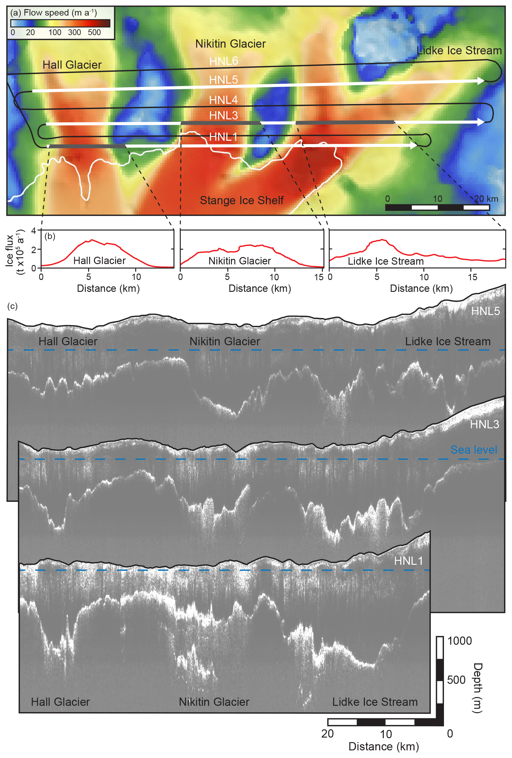
Figure 5Hall Glacier, Nikitin Glacier, and Lidke Ice Stream transfer fast-flowing ice to the local grounding line (white), where ice flow coalesces in the Stange Ice Shelf. (a) Surface flow speeds from Mouginot et al. (2019a), superimposed with English Coast radargram tracks (black). The white arrows indicate the location and direction of radargrams presented in panel (c), and thick grey lines denote ice flux gates, graphed in panel (b). The white line indicates the ASAID grounding line (Bindschadler et al., 2011). Note that the map has been rotated 90∘ from its true orientation (shown in Fig. 1). Radargrams in panel (c) reveal changes in ice thickness and subglacial topography down-flow. Sea level is marked by a blue dashed line.
4.5 Nikitin Glacier
Situated between Hall Glacier and Lidke Ice Stream, Nikitin Glacier maintains flow speeds in the region of 200–450 m a−1 (Mouginot et al., 2019a), as ice flow from central Palmer Land begins to stream towards the Stange Ice Shelf (Fig. 5). For much of its length, Nikitin Glacier flows through a 15 km wide subglacial channel, where ice thicknesses up to 1000 m flow over a glacial bed situated well below sea level (with elevations of −400 to −700 m). This low-elevation subglacial topography combined with thick ice flows and enhanced ice flow speeds enable Nikitin Ice Stream to contribute over 2.13 ± 0.05 Gt a−1 of ice to the Stange Ice Shelf. Whilst it is difficult to precisely define the point at which this ice begins to float in our radargrams, it is worth noting that complex and highly reflective RES returns beneath Nikitin Ice Stream in transect HNL 1 suggest that the ice stream could be afloat here. This finding is coincident with the positioning of the ASAID grounding line (Bindschadler et al., 2011) (marked as a white line in Fig. 5a), which is derived from satellite data.
4.6 Lidke Ice Stream
The MEaSUREs dataset (Mouginot et al., 2019a) presented in Fig. 5a, shows how Lidke Ice Stream is fed by two tributary flows which coalesce close to RES transect HNL 4, where ice begins to flow along a central trunk at flow speeds in the region of 350–420 m a−1 (Fig. 5a). Although Lidke Ice Stream is linked to neighbouring Nikitin Ice Stream in its upper catchment, a clear separation between the two ice streams is recorded down-flow, where the enhanced flow units become separated by a region of almost stagnant ice (< 10 m a−1). RES transects in Fig. 5c show how this slow-moving ice sits on top of relatively high-elevation subglacial topography (with elevations of −380 to −500 m). This raised topography helps to define the northern margin of Lidke Ice Stream, which flows through much lower-elevation subglacial topography, situated ∼ 600–800 m below sea level.
In RES transects HNL 4 and HNL 5 (traversed close to the onset of streaming flow) numerous peaks and troughs dominate the subglacial topography returns, resulting in spatially variable ice thickness and ice flux. However, further down-flow, and closer to the grounding line, subglacial topography is more subdued, with the emergence of a depressed subglacial channel (reaching a maximum depth of 810 m below sea level), where ice up to 1250 m thick achieves surface flow speeds in the region of 400 m a−1 (Mouginot et al., 2019a) at the grounding zone. In a flux gate along HNL3 (marked in Fig. 5a), Lidke Ice Stream is calculated to contribute > 2.71 ± 0.01 Gt a−1 to the Stange Ice Shelf. The flux profile in Fig. 5b shows how this value is distributed across the glacier – with high flux values recorded in areas which have low-elevation subglacial topography, thicker ice, and fast ice flow.
4.7 Landsat Ice Stream
Landsat Ice Stream (situated close to the catchment-defined boundary between the Antarctic Peninsula and West Antarctica) is formed of a northern and southern tributary, with ice flow converging at or close to the ASAID grounding line (Fig. 6). Both tributaries have similar characteristics: they each reach flow speeds in excess of 500 m a−1 in the centre of the ice flow (along RES transect Landsat 3) before flow begins to accelerate downstream (to over 700 m a−1 near transect Landsat 1) (Mouginot et al., 2019a). Between the two tributaries, flow speeds are much lower, ranging from 40 m a−1 (25 km inland of the grounding line) to ∼ 100 m a−1 (along RES transect Landsat 1, traversed close to the local grounding line) (Mouginot et al., 2019a). A sequence of airborne RES transects in Fig. 6c show that these flow speeds reflect subglacial topography. Both tributaries flow through deep subglacial basins (situated ∼ 700 m below sea level), where ice flows up to 900 m thick are increasingly channelized towards the coast by higher subglacial topography along the ice stream's lateral margins. Along RES transect Landsat 2, ice flux gates across the north and south tributary flows combine to produce a total ice flux of 7.23 ± 0.13 Gt a−1. Between these two flow units ice flux is substantially lower, because of lower surface flow speeds, elevated subglacial topography, and reduced ice thickness.
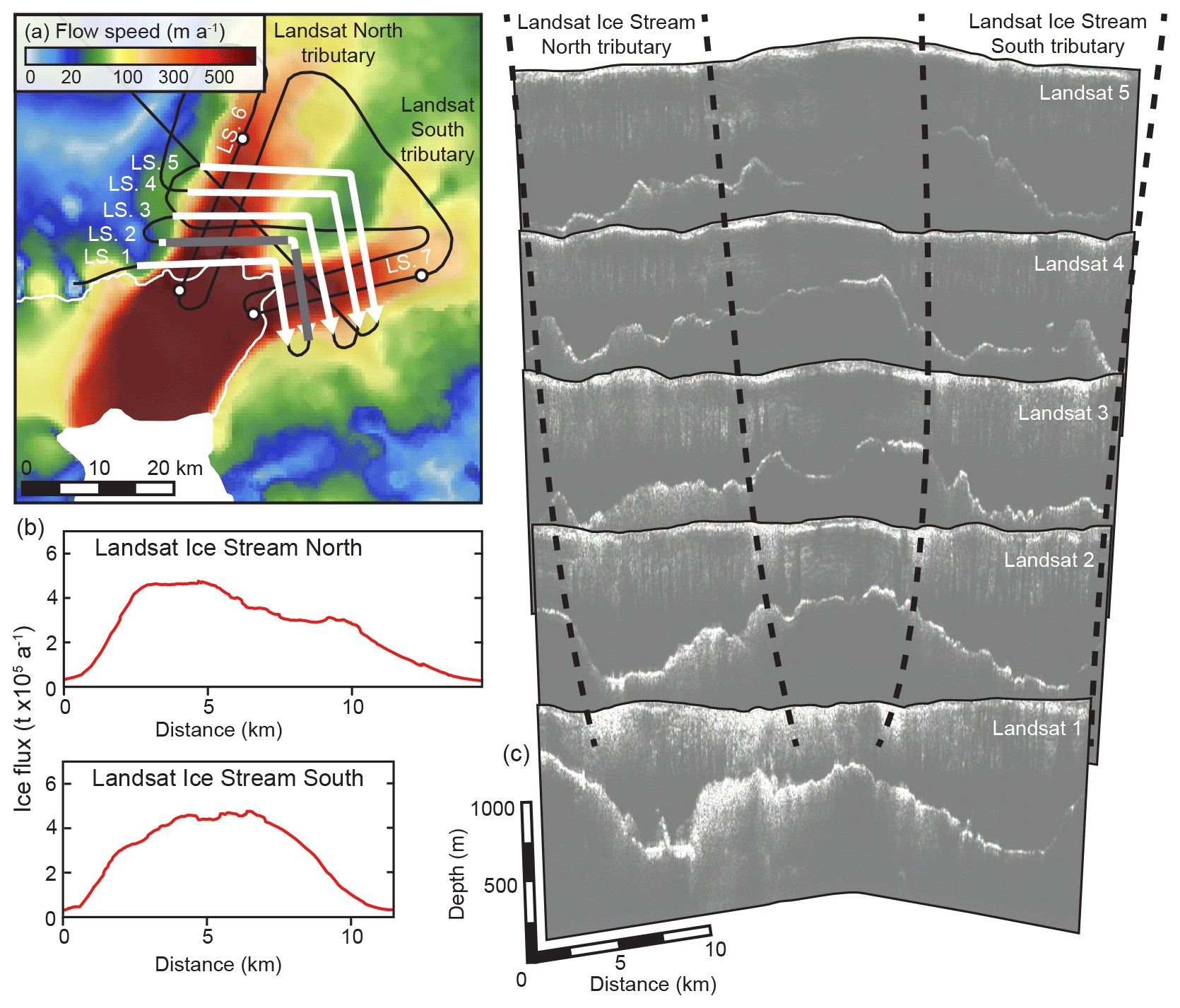
Figure 6Landsat Ice Stream is fed by northern and southern tributaries, which coalesce at the grounding zone. These discrete flow units are clearly visible in panel (a) which shows a map of surface flow speeds from Mouginot et al. (2019a). Black lines show the density of RES transects in this location, whilst white arrows show the location and orientation of transects displayed in panel (c). In panel (a) the white line represents the ASAID grounding line (Bindschadler et al., 2011) whilst thick grey lines show the location of flux gates, presented in panel (b). White circles in panel (a) represent the extent of along-flow radar transects presented in Fig. 7 (where sea level is marked along each tributary). Radargrams in panel (c) show how the two ice stream tributaries (approximately marked by a black dashed line) are separated by relatively high-elevation subglacial topography.
English Coast ice streams and glaciers contribute over 39.25 ± 0.79 Gt a−1 of ice to floating ice shelves in the Bellingshausen Sea. This ice flows from the centre of Palmer Land, towards the coast, where discrete ice flows develop in line with and as a result of depressed subglacial topography – in a region of Antarctica where the glacial bed is situated well below sea level. In the following paragraphs, we briefly discuss the main features of each major ice stream (documented in the results) from north to south. The significance of the radar dataset is presented in Sect. 6.
5.1 Ers Ice Stream
Ers Ice Stream, at the northern extremity of our study site, produces the largest ice flux of all English Coast ice streams (Fig. 2c). This is the result of elevated surface flow speeds (Mouginot et al., 2019a), substantial ice thicknesses, and pronounced subglacial topography, which, for the most part, channelizes ice through a wide subglacial depression (Fig. 3c). Enhanced ice flow is also recorded on either side of the subglacial channel, where surface flow speeds greater than 100 m a−1 (Mouginot et al., 2019a) contribute over 1 × 10⁻⁴ Gt of ice to George VI Ice Shelf per year. This enhanced ice flow makes it difficult to precisely map the lateral margins of the ice stream and fully assess the individual contribution of Ers Ice Stream to English Coast ice flux. However, it is clear that this area of the English Coast contributes substantial and continued ice flux to George VI Ice Shelf, as a result of high surface flow speeds, thick ice, and deep subglacial topography.
5.2 Cryosat Ice Stream
Although ice flux from Cryosat Ice Stream is more than 50 % lower than that of neighbouring Ers Ice Stream, it boasts the greatest surface flow speeds of the English Coast: flowing at a maximum of 950 m a−1 (Mouginot et al., 2019a) (averaging out at ∼ 2.6 m d−1). These enhanced ice flow speeds are recorded along the width of the ice stream, where thick ice flows through and over multiple deep incisions in the basal topography (Fig. 4b). Figure 4a shows how these ice flow speeds are maintained across the grounding zone, as ice flows into George VI Ice Shelf. As the ice shelf buttresses the inland ice flow of Cryosat Ice Stream, further thinning of the ice shelf could reduce resistive stress (buttressing) at the grounding line, subsequently increasing ice discharge in this region (Tsai et al., 2015; Minchew et al., 2018).
5.3 Sentinel Ice Stream
Pronounced topographic depressions in most of the cross-flow radar lines that transect Sentinel Ice Stream (Fig. 4d) suggest a degree of topographic confinement for Sentinel Ice Stream, which is grounded more than 500 m below sea level. Whilst this confinement helps to channelize 6.00 Gt a−1 of ice towards the local grounding line currently, along-flow radargrams in Fig. 7a show how the ice stream might respond to future ingress of the grounding line position (e.g. Christie et al., 2016). Ice stream thickness fluctuates in conjunction with subglacial topography down the main trunk of the ice stream – from the upper catchment of the ice stream to the floating ice tongue, which is recorded by bright, white RES reflectors in Fig. 7a. These bright reflectors help to highlight the grounding zone (MacGregor et al., 2011), where ice flexes in response to tidal modulation (e.g. Rosier and Gudmundsson, 2018). Annotations in Fig. 7a point out a range of previously unknown subglacial features beneath Sentinel Ice Stream, like reverse subglacial slopes close to the grounding zone (which decline inland at ∼ 5.5–4.5∘ km−1), as well as more raised topographic features further inland. These measurements are critical for simulations of groundling line retreat. They show that a retreat of the grounding line into deeper water could allow thicker ice to reach floatation, which would increase glacier driving stress and ice flux across the grounding line (Tsai et al., 2015), with immediate implications for ice flow speed, ice discharge, and meltwater contribution to the Southern Ocean (Minchew et al., 2018). RES measurements inland of the present-day grounding line reveal a steep reverse bed slope, which after an initial retreat of the grounding line (due to some forcing) could promote unstable (runaway) grounding retreat (e.g. Schoof 2007; Jamieson et al., 2012; Kleman and Applegate, 2014). However, elevated subglacial topography ∼ 10 km inland of the current grounding line could potentially act as a pinning point for future ice stream re-grounding (Favier et al., 2016) (Fig. 7a). Our RES measurements will allow these potential instabilities to be explored in new, high-resolution numerical modelling simulations.

Figure 7Along-flow radar transects of Sentinel Ice Stream (a) and Landsat Ice Stream (b). Transect locations are marked by circles in Figs. 4c and 6a. All four radargrams reveal a general pattern of surface lowering and ice sheet thinning down-flow (from right to left). Bright, white, diffuse reflectors on the left-hand side of the radargrams represent floating ice and water ingress. Annotations highlight these features and basal conditions. Sea level is marked by a blue dashed line.
5.4 Hall Glacier, Nikitin Glacier, and Lidke Ice Stream
Further down the English Coast, Hall Glacier, Nikitin Glacier, and Lidke Ice Stream are clearly discernible in maps of surface ice flow speeds (Mouginot et al., 2019a) (Fig. 1) and subsurface topography maps, like Bedmap2 (Fretwell et al., 2013) and the newer, higher-resolution BedMachine (Morlighem, 2019) (Fig. 2). These maps show how discrete ice flow units develop in accordance with subglacial depressions, where elevated subglacial topography between tributaries helps to promote independent, channelized ice flow towards the coast (Fig. 5). All three ice flows converge in the floating Stange Ice Shelf, where they release a combined ice flux of ∼ 6.72 Gt a−1. The zone between grounded and floating ice is discernible in satellite data (Bindschadler et al., 2011) (noted by the ASAID grounding line in Fig. 5a) and in our RES dataset, where bright subglacial reflections suggest water ingress (MacGregor et al., 2011) along line HNL 1 (Fig. 5). These independent datasets mark the same grounding zone position along the English Coast. Whilst our radargrams do not extend seaward of transect HNL 1, we hypothesize that the 8 km digression of the ASAID grounding line in Fig. 5a could reflect the subglacial extension of the deep subglacial trough beneath Hall Glacier. This relative extension of the grounding line shows the impact subglacial troughs can have on grounding line location and potentially grounding line stability (as noted in other regions of Antarctica by Jamieson et al., 2012). Should the grounding line migrate in the future, relatively small-scale subsurface features like these could result in substantially different reactions from neighbouring ice flows, like Hall Glacier, Nikitin Glacier, and Lidke Ice Stream.
5.5 Landsat Ice Stream
The final radar transects in our survey were flown across Landsat Ice Stream (Fig. 6). These radargrams reveal topographically confined ice flow along two discrete tributaries (north and south) for more than 15 km. These ice streams, which flow at speeds greater than 500 m a−1 (Mouginot et al., 2019a) contribute over 7.23 Gt a−1 of ice to the Bellingshausen Sea. Along-flow lines presented in Fig. 7b show the differences in ice thickness and subglacial topography between the north and south tributaries of Landsat Ice Stream, which are each grounded more than 700 m below sea level. The north tributary flows across a remarkably flat bed for most of its length, but this is punctuated by a region of elevated subglacial topography ∼ 5 km inland of the current grounding line, which is ∼ 100 m higher than surrounding bed returns (Landsat 6 transect, Fig. 7b). Whilst this generally flat, low-elevation subglacial bed could enable rapid grounding line retreat in response to mass balance changes and/or applied oceanic forcings (Weertman, 1974; Jamieson et al., 2012), this region of elevated subglacial topography could act as a temporary pinning point for re-grounding in a retreating-ice-sheet scenario. A similar potential pinning point is located much further inland of the grounding zone on the south tributary of Landsat Glacier (RES transect Landsat 7, Fig. 7b). Here, flat subglacial topography (situated ∼ 600 m below sea level) extends ∼ 12 km inland of the current grounding line, until bed topography lowers slightly and then inclines by 120 m over 2 km. Beyond this point, there is a reverse slope, dipping inland at 3.5∘ km−1. This subglacial topography correlates with satellite-derived surface ice flow speeds (recorded by Mouginot et al., 2019a): enhanced flow is recorded along RES transect Landsat 1, where bright subglacial reflectors suggest the presence of subglacial water (MacGregor et al., 2011). These reflections, which extend inland of the ASAID grounding line, could provide the subglacial evidence to corroborate recent satellite-derived measurements of inland grounding-line migration in this region of Antarctica (Christie et al., 2016; Konrad et al., 2018). As warm circumpolar deep water resides at ∼ 300 m depth in the neighbouring ocean (Kimura et al., 2015) any relatively warm water ingress inland could promote ice dynamical imbalance in this region of Antarctica and lead to further drawdown of ice from the interior (as reported by Hogg et al., 2017).
Our RES dataset provides the scientific community with over 3000 km of airborne RES data along the English Coast of the Antarctic Peninsula. The density of transects (at 3–5 km line spacing) and coverage so close to the grounding line are unusual. Resultant latitude, longitude, and elevation data (available from the Polar Data Centre) add considerable ice thickness and subglacial topographic information to this area of Antarctica, where pre-existing and reliable ice-penetrating radar datasets are more infrequent than in other regions of the continent (like central Graham Land or Pine Island Glacier). Ice flux calculated along English Coast outlet streams using our new RES measurements yields a total ice flux of 39.25 ± 0.79 Gt a−1, across a combined flux gate length of 178 km. This is approximately half of the basin-wide flux calculation (78 Gt a−1) presented by Gardner et al. (2018), who used a much longer flux gate along the English Coast of ∼ 550 km. This quick comparison between ice flux datasets (which utilize different bed topography and ice velocity inputs) suggests that the outlets recorded in this study provide the major contributions to basin-wide flux. Figure 2c compares the ice flux calculated using our new RES measurements to flux estimates that we derive from the pre-existing Bedmap2 and BedMachine ice thickness datasets. In general, our total ice flux is in good agreement with both datasets, which record 39.82 ± 7.1 Gt a−1 (Bedmap2) and 38.49 ± 2.95 Gt a−1 (BedMachine). Despite this agreement, we note higher overall errors in these compilations (which have imperfect fidelity to radar observations and different uncertainty estimates), as well as regional discrepancies, particularly when using Bedmap2 ice thickness measurements. Along the upper stretch of the English Coast (Ers, Envisat, Cryosat, Grace, and Sentinel ice streams and Hall Glacier), Bedmap2 overestimates ice flux by ∼ 1.71 Gt a−1, and along the southern outflows (Nikitin Glacier, Lidke Ice Stream, and Landsat Ice Stream) Bedmap2 underestimates ice flux by ∼ 1.14 Gt a−1, compared to our RES ice thickness measurements. Due to the coarse resolution and limited number of RES measurements incorporated in Bedmap2, errors in ice thickness are on the order of hundreds of metres and range from 13 %–45 % of total ice thickness across our flux gates. In comparison, the errors associated with ice thickness measurements in BedMachine are significantly smaller (2 %–13 %), and ice flux at individual outlets is in better agreement with the RES flux estimates (Fig. 2c). This demonstrates that including new high-resolution RES measurements in BedMachine (Morlighem, 2019) has greatly improved the resolution and accuracy of the latest continent-wide subglacial topography and ice thickness map (Fig. 2).
Accurate, high-resolution ice thickness and subglacial bed measurements like the ones we present in this paper are crucial for understanding ice flow and modelling ice dynamics. It must therefore remain a future research priority to collect more RES data across the Antarctic Ice Sheet and target regions that remain geophysically understudied. These data will significantly improve continent-wide compilations of ice thickness and subglacial topography. These RES measurements should be collected along- and across-flow to capture small-scale topographic perturbations in the subglacial bed (e.g. Fig. 7), which are critical for assessing the potential for grounding line retreat and marine ice sheet instability.
Radio-echo-sounding data used in this paper are available through the UK Polar Data Centre: https://doi.org/10.5285/E07D62BF-D58C-4187-A019-59BE998939CC (Corr and Robinson, 2020). In this paper we present and discuss the 1 µs SEGY data. Data related to Ers Ice Stream, Envisat Ice Stream, and Cryosat Ice Stream can be found in file F25a. File F26b provides information for Grace Ice Stream and Sentinel Ice Stream. File F28a provides data across Hall Glacier, Nikitin Glacier, and Lidke Ice Stream, and File F29a provides data for Landsat Ice Stream. Note that the location of radargrams (close to the grounding line) and enhanced flow speeds in the area limit radio-stratigraphy analysis for direct tracing and continuity applications. Data related to surface ice velocity from MEaSUREs can be downloaded here: https://doi.org/10.5067/PZ3NJ5RXRH10 (Mouginot et al., 2019a). Maps of subglacial topography and ice thickness can be accessed from the BedMachine repository: https://doi.org/10.5067/C2GFER6PTOS4 (Morlighem, 2019).
Ice-penetrating radar transects along the English Coast of western Palmer Land in the Bellingshausen Sea sector of the Antarctic Peninsula reveal multiple topographically confined ice flows, grounded ∼ 300–800 m below sea level. New ice thickness data combined with satellite-derived surface flow speeds from MEaSUREs (Mouginot et al., 2019a) allow us to improve ice flux calculations along the recently named Ers, Envisat, Cryosat, Grace, Sentinel, and Landsat ice streams as well as the previously titled Hall and Nikitin glaciers and Lidke Ice Stream. At a time when satellites are recording widespread grounding line retreat (Christie et al., 2016; Konrad et al., 2018), surface lowering (attributed to glacier thinning) (Wouters et al., 2015; Hogg et al., 2017; Smith et al., 2020), and significant mass loss (McMillan et al., 2014; Wouters et al., 2015; Martín-Español et al., 2016; Hogg et al., 2017) along the English Coast, our radio-echo-sounding (RES) dataset provides the high-resolution ice thickness and subglacial topography data required for change detection. These measurements and analysis will improve simulations of Antarctic coastal change and associated global sea level estimations.
All authors contributed to the writing and editing of the paper. KW was the principal investigator of the project, which was instigated by GHG and guided by JW. Ice flux calculations were provided by EAH.
The authors declare that they have no conflict of interest.
RES data were collected by the British Antarctic Survey aerogeophysical group in the austral summer of 2016/2017 and data were pre-processed by Hugh F. J. Corr (British Antarctic Survey). We acknowledge the support of Landmark Software and Services, a Landmark Company, for the use of ProMAX software. We thank all those involved in the process of planning and collecting data, as well as helpful manuscript reviews from Joseph MacGregor and the anonymous reviewer.
This paper was edited by Prasad Gogineni and reviewed by Joseph MacGregor and one anonymous referee.
Bindschadler, R., Choi, H., Wichlacz, A., Bingham, R., Bohlander, J., Brunt, K., Corr, H., Drews, R., Fricker, H., Hall, M., Hindmarsh, R., Kohler, J., Padman, L., Rack, W., Rotschky, G., Urbini, S., Vornberger, P., and Young, N.: Getting around Antarctica: new high-resolution mappings of the grounded and freely-floating boundaries of the Antarctic ice sheet created for the International Polar Year, The Cryosphere, 5, 569–588, https://doi.org/10.5194/tc-5-569-2011, 2011.
Christie, F. D. W., Bingham, R., Gourmelen, N., Tett, S. F. B., and Muto, A.: Four-decade record of pervasive grounding line retreat along the Bellingshausen margin of West Antarctica, Geophys. Res. Lett., 43, 5741–5749, https://doi.org/10.1002/2016GL068972, 2016.
Corr, H. and Robinson, C.: Airborne radio-echo sounding of the English Coast, western Palmer Land, Antarctic Peninsula (2016/17 season) (Version 1.0), UK Polar Data Centre, Natural Environment Research Council, UK Research & Innovation, https://doi.org/10.5285/E07D62BF-D58C-4187-A019-59BE998939CC, 2020.
Corr, H., Ferraccioli, F., Frearson, N., Jordan, T. A., Robinson, C., Armadillo, E., Caneva, G., Bozzo, E., and Tabacco, L.: Airborne radio-echo sounding of the Wilkes Subglacial Basin, the Transantarctic Mountains, and the Dome C Region, Terra Ant. Reports, 13, 55–63, 2007.
Daniels, D. J.: Ground penetrating radar, 2nd edn., The Institute of Engineering and Technology, London, UK, https://doi.org/10.1049/PBRA015E, 2004.
Dowdeswell, J. A. and Evans, S.: Investigations of the form and flow of ice sheets and glaciers using radio echo sounding, Reports on Physics, 67, 1821–1861, https://doi.org/10.1088/0034-4885/67/10/R03, 2004.
Favier, L., Pattyn, F., Berger, S., and Drews, R.: Dynamic influence of pinning points on marine ice-sheet stability: a numerical study in Dronning Maud Land, East Antarctica, The Cryosphere, 10, 2623–2635, https://doi.org/10.5194/tc-10-2623-2016, 2016.
Fretwell, P., Pritchard, H. D., Vaughan, D. G., Bamber, J. L., Barrand, N. E., Bell, R., Bianchi, C., Bingham, R. G., Blankenship, D. D., Casassa, G., Catania, G., Callens, D., Conway, H., Cook, A. J., Corr, H. F. J., Damaske, D., Damm, V., Ferraccioli, F., Forsberg, R., Fujita, S., Gim, Y., Gogineni, P., Griggs, J. A., Hindmarsh, R. C. A., Holmlund, P., Holt, J. W., Jacobel, R. W., Jenkins, A., Jokat, W., Jordan, T., King, E. C., Kohler, J., Krabill, W., Riger-Kusk, M., Langley, K. A., Leitchenkov, G., Leuschen, C., Luyendyk, B. P., Matsuoka, K., Mouginot, J., Nitsche, F. O., Nogi, Y., Nost, O. A., Popov, S. V., Rignot, E., Rippin, D. M., Rivera, A., Roberts, J., Ross, N., Siegert, M. J., Smith, A. M., Steinhage, D., Studinger, M., Sun, B., Tinto, B. K., Welch, B. C., Wilson, D., Young, D. A., Xiangbin, C., and Zirizzotti, A.: Bedmap2: improved ice bed, surface and thickness datasets for Antarctica, The Cryosphere, 7, 375–393, https://doi.org/10.5194/tc-7-375-2013, 2013.
Fürst, J. J., Durand, G., Gillet-Chaulet, F., Tavard, L., Rankl, M., Braun, M., and Gagliardini, O.: The safety band of Antarctic ice shelves, Nat. Clim. Change, 6, 479–482, https://doi.org/10.1038/NCLIMATE2912, 2016.
Gardner, A. S., Moholdt, G., Scambos, T., Fahnstock, M., Ligtenberg, S., van den Broeke, M., and Nilsson, J.: Increased West Antarctic and unchanged East Antarctic ice discharge over the last 7 years, The Cryosphere, 12, 521–547, https://doi.org/10.5194/tc-12-521-2018, 2018.
Gudmundsson, G. H.: Ice-shelf buttressing and the stability of marine ice sheets, The Cryosphere, 7, 647–655, https://doi.org/10.5194/tc-7-647-2013, 2013.
Gudmundsson, G. H., Krug, J., Durand, G., Favier, L., and Gagliardini, O.: The stability of grounding lines on retrograde slopes, The Cryosphere, 6, 1497–1505, https://doi.org/10.5194/tc-6-1497-2012, 2012.
Helm, V., Humbert, A., and Miller, H.: Elevation and elevation change of Greenland and Antarctica derived from CryoSat-2, The Cryosphere, 8, 1539–1559, https://doi.org/10.5194/tc-8-1539-2014, 2014.
Hogg, A. E., Shepherd, A., Cornford, S. L., Briggs, K. H., Gourmelen, N., Graham, J. A., Joughin, I., Mouginot, J., Nagler, T., Payne, A. J., Rignot, E., and Wuite, J.: Increased ice flow in Western Palmer Land linked to ocean melting, Geophys. Res. Lett., 44, 4159–4167, https://doi.org/10.1002/2016GL072110, 2017.
Jamieson, S. S. R., Vieli, A., Livingstone, S. J., Cofaigh, C. O., Stokes, C., Hillenbrand, C.-D., and Dowdeswell, J. A.: Ice-stream stability on a reverse bed slope, Nat. Geosci., 5, 799–802, https://doi.org/10.1038/ngeo1600, 2012.
Kimura, S., Nicholls, K. W., and Venables, E.: Estimation of ice shelf melt rate in the presence of a thermohaline staircase, J. Oceanogr., 45, 133–148, https://doi.org/10.1175/JPO-D-13-0219.1, 2015.
Kleman, J. and Applegate, P. J.: Durations and propagation patterns of ice sheet instability events, Quaternary Sci. Rev., 92, 32–39, https://doi.org/10.1016/j.quascirev.2013.07.030, 2014.
Konrad, H., Shepherd, A., Gilbert, L., Hogg, A. E., McMillan, M., Muir, A., and Slater, T.: Net retreat of Antarctic glacier grounding lines, Nat. Geosci., 11, 258–262, https://doi.org/10.1038/s41561-018-0082-z, 2018.
Kowal, K. N., Pegler S. S., and Worster, M. G.: Dynamics of laterally confined marine ice sheets, J. Fluid Mech., 790, 1–14, https://doi.org/10.1017/jfm.2016.37, 2016.
Lythe, M. B., Vaughan, D. G., and the BEDMAP Consortium: A new ice thickness and subglacial topographic model of Antarctica, J. Geophys. Res.-Sol. Ea., 106, 11335-11351, https://doi.org/10.1029/2000JB900449, 2001.
MacGregor, J. A., Anandakrishnan, S., Catania, G. A., and Winebrenner, D. P.: The grounding zone of the Ross Ice Shelf, West Antarctica, from ice-penetrating radar, J. Glaciol., 57, 917–928, https://doi.org/10.3189/002214311798043780, 2011.
Martín-Español, A., Zammit-Mangion, A., Clarke, P. J., Flament, T., Helm, V., King, M. A., Luthcke, S. B., Petrie, E., Rémy, F., Schön, N., Wouters, B., and Bamber, J. L.: Spatial and temporal Antarctic Ice Sheet mass trends, glacio-isostatic adjustment, and surface processes from a joint inversion of satellite altimeter, gravity, and GPS data, J. Geophys. Res.-Earth, 121, 182–200, https://doi.org/10.1002/2015JF003550, 2016.
McMillan, M., Shepherd, A. Sundal, A., Briggs, K., Muir, A., Ridout, A., Hogg, A., and Wingham, D.: Increased ice losses from Antarctica detected by CryoSat-2, Geophys. Res. Lett., 41, 3899–3905, https://doi.org/10.1002/2014GL060111, 2014.
Minchew, B. M., Gudmundsson, G. H., Gardner, A. S., Paolo, F. S., and Fricker, H. A.: Modeling the dynamic response of outlet glaciers to observed ice shelf thinning in the Bellingshausen Sea Sector, West Antarctica, J. Glaciol., 64, 333–342, https://doi.org/10.1017/jog.2018.24, 2018.
Morlighem, M.: MEaSUREs BedMachine Antarctica, Version 1, Boulder, Colorado USA, NASA National Snow and Ice Data Center Distributed Active Archive Center, https://doi.org/10.5067/C2GFER6PTOS4, 2019.
Morlighem, M., Rignot, E., Binder, T., Blankenship, D., Drews, R., Eagles, G., Eisen, O., Ferraccioli, F., Forsberg, R., Fretwell, P., Goel, V., Greenbaum, J. S., Gudmundsson, H., Guo, J., Helm, V., Hofstede, C., Howat, I., Humbert , A., Jokat, W., Karlsson , N. B., Lee , W. S., Matsuoka, K., Millan, R., Mouginot, J., Paden, J., Pattyn, F., Roberts , J., Rosier, S., Ruppel, A., Seroussi , H., Smith, E. C., Steinhage, D., Sun, B., van den Broeke, M. R., van Ommen, T. D., van Wessem, M., and Young, D. A.: Deep glacial troughs and stabilizing ridges unveiled beneath the margins of the Antarctic ice sheet, Nat. Geosci., 13, 132–137, https://doi.org/10.1038/s41561-019-0510-8, 2019.
Mouginot, J., Rignot, E., and Scheuchl, B.: MEaSUREs Phase-Based Antarctica Ice Velocity Map, Version 1, Boulder, Colorado, USA, NASA National Snow and Ice Data Center Distributed Active Archive Center, https://doi.org/10.5067/PZ3NJ5RXRH10, 2019a.
Mouginot, J., Rignot, E., and Scheuchl, B.: Continent-wide, interferometric SAR phase, mapping of Antarctic ice velocity, Geophys. Res. Lett., 46, 9710–9718, https://doi.org/10.1029/2019GL083826, 2019b.
Paden, J., Li, J., Leuschen, C., Rodriguez-Morales, F., and Hale, R.: IceBridge MCoRDS L2 Ice Thickness, Version 1. [English Coast of Western Palmer Land, Antarctica], Boulder, Colorado USA, NASA National Snow and Ice Data Center. Distributed Active Archive Center, https://doi.org/10.5067/GDQ0CUCVTE2Q, 2010 (updated 2019).
Pritchard, H. D., Ligtenberg, S. R. M., Fricker, H. A., Vaughan, D. G., van den Broeke, M. R., and Padman, L.; Antarctic ice-sheet loss driven by basal melting of ice shelves, Nature, 484, 502–505, https://doi.org/10.1038/nature10968, 2012.
Rignot, E.: Changes in West Antarctic ice stream dynamics observed with ALOS PALSAR data, Geophys. Res. Lett., 35, L12505, https://doi.org/10.1029/2008GL033365, 2008.
Rignot, E., Mouginot, J., Scheuchl, B., van den Broeke, M., van Wessem, M. J., and Morlighem, M.: Four decades of Antarctic Ice Sheet mass balance from 1979–2017, P. Natl. Acad. Sci. USA, 116, 1095–1103, https://doi.org/10.1073/pnas.1812883116, 2019.
Rosier, S. H. R. and Gudmundsson, G. H.: Tidal bending of ice shelves as a mechanism for large-scale temporal variations in ice flow, The Cryosphere, 12, 1699–1713, https://doi.org/10.5194/tc-12-1699-2018, 2018.
Schoof, C.: Ice sheet grounding line dynamics: steady states, stability and hysteresis, J. Geophys. Res., 112, F03S28, https://doi.org/10.1029/2006JF000664, 2007.
Shepherd, A., Wingham, D., and Mansley, J. A. D.: Inland thinning of the Amundsen Sea sector, West Antarctica, Geophys. Res. Lett., 29, 1364, https://doi.org/10.1029/2001GL014183, 2002.
Smith, B., Fricker, H. A., Gardner, A. S., Medley, B., Nilsson, J., Paolo, F. S., Holschuh, N., Adusumilli, S., Brunt, K., Csatho, B., Harbeck, K., Markus, T., Neumann, T., Siegfried, M. R., and Zwally, H. J.: Pervasive ice sheet mass loss reflects competing ocean and atmosphere processes, Science, 368, 1239–1242, https://doi.org/10.1126/science.aaz5845, 2020.
Tsai, V. C., Stewart, A. L., and Thompson, A. F.: Marine ice-sheet profiles and stability under coulomb basal conditions, J. Glaciol., 61, 205–215, https://doi.org/10.3189/2015JoG14J221, 2015.
van Wessem, J. M., Reijmet, C. H., Morlighem, M., Mouginot, J., Rignot, E., Medley, B., Joughin, I., Wouters, B., Depoorter, M. A., Bamber, J. L., Lenaerts, J. T. M., van de Berg, W. J., van den Broeke, M. R., and van Meijgaard, E.: Improved representation of East Antarctic surface mass balance in a regional atmospheric climate model, J. Glaciol., 60, 761–770, https://doi.org/10.3189/2014JoG14J051, 2014.
van Wessem, J. M., Ligtenberg, S. R. M., Reijmer, C. H., van de Berg, W. J., van den Broeke, M. R., Barrand, N. E., Thomas, E. R., Turner, J., Wuite, J., Scambos, T. A., and van Meijgaard, E.: The modelled surface mass balance of the Antarctic Peninsula at 5.5 km horizontal resolution, The Cryosphere, 10, 271–285, https://doi.org/10.5194/tc-10-271-2016, 2016.
Vaughan, D. G., Corr, H. F. J., Ferraccioli, F., Frearson, N., O'Hare, A., Mach, D., Holt, J. W., Blankenship, D. D., Morse, D. L., and Young, D. A.: New boundary conditions for the West Antarctic ice sheet: Subglacial topography beneath Pine Island Glacier, Geophys. Res. Lett., 330, 2–5, https://doi.org/10.1029/2005GL025588, 2006.
Weertman, J.: Stability of the junction of an ice sheet and ice shelf, J. Glaciol., 13, 3–11, https://doi.org/10.3189/S0022143000023327, 1974.
Wouters, B., Martin-Español, A., Helm, V., Flament, T., van Wessem, J. M., Ligtenberg, S. R. M., van den Broeke, M. R., and Bamber, J. L.: Dynamic thinning of glaciers on the Southern Antarctic Peninsula, Science, 348, 899–903, https://doi.org/10.1126/science.aaa5727, 2015.