Surface and subsurface characterisation of salt pans expressing polygonal patterns

The data set described here contains information about the surface, subsurface, and environmental conditions of salt pans that express polygonal patterns in their surface salt crust (Lasser et al., 2020b; https://doi.org/10.5880/fidgeo.2020.037). Information stems from 5 field sites at Badwater Basin and 21 field sites at Owens Lake – both in central California. All data were recorded during two field campaigns from between November and December 2016 and in January 2018. Crust surfaces, including the mean diameter and fluctuations in the height of the polygonal patterns, were characterised by a terrestrial laser scanner (TLS). The data contain the resulting three-dimensional point clouds that describe these surfaces. The subsurface is characterised by grain size distributions of samples taken from depths between 5 and 100 cm below the salt crust and measured with a laser particle size analyser. Subsurface salinity profiles were recorded, and the groundwater density was also measured. Additionally, the salts present in the crust and pore water were analysed to determine their composition. To characterise the environmental conditions at Owens Lake, including the differences between nearby crust features, records were made of the temperature and relative humidity during 1 week in November 2016. The field sites are characterised by images showing the general context of each site, such as pictures of selected salt polygons, including any which were sampled, a typical core from each site at which core samples were taken, and close-ups of the salt crust morphology. Finally, two videos of salt crust growth over the course of spring 2018 and reconstructed from time lapse images are included.

1 Introduction

Salt pans play an important role in climate–surface interactions (e.g. Gill, 1996; Prospero, 2002; Nield et al., 2015). Occurring around the world, they are often covered by a salt crust expressing polygonal ridge patterns with diameters of roughly 1 to 3 m and ridge heights up to 0.4 m (e.g. Christiansen, 1963; Krinsley, 1970; Nield et al., 2015; Lasser et al., 2019). These iconic patterned surfaces annually draw millions of tourists to sites like Salar de Uyuni or Death Valley (Service, 2019), and some examples are shown in Fig. 1. The salt crusts themselves are dynamic over months to years (Lowenstein and Hardie, 1985; Lokier, 2012; Nield et al., 2013, 2015), and the ridges interact with the often strong winds blowing over the surface. The wind erodes the surface and carries sand and small salt particles into the atmosphere. As such, salt pans are amongst the largest sources of atmospheric dust on the globe (Gill, 1996; Prospero, 2002).

The data summarised here were collected during a project to investigate the mechanisms underlying the formation of salt polygons in salt playas. To date, crust patterns have been attributed to buckling or wrinkling as expanding areas of crust collide  (Christiansen, 1963; Fryberger et al., 1983; Lowenstein and Hardie, 1985) or to surface cracks  (Krinsley, 1970; Dixon, 2009; Tucker, 1981; Deckker, 1988; Lokier, 2012). Both of these explanations have so far involved only the salt crust in the pattern formation process and a mechanical response in that crust. It is difficult to reconcile the spacing of such a response, which would depend on the thickness of the crust, with the remarkably consistent spacing of salt polygon patterns seen in playas with what can be otherwise very different conditions. For example, salt polygons have been reported in crusts with thicknesses ranging from less than a centimetre to several metres (Krinsley, 1970; Lowenstein and Hardie, 1985; Lokier, 2012; Lasser et al., 2019). It has been known for some time, however, that the pore water in the soil beneath a salt lake, tidal flat, or sabkha can express salinity-driven convective dynamics (Wooding et al., 1997; Sanford and Wood, 2001; Van Dam et al., 2009; Stevens et al., 2009). We have developed a model which couples the growth of polygonal salt ridges at the surface to the dynamics of porous-media convection cells below them (Lasser et al., 2019; Ernst et al., 2020). The data presented in this publication were gathered during research to test predictions arising from this hypothesis. To this end, a characterisation of the surface relief at various sites (Nield et al., 2020b) – along with the general site conditions (Lasser et al., 2020a), minerals present in the crusts (Lasser and Karius, 2020), the subsurface soil composition (Lasser and Goehring, 2020b), the spatial salt distribution below the patterns (Lasser and Goehring, 2020a), groundwater density (Lasser and Goehring, 2020a), and the temperature and relative humidity at various crust features (Nield et al., 2020a) – was made. These characterisations are described in greater detail in the present data publication, along with the study methodology. The associated data sets are freely available at the PANGAEA data repository.

To our knowledge, there is no data set that combines the types of measurements (temperature and humidity, geochemistry, grain size distributions, and terrestrial laser scan – TLS – surface scans) that we present in this publication. Grain size characterisations are commonly used to characterise the sea floor (see for example Michel et al., 2009; Sirocko et al., 2000). For other arid regions, there are a few data sets containing grain size distributions (Mischke et al., 2017; Arz et al., 2003; Nottebaum et al., 2020) and one other data set that combines a characterisation of both the grain size distribution and the geochemistry (Schwamborn et al., 2019). TLS data sets are published for example at https://tls.unavco.org/projects/ (last access: 5 November 2020), with one data set originating from Death Valley – one of our field sites – which focuses on larger topographic features (Pavlis, 2014).

Figure 1 Polygonal ridge patterns in salt pans at (a) Badwater Basin, California (source: Photographersnature, 2019); (b) the Salar de Uyuni, Bolivia (source: Unel, 2019); and (c) Owens Lake, California, as well as (d) a close-up of a crust ridge at Badwater Basin.

2 Materials and methods

2.1 Research area

We carried out two field campaigns to salt pans in central California, the first between November and December 2016 and the second in January 2018. During the first campaign, we conducted a broad survey of several dry lakes in the region. We focused on Owens Lake and Badwater Basin but also briefly visited Soda Lake and Bristol Dry Lake, where we found either no polygons (Soda Lake, near Zzyzx) or a crust that was significantly disturbed by salt mining operations (Bristol Dry Lake, adjacent to Amboy Rd.). During the second field campaign we visited Owens Lake only and focused on surface scans and the collection of samples to compile high-resolution subsurface salt concentration profiles. Over both trips we visited a total of 21 sites at Owens Lake and 5 sites at Badwater Basin; site designations and GPS coordinates are indicated in Table 1.

Table 1 Location, site label, GPS coordinates, and year of data collection for sites at Badwater Basin (Death Valley, CA) and Owens Lake (Owens Valley, CA).

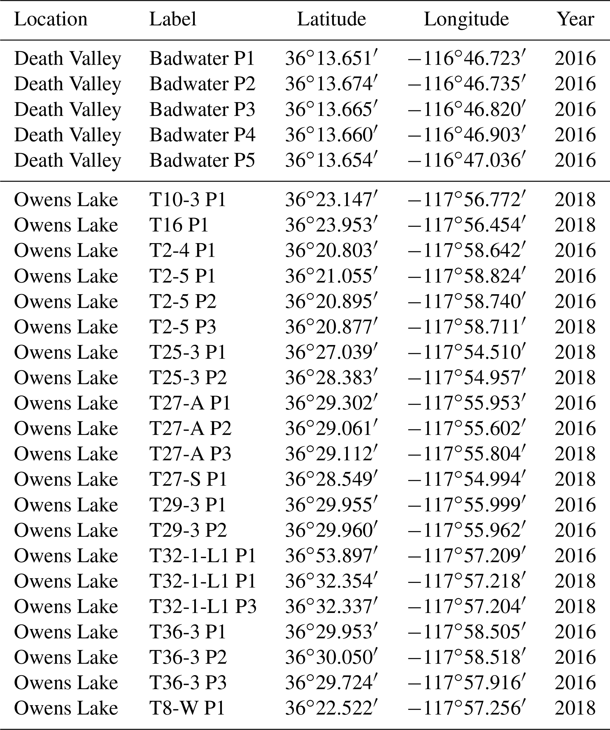
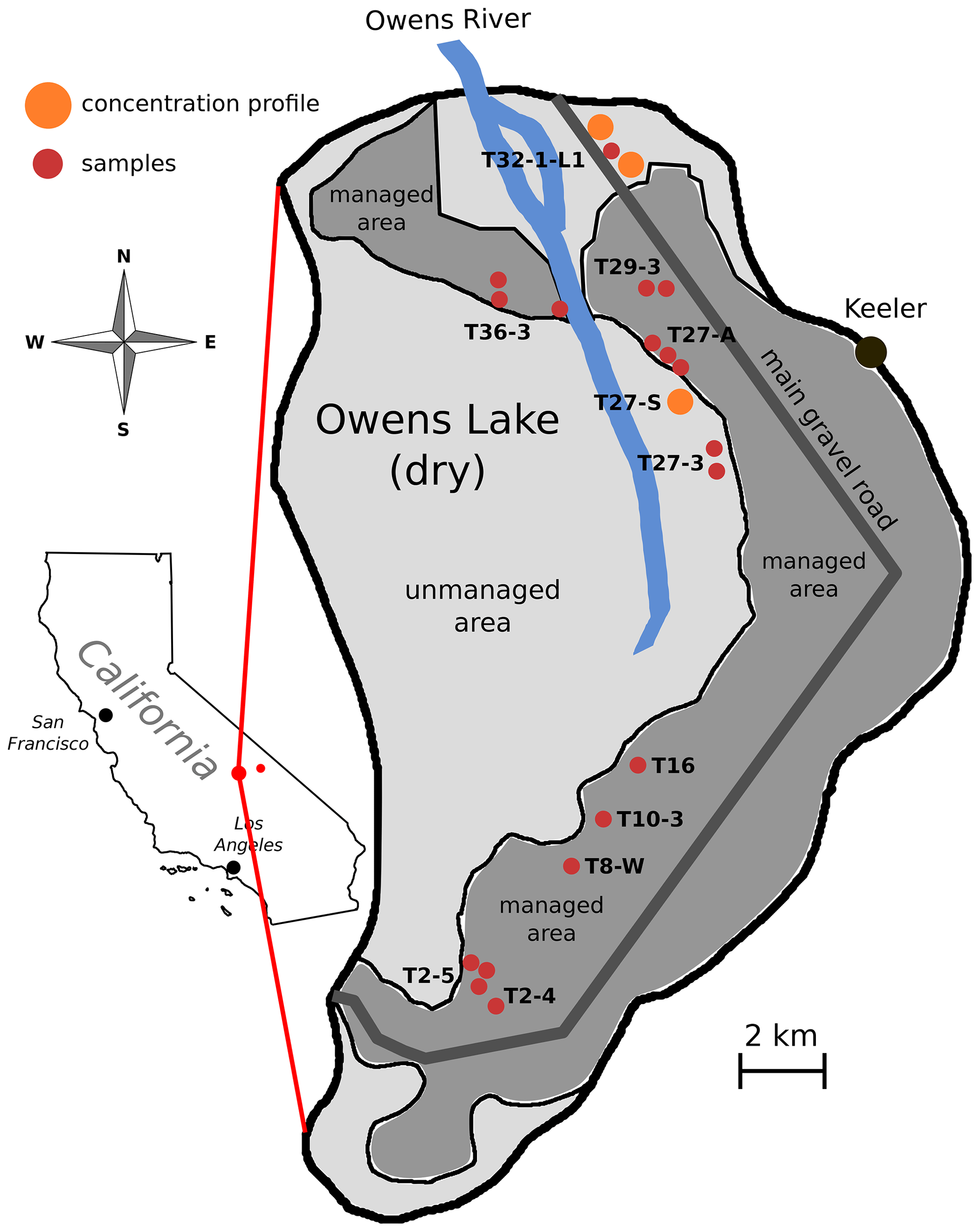
Figure 2 Map of Owens Lake in central California, USA. Sampling sites are indicated by red dots. Sites where we additionally compiled subsurface salinity profiles are indicated by orange dots.

2.1.1 Owens Lake

The Owens Lake basin is bounded by the Sierra Nevada fault zone to the west and the Inyo Mountain fault zone to the east (Hollet et al., 1991). The Owens Valley graben is deepest below Owens Lake: the valley fill reaches a depth of about 2.4 km above the bedrock (Hollet et al., 1991). The valley fill below the dry lake itself consists of moderately to well-sorted layers of sand with grain sizes that range between clay, fine to coarse sand, and gravel (Hollet et al., 1991). The dry lake is framed by alluvial fan deposits. A more detailed description of the geology of Owens Valley is given by Hollet et al. (1991); Sharp and Glazner (1997), and Wilkerson et al. (2007).

All sampling locations at Owens Lake were situated in the area of the alluvial and lacustrine deposits (Hollet et al., 1991). The dry lake is divided into cells on which various dust control measures are implemented such as shallow flooding (Groeneveld and Barz, 2013), vegetation cover (Nicholas and Andy, 1997), gravel cover, and encouraging salt crust growth in brine cells (Groeneveld et al., 2010). We focused our sampling efforts on the brine cells in the north and south of the lake. Study sites at Owens Lake are indicated in the map given in Fig. 2. For these sites we use labels referring to the surface management cells of the dust control project there (LADWP, 2010). These labels refer either to managed cells or to unmanaged areas in the direct vicinity of a managed cell. Labels start with TX-Y, where X is a number, and Y is either a number or one of the letters A, S, and W. The first number refers to water taps (or turn-offs) along the main water pipeline that crosses the lake bed from south to north and which is used to irrigate the managed area. Low tap numbers start in the south, and the numbers generally increase northwards. The second number refers to the Yth management cell connected to the Xth turn-off. The letters A, W, and S refer to addition, west, and south, respectively; they also refer to different subregions branching from the same numbered tap. Following the cell name is the letter P followed by a number which specifies an individual polygon sampled at that site. For example, site label T27-A P3 refers to the third polygon sampled at the addition to the main cell at turn-off 27.

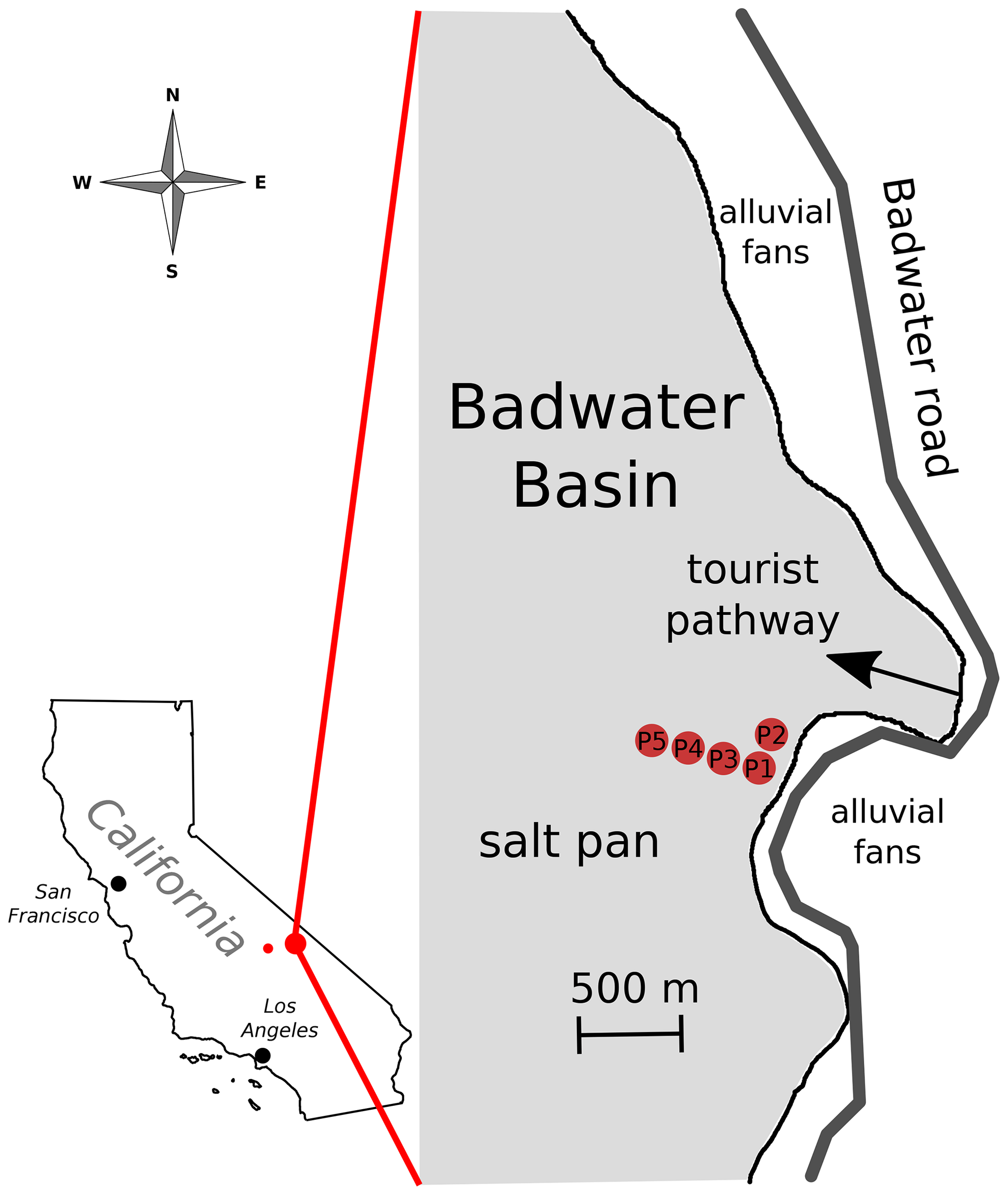
Figure 3 Map of Badwater Basin in Death Valley, central California, USA. Sampling sites are indicated as red dots.

2.1.2 Badwater Basin

Badwater Basin is a geological sink and the lowest point on land in North America, about 86 m below sea level (Hunt et al., 1966). Similar to Owens Lake it is subject to infrequent precipitation events, and evaporation from the playa far outweighs precipitation (Handford, 2003). Groundwater and runoff enter the basin from the surrounding mountains, carrying minerals which accumulate in the basin floor (Hunt et al., 1966). The geology of Badwater Basin and the surrounding Death Valley is described in more detail elsewhere (Hunt et al., 1966; Sharp and Glazner, 1997), but, similar to Owens Lake, it also exhibits a deep bed of unconsolidated valley fill, on which the salt crust rests.

We sampled polygons in an area about 500 m south of the main tourist pathway entering the salt flats from the east. This area, chosen in consultation with park rangers, presented a convenient, typical, and well-developed polygonal crust that was far enough away from the tourist parking to minimise disturbances from other visitors. There, we sampled two polygons about 100 m inwards and parallel to the boundary of the salt flats. Additionally, we sampled three more polygons at distances of about 200, 300, and 400 m inwards from the dry lake edge, respectively, to investigate any systematic effects of distance into the salt pan. All sampling locations are depicted in Fig. 3.

2.2 Measurement protocols, instrumentation, and sample analysis

2.2.1 Subsurface samples

We collected soil samples from below salt polygons using two different methodologies:

1. We dug a trench about 30 cm wide, 2 m long, and 1 m deep and then collected samples from one trench wall, as shown in Fig. 4a.

2. We drew cores with a Dutch gouge auger with a diameter of 50 mm and then collected samples from the cores, as shown in Fig. 4b. This method was used exclusively for wetter sites (water table within 30 cm of surface). The corer was cleaned, rinsed with deionised water, and dried after each use.

For both sampling methodologies, we collected samples from directly below the crust to a depth of up to 1 m. Samples were collected along a grid with a vertical resolution of approximately 0.1 to 0.15 m and a horizontal resolution of 0.15 to 0.3 m. Typically, sampling was done along a line passing through the middle of a polygon, included samples from directly under any bounding ridges, and continued slightly into the two adjacent polygons. The samples had an average volume of approximately 10 mL and were taken using a metal spatula, which was cleaned with distilled water and dried before each use. The samples were a mixture of soil with a grain size of medium sand to clay, pore water, and salt (both dissolved and precipitated). After collection, samples were immediately stored in air-tight containers, which were sealed with Parafilm to prevent the loss of humidity between sample collection and measurement in the laboratory. Soil samples were then returned to the lab for further processing.

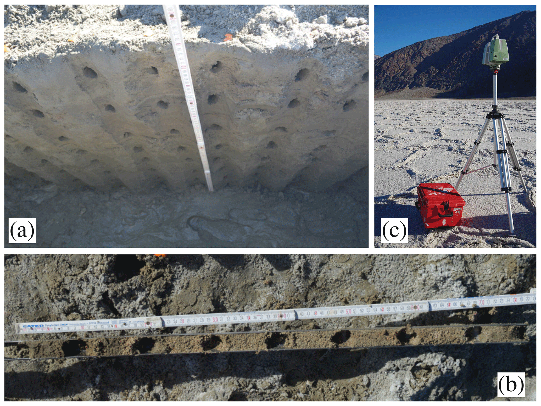
Figure 4 Field methods. (a) Representative trench and sampling positions (holes) at a site at Owens Lake. (b) Dutch gouge auger and sampling positions (holes) at a site at Owens Lake (crust–soil interface is positioned at 0 cm). (c) Terrestrial laser scanner (TLS) set-up at Badwater Basin.

2.2.2 Grain size distributions

We measured the grain size distribution of the soil samples using a Beckman Coulter LS 13 320 laser particle sizer (LPS). As preparation for this, a soil sample would be thoroughly mixed with water but without ultrasound treatment (i.e. we did not attempt to break up grain conglomerates). The resulting soil suspension was then pumped through the laser chamber of the LPS. The LPS measures the diffraction patterns generated as individual grains pass across the laser path, and these signals are converted into grain diameters d_i based on Mie scattering theory (Hahn, 2009) with a real and imaginary component of 1.556 and 0.1, respectively; the underlying diffraction model we used was for quartz. By integrating many such measurements over time, a volume fraction φ_i of grain diameters within a certain range – or bin – is calculated. Results are tabulated as the relative volume of particles within 93 distinct bins of particle diameters, which cover the range from 40 nm to 2000 µm. The upper and lower cut-offs of each bin are given in Lasser and Goehring (2020b) along with these data.

Each grain size distribution measurement is an average of three independent measurements of the same sample. Even though there was no ultrasound treatment before measurement, there was no or only minimal drift towards lower grain sizes due to dissolution of grain conglomerates over the three sequential measurements.

2.2.3 Salinity profiles

For each of the three trench sites (T32-1-L1 P2, T32-1-L1 P3, and T27-S P1) we compiled a cross-sectional salt concentration profile from samples taken from the trench wall, underneath a surface polygon. Samples collected by coring had insufficient sampling resolution to make similar cross-sectional profiles. We discuss the challenges encountered with measuring concentration profiles in more detail in Sect. 2.4. Samples were transported in sealed containers to a laboratory equipped with a high-precision Denver Instrument SI-234 balance with a precision of ±0.1 mg as well as an oven to dry the samples. Gravimetric analysis of salt concentrations was conducted in the following steps:

• The sample was extracted from its storage container into a crystallisation dish, and the initial mass of the mixture of sand, salt, and water was measured.

• The sample was dried in an oven at 80 ^∘C until all moisture had visibly vanished or for at least 24 h, followed by weighing to measure the amount of water that had evaporated from the sample as the difference from the sample mass before drying – i.e. to measure the initial water mass. Care was taken to let the samples cool down completely before weighing because of the temperature sensitivity of the balance.

• The sample was diluted with approximately 50 mL of deionised water followed by sedimentation of the solid sample components for roughly 24 h and careful extraction of the supernatant liquid, which contains the dissolved salt, using a syringe. This step was repeated twice, and the extracted liquid was collected in a separate crystallisation dish.

• The solid and liquid parts of the sample were dried separately in an oven at 80 ^∘C until all moisture had visibly vanished or at least 24 h had passed. For the liquid part, drying sometimes took considerably longer (e.g. a week). Finally, the salt precipitated from the liquid phase and the now salt-free solid residue were individually weighed.

The comparison between the weight of the dry sample, composed of salt and sand, with the weight of the dry sample without the salt gives an indirect measure of the salt content in the sample, whereas the weight of the salt crystallised in the dish gives a direct measure of the salt content. The difference between both weights gives an indication of the reliability of the analysis. If both weights were within the accuracy of the balance, the sample mass was conserved, and the measurement was accepted.

2.2.4 Salt crust and pore water samples

The salt crusts observed at the dry lakes, and especially at Owens Lake, consisted of visually different patches of salt (see Fig. 5). This observation is consistent with the fact that silicates and carbonates have a significantly lower solubility than halite and thenardite and will tend to precipitate first as brine evaporates.

We collected samples from several sites for subsequent chemical and mineral analysis; from each site we collected samples from visibly different regions within the same site.

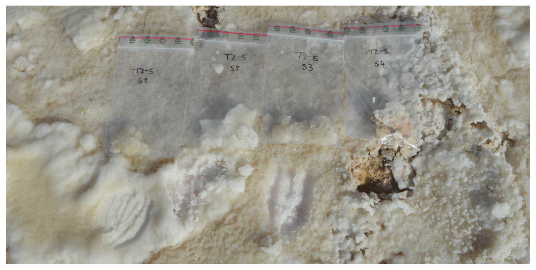
Figure 5 Examples of salt samples collected from the salt crust at site T2-5 P3 at Owens Lake, California.

To collect saline pore water, we used a syringe to draw out the water which gathered in the coring holes. This worked well for the wetter field sites. For the drier sites, where water did not readily gather in the holes, we used a perforated metal rod equipped with a filter and applied a negative pressure to suck water from the pores. In all cases, pore water was taken as close to the water table depth as possible.

2.2.5 X-ray diffraction analysis of crust minerals

To characterise the minerals present in the pore water and surface crust, samples were analysed using quantitative X-ray powder diffraction (XRD). The samples were prepared and analysed according to the following protocol:

• Similar to the procedure for measuring soil composition (Sec. 2.2.3), the total sample mass was first measured. Samples were then dried in an oven at 80 ^∘C for several days, and the sample mass was measured again to determine the mass of the evaporated water.

• Samples were mixed with 10 wt % ZnO (zinc oxide) powder as a known baseline. This is necessary to quantify amorphous components in the sample.

• Samples were milled for 10 min in a McCrown micronising mill to create a fine powder.

• Samples were back-loaded into 27 mm sample holders to preserve a random crystal orientation in the powder.

• Samples were scanned in an X-ray diffractometer, and diffraction patterns were recorded.

• Minerals were identified using the X’Pert HighScore software (PANalytical).

• Mineral composition was quantified based on the Rietveld method using the software AutoQuan (Version 2.7.0.0).

For the XRD analysis we used a Philips X’Pert MPD PW 3040 diffractometer equipped with a PW 3050/10 goniometer, divergence slit of 0.5^∘, anti-scatter slit of 0.5^∘, receiving slit of 0.2 mm, and a secondary graphite monochromator with a 20 mm mask, operating at 40 kV and 30 mA with Cu Kα radiation. The range $\mathrm{2}\mathit{\theta }=\mathrm{4}{}^{\circ }$ to 69.5^∘ was scanned with a step width of 0.02^∘. The counting time was 10 s, and sample spinning was at 1 Hz. This produced measurements of the relative abundance of various salts at each sampled site.

2.2.6 Spectrometry analysis of crust minerals

To confirm the mineral quantifications measured by XRD, we used inductively coupled plasma optical emission spectrometry (ICP-OES) to classify the ions in some of the pore water samples. Minerals from the pore water samples were first dried as described in Sect. 2.2.5. The residual salts were then redissolved in a known amount of water for measurement with ICP-OES.

All samples were analysed by an Agilent 5100 VDV ICP-OES. Ba, Ca, K, Na, and Sr were measured in radial view mode and all other ions in axial view mode. Standardisation was done by using five matrix-matched multi-element calibration solutions and a blank solution. All solutions contained HNO₃ at a concentration of 1.56 M. The mean of six blank measurements was subtracted from each measurement. The detection limit was calculated as 3σD_BLANK, where D_BLANK is the blank measurement. Repeatability of the ICP-OES measurements is about 1 %, with a calibration error of <5 %. Therefore, we assume a measurement accuracy of 5 %.

2.2.7 Water density

To obtain a measurement of the water density, pore water samples were analysed in the laboratory using an Anton Paar DMA 4500 vibrating-tube densitometer with a measurement accuracy of $\mathrm{5}\times {\mathrm{10}}^{-\mathrm{4}}$g/cm³. For each sample, at least two measurements were performed.

2.2.8 Temperature and relative-humidity records

To characterise the environmental conditions at the field sites and how the surface crust introduces heterogeneity into these conditions, we embedded sensors into the crust and tracked their temperature and relative humidity over several days. Half of the sensors were placed inside hollow salt ridges (tepee structures) by carefully removing a small section of the salt crust at the ridge, inserting the sensor into the hollow space inside the ridge, and then putting the removed crust part back in place. The other sensors were embedded in the flat section of the salt crust in the middle of salt polygons. For these sensors, a small hole was dug into the crust, and broken-up salt crystals were removed. The sensor was placed inside and then covered by the broken-up salt crystals. The measurements from within ridges can be compared to measurements of temperature and relative humidity recorded from sensors placed in the centres of polygons. For temperature and relative-humidity measurements, we used HiTemp140 and RHTemp1000IS data loggers, which measured temperatures and relative humidity every Δt=60 s or Δt=120 s with a precision of ±0.01 ^∘C and ±0.1 %, respectively. The factory calibration was used for all sensors. Although we did not cross-reference the sensors explicitly, the values from different sensors showed consistent values under similar conditions both indoors and outdoors.

2.2.9 Surface scans using a terrestrial laser scanner (TLS)

To characterise the surface crust patterns, we recorded high-resolution, three-dimensional point clouds of the surface relief using a Leica P20 terrestrial laser scanner (TLS). From these, we extracted a characteristic pattern wavelength λ and ridge height h.

The scanner was positioned at a height of at least 2 m above the crust (see Fig. 4c), and it then recorded the surface relief in a circular sweep from a distance of about 1 m from the scanner up to a distance of about 50 m. In principle the scanner can record the surface relief at even larger distances but becomes increasingly prone to occlusion by surface features which lie in the path of the scanning beam. Additionally, the resolution of the scan decreases with distance from the scanner as the number of points measured along a circle with a given radius is fixed, even if the radius increases. Conversely, the resolution is highest in the direct vicinity of the scanner. Therefore we typically positioned the scanner not more than 10 m away from the polygon we intended to sample in order to record the pattern around the focal polygon with the highest possible accuracy.

At some sites it was possible to position the scanner on one of the gravel roads next to the site and therefore increase the vertical distance of the scanner to the crust to about 5 m. This was desirable as it reduced occlusion at larger scanning distances. At such sites we aimed to position the scanner such that the focal polygon was in the centre of the scanned area, which was a half-circle bounded by the gravel road. We aimed to scan each site we sampled before beginning the sampling procedure (i.e. before disturbing the naturally grown crust).

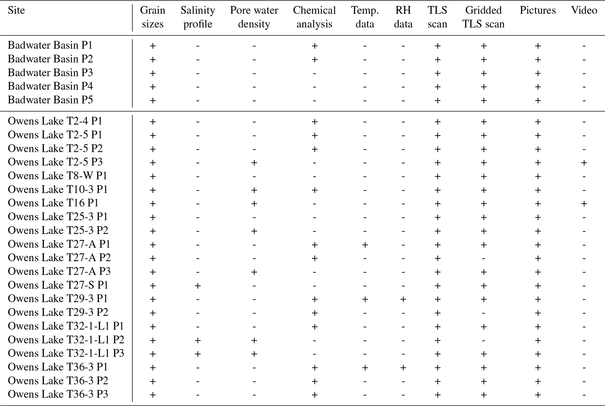
Table 2 Availability of data sets for each of the 5 field sites at Badwater Basin and the 21 field sites at Owens Lake. Columns indicate data sets for grain size distributions (Lasser and Goehring, 2020b), salt concentration profiles, pore water density measurements (Lasser and Goehring, 2020a), chemical analysis of the pore water and salt crust components (Lasser and Karius, 2020), temperature and relative-humidity (RH) time series (Nield et al., 2020a), raw and gridded TLS surface scan data (Nield et al., 2020b), and pictures and time lapse videos of the field sites (Lasser et al., 2020a). All data sets are available at PANGAEA.

2.2.10 TLS data processing

Scans acquired by the TLS were subject to several post-processing steps following Nield et al. (2013) and described in detail there. The main steps included (1) extraction of a 10 m×10 m area of surface relief from the scan, including the sampled polygon at each site; (2) gridding of the data points into regular Cartesian coordinates using a nearest-neighbour algorithm implemented in MATLAB; and (3) subtracting out the average background height of the surface. Due to the gridding into Cartesian coordinates, the best resolution of the surface relief in the processed data is 10 mm in the horizontal and 0.3 mm in the vertical direction.

Table 3 Structure of the grain size analysis data sets at PANGEA (Lasser and Goehring, 2020b). Column names identify the depth at which each sample was collected; a lower (10th percentile), median, and upper (90th percentile) representative value of the grain size distribution; a general soil classification based on the most ubiquitous grain size range (following Chesworth, 2008); and the weight percentage of water in the soil sample. Column names also identify the lower channel diameter of the laser particle analyser (µm), the differential volume recorded in the respective channel, and the differential volume minus (plus) two standard deviations. Additionally, the middle and upper channel diameter (µm), the middle channel diameter in the Krumbein ϕ scale (Krumbein, 1934), and the cumulated differential volume are reported.

2.2.11 Time lapse photography

To investigate the salt crust growth process, we recorded time lapse images of crusts at Owens Lake in spring 2018. We installed three cameras (Ltl Acorn 5210A Trail Camera 940NM) at different sites. All cameras were positioned in areas where shallow flooding was implemented as a dust control measure and which were wet during our visit. We choose these sites since they promised to show active crust growth as temperatures increased and water evaporated during the course of the year.

We installed the cameras on tripods at a height of 1.5 m above the crust and secured them with rocks against strong winds. The battery-powered cameras recorded an image of a crust section of about 4 m ×6 m in front of them every 30 min, from 16 January to 7 July 2018. We placed 0.1 m ×0.1 m white, grey, and black tiles in the cameras' fields of view to allow us to calibrate the white balance and to act as a scale bar. Images were recorded with a resolution of 12 megapixels. Cameras were equipped with an infrared flash, which allowed them to record images during the night as well. Cameras were also equipped with a temperature sensor, which recorded temperature with a precision of $\pm \mathrm{1}{}^{\circ }$C. Since a camera's temperature sensor is embedded in its black casing, it overestimates temperatures during sunny days as the casing absorbs radiation and heats up. Date, time, and temperature are encoded at the bottom of the recorded images.

Once installed, one camera completely failed to record any images. Of the remaining two cameras, about two-thirds of the images recorded by the cameras either failed to record completely or contained substantial digital artefacts. This may be due to the rather harsh climate and other conditions at Owens Lake. To compare images with comparable lighting conditions, we handpicked images that recorded properly for every day shortly after sunrise and stitched them into a movie. Cameras stayed stationary during the whole period of recording, and no realignment of images was necessary.

Table 4 Positions of the polygon ridges at the trench sites for which subsurface salinity profiles were collected, relative to the start of the sampling transect.

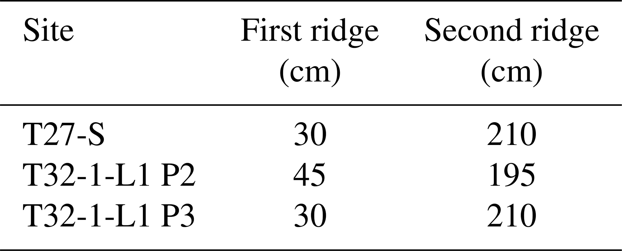
Table 5 Structure of the subsurface salinity profile data sets at PANGEA (Lasser and Goehring, 2020a). The data contain sample labels; the vertical (Z) and horizontal (X) position of each sample along the survey; and the masses of water, sand, and salt (measured by two methods) in those samples. See Sect. 2.2.3 for details of analysis methods.

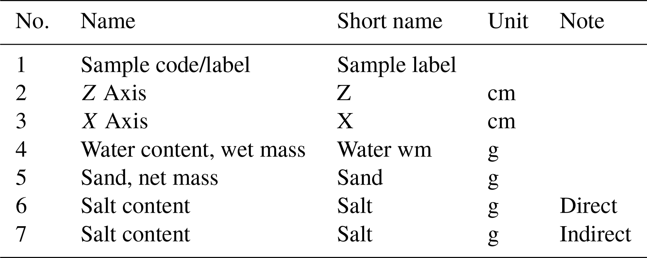
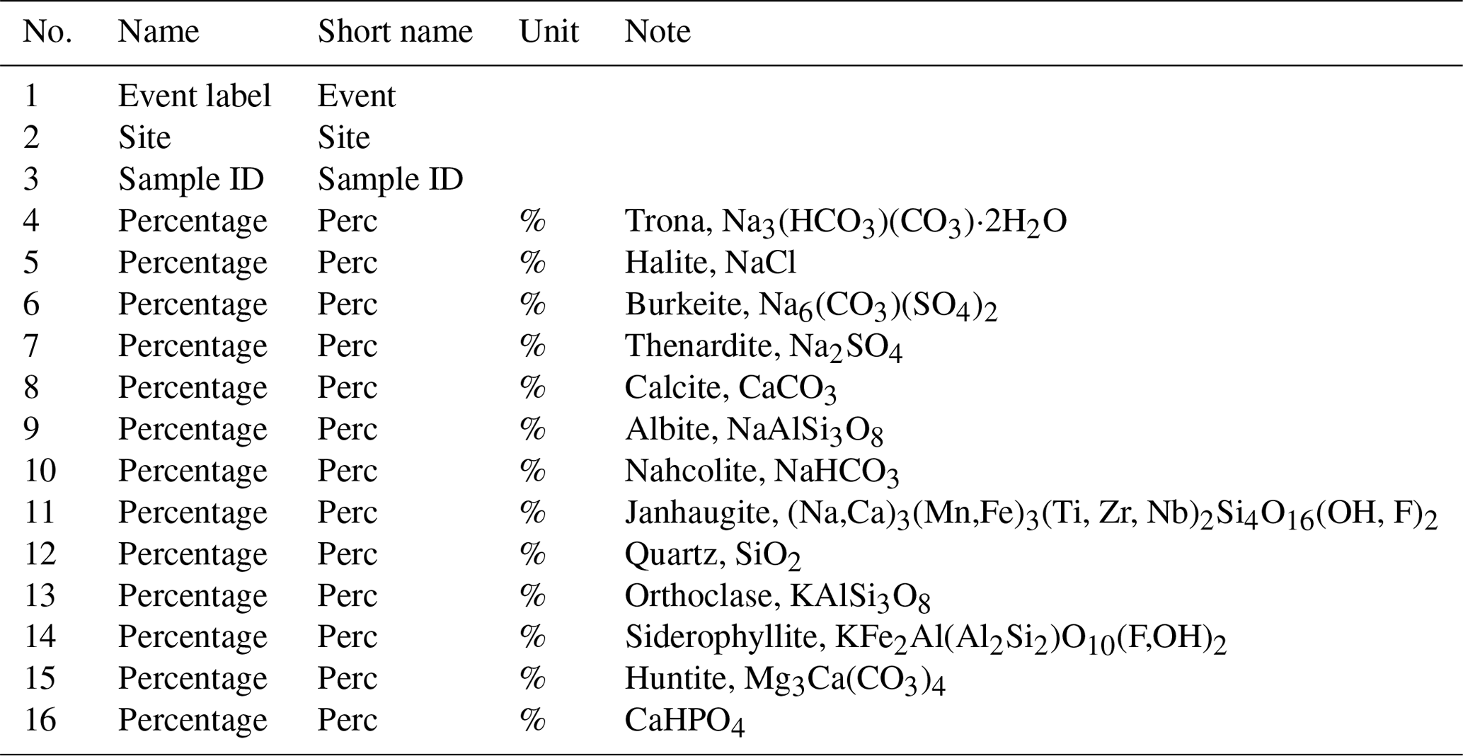
Table 6 Structure of the salt crust salt mineral characterisation via quantitative X-ray diffraction data set at PANGEA (Lasser and Karius, 2020). The data consist of site and sample IDs and the weight percentages of various salts within each sample.

2.2.12 Pictures

During the two field trips, various pictures of the field sites, the salt crust, and the sampling process were recorded using several different cameras. From these images, a subset of images was selected to characterise each site.

2.3 Data provenance, structure, and availability

An overview of all the available data is given in Table 2, indicating which type of data was collected and published from each site.

2.3.1 Grain size distributions

Data of grain size distributions are deposited at PANGAEA for 21 sites at Owens Lake and 5 sites at Badwater Basin (Lasser and Goehring, 2020b). For each site, grain size distributions were measured for samples taken at different depths (for methods see Sect. 2.2.2). The overall soil composition is given as the dominant sample component following the Udden–Wentworth scale (Chesworth, 2008). The structure of the data sets is shown in Table 3.

2.3.2 Cross-sectional salinity profiles

Data of subsurface salinity distributions are available at PANGAEA for the three trench sites at Owens Lake (Lasser and Goehring, 2020a). The lateral position of a sample refers to the distance from the first sample taken along a line that bisects the main sampled polygon and extends slightly into the two adjacent polygons. The positions of the salt ridges at the surface for the sites are given in Table 4.

The data were collected during a field campaign in January 2018. Gaps in the data are due to either contamination of samples with surface salt or loss of samples during the destructive analysis process. The structure of the data sets is shown in Table 5.

2.3.3 X-ray diffraction data

Data of the composition of the salt crust analysed via quantitative X-ray diffraction are available at PANGAEA for 10 samples from two sites at Owens Lake (Lasser and Karius, 2020). Samples were collected in 2016. The structure of the data sets is shown in Table 6.

Table 7 Structure of the pore water ion characterisation via ICP-OES data set at PANGEA (Lasser and Karius, 2020). The data give sample locations and the concentrations of various ions dissolved in the water samples.

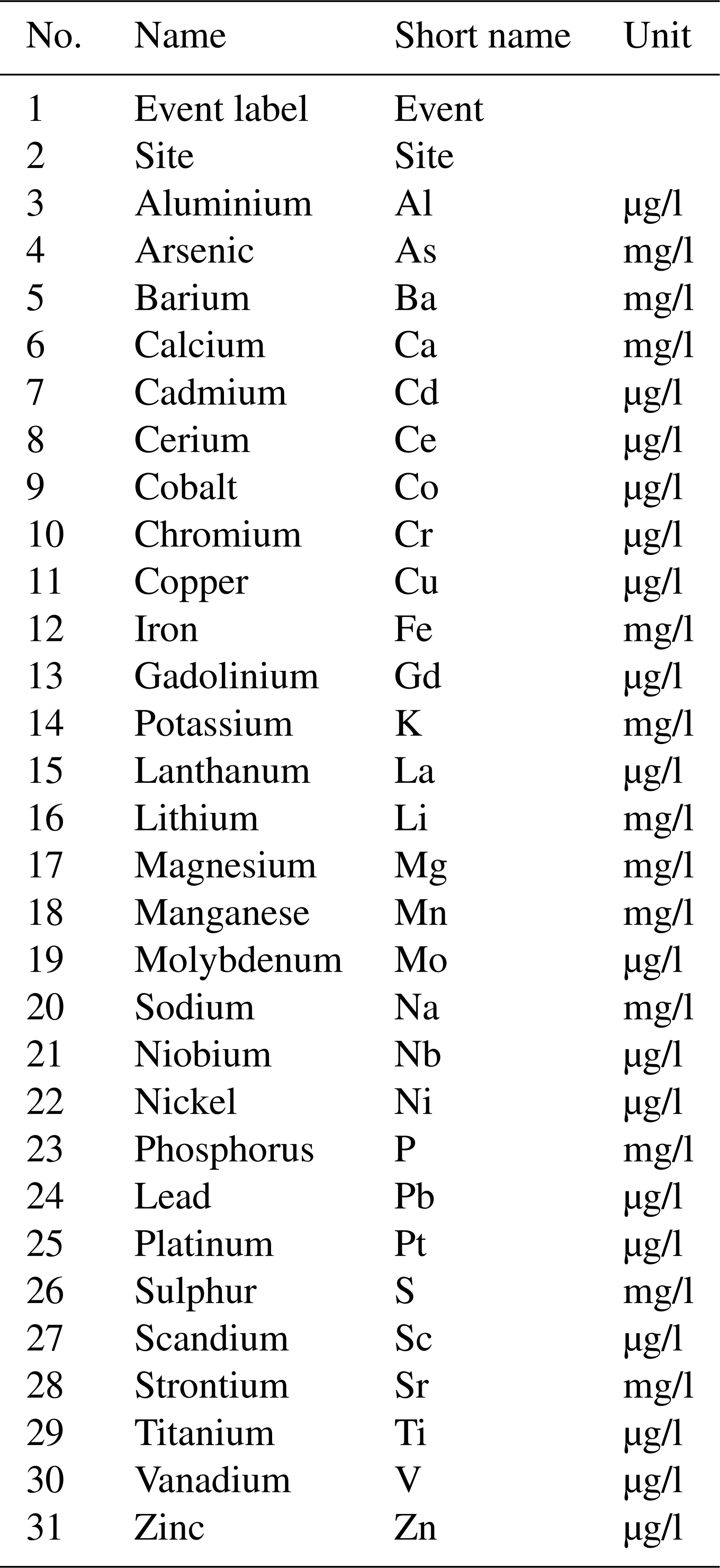
Table 8 Structure of the pore water density data sets at PANGEA (Lasser and Goehring, 2020a). The data include site and sample labels, the depth of each water sample (typically at the water table height), and its horizontal location along the transect as well as all individual density measurements and the averages and standard deviations for each sample.

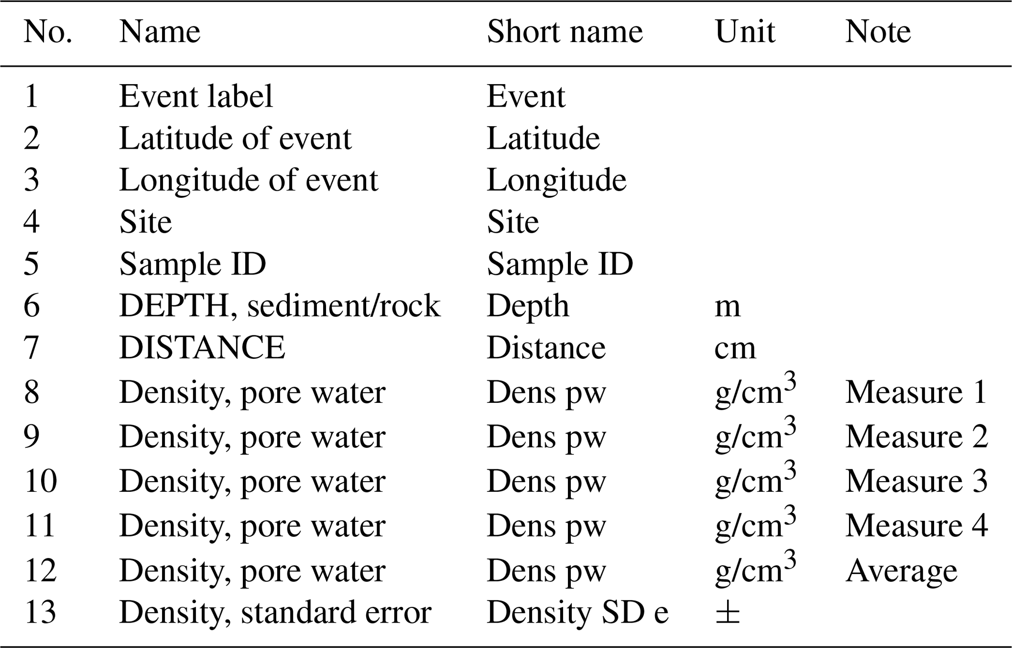
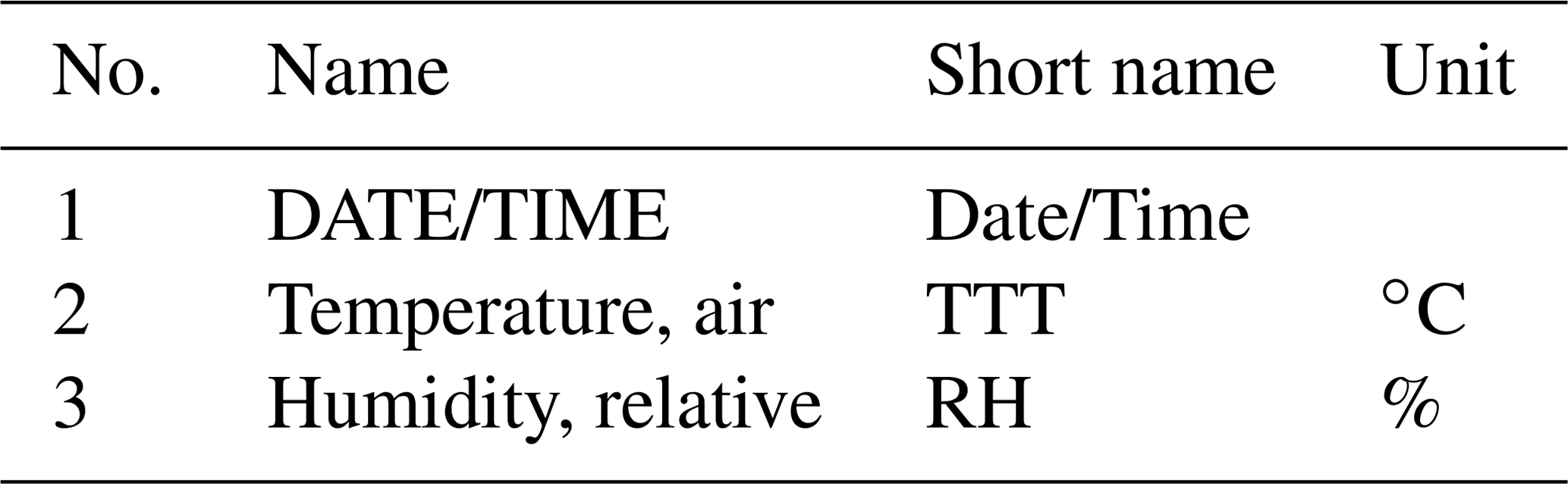
Table 9 Structure of temperature and relative-humidity data sets at PANGEA (Nield et al., 2020a). Data are taken at the ridges and polygon centres of three sites every 2 min from 25 November to 2 December 2016.

2.3.4 Spectrometry data

Data of the composition of the pore water analysed via ICP-OES are available at PANGAEA for 10 sites at Owens Lake and two sites at Badwater Basin (Lasser and Karius, 2020). Samples were collected during 2016. The ICP-OES analysed for the ions of 29 distinct elements in solution. The structure of the data sets is shown in Table 7.

2.3.5 Water density data

Data of pore water density are available at PANGAEA for seven sites at Owens Lake (Lasser and Goehring, 2020a). Individual measurements of densities are reported, along with averages and standard deviations for all measurements on individual samples. In addition to several replication measurements on particular samples, the data set also contains five “validation” samples for site T16 P1. These validation samples were independently collected, stored, transported, and measured but drawn from the same sample site. Therefore they represent a validation of a sample that was duplicated at the point of sample collection rather than at the point of measurement (indicated by a shared sample ID in the data set). The structure of the data sets is shown in Table 8.

2.3.6 Temperature and relative-humidity recordings

Data of the temperature and relative-humidity recordings are available at PANGAEA for three sites at Owens Lake (Nield et al., 2020a). The data were collected from 25 November to 2 December 2016. The structure of the data sets is shown in Table 9. Note that not all tables contain a humidity column since some sensors were only able to record temperature. We truncated the recorded data at the beginning and end to remove data points corresponding to a transient phase directly after putting the sensors in place and after removing them, respectively.

2.3.7 Surface scans

Raw 3D point clouds recorded with a TLS are available at PANGAEA for all sites at Owens Lake and Badwater Basin. The raw point cloud data sets each contain a list of points containing coordinates in the format of (x position, y position, elevation). These data are georeferenced and give easting (x position) and northing (y position) within the US National Grid (USNG). For Owens Lake, these positions are relative to grid zone and square 11S MA, whereas locations at Badwater Basin are relative to 11S NA. Elevations are referenced to the WGS 84 geoid.

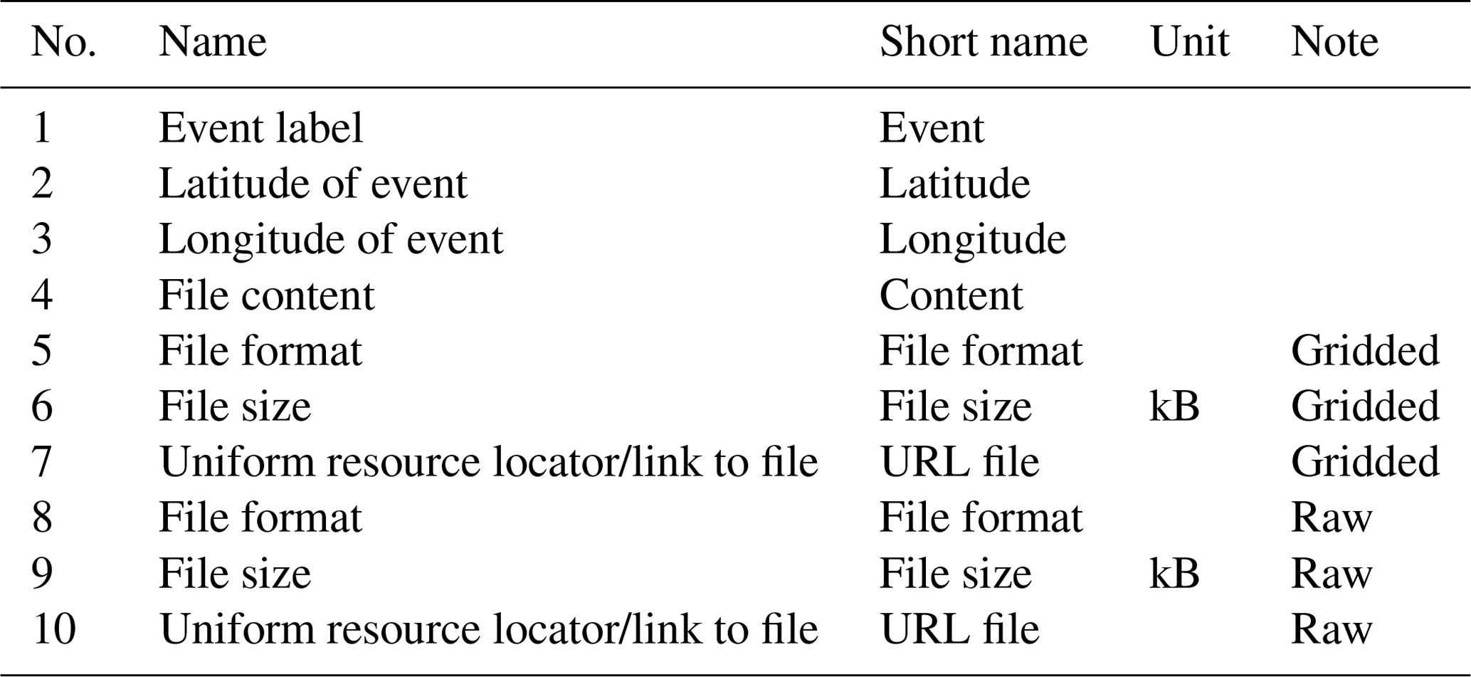
Gridded subsets of the point clouds are available for all sites at Badwater Basin and for 18 sites at Owens Lake (Nield et al., 2020b), as listed in Table 2. These data sets are matrices, where each entry represents an elevation. Points are regularly spaced with a resolution of $\mathrm{\Delta }x=\mathrm{\Delta }y=\mathrm{0.01}$m. Raw and gridded data are stored as space-separated .txt and .xyz files and can be read for example using the numpy.loadtxt() method in Python or imported into Excel as a space-delimited table of values.

The structure of the tables further detailing both types of TLS data is shown in Table 10. All positions and elevations are reported in metres.

Table 10 Structure of the surface scan data set collection of raw point clouds and gridded subsets at PANGEA (Nield et al., 2020b). For each scan there is also an associated file containing a full 3D point cloud of the surface scan, with links embedded in the data table.

2.3.8 Pictures

Pictures are available at PANGAEA for all 21 sites at Owens Lake and 5 sites at Badwater Basin (Lasser et al., 2020a). The data set also contains two time lapse videos of sites T16 P1 and T2-5 P3 at Owens Lake. The set of images for each field site contains the following:

• three images of the field site and its general surroundings;

• up to three images of single polygons with a scale bar at the field site;

• one image of the sampled polygon with an indication of the sampling positions (either small holes in the crust or orange markers);

• one image of the sampled core; and

• up to 8 images of salt crust features.

The sizes of various items included for scale in the images are given in Table 11. The structure of the data set collection is shown in Table 12.

Table 11 Sizes of various items included for scale in images from the data set given by Lasser et al. (2020a).

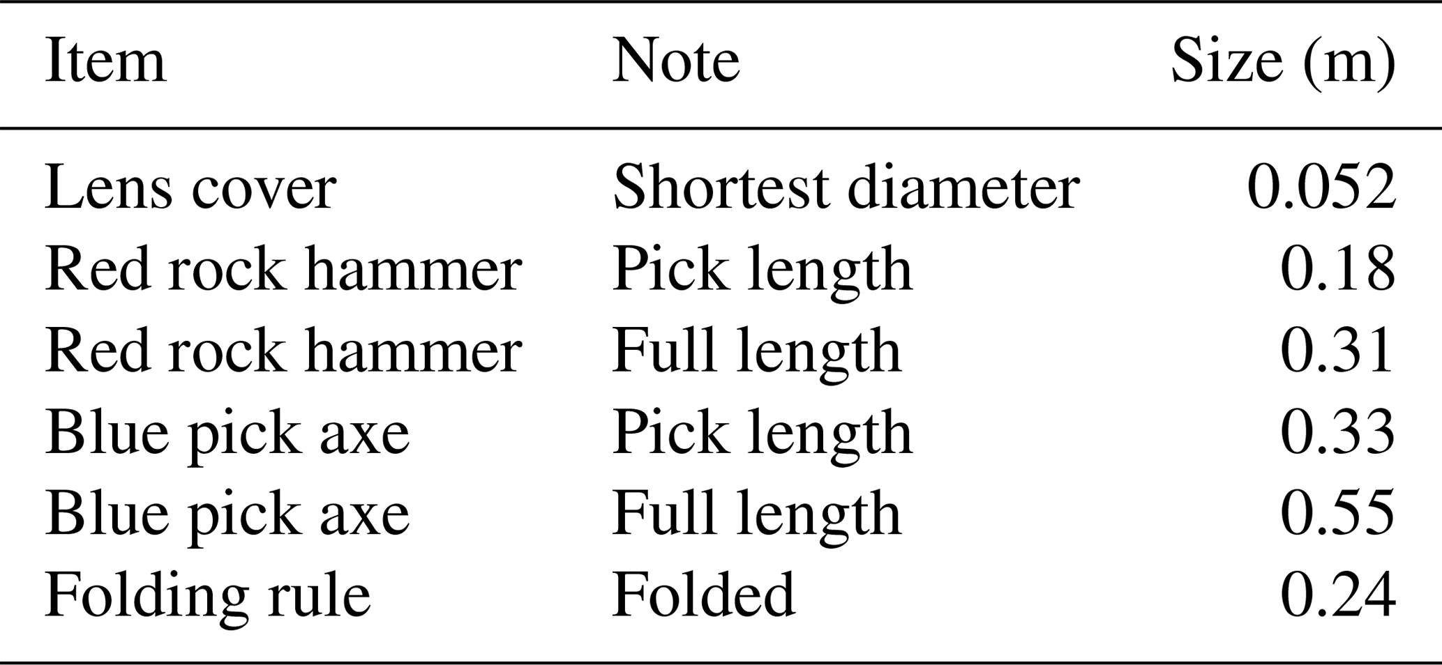
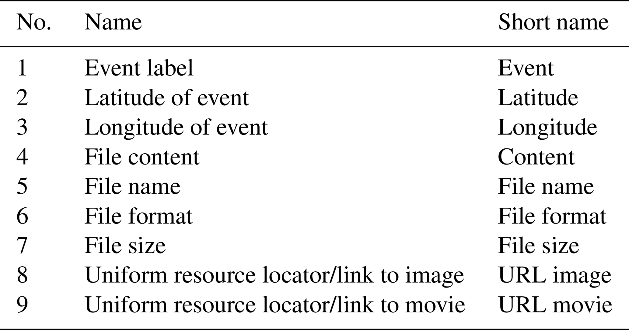
Table 12 Structure of the image and video collection of field sites at PANGEA (Lasser et al., 2020a). The data table contains links to the individual images and time lapse movies.

2.4 Results

Here we present sample data from each of the different data sets in order to illustrate the kind and quality of information contained in them.

2.4.1 Grain size distributions

Exemplary grain size distributions are shown in Fig. 6 for Owens Lake (Fig. 6a) and Badwater Basin (Fig. 6b). These show how the distribution of particle sizes changes with depth at a representative site from each lake. Depending on the site, grain size distributions often show a pronounced layering of the soil, featuring widely varying multimodal grain size distributions. This is indicative of a phased sand deposition process (Earle, 2015, p. 361) and consistent with the history of flooding following heavy rainfall at both Owens Lake and Badwater Basin.

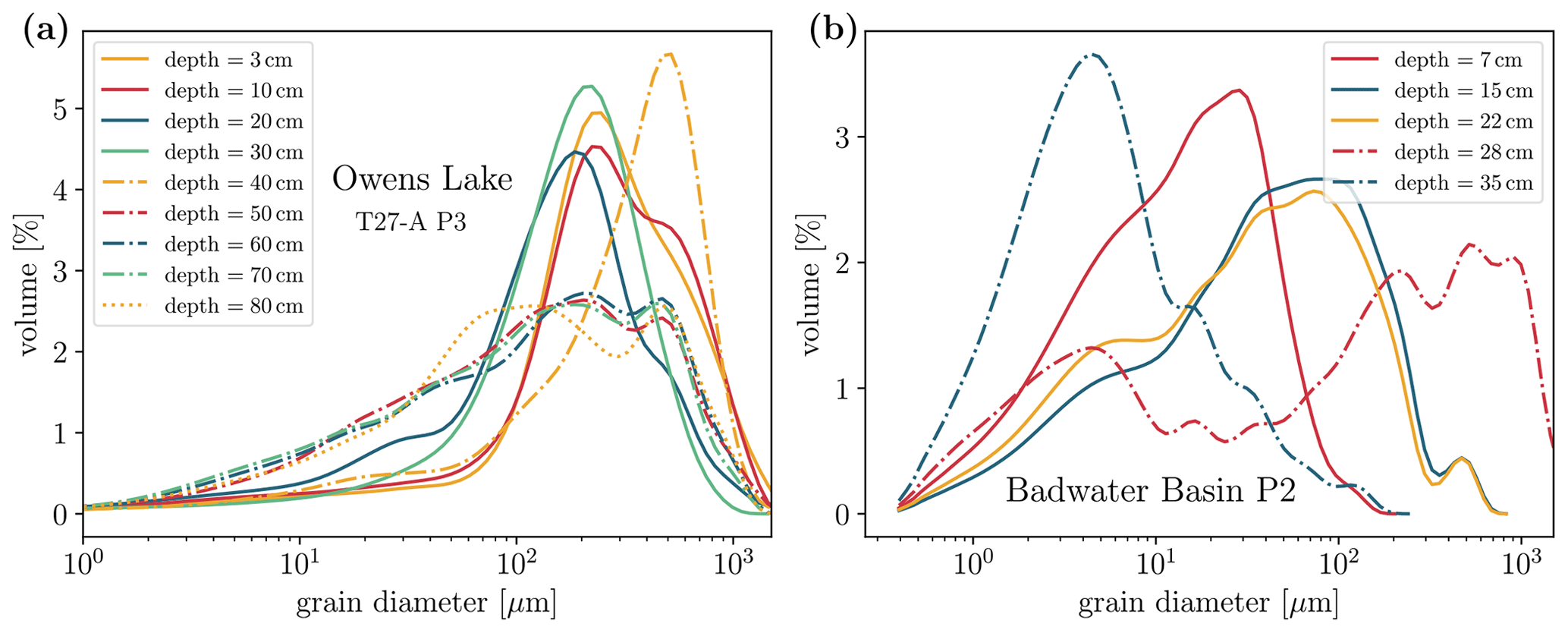
Figure 6 Exemplary grain size (diameter) profiles for (a) site T27-A P3 at Owens Lake and (b) site Badwater Basin P2.

2.4.2 Salinity profiles

As mentioned in Sect. 2.2.3, we used two different methodologies during sample collection: at drier sites (with a water table at approximately 0.7 m) we dug trenches, whereas at wetter sites with a water table nearer to the salt crust (typically at a depth of 0 to 0.3 m) we extracted soil cores using a Dutch gouge auger. The sampling from trenches yielded much more reliable results than the sampling from cores. Consequently, only samples from trench sites were used to compile salinity profiles. One example of a salinity profile compiled from samples extracted from a trench is given in Fig. 7.

Analysis of many of the wet sites showed that the coring method introduced significant noise into the salt content measurements. We identified two main sources of this noise. Firstly, salt crystals (often from the crust) could be pushed into the soil by the corer and subsequently positioned away from their original depths. Even small displaced salt crystals are enough to considerably disturb the measurements of salt content. Secondly, water from close to the surface and presumably with a high salt concentration was often seen to be running down the corer after we pulled it out of the ground. We tried to prevent contamination by sampling with the core laid out horizontally and by removing an outer layer of approximately 5 mm from the surface of the core prior to sample collection. Nevertheless, especially for high-permeability soils, the core was likely contaminated by brine to some degree.

Additionally, during the 2016 field campaign, we sampled the soil with a lower horizontal resolution. As a consequence, results from sites where we used the corer and where we collected samples with a horizontal resolution lower than Δx=0.2 m were not used for the analysis of concentration gradients.

We also performed a reproducibility trial of the salinity profiles by collecting replicate samples at one site where samples were collected via the corer. The maximum deviation in salinity between the samples collected right next to each other was 5.7 wt %. Excluding the shallowest two rows of samples (where contamination from surface crust pieces is likely), the maximum deviation is about 2.5 wt % and the mean deviation is about 1 wt %.

During the laboratory analysis of the salt contained in the samples, a small number of samples were contaminated or lost due to mistakes in the dilution process or broken crystallisation dishes. Consequently, these data points are missing from either the direct or indirect measurement column in the data set. Otherwise, agreement between the direct and indirect measurements for all three sites is very high, with R²=0.98 (p<0.001) for site T27-S P1, R²=0.96 (p<0.001) for site T32-1-L1 P2, and R²=0.93 (p<0.001) for site T32-1-L1 P3.

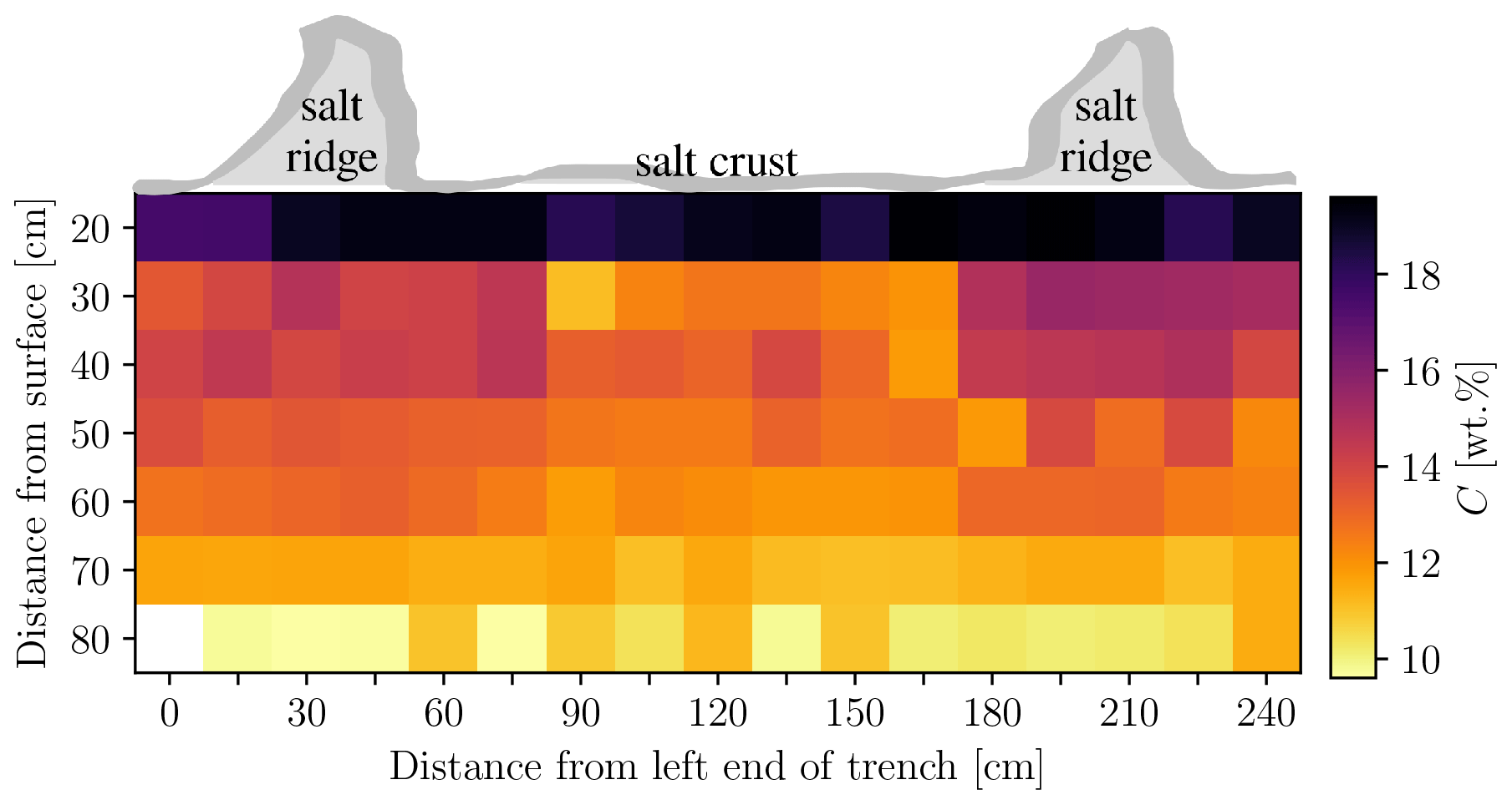
Figure 7 Salinity profile compiled from samples taken at site Owens Lake T27-S P1 in January 2018. The colour code indicates the salt concentration C in wt %.

2.4.3 Chemical analysis

The most abundant salts found in the different crust samples collected from two sites at Owens Lake are listed in Table 13. The samples, taken from visually distinct patches of salt that were nonetheless near to each other, show different compositions. This presumably reflects how the various salts in solution will start to crystallise at different times in the brine evaporation process.

At Owens Lake the analysis of pore water ions via ICP-OES is dominated by sodium, sulphur, and potassium (in descending levels of significance) but also shows notably high levels of arsenic, of up to 150 µg/l. This is consistent with other reports of arsenic found in the salt crust (Ryu et al., 2002; Gill et al., 2002).

Table 13 List of the most and second-most abundant salt species in crust samples taken at sites T2-5 and T10-3. The full data set is available in Lasser and Karius (2020).

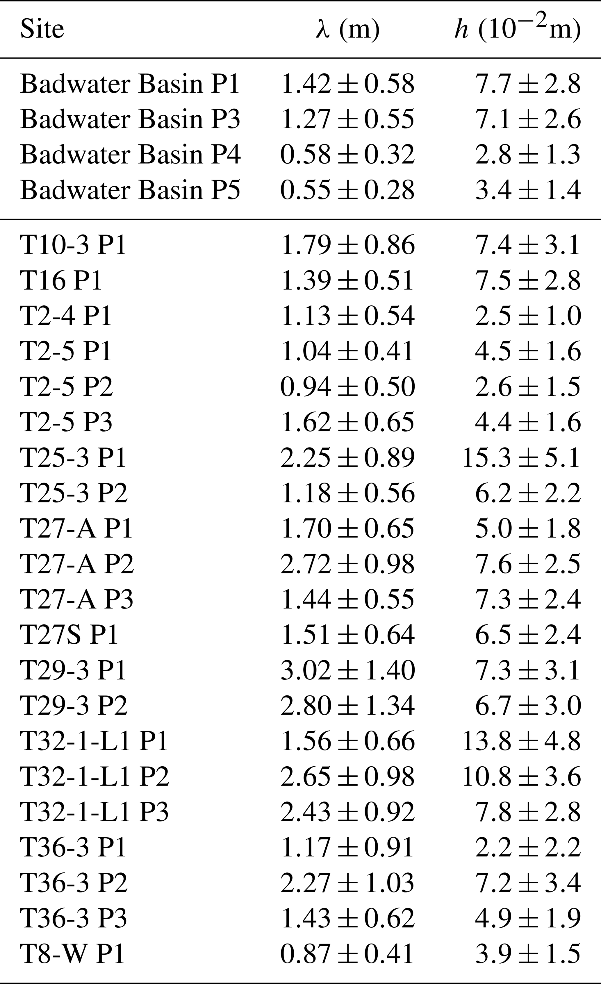
Table 14 Average pattern wavelengths (λ) and ridge heights (h) calculated from surface scans of salt pans showing polygonal shapes. Ranges indicate the standard deviation of each set of measurements.

2.4.4 Water density

Measurements of the density of water samples collected from different depths allow for a reliable quantification of the background salinity at Owens Lake. A comparison between the background salinity and surface salinity then allows for an estimation of the buoyancy forces that the more saline and therefore heavier water at the surface is subjected to. Water samples collected from at the surface (or just under the crust) typically show density values of approximately 1.21 g/mL, whereas at a depth of about 0.9 m the pore water density is approximately 1.05 g/mL. This is consistent with water density measurements performed by Tyler et al. (1997). Both Owens Lake and Badwater Basin show a salinity distribution that should allow for the convective overturning of their pore water (Wooding et al., 1997; Lasser et al., 2019).

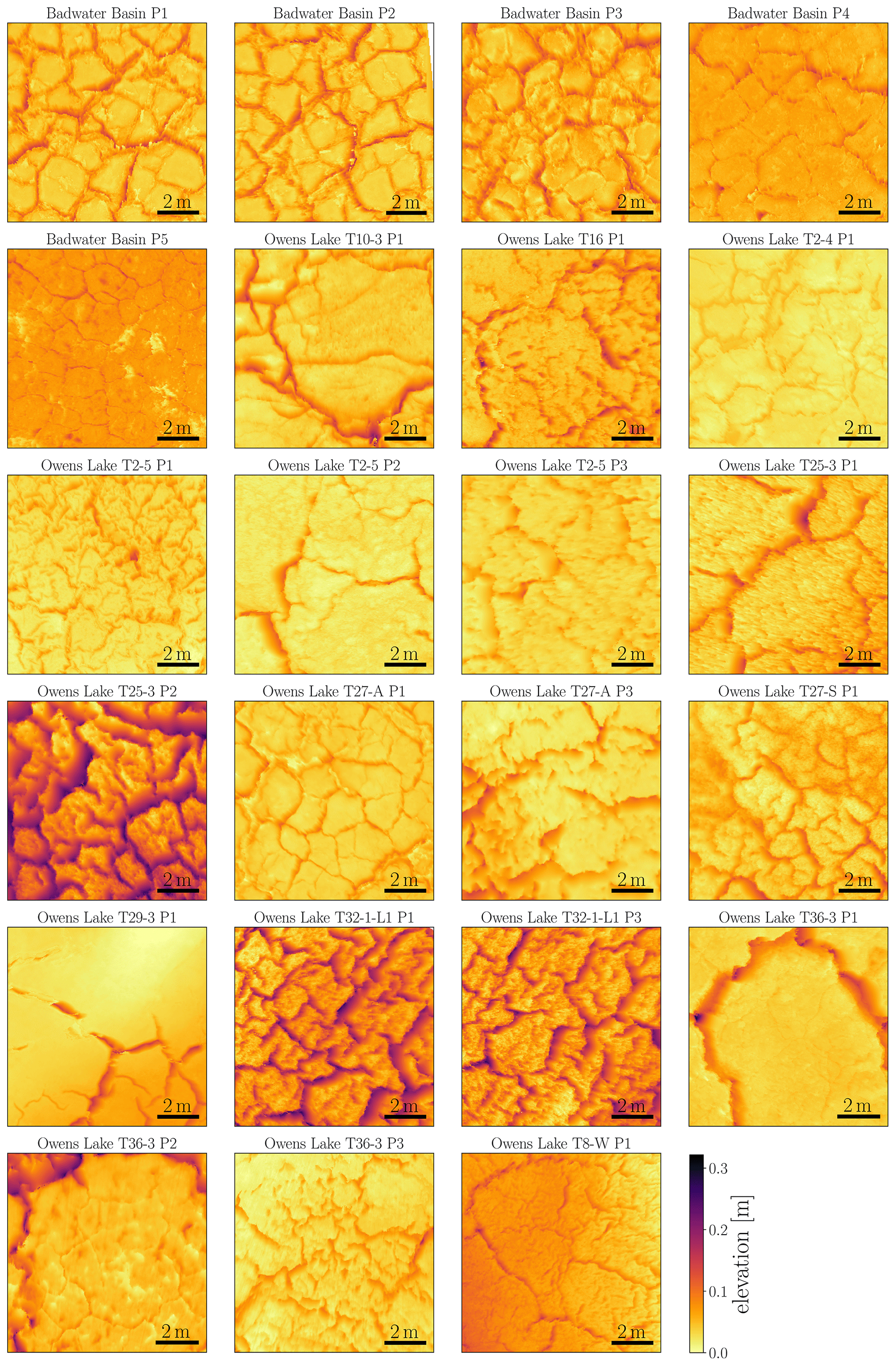
Figure 8 Gridded subsets of the surface relief measured by TLS at sites at Owens Lake and Badwater Basin. The elevation reflects the surface height above the lowest point in each relief.

2.4.5 Surface scans

Scans of salt pan surfaces, using a high-resolution terrestrial laser scanner, allow for a quantification of the pattern dimensions. Gridded subsets consisting of the three-dimensional point clouds of various ∼10 m × 10 m areas are shown in Fig. 8. The average pattern wavelengths, λ, and average ridge heights, h, for each site were calculated from the gridded scans and are given in Table 14. Uncertainties for λ and h are given as the standard deviations of the measured pattern wavelength and height in the gridded subset, respectively. Values for the pattern wavelength consistently lie in the range of 0.5 to 3 m. Furthermore, the pattern wavelength is weakly but positively correlated with polygon height (R²=0.31, p=0.004). The values for the wavelength can also be compared to models of subsurface convective motion (see for example Lasser et al., 2019).

2.4.6 Videos

The two videos that were successfully compiled from time lapse photography at sites Owens Lake T16 P1 and Owens Lake T2-5 P3 show the growth of the salt crust from a flooded configuration. Growth starts as soon as the water table sinks below the crust surface, in late March and early April. Ridges seem to preferentially grow in locations where ridges were present before the flooding. From the videos, salt ridge growth of about 30–50 mm over the course of 20 d can be inferred, i.e. a rate of about 2 mm/d (see video from site Owens Lake T16 P1, lower right corner), which is similar to the growth rates observed for salt pans in Botswana (Nield et al., 2015).

3 Summary

Six data sets were presented which characterise the surface, subsurface, and environmental conditions of two dry salt lakes – Owens Lake and Badwater Basin – in central California. The data sets include grain size distribution measurements of sand samples taken at these locations (Lasser and Goehring, 2020b), subsurface cross-sectional salt concentration profiles and pore water density measurements (Lasser and Goehring, 2020a), a chemical characterisation of the various salts present in the salt crust and pore water (Lasser and Karius, 2020), temperature and relative-humidity measurements from within salt ridges and polygon centres (Nield et al., 2020a), high-resolution surface scans measured using a terrestrial laser scanner (Nield et al., 2020b), and images characterising the field sites and time lapse videos capturing the growth of salt polygons (Lasser et al., 2020a).

Grain size distributions, surface scans, and images cover all 26 sites at Badwater Basin and Owens Lake that were visited and allow for an in-depth characterisation of surface and subsurface conditions at these salt pans. Temperature and relative-humidity recordings are only available for three sites at Owens Lake but allow for an estimation of the impact of the presence of salt ridges on temperature and humidity and therefore evaporation of water from the crust. Videos were compiled at two sites at Owens Lake and are direct evidence of salt ridges growing on a very short timescale. The analysis of salt species only covers two sites at Badwater Basin and six at Owens Lake. Nevertheless it is to be expected that other sites in the area have a similar mineral composition since they are connected to the same groundwater reservoirs.

For future research, the environmental conditions at the salt polygons and inside the salt ridges could be better described since they are closely linked to evaporative processes in these landscapes. Evaporation is important both for the water and energy balance of salt pans and as a driver of potential dynamical processes below the crust. Measurements of temperature and relative humidity could also be accompanied by direct measurements of the evaporation rate.

Furthermore, properties of the salt crust itself, such as crust thickness, would likely be of interest to investigate. This is important since theories about the origin of salt polygons make statements about the preferential deposition of salt in certain parts of polygons. Data about the crust thickness at salt ridges as compared to the centres of polygons could help confirm these theories.

4 Data availability

The collection of data sets is summarised at https://doi.org/10.5880/fidgeo.2020.037 (Lasser et al., 2020b). The individual data sets are available at PANGAEA under the following DOIs: Grain size distributions are available at https://doi.org/10.1594/PANGAEA.910996 (Lasser and Goehring, 2020b). Salt concentration profiles and pore water density measurements are available at https://doi.org/10.1594/PANGAEA.922264 (Lasser and Goehring, 2020a). Results of the chemical characterisation of salts present at the sites are available at https://doi.org/10.1594/PANGAEA.911239 (Lasser and Karius, 2020). Temperature and humidity recordings are available at https://doi.org/10.1594/PANGAEA.922231 (Nield et al., 2020a). Raw and post-processed surface scan data are available at https://doi.org/10.1594/PANGAEA.911233 (Nield et al., 2020b). Images and videos of the field sites are available at https://doi.org/10.1594/PANGAEA.911054 (Lasser et al., 2020a).