Development of the HadISDH.marine humidity climate monitoring dataset

Atmospheric humidity plays an important role in climate analyses. Here we describe the production and key characteristics of a new quasi-global marine humidity product intended for climate monitoring, HadISDH.marine. It is an in situ multivariable marine humidity product, gridded monthly at a $\mathrm{5}{}^{\circ }\times \mathrm{5}{}^{\circ }$ spatial resolution from January 1973 to December 2018 with annual updates planned. Currently, only reanalyses provide up-to-date estimates of marine surface humidity, but there are concerns over their long-term stability. As a result, this new product makes a valuable addition to the climate record and will help address some of the uncertainties around recent changes (e.g. contrasting land and sea trends, relative-humidity drying). Efforts have been made to quality-control the data, ensure spatial and temporal homogeneity as far as possible, adjust for known biases in non-aspirated instruments and ship heights, and also estimate uncertainty in the data. Uncertainty estimates for whole-number reporting and for other measurement errors have not been quantified before for marine humidity. This is a companion product to HadISDH.land, which, when combined, will provide methodologically consistent land and marine estimates of surface humidity.

The spatial coverage of HadISDH.marine is good over the Northern Hemisphere outside of the high latitudes but poor over the Southern Hemisphere, especially south of 20^∘ S. The trends and variability shown are in line with overall signals of increasing moisture and warmth over oceans from theoretical expectations and other products. Uncertainty in the global average is larger over periods where digital ship metadata are fewer or unavailable but not large enough to cast doubt over trends in specific humidity or air temperature. Hence, we conclude that HadISDH.marine is a useful contribution to our understanding of climate change. However, we note that our ability to monitor surface humidity with any degree of confidence depends on the continued availability of ship data and provision of digitized metadata.

HadISDH.marine data, derived diagnostics, and plots are available at http://www.metoffice.gov.uk/hadobs/hadisdh (last access: June 2019) and https://doi.org/10.5285/463b2fcd6a264a39b1e3249dab16c177 (Willett et al., 2020).

1 Introduction

Water vapour plays a key role as a greenhouse gas in the dynamical development of weather systems and impacts society through precipitation and heat stress. Over land, all these aspects are important, and recent changes have been assessed by Willett et al. (2014). Over the oceans, a major source of moisture over land, a similar analysis is essential to enhance our understanding of the observed changes generally and as a basis for worldwide evaluation of climate models. In recognition of its importance, the surface atmospheric humidity has been recognized as one of the Global Climate Observing System (GCOS) Essential Climate Variables (ECVs; Bojinski et al., 2014; https://gcos.wmo.int/en/essential-climate-variables, last access: June 2019).

Observational sources of humidity over the ocean are limited. The NOCSv2.0 (Berry and Kent, 2011) is the only recently updated (January 1971 to December 2015) marine surface humidity monitoring product based on in situ observations, but it only includes specific humidity (q). Satellite-based humidity products exist (e.g. HOAPS, Hamburg Ocean Atmosphere Parameters and Fluxes from Satellite Data; Fennig et al., 2012), but these rely on the in situ observations for calibration. Whilst quasi-global, the uncertainties in the NOCv2.0 product are large outside the northern mid-latitudes. In this region the NOCSv2.0 product shows a reasonably steadily rising trend over the period of record, similar to that seen over land but with slightly different year-to-year variability. Most notably, 2010, a peak year over land in specific humidity, does not stand out over ocean. Figure 1 and Willett et al. (2019) show global land and ocean specific-humidity and relative-humidity (RH) series from available in situ and reanalysis products. Older, static products for the ocean (HadCRUH – Met Office Hadley Centre and Climatic Research Unit Humidity dataset; Willett et al., 2008; Dai: Dai, 2006) show increasing specific humidity to 2003 with similar variability to NOCSv2.0 and near-constant relative humidity. Both HadCRUH and Dai show a positive relative-humidity bias pre-1982 and slightly higher specific humidity over 1978–1984 compared to NOCSv2.0. There is broad similarity between the reanalysis products and the in situ products but with notable differences for specific humidity in the scale of the 1998 peak and the overall trend magnitude. Differences are to be expected given that the reanalyses are spatially complete in coverage, albeit derived only from their underlying dynamical models over data-sparse regions. The reanalyses exhibit near-constant to decreasing relative humidity over oceans but with poorer agreement between both the reanalyses themselves and compared to the in situ products over land. This is to be expected given the larger sources of bias and error over ocean (Sect. 2) and sparse data coverage. Importantly, land and marine specific humidity appear broadly similar, whereas for relative humidity, the distinct drying since 2000 over land is not apparent over ocean in reanalyses, and the previously available in situ products finish too early to be informative. Note that the HadISDH.marine described herein is shown here for comparison and is discussed below.

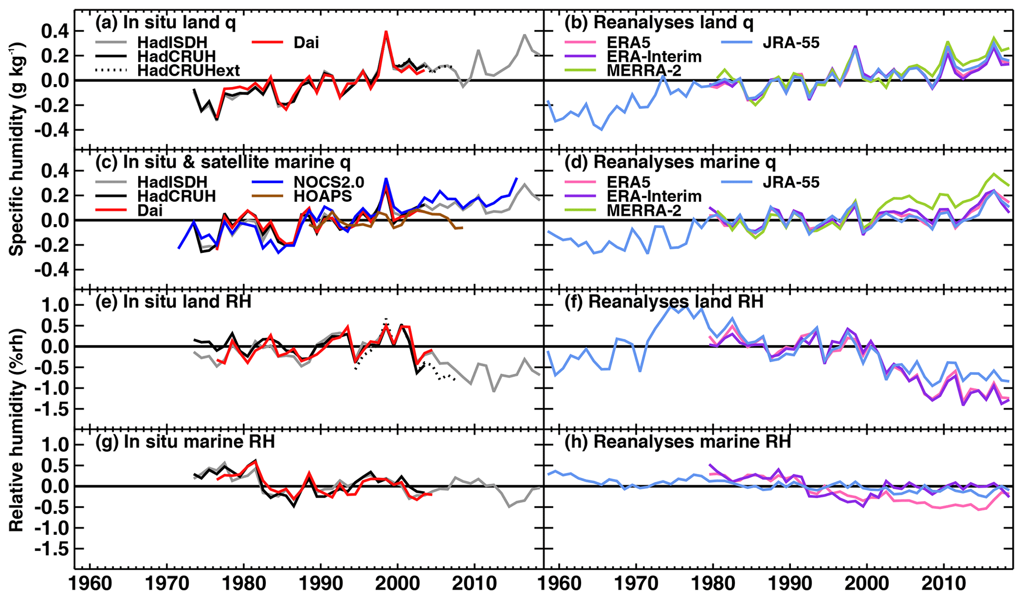
Figure 1 Global-average surface humidity annual anomalies (base period: 1979–2003). For in situ datasets, 2 m surface humidity is used over land and ∼10 m over the oceans. For the reanalysis, 2 m humidity is used across the globe. For ERA-Interim and ERA5, ocean-only points over open sea are selected, and background forecast values are used as opposed to analysis values to avoid incorporating biases from unadjusted ship data. All data have been given a mean of 0 over the common period 1979–2003 to allow direct comparison, with HOAPS given a mean of 0 over the 1988–2003 period. (Sources: HadISDH – Willett et al., 2013, 2014; HadCRUH – Willett et al., 2008; Dai – Dai, 2006; HadCRUHext – Simmons et al., 2010; NOCSv2.0 – Berry and Kent, 2009, 2011; HOAPS – Fennig et al., 2012; ERA-Interim – Dee et al., 2011; ERA5 – C3S, 2017; Hersbach et al., 2020; MERRA-2 – Gelaro et al., 2017; Bosilovich et al., 2015; JRA-55 – Kobayashi et al., 2015). Adapted from Willett et al. (2019).

A positive bias in global marine average relative humidity pre-1982 is apparent in Dai and HadCRUH and has previously been attributed to high frequencies of whole numbers in the dew point temperature observations prior to January 1982 (Willett et al., 2008). This is less clear in the global-average-specific-humidity time series. ICOADS (International Comprehensive Ocean-Atmosphere Data Set) documentation (http://icoads.noaa.gov/corrections.html, last access: June 2019) notes issues with the pre-1982 data, especially mixed-precision observations, where the air temperature has been recorded to decimal precision, but the dew point temperature is only available as a whole number. Such reporting was in accordance with the WMO ship code before 1982. The documentation notes a truncation error in the dew point depression, which would lead to a positive bias in relative humidity. Alternatively, Berry (2009) shows that patterns in the North Atlantic Oscillation coincide with this time period and could have played a role. The NOCSv2.0 product is based on reported wet-bulb temperature rather than dew point temperature, where decimal precision is usually present. Hence, the NOCSv2.0 product is expected to be unaffected by these rounding issues. Our analysis shows that changes to the code in January 1982 did not eliminate whole-number reporting, and high frequencies of whole numbers can be found throughout the record in both air temperature and dew point temperature (Sects. 2.4 and 3.4).

Clearly, there is a need for more and up-to-date in situ monitoring of humidity over ocean, especially for RH. The structural uncertainty in estimates can only be explored if there are multiple available estimates so a new product that explores different methodological choices and extends the record is complementary to the existing NOCSv2.0 product and reanalysis estimates. Here we report the development of a multivariable marine humidity analysis HadISDH.marine.1.0.0.2018f (Willett et al., 2020). HadISDH.marine is an integrated surface dataset of humidity led by the Met Office Hadley Centre, forming a companion product to the HadISDH.land monitoring product and enabling the production of a blended global land and ocean product. We use existing methods where possible from the systems used for building the long-running HadSST dataset (Kennedy et al., 2011a, b, 2019) and also use some of the bias adjustment methods employed for NOCSv2.0 (Berry and Kent, 2011). We have explored the data to design new humidity-specific processes where appropriate, particularly in terms of quality control and gridding.

HadISDH.marine is a climate-quality $\mathrm{5}{}^{\circ }\times \mathrm{5}{}^{\circ }$ gridded monthly mean product from 1973 to present (December 2018 at the time of writing) with annual updates envisaged. Fields are presented for surface (∼10 m) specific humidity, relative humidity, vapour pressure, dew point temperature, wet-bulb temperature, and dew point depression. Air temperature is also made available as a by-product, but less attention has been given to addressing temperature-specific biases. The product is intended for investigating long-term changes over large scales, and so efforts have been made to quality-control the data, ensure spatial and temporal homogeneity, adjust for known biases, and also estimate remaining uncertainty in the data. In particular, we estimate uncertainties from whole-number reporting and other measurement errors that have not been quantified before for marine humidity.

Section 2 discusses known issues with marine humidity data. Section 3 describes the source data and all processing steps. Section 4 presents the gridded product and explores the different methodological choices and comparison with NOCSv2.0 specific humidity and ERA-Interim marine humidity. This section also includes a first look at the blended land and marine HadISDH product for each variable. Section 5 covers data availability, and Sect. 6 concludes with a discussion of the strengths and weaknesses of the product.

2 Known issues affecting the marine humidity data

2.1 Daytime solar biases

Marine air temperature measurements on-board ships during the daytime are known to be affected by the heating of the ship or platform by the sun. This results in a positive bias during daylight and early night-time hours. The bias varies with sunlight strength or cloudiness (and thus also latitude), relative wind speed, and the size and material of the ship. This solar-heating bias affects both the wet-bulb and dry-bulb temperature measurements, but, as noted by Kent and Taylor (1996), the ships do not act as a source of humidity or change the humidity content of the air. As a result, biases in the specific humidity and dew point temperature due to the solar-heating errors will be negligible. However, care needs to be taken with relative humidity because estimates of the saturation vapour pressure from the uncorrected dry-bulb air temperature will be too high, leading to an underestimate in relative humidity. Ideally, relative humidity should be estimated using the corrected dry-bulb temperature to calculate the saturation vapour pressure and uncorrected wet- and dry-bulb temperature or dew point temperature to calculate the vapour pressure. Previously, efforts have been made to bias-adjust the air temperature observations for solar heating by modelling the extra heating over the superstructure of the ship, taking account of the relative wind speed, cloudiness, time of day, time of year, and latitude (Kent et al., 1993; Berry et al., 2004; Berry and Kent, 2011). These adjustments are complex, and so we have decided not to attempt to implement them for our first version of a marine humidity product given the wide variety of other issues we have accounted for. We have, however, produced daytime, night-time, and combined products to investigate differences that may be caused by the solar-heating bias. Later versions of HadISDH.marine that apply bias corrections for solar heating may reduce the number of daytime data removed.

2.2 Unaspirated-psychrometer bias

Humidity measurements can be made in a variety of ways. Instruments can be housed in a screen with ventilation slats, with or without additional artificial aspiration, or handheld in a sling or whirling psychrometer. There is information on instrument ventilation provided up to 2014. Approximately 30 % of ship observations have information in 1973, peaking at ∼75 % by the mid-1990s, as summarized in Fig. 2. Initially, slings were more common for the hygrometer and thermometer, but by 1982 a screen was more common. There is a tendency for the screened instruments, in the absence of artificial aspiration, to give a wet-bulb reading that is higher relative to the slings or whirling instruments where airflow is ensured by the whirling motion. Bias adjustments have been applied to unaspirated humidity observations by Berry and Kent (2011), building on previous bias adjustments of Josey et al. (1999) and Kent et al. (1993). They have also estimated the uncertainty in the bias adjustments. We implement a modified version of their method of bias adjustment for the unaspirated observation types (Sect. 3.3.1) and uncertainty estimation. Uncertainties from instrument bias adjustments will have some spatial and temporal correlation structure as the ships move around (Kennedy et al., 2011a).

2.3 Ship height inhomogeneity

Over time there has been a general trend for ship heights to increase. Kent et al. (2007, 2013) quantified the increase from an average of ∼16 m in 1973 to ∼24 m by the end of 2006. Instrument height information is available for some ships between the period of 1973 and 2014, providing heights for the barometer (HOB), thermometer (HOT), anemometer (HOA), and visual-observing platform (HOP). Figure 3 shows the availability of height information and the mean and standard deviation of heights per year in each category for the ship observations selected here. Similar to the ventilation metadata, height information availability is low in 1973, peaking mid-1990s to 2000 and then declining slightly. Prior to 1994 only the platform height was available from WMO Publication 47. This was replaced in 1994 by the barometer height and augmented with the thermometer and visual-observing heights from 2002 onwards (Kent et al., 2007). Anemometer heights have been available from WMO 47 since 1970. All four types of heights increase over time. We conclude that the mean height based on HOP, HOB, and HOT increases from 17 m in 1973 to 23 m by 2014, which differs slightly to that in Kent et al. (2007). If uncorrected, this likely leads to a small artificial decreasing trend in air temperature and specific humidity as, in general, these variables decrease with height away from the surface. The effect on relative humidity is less clear and depends on the relative effects on air temperature and specific humidity.

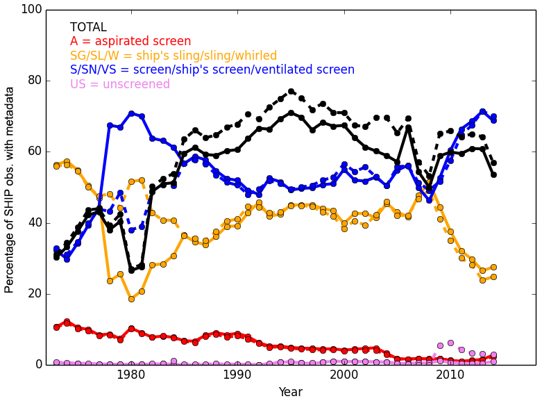
Figure 2 Availability of instrument exposure information (black) for ships (platform, PT $=\mathrm{0},\mathrm{1},\mathrm{2},\mathrm{3},\mathrm{4},\mathrm{5}$) for the hygrometer (hygrometer exposure, EOH; solid) and thermometer (thermometer exposure, EOT; dashed) for each year. All ICOADS 3.0.0 and 3.0.1 observations passing third-iteration quality control are included. The percentage of EOHs and EOTs in each exposure category is also shown. Aspirated (A) screens are shown in red. Handheld instruments (ship's sling, SG; sling, SL; whirling, W) are shown in orange. Unaspirated and unventilated screens (S) and ship's screens (SN) are shown in blue. Additionally, ventilated screens (VS) are also shown in blue as these are generally not artificially aspirated. Unscreened (US) observations are shown in violet.

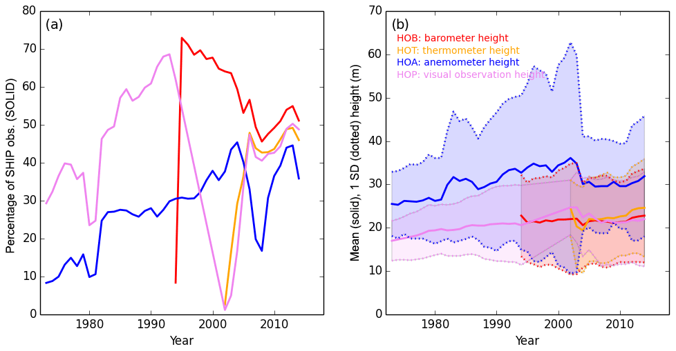
Figure 3 (a) Availability of instrument height information for ships (platform, PT $=\mathrm{0},\mathrm{1},\mathrm{2},\mathrm{3},\mathrm{4},\mathrm{5}$) for the barometer (HOB), thermometer (HOT), anemometer (HOA), and visual-observing platform (HOP) with (b) mean heights (solid lines) and standard deviations (dotted lines) for each year. All ICOADS 3.0.0 and 3.0.1 observations passing third-iteration quality control are included.

Prior studies (e.g. Berry and Kent, 2011; Berry 2009; Josey et al., 1999; Rayner et al., 2003; Kent et al., 2013) have applied height adjustments to the air temperature, specific humidity, and wind speed measurements to adjust the measurements to a common reference height and minimize the impact of the changing observing heights on the climate record. These have been based on boundary layer theory and the bulk formulae using the parameterizations of Smith (1980, 1988). In the absence of high-frequency observations of meteorological parameters for each observation location, allowing direct estimation of the surface fluxes, parameterizations have to be made, and an iterative approach is necessary to estimate a height adjustment (Sect. 3.3.2). We have followed these previous approaches and estimated height adjustments for all observations and variables of interest. Where observing heights are unavailable, we have made new estimates (Sect. 3.3.2). We have also provided an estimate of uncertainty on these height adjustments, which are larger where we have also estimated the height of the observation. The uncertainties from height adjustments will have some spatial and temporal correlation structure.

2.4 Whole-number reporting biases

Recording and reporting formats and practices have changed many times over the 20th century, affecting the climate record. Some formats required the wet-bulb temperature to be reported, others the dew point temperature, and some allowed either or both (https://www.wmo.int/pages/prog/amp/mmop/documents/publications-history/history/SHIP.html, last access: June 2019). Some earlier formats restricted space to reporting temperature to whole numbers only, and this practice has continued, with some ships continuing to report the dew point (or wet-bulb) temperature and sometimes even the dry bulb temperature to whole numbers. A practice of truncation of the dew point depression has been noted for the pre-1982 data (http://icoads.noaa.gov/corrections.html, last access: June 2019), which would result in spuriously high humidity (both in relative and actual terms). It is clear from the ICOADS3.0.0 and 3.0.1 data that there has been a practice of reporting values to whole numbers rather than decimal places, both for air temperature and dew point temperature. Rounding dew point temperature and air temperature could result in a ±0.5 ^∘C error individually or a just less than ±1 ^∘C error in dew point depression for a worst-case-scenario combination.

Whole-number reporting is an issue throughout the record for both variables; a breakdown of air and dew point temperature by decimal place over time is shown in Fig. S1 in the Supplement. Air temperature also shows a disproportionate frequency of half degrees (.5s). The percentage of whole numbers (.0s) declines over time, dramatically in the mid- to late 1990s for air temperature and from 2008 for both air and dew point temperature. This decline in the 1990s and in part also the general decline appear to be linked to an increase in numbers of moored buoys (see Fig. 5); a similar analysis without the moored buoys (not shown) shows greater consistency over time. The dew point temperature has two distinct peaks in whole-number frequency in the 1970s and mid-1990s to early 2010s. The latter peak is more pronounced when moored buoys are not included. The early peak is somewhat consistent with the restriction in transmission space prior to January 1982. This was previously thought to have been a possible cause of higher relative humidity over the period 1973–1981 compared to the rest of the record in the HadCRUH marine relative-humidity product (Willett et al., 2008). The pre-1982 moist bias was also apparent in the global marine relative-humidity product of Dai (2006), which like HadCRUH used dew point temperatures. The NOCSv2.0 product preferentially utilizes the wet-bulb temperatures from ICOADS, which are not affected by whole-number reporting to the same extent.

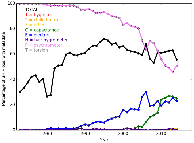
Figure 4 Availability of instrument type information (black) for ships (platform, PT $=\mathrm{0},\mathrm{1},\mathrm{2},\mathrm{3},\mathrm{4},\mathrm{5}$) for the hygrometer (TOH) for each year. All ICOADS 3.0.0 and 3.0.1 observations passing third-iteration quality control are included. The percentage of TOHs in each type category is also shown.

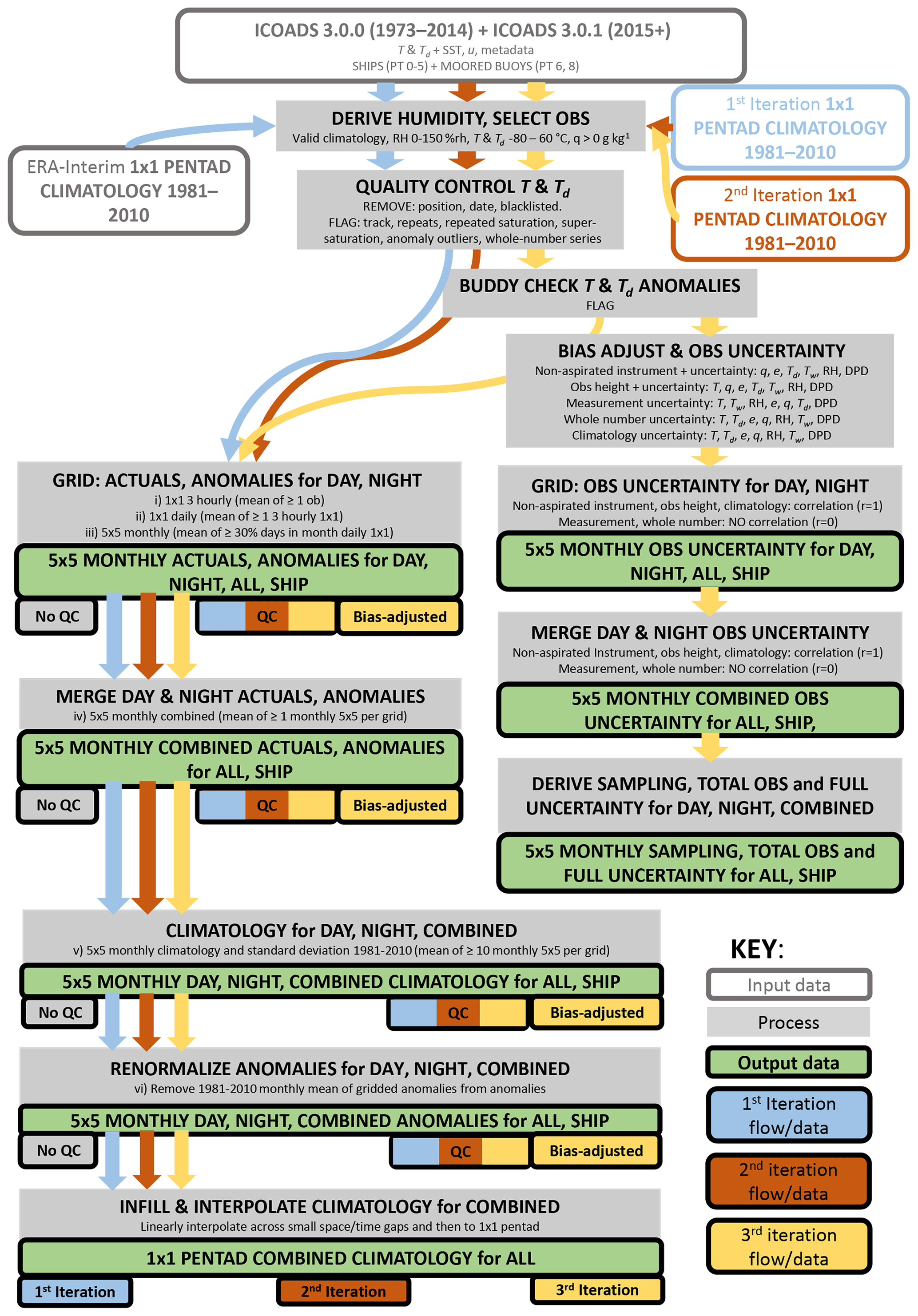
Figure 5 Flow chart of the build process from raw hourly observations to gridded fields. Note that the grey “no QC” output boxes are produced during the first iteration by selecting all data rather than those passing quality control.

Rounding of temperature alone should not affect the mean dew point temperature, specific humidity, or vapour pressure. However, as with the solar bias issue, it is sensitive to the point at which the reported dew point temperature was derived from the measured wet-bulb temperature or relative humidity. Most likely, this would be done prior to any rounding or truncating for reporting, but during later conversion of various sources into digital archives or corrections the dew point temperature may have been reconstructed (https://icoads.noaa.gov/e-doc/other/dupelim_1980, last access: June 2019). The effect of rounding on a monthly mean grid box average should be small as these errors are random and should reduce with averaging. However, there is a risk of removing very high humidity observations when a rounded dew point temperature then exceeds a non-rounded air temperature. Such values are removed by our supersaturation check (Sect. 3.2). We do not feel able to correct for this issue but instead include an uncertainty estimate for it. Overly frequent whole numbers are identified both during quality control track analysis and deck analysis. This is discussed in more detail in Sect. 3.4. Clearly, there are various issues that can arise linked to the precision of measured and reported data in addition to conversion between different units (e.g. Fahrenheit, Celsius, and kelvin; Fig. S1) and between different variables.

2.5 Measurement errors

All observations are subject to some level of measurement error, and, outside of precision laboratory experiments, the errors can be significant. The BIPM (International Bureau of Weights and Measures – Bureau International des Poids et Mesures) Guide to the Expression of Uncertainty in Measurement (BIPM, 2008) describes two categories of measurement uncertainty evaluation. A Type A evaluation estimates the uncertainty from repeated observations. A Type B evaluation of the uncertainty is based on prior knowledge of the instrument and observing conditions. Within this study we use a Type B evaluation, adjusting for systematic errors and inhomogeneities due to inadequate ventilation and changing observing heights (screen and height adjustments) and estimate the residual uncertainty. For the random components, we make the conservative assumption that all measurements were taken using a psychrometer (wet-bulb and dry-bulb thermometers), which allows us to follow the HadISDH.land methodology of Willett et al. (2013, 2014) as described in Sect. 3.4. An assessment of the frequency of hygrometer types (TOHs) within our selected ICOADS3.0.0 and 3.0.1 data shows this to be a fair assumption as the vast majority of ships (where metadata is available: ∼30 %, increasing to ∼70 % from 1973 to 1995 then decreasing to 60 % by 2014) are listed as being from a psychrometer (Fig. 4). Electric sensors are becoming more common and made up ∼30 % of observations by 2014 (the end of the metadata information). There are no instrument type metadata for ocean platforms or moored buoys. As it is likely that most buoy observations are made using RH sensors, we plan to develop an RH-sensor-specific measurement uncertainty in future versions.

2.6 Other sources of error

There are other issues specific to humidity measurements that may be further sources of error. Hygrometers that require a wetted wick (i.e. psychrometers) and thus a source of water are vulnerable to the wick drying out or contamination, especially by salt in the marine environment. The wick drying results in erroneous relative-humidity readings of 100 %rh, where the wet bulb essentially behaves identically to the dry-bulb thermometer. There can also be issues when the air temperature is close to freezing, depending on whether the wet bulb has become an ice bulb or not and whether wet-bulb or ice-bulb calculations are used in any conversions. Humidity observing in low temperatures can be generally problematic. For radiosondes, there has previously been a practice of recording a set low value when the humidity observation falls below a certain value (Wade, 1994; Elliott et al., 1998). It is debateable how likely such low humidity values are over oceans, and this practice has not been documented for ship observations. However, the set-value issue is something to look out for. Wet bulb thermometers (and other instruments) can experience some hysteresis at high humidity, where it takes some time to return to a lower reading. The wet bulb also requires adequate ventilation, which has been discussed above.

These can be accounted for to a large extent through quality control, but some error will inevitably remain. We can increase our confidence in the data by comparison with other available products and general expectation from theory.

3 Construction of the gridded dataset and uncertainty estimates

ICOADS Release 3.0 (Freeman et al., 2017) forms the base dataset for the HadISDH.marine humidity products. From January 1973 to December 2014 we use ICOADS.3.0.0 from http://rda.ucar.edu/datasets/ds540.0/ (last access: February 2019). These data include a unique identifier (UID) for each observation; a station identifier or ship call sign (ID); and metadata on instrument type, exposure, and height in many cases. From January 2015 onwards we use ICOADS.3.0.1 from the same source. These data include an ID and UID but no instrument metadata. It is likely that digitized metadata updates will be available periodically, depending on resource availability. Each observation is associated with a deck number. These are identifiers for ICOADS national and transnational subsets of data relating to source; for example deck 926 is the International Maritime Meteorological (IMM) data (https://icoads.noaa.gov/translation.html, last access: June 2019). We utilize the reported air temperature (T) and reported dew point temperature (T_d) as the source for our humidity products. Sea surface temperature (SST) and wind speed (u) are used for estimating height adjustments.

We calculate the specific humidity (q), relative humidity (RH), vapour pressure (e), wet-bulb temperature (T_w; not the thermodynamic wet bulb but a close approximation to it), and dew point depression (DPD) for each point observation. All humidity variables are derived from reported air and dew point temperature and ERA-Interim climatological (from the nearest $\mathrm{1}{}^{\circ }\times \mathrm{1}{}^{\circ }$ 5 d mean – pentad – grid box) surface pressure P_s using the set of equations from Willett et al. (2014), which can be found in Table S1 in the Supplement. This provides consistency with HadISDH.land for later merging. For consistency we use a fixed psychrometric coefficient that is identical for all observations when estimating the approximate thermodynamic wet-bulb temperature rather than the observed value, which depends on the type of psychrometer used. This is also consistent with what is done for HadISDH.land.

Additionally, we use ERA-Interim (Dee et al., 2011) reanalysis data to provide initial marine climatologies and climatological standard deviations for all variables to complete a first-iteration climatological outlier test. We extract $\mathrm{1}{}^{\circ }\times \mathrm{1}{}^{\circ }$ gridded 6-hourly 2 m air and dew point temperature and surface pressure to create 6-hourly humidity variables and then pentad climatologies and standard deviations over the 1981–2010 period. Note that three iterations are passed before finalizing the product. Only the first iteration uses ERA-Interim climatologies; later iterations use climatologies built from the previous iteration's quality-controlled observations (Sects. 3.2, 3.5, 4.1).

The construction process, including the three iterations and all outputs, is visualized in Fig. 5. Firstly, humidity variables are calculated. For the first iteration the hourly temperature and dew point temperature data are quality-controlled (Sect. 3.1) using an ERA-Interim-based climatology. The data are then gridded and merged, and a $\mathrm{1}{}^{\circ }\times \mathrm{1}{}^{\circ }$ pentad climatology is produced for each variable (Sect. 3.5). These first-iteration climatologies are then used to quality-control the original hourly data again; these data are then gridded and merged, and a second-iteration climatology is produced. The second-iteration climatology is then used to quality-control the original hourly data for a third and final time. It is during this third iteration that bias adjustments are applied and uncertainties estimated. The bias-adjusted data and uncertainties are then gridded and merged, and climatologies are created. For future annual updates the second-iteration climatologies will be used to apply quality control. Having three iterations enables incremental improvements to the climatology used to quality-control the data and therefore the skill of the quality control tests. It means that we can ensure that no artefacts remain from using ERA-Interim to quality-control the data initially. Arguably more iterations could be done, but each one is computationally expensive, and the difference between the second and third iteration is already very small.

3.1 Data selection

We screen all ICOADS data to sub-select only those observations passing the following criteria.

• There must be a non-missing T and T_d value.

• The platform type (PT) must be in one of the following categories: a ship (a US Navy or unknown vessel, a merchant ship or foreign military ship, an ocean station vessel off station or at an unknown location, an ocean station vessel on station, a lightship, an unspecified ship; PT = 0, 1, 2, 3, 4, 5) or a stationary buoy (moored or ice buoy; PT = 6, 8).

• The observation must have a climatology and standard deviation available for its closest $\mathrm{1}{}^{\circ }\times \mathrm{1}{}^{\circ }$ pentad.

• The observation must pass the gross error checks, calculated RH must be between 0 and 150 %rh (supersaturated values are flagged during quality control), both T and T_d must be between −80 and 65 ^∘C, and calculated q must be greater than 0.0 g kg⁻¹.

• Latitudes must be between −90 and 90^∘, and longitudes must be between −180 and 360^∘ (later converted to −180 to 180^∘).

• The hour, day, month, and year must be valid quantities.

• Any observation from Deck 732 from a specified year and region is blacklisted (Rayner et al., 2006; Kennedy et al., 2011a; Table S2).

Other marine products (e.g. NOCSv2.0; Berry and Kent, 2011) solely use ship observations due to the lack of buoy metadata available. We include moored buoys to produce climatologies because spatial coverage is of high importance. Our final version recommended to users is a ship-only (ship) product, but we have produced a combined (all) product for comparison. This will be reassessed for future versions. Figure 6a shows the number of observations included in the initial selection per year, broken down by platform type. The breakdown for daytime and night-time observations individually is near identical (not shown). Ship (PT =5) observations make up almost the entire dataset until the 1990s. After this the number of moored buoys grows significantly to make up around ∼50 % of observations from 2000 onwards. The ship-only product (removal of moored buoys) significantly reduces the number of observations in the recent period but gives a more consistent number of observations throughout the record. Our use of climate anomalies should mitigate biasing due to uneven sampling to some extent. Note that the number of grid boxes containing data may be a more relevant measure and that the vast increase in the number of buoys has not actually resulted in the same level of increase in spatial coverage in terms of grid boxes (compare 2018 annual average maps for ship-only and combined HadISDH.marine in Fig. S2).

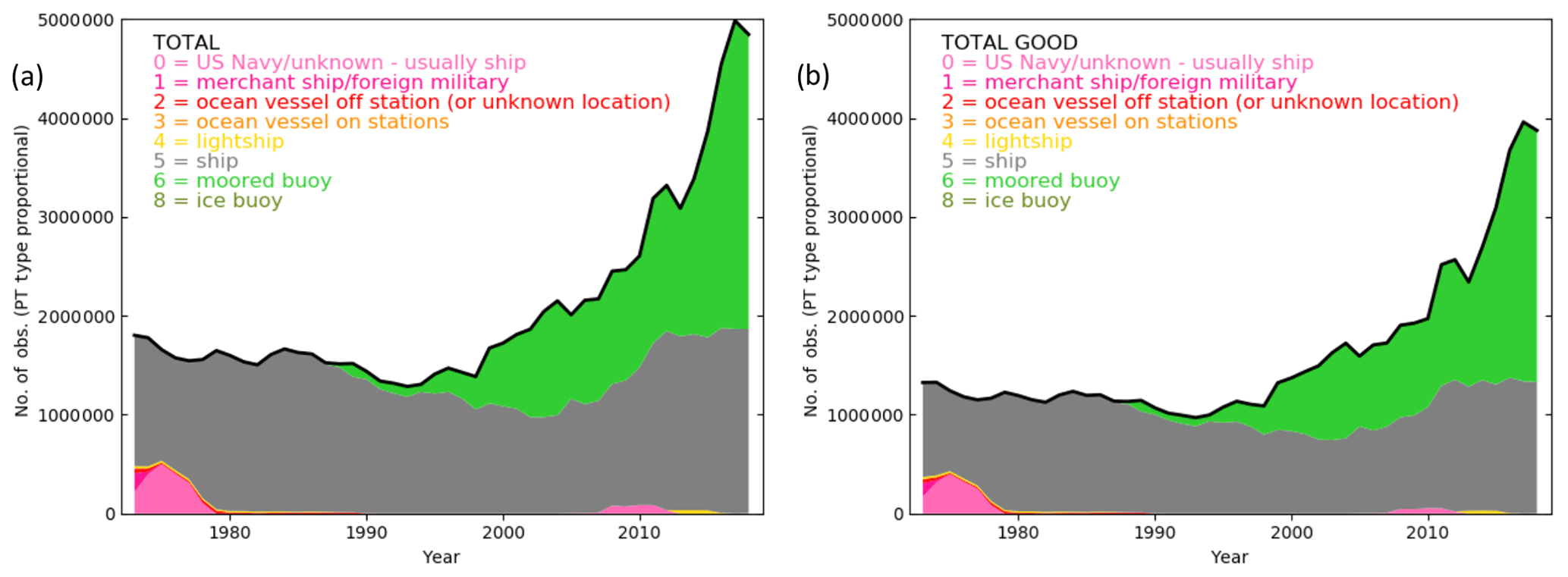
Figure 6 Annual observation count for the initial selection (a) and only those observations passing the final third-iteration quality control (b), broken down by platform type (PT).

3.2 Quality control processing

We have not used any of the preset flags from ICOADS processing to ensure methodological independence of HadISDH and a process that allows for exploration and analysis of different methodological choices. The quality control processing employed here largely follows the methodology for HadSST4 (Kennedy et al., 2019), with some changes to the climatology check and buddy check thresholds to increase regional sensitivity and additional humidity-specific checks. A flag for whole-number prevalence has also been added, but this is used for uncertainty estimation and not to remove an observation. All observations have their nearest $\mathrm{1}{}^{\circ }\times \mathrm{1}{}^{\circ }$ pentad mean climatology (source depends on iteration – Sect. 3.5) subtracted to create a climate anomaly.

Each observation is passed through a suite of quality control tests, which are summarized in Table 1 along with whether the quality control tests are used to remove or just to flag the observations and the stage of processing at which they are applied. The climatology check differs from the static HadSST3 threshold of climatology for air temperatures of ±8 ^∘C. We have allowed for a variable threshold depending on the nearest $\mathrm{1}{}^{\circ }\times \mathrm{1}{}^{\circ }$ pentad climatology standard deviation σ. This is set at 5.5σ. It accounts for the lower variability in the tropics and greater variability in the mid-latitudes. We have set minimum and maximum σ values of 1 and 4 ^∘C, respectively, resulting in a minimum range of ±5.5 ^∘C and a maximum range of ±22 ^∘C. Several thresholds were tested, with the selected threshold balancing avoiding acute cut-offs in the data distribution while still removing obviously bad data (Figs. S3 to S6). Given that outliers are assessed by comparing a point observation with a $\mathrm{1}{}^{\circ }\times \mathrm{1}{}^{\circ }$ pentad mean, the thresholds have to be relatively large.

Table 1 Description of quality control tests. n/a – not applicable

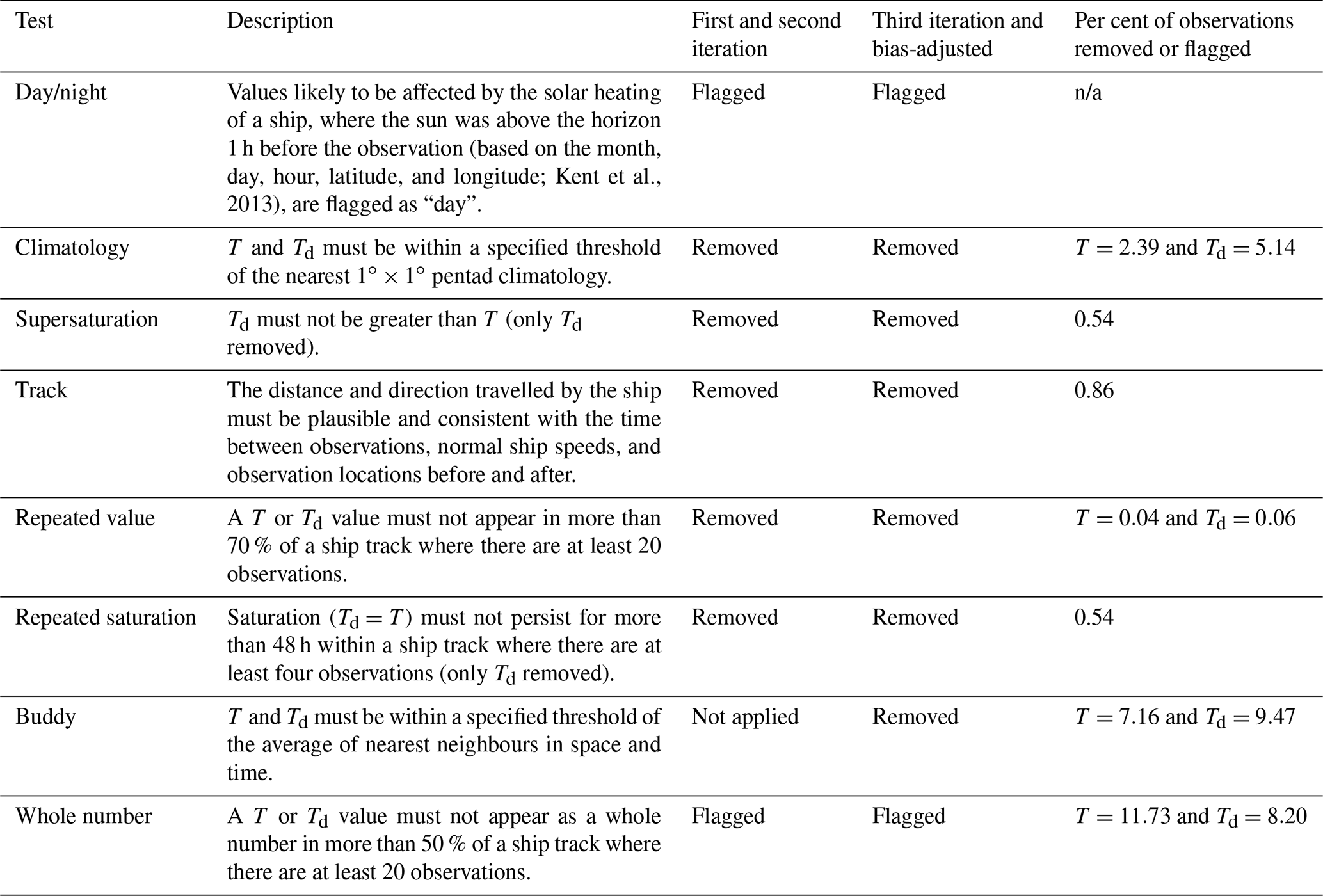
The buddy check compares each observation's climate anomaly with the average of the climate anomalies of its nearest neighbours in space and time, expanding the search area in space and time as necessary until at least one neighbour observation is found. The permitted difference is set by the climatological standard deviation of the candidate $\mathrm{1}{}^{\circ }\times \mathrm{1}{}^{\circ }$ pentad grid box multiplied by an amount dependent on the number of neighbours present. There are five levels of searches.

1. ±1^∘ latitude and longitude and ±2 pentads: the climatological standard deviation is multiplied by 5.5, 5.0, 4.5, and 4.0 for 1–5, 6–15, 16–100, and >100 neighbouring observations, respectively.

2. ±2^∘ latitude and longitude and ±2 pentads: the climatological standard deviation is multiplied by 5.5 for >1 neighbouring observation.

3. ±1^∘ latitude and longitude and ±4 pentads: the climatological standard deviation is multiplied by 5.5, 5.0, 4.5, and 4.0 for 1–5, 6–15, 16–100, and >100 neighbouring observations, respectively.

4. ±2^∘ latitude and longitude and ±4 pentads: the climatological standard deviation is multiplied by 5.5 for >1 neighbouring observation.

5. No neighbour ±2^∘ latitude and longitude and ±4 pentads: the threshold is set at 500.

The thresholds used for the buddy check are wider than those previously used in HadSST3. This is to account for the greater variability of air and dew point temperature and sparser observation coverage. It is only applied in the third iteration of the quality control (Sect. 3.5).

Figure 6 shows the final number of observations passing through initial selection and then third-iteration quality control by platform type (PT). The quality control does not significantly affect one platform over another. The performance of these tests is demonstrated for 4 example months in Figs. S3 to S6. These reveal a slight positive bias in the removed air temperature observations and negative bias in removed dew point temperature. Removals in terms of relative humidity and specific humidity similarly tend to have a negative bias. It is clear that the majority of grossly erroneous observations are removed. The change in climatology between iterations of the quality control process (Sect. 3.5) also makes a difference to removals. This is because the observation-driven climatologies do not provide complete spatial coverage and because the ERA-Interim climatologies are cooler and drier than the observations (Sect. 4.1). Removals are dense in the Northern Hemisphere and especially sparse around the tropics. The addition of the buddy check in the third iteration considerably increases the removal rate, noticeably over the Southern Hemisphere and the tropics.

The quality-control flagging rate for the third iteration reduces over time from ∼25 % to ∼18 %, as shown in Fig. S7. This is driven by the buddy check and track check. Proportionally more observations are flagged during the daytime than night-time, but the inter-annual behaviour is very similar. The daytime increase is driven by the larger number of air temperature buddy and climatology check failures. This could be due to the issue of solar heating of the ship structure during the daytime. The main source of test fails by a large margin is the buddy check, followed by the climatology check and track check. There does not appear to be a strong difference in the distribution of removals from each test between the 1973–1981 and 1982–1990 periods that might explain the pre-1982 moist bias (Fig. S8, Sect. 4.2). There is an increase in removals from repeated saturation and supersaturation events over time, particularly the late 2000s. This may be related to the decrease in psychrometer deployment over time and increase in electric and capacitance sensors as shown in Fig. 4. The latter have increased significantly since the mid-2000s.

The whole-number flags show very different behaviour to the other checks and to each other over time in Fig. S7. These depend on the ability to assign each observation to a track or voyage and the frequency of whole-number observations on that voyage; hence, these flags are not a true reflection of the whole-number frequency. Compared to the actual proportion of whole numbers shown in Fig. S1, these tend to exaggerate the annual patterns, but the shape is broadly similar. This method of identifying problematic whole numbers appears to under-sample the true distribution, especially for air temperature pre-1982. An additional deck-based check is applied later for estimating uncertainty from whole numbers (Sect. 3.4).

Note that the NOCSv2.0 dataset, with which we compare our specific-humidity data, includes an outlier check that removes data greater than 4.5 standard deviations from the climatological mean. This test has already been applied within the ICOADS format, and so the NOCSv2.0 excludes any data with ICOADS trimming flags set (Wolter, 1997). We do not use the trimming flags to select data. They also apply a track check based on Kent and Challenor (2006).

3.3 Bias adjustments and associated uncertainties

Given the issues raised in Sect. 2, it is desirable to attempt to adjust the observations to improve the spatial and temporal homogeneity and accuracy of the data. As discussed in Sect. 2.1, we have not attempted to adjust for solar biases in this first-version product. We have made adjustments for instrument and height biases and estimated uncertainties (summarized in Table 1) in these adjustments.

The availability of machine-readable metadata alongside each observation enables specific adjustment for known biases and inhomogeneities. This differs to the approach for the HadISDH.land dataset, where no substantial digitized metadata currently exist. By necessity, adjustment for biases (inhomogeneities) is done using the Pairwise Homogenization Algorithm (Menne and Williams, 2009). This is a neighbour-comparison-based statistical algorithm to detect change points and resolve the most reasonable adjustments. It is very likely that inhomogeneities that affect the land data such as instrument changes, instrument housing changes, and practice changes also affect the marine data. However, this level of detail is not available in the metadata nor is it straightforward to adjust for even if it were because of the mobile nature of ship data. Although a neighbour-based comparison is possible and useful at the single-observation level (e.g. buddy check), it is not useful in the manner in which it is used for land observations from static weather stations. Arguably, the region-wide biases such as increasing ship heights and ventilation biases are of greater concern for long-term trends than the more ship-specific inhomogeneity owing to instrument or housing changes. We acknowledge that, similar to the land data, there will be inhomogeneity or bias remaining within the HadISDH.marine dataset which we cannot detect or adjust for but argue that we have removed the large errors from the dataset. Future versions will take advantage of greater metadata and statistical tools as they become available.

3.3.1 Application of adjustments for biases from unaspirated instruments

We have shown that the majority of humidity observations have been made with a psychrometer (Fig. 4) and that 30 %–70 % of instruments with metadata available have been housed within a non-aspirated screen (Fig. 2). Berry and Kent (2011) found that applying a 3.4 % reduction to specific-humidity observations from non-aspirated screens was a reasonable adjustment to remove the bias relative to aspirated and well-ventilated observations (e.g. slings, whirled hygrometers, or artificially aspirated instruments). Some uncertainty remains after adjustment, which they estimated to be ∼0.2 g kg⁻¹. We have used the hygrometer exposure (EOH) metadata or the thermometer exposure (EOT) metadata if EOH does not exist. We assume good ventilation for any instruments that are aspirated (A), from a sling (SL) or ship's sling (SG), or from a whirling instrument (W). We assume poorer ventilation for instruments that are from a screen (S), ship's screen (SN), or are unscreened (US) and apply a bias adjustment. The reported exposure type of ventilated screens (VSs) does not appear to mean that the screen is artificially ventilated, and so bias adjustments are also applied to these. We do not apply adjustments to buoys and other non-ship data based on the assumption that these generally measure relative humidity directly. For any ship observations with no exposure information, we apply 55 % of the 3.4 % adjustment based on the mean percentage of observations with EOH metadata that require an adjustment over the 1973–2014 (metadata) period. This partial-adjustment factor follows the method of Berry and Kent (2011) and Josey et al. (1999) but differs in quantity. They assessed this over a shorter time period and found then that ∼30 % of observations were from poorly ventilated instruments.

To estimate the uncertainty in the non-aspirated-instrument adjustment U_i, we use the Berry and Kent (2011) and Josey et al. (1999) uncertainty estimate of 0.2 g kg⁻¹ and apply this in all cases where an adjustment or partial adjustment has been applied. This is treated as a standard uncertainty (1σ). In the case of partial adjustments for the ship observations with no metadata, there is large uncertainty in both the adjustment and adjusted value. To account for this we use the amount of what would have been a full 3.4 % adjustment in addition to the 0.2 g kg⁻¹ as the 1σ uncertainty.

To carry these adjustments and uncertainties to all other humidity variables, we start with q and then propagate the adjusted quantity and adjusted quantity plus uncertainty using the equations in Table S1. Using the original T (which does not need to be adjusted for poor ventilation) and ERA-Interim climatological surface pressure, e can be calculated from q. T_d and RH can be calculated from e and T. From these, the T_w and DPD can be calculated. The uncertainty is then obtained by subtracting the adjusted quantity from the adjusted quantity plus uncertainty for each variable.

3.3.2 Application of adjustments for biases from ship heights

After bias adjustment for poor ventilation, all variables are adjusted to approximately 10 m elevation. This serves to account for the inhomogeneity from the systematic increase in ship height over time and for spatial inhomogeneity between observations made at different heights. In the absence of height adjustments, increasing ship heights likely lead to a small decrease in air temperature and specific humidity over time (Berry and Kent, 2011) because these quantities generally decrease with height. As Fig. 3 shows, the standard deviations in ships' instrument heights exceed 5 m in most cases. Also, we have included buoys in the processing so far, and these can be very low (∼4 m; e.g. Gilhousen, 1987) relative to ship observing heights. The height of the hygrometer (HOH) must be estimated (HOHest) as no metadata are available. In the case of psychrometers, which are the most common instruments listed in the ship metadata, the wet- and dry-bulb thermometers are co-located. Figure 3 shows that the visual-observation height (HOP) is the most commonly available information, followed by the barometer height (HOB) and then thermometer height (HOT). It also shows the mean and standard deviation of all observing heights including the anemometer (HOA). Hence, HOHest is obtained using the following methods in order of preference.

1. HOP present and >2 m: HOHest μ= HOP, σ=1 m;

2. HOB present and >2 m: HOHest μ= HOB, σ=1 m

3. HOT present and >2 m: HOHest μ= HOT, σ=1 m;

4. HOA present and >12 m: HOHest μ= HOA −10, σ=9 m;

5. No height metadata: HOHest μ=16 m + the linear trend in mean HOP–HOB–HOT height to the date of observation, σ=4.6 m + the linear trend in standard deviation HOP–HOB–HOT height to the date of observation.

The μ and σ of the combined HOP, HOB, and HOT increases from 16 and 4.6 m, respectively, in January 1973 to 23 and 11 m, respectively, in December 2014. Kent et al. (2007) and Berry and Kent (2011) used 16 to 24 m between 1971 and 2007, so our estimate is very similar. The anemometer height is also required for the adjustments. We either use the provided HOA – as long as it is greater than 2 m – or set it to 10 m above the HOHest. All buoys are assumed to be observing at 4 m, with anemometers at 5 m (http://www.ndbc.noaa.gov/bht.shtml, last access: June 2019).

Once HOHest has been obtained for each observation, the air temperature and specific humidity are adjusted to 10 m using bulk flux formulae. The methodology, assumptions, and parameterizations largely follow those of Berry and Kent (2011), Berry (2009), Smith (1980, 1988), and Stull (1988). Essentially, the quantity of interest x can be adjusted to a reference height of 10 m as follows:

$$\begin{array}{}\text{(1)}& x_{\mathrm{10}}=x-{\displaystyle \frac{x_{\ast }}{\mathit{\kappa }}}\left(\ln \left({\displaystyle \frac{z_x}{\mathrm{10}}}\right)-{\mathit{\psi }}_x+{\mathit{\psi }}_{x\mathrm{10}}\right),\end{array}$$

where x_∗ is the scaling parameter specific to that variable (e.g. friction velocity in the case of u, characteristic temperature, or specific humidity in the case of T or q, respectively), κ is the von Karman constant (0.41 used here), z_x is the observation height of the variable of interest, ψ_x is the stability correction for the variable of interest and is a function of z_x∕L, ψ_x10 is the stability correction for the variable of interest at a reference height of 10 m and is a function of 10∕L, and L is the Monin–Obukov length.

An iterative approach (as done for Berry and Kent, 2011) is required to resolve Eq. (1) because we only have basic meteorological variables available at a single height for each observation. We start from T; q; u; sea surface temperature (SST); the co-located $\mathrm{1}{}^{\circ }\times \mathrm{1}{}^{\circ }$ grid box pentad climatological surface pressure from ERA-Interim (climP); HOHest, which becomes both z_q and z_t; and our estimated anemometer height, which becomes z_u. For some observations the SST or u is missing. If SST is missing it is given the same value as T, so in effect, no adjustment to T is applied. Either way, the SST is set to a minimum of −2 ^∘C and a maximum of 40 ^∘C. If u is <0.5 m s⁻¹ it is given a light wind speed of 0.5 m s⁻¹. If u is missing or >100 m s⁻¹ it is assumed to be erroneous but given a moderate wind speed of 6 m s⁻¹. We also approximate surface values T₀, q₀, and u₀, where T₀= SST, q₀=q_sat(SST)×0.98 and u₀=0. Clearly, with so many necessary approximations there are many different plausible methodological choices, hence the need for multiple independent analyses that explore these different choices in order to quantify the structural uncertainty.

We begin the iteration by assuming a value for L depending on assumed stability.

• If (SST – T) >0.2 ^∘C, then L is set to −50 m; unstable conditions are assumed.

• If (SST – T) $<-\mathrm{0.2}$ ^∘C, then L is set to 50 m; stable conditions are assumed.

• If (SST =T) ±0.2 ^∘C, then L is set to 5000 m; neutral conditions are assumed where L tends to ∞.

We also start with an assumption that the 10 m wind speed in neutral conditions u_10n=u. The iteration is continued until L converges to within 0.1 m, which it generally does. If after 100 iterations there is no convergence, we either apply no adjustment or, if absolute L is large (>500 m), we assume neutral conditions and take L (and all other parameters) as they are. In cases where u_∗ is very large (it should be <0.5 m s⁻¹; Stull, 1988), we also apply no adjustment. The iteration involves 21 steps as described in the Supplement.

For most observations we arrive at a plausible L, friction velocity u_∗, ψ_x, and ψ_x10. We then calculate the scaling parameters T_∗ and q_∗:

$$\begin{array}{}\text{(2a)}& {\displaystyle }& {\displaystyle }{T}_{\ast }=\mathit{\kappa }{\left(\ln \left({\displaystyle \frac{z_t}{z_{t\mathrm{0}}}}\right)-{\mathit{\psi }}_t\right)}^{-\mathrm{1}}\left(T-T_{\mathrm{0}}\right)\text{(2b)}& {\displaystyle }& {\displaystyle }{q}_{\ast }=\mathit{\kappa }{\left(\ln \left({\displaystyle \frac{z_q}{z_{q\mathrm{0}}}}\right)-{\mathit{\psi }}_q\right)}^{-\mathrm{1}}\left(q-q_{\mathrm{0}}\right),\end{array}$$

where the neutral stability heat transfer coefficient z_t0=0.001 m and the neutral stability moisture transfer coefficient z_q0=0.0012 m (Smith, 1988). The adjusted values for T₁₀ and q₁₀ can then be calculated from Eq. (1). From these we recalculate the other humidity variables using the equations in Table S1.

There is uncertainty in the obtained HOHest. Given that this is a best estimate, we assume that the uncertainty in the height is normally distributed and use the standard deviation in the height estimate HOHest to calculate an uncertainty range in the height-adjusted value x (where x is any of T, q, etc.) of xH_min to xH_max. Following the “two out of three chances” rule in the BIPM Guide to the Expression of Uncertainty in Measurement (BIPM, 2008), the standard uncertainty (1σ) for the height-adjusted value (U_h) is then given by

$$\begin{array}{}\text{(3)}& U_{\mathrm{h}}={\displaystyle \frac{x{H}_{max}-x{H}_{min}}{\mathrm{2}}}.\end{array}$$

The range xH_min to xH_max depends on the source of HOHest and associated σ, as listed above. There are several scenarios where estimating the uncertainty in this way is not possible, or calculation of an adjustment is not possible. Also, U_h for buoys is highly uncertain given the lack of height information available. These alternative scenarios are documented in Table 2.

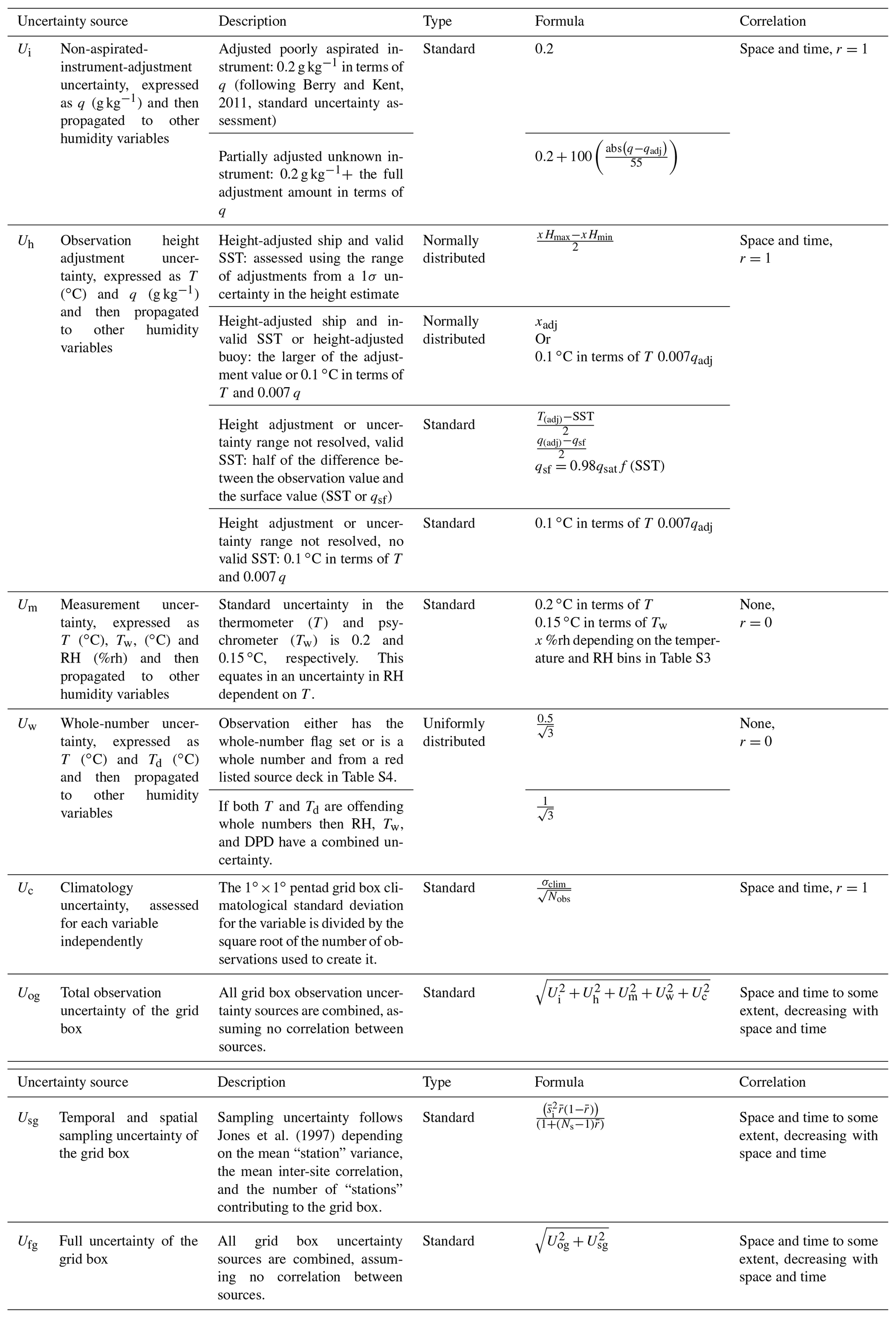
Table 2 Description of the uncertainty elements affecting marine humidity. All uncertainties are assessed as 1σ uncertainty.

3.4 Estimating residual uncertainty at the observation level

Three other sources of uncertainty affect the marine humidity data at the observation level. These are measurement uncertainty U_m, climatology uncertainty U_c, and whole-number uncertainty U_w. These are all assessed as 1σ standard uncertainties.

We have estimated U_m for each observation following the method used for HadISDH.land (Willett et al., 2013, 2014). This assumes that humidity was measured using a psychrometer, which is a reasonable assumption for the marine ship data (Fig. 4). The HadISDH.land measurement uncertainty is based on an estimated standard (1σ) uncertainty in the wet-bulb and dry-bulb instruments of 0.15 and 0.2 ^∘C, respectively. As shown in Table S3, the equivalent uncertainty for the other variables depends on the temperature. The uncertainty is applied as a standard uncertainty in RH depending on which bin the air temperature falls in. This is then propagated through the other variables starting with vapour pressure using the equations in Table S1.

Whole numbers of air and/or dew point temperature that have been flagged as such during quality control (Sect. 3.2) or that belong to a source deck or year where whole numbers make up more than 2 times the frequency of other decimal places (Table S4) are given an uncertainty U_w. These decks and years where whole numbers are very common differ for air and/or dew point temperature. Clearly with so many decks affected, the removal of entire decks to remove any whole-number biasing could easily reduce sampling to critically low levels. We cannot distinguish between observations that have been rounded versus those that have been truncated, so we assume that all offending whole numbers have been rounded. This means that the value could be anywhere within ±0.5 ^∘C, with a uniform distribution. Hence, where only air or dew point temperature is an offending whole number, the standard 1σ uncertainty expressed in air or dew point temperature (^∘C) is

$$\begin{array}{}\text{(4)}& U_{\mathrm{w}}={\displaystyle \frac{\mathrm{0.5}}{\sqrt{\mathrm{3}}}}.\end{array}$$

Where both air and dew point temperature are offending whole numbers, the standard 1σ uncertainty expressed in air or dew point temperature (^∘C) for dew point depression, relative humidity, and wet-bulb temperature is

$$\begin{array}{}\text{(5)}& U_{\mathrm{w}}={\displaystyle \frac{\mathrm{1}}{\sqrt{\mathrm{3}}}}.\end{array}$$

There is uncertainty U_c in the climatological values used to calculate climate anomalies because of missing data over time, uneven and sparse sampling in space, and also the inevitable mismatch between a point observation and a $\mathrm{1}{}^{\circ }\times \mathrm{1}{}^{\circ }$ gridded pentad climatology. This uncertainty reduces with the number of observations contributing to the climatology N_obs and with the variability of the region σ_clim. The climatologies used to create the anomalies have undergone spatial and temporal interpolation to move from $\mathrm{5}{}^{\circ }\times \mathrm{5}{}^{\circ }$ gridded monthly climatologies and climatological standard deviations σ_clim to maximize coverage, and so it is not straightforward to assess the number of observations contributing to each $\mathrm{1}{}^{\circ }\times \mathrm{1}{}^{\circ }$ gridded pentad climatology, and the true σ_clim is likely greater. The minimum number of years required to be present over the 30-year climatology period is 10. Therefore, we assume a worst-case scenario of N_obs=10. Hence, for a standard 1σ uncertainty the following equation applies:

$$\begin{array}{}\text{(6)}& U_{\mathrm{c}}={\displaystyle \frac{{\mathit{\sigma }}_{\mathrm{clim}}}{\sqrt{N_{\mathrm{obs}}}}}.\end{array}$$

3.5 Gridding of actual and anomaly values and uncertainty

To create a quasi-global monitoring product, the raw observations need to be gridded. The spatial density is too low for high-resolution grids, and the intended purpose is for this marine product to be blended with the HadISDH.land humidity product, which is on a $\mathrm{5}{}^{\circ }\times \mathrm{5}{}^{\circ }$ grid at monthly resolution. Hence, the point hourly observations must be averaged to monthly mean gridded values.

The sparsity of the data means that there is a risk of bias due to poor sampling. A $\mathrm{5}{}^{\circ }\times \mathrm{5}{}^{\circ }$ grid box covers an area greater than 500 km²×500 km², which, despite the large correlation decay distances of both temperature and humidity, can include considerable variability. Furthermore, a monthly mean can be made up of a strong diurnal cycle and considerable synoptic variability. This is minimized by the use of climate anomalies, but regardless, care should be taken to ensure sufficient sampling density while maximizing coverage where possible.

Several data-density criteria were trialled to balance spatial coverage and poor representativeness (high variance) of the grid box averages. Climate anomalies are created at the raw observation level by subtracting the nearest $\mathrm{1}{}^{\circ }\times \mathrm{1}{}^{\circ }$ pentad climatology (1981–2010), and so we can grid both the actual values and the anomalies. Gridding of the anomalies is safer than gridding actual values in terms of biasing through poor sampling density because the correlation length scales of anomalies are higher than for actual temperatures. Initially, ERA-Interim is used to provide a climatology. This then requires an iterative approach to produce an initial observation-based climatology and improve the climatology through quality control. To reduce biasing further we grid the data in six stages to create an average at each stage. The entire process including quality control, bias adjustment, gridding, and three iterations is shown diagrammatically in Fig. 5 and each gridding stage described below.

1. Create $\mathrm{1}{}^{\circ }\times \mathrm{1}{}^{\circ }$ 3-hourly gridded means of the hourly observations of actuals and anomalies; there must be at least one observation.

2. Create separate $\mathrm{1}{}^{\circ }\times \mathrm{1}{}^{\circ }$ daytime and night-time gridded means of the $\mathrm{1}{}^{\circ }\times \mathrm{1}{}^{\circ }$ 3-hourly gridded mean actuals and anomalies; there must be at least one $\mathrm{1}{}^{\circ }\times \mathrm{1}{}^{\circ }$ 3-hourly grid.

3. Create $\mathrm{5}{}^{\circ }\times \mathrm{5}{}^{\circ }$ monthly daytime and night-time gridded means of the $\mathrm{1}{}^{\circ }\times \mathrm{1}{}^{\circ }$ daytime and night-time gridded mean actuals and anomalies; there must be at least 0.3× days in the month of $\mathrm{1}{}^{\circ }\times \mathrm{1}{}^{\circ }$ daily grids.

4. Create combined $\mathrm{5}{}^{\circ }\times \mathrm{5}{}^{\circ }$ monthly gridded means of the $\mathrm{5}{}^{\circ }\times \mathrm{5}{}^{\circ }$ monthly daytime and night-time gridded mean actuals and anomalies; there must be at least one $\mathrm{5}{}^{\circ }\times \mathrm{5}{}^{\circ }$ monthly daytime or night-time gridded mean.

5. Create 1981–2010 $\mathrm{5}{}^{\circ }\times \mathrm{5}{}^{\circ }$ monthly mean climatologies and standard deviations from the $\mathrm{5}{}^{\circ }\times \mathrm{5}{}^{\circ }$ monthly gridded means of actuals and anomalies; there must be at least 10 $\mathrm{5}{}^{\circ }\times \mathrm{5}{}^{\circ }$ monthly gridded means.

6. Renormalize the gridded anomalies by subtracting the monthly anomaly 1981–2010 climatology to remove biases from use of the previous climatology iteration (Sect. 4.1).

At each iteration the gridded observation-based climatologies are infilled linearly over small gaps in space and time and then interpolated down to $\mathrm{1}{}^{\circ }\times \mathrm{1}{}^{\circ }$ pentad resolution. The observations are too sparse to create such high-resolution grids directly.

The observation uncertainties also need to be gridded and the total observation uncertainty U_o calculated. Ships move around, and so their uncertainties also track around the globe. This means that the uncertainty in any one point or grid box bears some relationship to nearby points or grid boxes over time and space and cannot be treated independently. Correlation needs to be accounted for in both gridding and subsequently creating regional averages from grid boxes to avoid underestimation. The five sources of observation uncertainty are summarized in Table 2. The non-aspirated-instrument-adjustment uncertainty U_i, height adjustment uncertainty U_h, and climatology uncertainty U_c persist over time and space as ships move around. These are accordingly treated as correlating completely within 1 grid box month. The measurement uncertainty U_m and whole-number uncertainty U_w are likely to differ from observation to observation, and so they are treated as having no correlation within 1 grid box month. Hence, observation uncertainty sources are first gridded individually, following the first four steps outlined above and taking into account correlation where necessary. For those that do not correlate (U_m and U_w), the grid box mean uncertainties U_gb for each source are combined over N points in time and space as follows:

$$\begin{array}{}\text{(7)}& U_{\mathrm{gb}}={\displaystyle \frac{\sqrt{a^{\mathrm{2}}+b^{\mathrm{2}}\mathrm{\dots }+n^{\mathrm{2}}}}{N}}.\end{array}$$

For those sources that do correlate (U_c, U_i, and U_h), assuming r=1, the grid box mean uncertainties U_gb for each source are combined over N points in time and space as follows:

$$\begin{array}{}\text{(8)}& U_{\mathrm{gb}}={\displaystyle \frac{a+b\mathrm{\dots }+n}{N}}.\end{array}$$

To create the total observational uncertainty for each grid box, the grid box quantities of the five uncertainty sources can then be combined in quadrature:

$$\begin{array}{}\text{(9)}& U_{\mathrm{o}}=\sqrt{U_{\mathrm{c}}^{\mathrm{2}}+U_{\mathrm{m}}^{\mathrm{2}}+U_{\mathrm{w}}^{\mathrm{2}}+U_{\mathrm{h}}^{\mathrm{2}}+U_{\mathrm{i}}^{\mathrm{2}}}.\end{array}$$

Given the general sparsity of observations across each grid box month and the uneven distribution of observations across each grid box and over time, there is also a grid box sampling uncertainty component, U_s. This is estimated directly at the $\mathrm{5}{}^{\circ }\times \mathrm{5}{}^{\circ }$ monthly grid box level and follows the methodology applied for HadISDH.land (Willett et al., 2013, 2014), denoted SE², which is based on station-based observations from Jones et al. (1997):

$$\begin{array}{}\text{(10)}& U_{\mathrm{s}}={\displaystyle \frac{\left({\overline{s}}_{\mathrm{i}}^{\mathrm{2}}\overline{r}\left(\mathrm{1}-\overline{r}\right)\right)}{\left(\mathrm{1}+\left(N_{\mathrm{s}}-\mathrm{1}\right)\overline{r}\right)}},\end{array}$$

where ${\overline{s}}_{\mathrm{i}}^{\mathrm{2}}$ is the mean variance of individual stations within a grid box, $\overline{r}$ is the mean inter-site correlation, and N_s is the number of stations contributing to the grid box mean in each month. The mean variance of individual stations within the grid box is estimated as

$$\begin{array}{}\text{(11)}& {\overline{s}}_{\mathrm{i}}^{\mathrm{2}}={\displaystyle \frac{\left({\widehat{S}}^{\mathrm{2}}{N}_{\mathrm{SC}}\right)}{\left(\mathrm{1}+\left(N_{\mathrm{SC}}-\mathrm{1}\right)\overline{r}\right)}},\end{array}$$

where ${\widehat{S}}^{\mathrm{2}}$ is the variance of the grid box monthly anomalies over the 1982–2010 climatology period, and N_SC is the mean number of stations contributing to the grid box over the climatology period. The mean inter-site correlation is estimated by

$$\begin{array}{}\text{(12)}& \overline{r}={\displaystyle \frac{x_{\mathrm{0}}}{X}}\left(\mathrm{1}-\exp \left(-{\displaystyle \frac{x_{\mathrm{0}}}{X}}\right)\right),\end{array}$$

where X is the diagonal distance across the grid box, and x₀ is the correlation decay length between grid box means. We calculate x₀ as the distance (grid box midpoint to midpoint) at which correlation reduces to 1∕e. To account for the fact that marine observations generally move around at each time point, we use the concept of pseudo-stations to modify this methodology. For any one day there could be 25 $\mathrm{1}{}^{\circ }\times \mathrm{1}{}^{\circ }$ grid boxes, and so we assume that the maximum number of pseudo-stations per grid box is 25, which is broadly consistent with the number of stations per grid box in HadISDH.land. Over a month then, there could be a maximum of 775 $\mathrm{1}{}^{\circ }\times \mathrm{1}{}^{\circ }$ daily grid boxes contributing to each $\mathrm{5}{}^{\circ }\times \mathrm{5}{}^{\circ }$ monthly grid box. Given ubiquitous missing data and sparse sampling, the maximum in practice is closer to 600. Using these values we then scale the actual number of $\mathrm{1}{}^{\circ }\times \mathrm{1}{}^{\circ }$ daily grid boxes contributing to each $\mathrm{5}{}^{\circ }\times \mathrm{5}{}^{\circ }$ monthly grid box to provide a pseudo-station number between 1 and 25 for each month (N_s) and then the average over the climatology period (N_SC).

The grid box U_o and U_s uncertainties are then combined in quadrature, assuming no correlation between the two sources. This gives the full grid box uncertainty U_f. Calculation of regional-average uncertainty and spatial coverage uncertainty is covered in Sect. 4.

4 Analysis and validity of the gridded product

The final gridded marine humidity monitoring product presented as HadISDH.marine.1.0.0.2018f is the result of the third-iteration quality control and bias adjustment of ship-only observations average into $\mathrm{5}{}^{\circ }\times \mathrm{5}{}^{\circ }$ gridded monthly means (Fig. 5). There are four reasons for only using the ship observations. Firstly, the increase in spatial coverage in the combined ship–buoy product is actually fairly small (Fig. S2) and only during the latter part of the record. Secondly, a dataset intended for detecting long-term changes in climate should have reasonably consistent input data and coverage over time. Thirdly, we believe that the buoy data are less reliable given their proximity to the sea surface and exposure to sea spray contamination in addition to the lower maintenance frequency compared to ship data. Fourthly, there are no metadata available for buoy observations, which makes it difficult to apply necessary bias adjustments or estimate uncertainties. Actual monthly means, anomalies from the 1981–2010 climatology (not standardized by division with the standard deviation), the climatological means and standard deviation of the climatologies, uncertainty components, and number of observations for both products are all made available as netCDF from https://www.metoffice.gov.uk/hadobs/hadisdh/ (last access: June 2019).

4.1 Comparison of climatologies between HadISDH.marine and ERA-Interim

At the end of each iteration (Fig. 5), observation-based climatology fields are created at both the monthly $\mathrm{5}{}^{\circ }\times \mathrm{5}{}^{\circ }$ grid and, by interpolation, pentad $\mathrm{1}{}^{\circ }\times \mathrm{1}{}^{\circ }$ grid (Sect. 3.5). These are then used to quality-control and create anomaly values for the next iteration. Hence, the second-iteration quality-controlled data are used to build the final third iteration, and therefore there should be no lasting effect from having used the ERA-Interim fields initially. The quality-controlled, buddy-checked, and bias-adjusted third iteration is used to create the final climatology provided to users.

To compare the use of ERA-Interim versus the observation-based climatology to calculate anomalies and quality-control the data, we show difference maps of the second iteration minus ERA-Interim pentad $\mathrm{1}{}^{\circ }\times \mathrm{1}{}^{\circ }$ grid climatologies and climatological standard deviations in Figs. S9 to S14 for a selection of pentads and variables. Note that ERA-Interim fields are for 2 m above the ocean surface, whereas the raw observations range between approximately 10 and 30 m above the surface. In normal conditions we may therefore expect ERA-Interim to provide climatologies that are warmer and moister than the observations. However, overall, ERA-Interim appears drier (both in absolute and relative terms) and cooler than the observation-based climatologies. For humidity this is consistent with the results of Kent et al. (2014). For the majority of grid boxes these differences are within ±2 g kg ⁻¹, ±2 %rh, and ±2^∘C. However, differences are especially strong around coastlines, with magnitudes exceeding ±10 g kg ⁻¹, ±10 %rh, and ±10^∘C. This is to be expected given that ERA-Interim coastal grid boxes will include effects from land, especially at the relatively coarse $\mathrm{1}{}^{\circ }\times \mathrm{1}{}^{\circ }$ grid resolution. For relative humidity there are more regions where ERA-Interim is more saturated, and there is more seasonality in the differences. Relative humidity is less stable spatially and on synoptic timescales and also more susceptible to biases and errors than specific humidity and air temperature, largely because it is affected by errors in both air temperature and dew point temperature. For temperature, the coastal difference can be positive or negative depending on the season.

The climatological standard deviations are generally lower in the second-iteration observations compared to ERA-Interim. Differences are generally between ±2 g kg ⁻¹, %rh, and ^∘C, but for relative humidity there are expansive regions in the extratropics to mid-latitudes, especially in the Northern Hemisphere, where climatological standard deviations are up to 5 %rh lower in the observations. The generally lower variability in the observation-based climatology is to be expected given the interpolation from monthly mean resolution and interpolation over neighbouring grid boxes where data coverage is limited. However, much of the tropics, particularly in the Southern Hemisphere, tend to show more variability in the observations. Similarly, many of the peripheral grid boxes (those at the edge of the spatial coverage and therefore more likely to be interpolated from nearby grid boxes rather than based on actual data) show higher variability for specific and relative humidity and lower variability for air temperature. All of these grid boxes are in data-sparse regions, which likely contributes to the higher variability. Ideally, observation-based climatologies would be created directly at the pentad $\mathrm{1}{}^{\circ }\times \mathrm{1}{}^{\circ }$ grid, but this severely reduces spatial coverage of the climatology fields and any product based on them. A balance has to be made between coverage and quality.

Annual mean $\mathrm{5}{}^{\circ }\times \mathrm{5}{}^{\circ }$ climatologies (no interpolation) from the third-iteration quality-controlled, bias-adjusted ship-only product are shown in Fig. 7 for specific humidity, relative humidity, air temperature, and dew point temperature. These have a minimum data presence threshold of 10 years for each month over the climatology period and at least 9 climatological months present for the annual climatology. Data coverage is virtually non-existent in the Southern Hemisphere below 40^∘ S, and Northern Hemisphere coverage diminishes drastically above 60^∘ N. These climatologies are as expected for these variables and compare well in terms of broad spatial patterns with ERA-Interim (not shown). There is good spatial consistency considering that no interpolation has been conducted, meaning that any erroneous grid boxes should stand out. We conclude that, as a first-version product, these climatologies look reasonable.

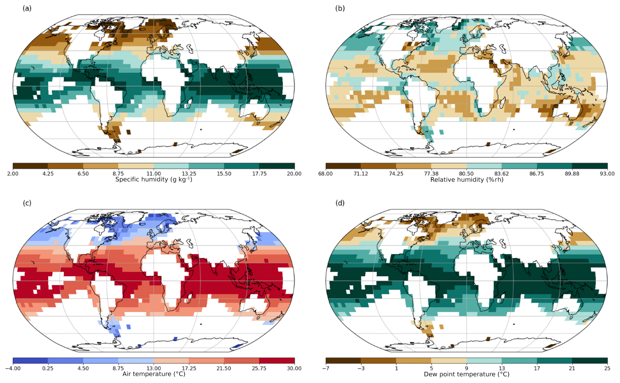
Figure 7 Annual mean climatologies relative to 1981–2010 for (a) specific humidity (g kg⁻¹), (b) relative humidity (%rh), (c) air temperature (^∘C), and (d) dew point temperature (^∘C) for third-iteration quality-controlled and bias-adjusted ship version. Climatological means are calculated for grid boxes and months with at least 10 years present over the climatology period. Annual mean climatologies require at least 9 months of the year to be represented climatologically.

4.2 Analyses of global averages for various processing stages and with other products

Global-average quantities are key measures of climate change, and so we focus here on the differences arising from the various processing steps of HadISDH.marine along with the NOCSv2.0 specific humidity and ERA-Interim reanalysis products. Global averages have been created by weighting each grid box by the cosine of its latitude at the grid box centre. All time series shown are the renormalized anomalies with a mean of 0 over the 1981–2010 period. Figures 8 to 11 show time series for specific humidity, relative humidity, dew point temperature, and air temperature, respectively. Decadal linear trends (shown) are computed using ordinary least-squares regression with ranges representing the 90th-percentile confidence interval calculated using AR(1) correction (Santer et al., 2008).

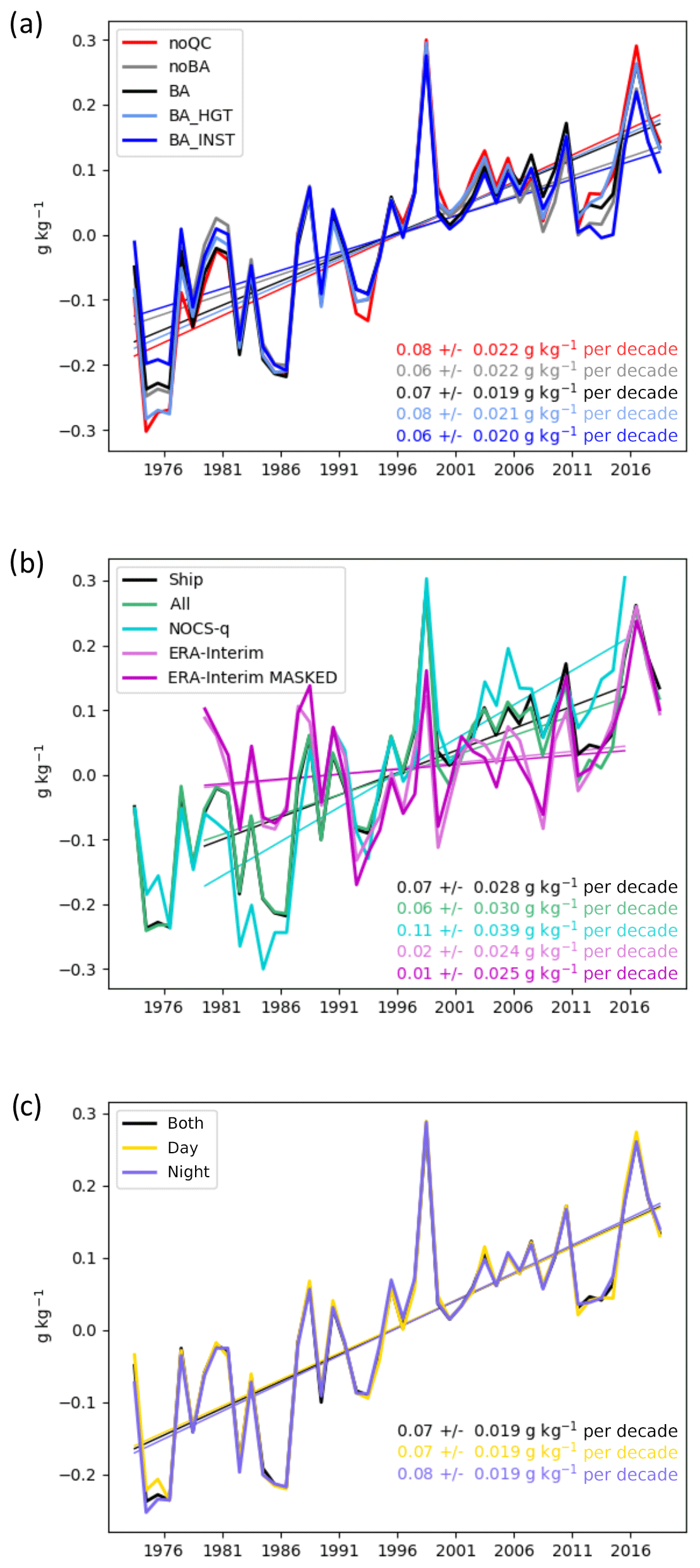
Figure 8 Global annual average anomaly time series and decadal trends (±90 % confidence interval) for specific humidity. (a) Processing comparison for ships only: raw data (noQC), third-iteration quality-controlled with no bias adjustment (noBA), third-iteration quality-controlled and bias-adjusted (BA), third-iteration quality-controlled and bias-adjusted for ship height only (BA_HGT), third-iteration quality-controlled and bias-adjusted for instrument ventilation only (BA_INST). (b) Platform and alternative product comparison: third-iteration quality-controlled and bias-adjusted for ships only (ship), third-iteration quality-controlled and bias-adjusted for ships and moored buoys (all), NOCSv2.0 in situ quality-controlled and bias-adjusted product based on ships only (NOCS-q), ERA-Interim reanalysis 2 m fields using complete ocean coverage at the $\mathrm{1}{}^{\circ }\times \mathrm{1}{}^{\circ }$ scale (ERA-Interim), ERA-Interim reanalysis 2 m fields using complete ocean coverage at the $\mathrm{1}{}^{\circ }\times \mathrm{1}{}^{\circ }$ scale and masked to HadISDH.marine spatio-temporal coverage (ERA-Interim MASKED). Trends cover the common 1979–2015 period. The 1979–2018 trends for ERA-Interim are 0.03±0.028 and 0.03±0.027 for the full and masked versions, respectively. (c) Time of observation comparison for third-iteration quality-controlled and bias-adjusted for ships only: all times (both), daytime hours only (day), night-time hours only (night). Linear trends were fitted using ordinary least-squares regression with AR(1) correction applied when calculating confidence intervals (Santer et al., 2008).

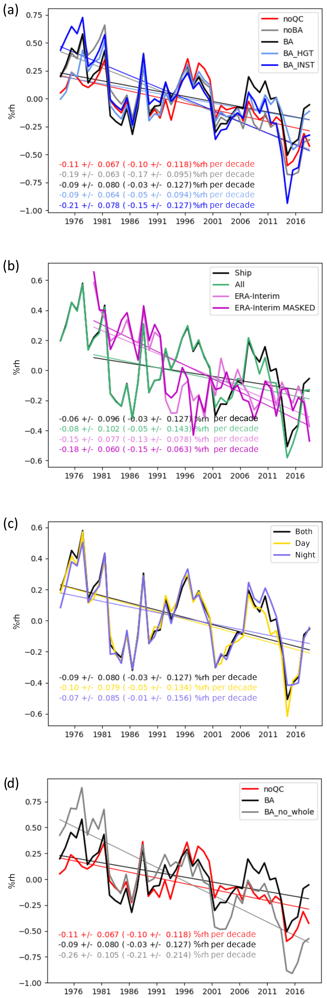
Figure 9 Global annual average anomaly time series and decadal trends (±90 % confidence interval) for relative humidity. See Fig. 8 caption for details. In addition, panel (d) shows the time series from the bias-adjusted data with removal of any data with a whole-number flag set (BA_no_whole). Trends in (b) cover the common 1979–2018 period, and all trends in parentheses cover the 1982–2018 period.

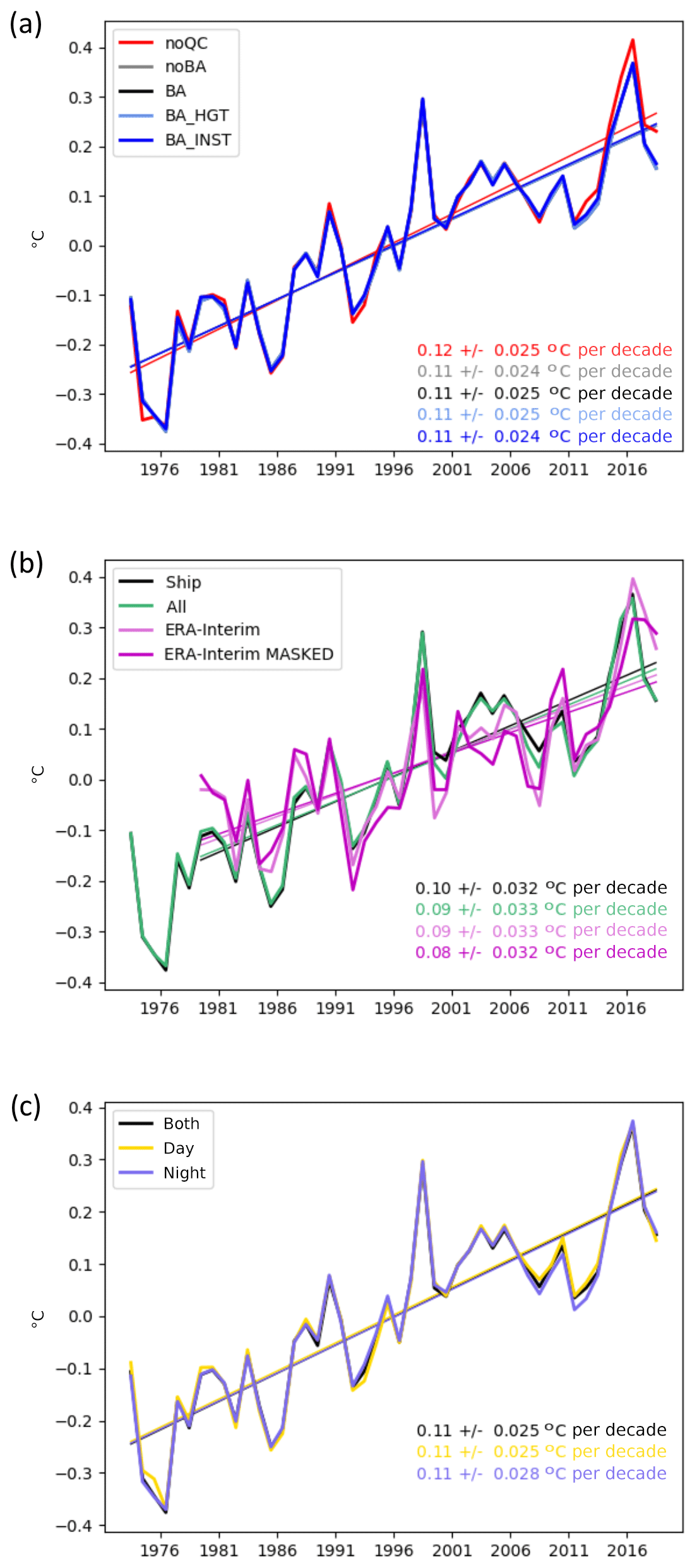
Figure 10 Global annual average anomaly time series and decadal trends (±90 % confidence interval) for dew point temperature. See Fig. 8 caption for details. Trends in (b) cover the common 1979–2018 period.

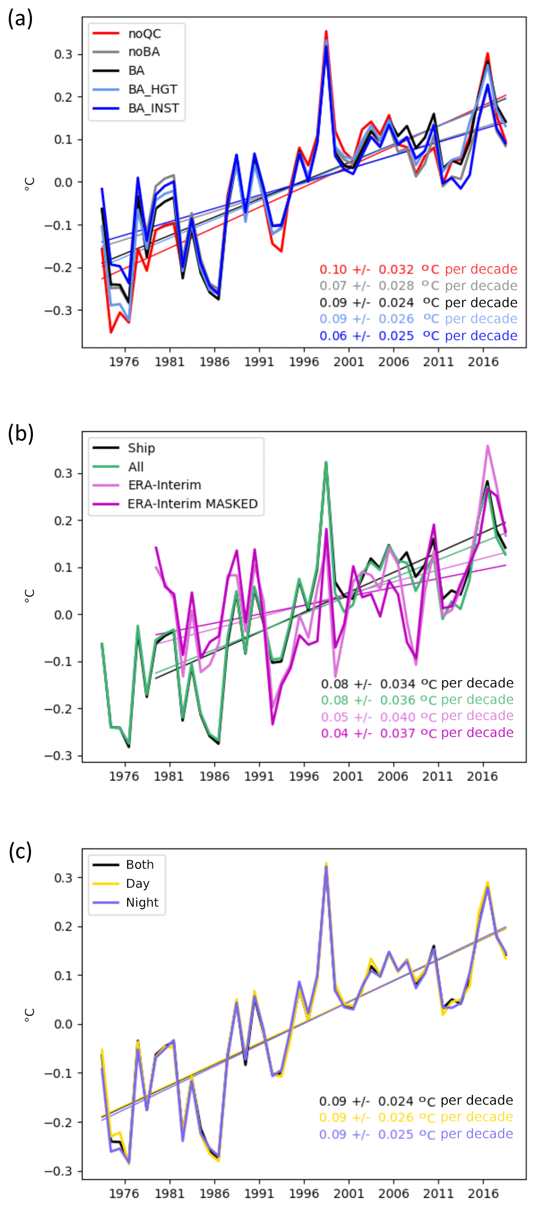
Figure 11 Global annual average anomaly time series and decadal trends (±90 % confidence interval) for marine air temperature. See Fig. 8 caption for details. Trends in (b) cover the common 1979–2018 period.

For all variables, there are only small differences in the global-average time series between the various processing steps – from the raw data (noQC) to the third-iteration quality-controlled (noBA: no bias adjustment) and then the bias-adjusted data (BA). They are smallest for air temperature and largest for relative humidity, but all steps result in global-average trends that are significant and in the same direction and have similar inter-annual variability. We consider these trends to be significant because the 90th-percentile confidence intervals around the trend are not large enough to bring the direction of the trends into question. The trends in the global average are positive over the 1973–2018 period for specific humidity, dew point temperature, and air temperature and negative for relative humidity. The linear trends for the final HadISDH.marine.1.0.0.2018f version are 0.07±0.02 g kg⁻¹ per decade, $-\mathrm{0.09}\pm \mathrm{0.08}$ %rh per decade, 0.09±0.02 ^∘C per decade, and 0.11±0.03 ^∘C per decade for specific humidity, relative humidity, dew point temperature, and air temperature, respectively. Hence, we conclude that HadISDH.marine shows moistening and warming since the 1970s globally in actual terms but that the air above the oceans appears to have become less saturated and drier in relative terms. This differs from the theoretical expectation that changes in relative humidity over ocean are strongly energetically constrained to be small, of the order of 1 % K⁻¹ or less, and generally positive (Held and Soden, 2006; Schneider et al., 2010). Model-based expectations also suggest small positive changes (Byrne and O'Gorman, 2013, 2016, 2018). Despite careful quality control and bias-adjustment, the previously noted moist humidity bias pre-1982 is still apparent in the bias-adjusted (BA) data. The linear trend in relative humidity from 1982 to 2018 is $-\mathrm{0.03}\pm \mathrm{0.13}$ %rh per decade and therefore not significantly decreasing, which is more consistent with expectation.

Since there are considerable known issues affecting the marine humidity data and because there are large outliers (Figs. S3 to S6), the effect of quality (noQC compared to noBA) might be expected to be large. Furthermore, approximately 25 %, dropping steadily over time to 18 %, of the initial selection of data has been removed by the quality control (Fig. 5), so there is a considerable difference in the amount of data contributing to the quality-controlled version compared to the raw version. Despite all of this, differences are relatively small. Overall, the quality control makes the positive trends smaller (specific humidity, dew point temperature, and air temperature) and negative trends larger (relative humidity). The effect of quality control, including buddy checking, is largest in the 1970s to early 1980s, when the largest number of data was removed by quality control. This is especially noticeable for relative humidity and dew point temperature, suggesting that the pre-1982 bias, although present to some extent in the raw (noQC) data, could be exacerbated by the quality control. This could be due to erroneous removal of good data, but investigation (Figs. S3 to S8) suggests that much of the data removal was appropriate; many very low relative-humidity values were removed. It could also be an artefact of the reduced number of observations after quality control, reducing the chance of averaging out random error. To explore whether the presence of whole numbers in the record has contributed to the pre-1982 bias, we have processed a bias-adjusted version with all whole-number flagged data (Table 1) removed (BA_no_whole), which is shown against the noQC and BA versions in Fig. 9d. The resulting global-average trend is largest in the BA_no_whole version, even over the 1982–2018 period, and the pre-1982 bias is still clear. We conclude that the pre-1982 moist bias remains apparent in HadISDH.marine and is not yet well understood, and quality control of the pre-1982 data is an area for more research in future versions.

The bias adjustment (BA, BA_HGT, BA_INST) reduces the negative trends in relative humidity compared to the quality-controlled (noBA) data and increases the positive trends in specific humidity and dew point temperature relative to the quality-controlled data. The effect of bias adjustment is negligible for air temperature, which only has adjustment for ship height applied. For the humidity variables the height adjustment has a far larger effect than the non-aspirated-instrument adjustment. The non-aspirated-instrument adjustment makes the positive trends in specific humidity and dew point temperature slightly smaller and the negative trends in relative humidity slightly larger. The height adjustment has the opposite effect. For relative humidity, the bias adjustments appear to have introduced greater intra-decadal-scale variability but retained the inter-annual patterns, again highlighting the sensitivity of relative humidity compared to the other variables. Given that these biases exist we do have to try and mitigate their impact. However, this is a focus area for investigation and improvements in future versions of HadISDH.marine.

The time series that include data from moored buoys compared to those from ships only (“all” versus “ship”) show smaller positive trends for specific humidity and air temperature and larger negative trends for relative humidity. Moored buoys begin to play a role from the late 1980s, increasing in number dramatically to make up over 50 % of the observations by 2015. The “all” time series can be seen to diverge slightly from the “ship” time series in the latter part of the record. Therefore, it is more consistent to produce the final HadISDH.marine version without inclusion of moored-buoy data.

Before quality control there are more daytime ship observations than night-time ship observations in the early record (∼1 000 000 compared to ∼800 000 yr⁻¹), but this evens out by the end of the record to ∼900 000 yr⁻¹. However, the quality control removes more daytime observations than night-time observations, especially in the 1970s and 1980s, such that both contribute ∼700 000 observations per year, dipping in the middle of the record. There has been no bias adjustment for solar heating of ships applied in this version of HadISDH.marine, so the daytime data may contain some artefacts of solar heating. If this is a problem it should affect the air temperature and relative humidity but not the dew point temperature or specific humidity (Sect. 2.1). While the full dataset (both) combines both daytime and night-time data, for various grid boxes and seasons there is only either a daytime or night-time value present. As such, the “both” time series and its linear trend may not be a straightforward average of the “day” and “night” time series and trends. For specific humidity, dew point temperature, and air temperature, the “day” and “night” trend differences are essentially negligible, with linear trends identical or within 0.01 g kg⁻¹ per decade. Even for relative humidity the differences are small. The “day” time series gives the largest negative trend, followed by “both”, which is 0.01 %rh per decade smaller, and then “night”, which is 0.02 %rh per decade smaller again. The negligible differences in air temperature suggest that solar heating is not a significant concern, at least at the global-average scale. Relative humidity is very sensitive to any differences in the data, but even these differences are fairly small and do not change the overall conclusion of decreasing full-period trends and no significant trend over the 1982–2018 period. “Night” trends are often thought to provide a better signal of change because they are generally free from convective and shortwave radiative processes and more a measure of outgoing longwave radiation. The main conclusion here is that trends and variability are very similar in the daytime, night-time, and combined time series, which adds confidence in their representativeness of real-world trends and variability.

In terms of linear trend direction, HadISDH.marine compares well with other monitoring estimates from NOCSv2.0 and ERA-Interim and to other reanalyses and older products (Fig. 1). ERA-Interim in Figs. 8 to 11 is from analysis fields of 2 m air temperature and dew point temperature and has been masked to ocean coverage using a $\mathrm{1}{}^{\circ }\times \mathrm{1}{}^{\circ }$ land–sea mask and also to HadISDH.marine coverage for comparison. Note that the ERA-Interim time series shown in Fig. 1 are from background forecast values to avoid biases introduced from ship data and ocean-only points over open sea. Both NOCSv2.0 and HadISDH.marine are estimates of 10 m quantities, and the NOCSv2.0 coverage is similar to that of HadISDH.marine, but it only extends to 2015. NOCSv2.0 shows the largest trends in specific humidity over the 1979–2015 common period, 0.04 g kg⁻¹ per decade greater than HadISDH.marine. The inter-annual patterns are broadly similar but with some differences showing that methodological choices do make a difference given that the underlying observations are from the same source. ERA-Interim shows very weak moistening compared to HadISDH.marine for specific humidity and dew point temperature and slightly weaker warming for air temperature. Over the longer 1979–2018 period, ERA-Interim trends are slightly larger for specific humidity but still weaker than in HadISDH.marine. The decreasing saturation in relative humidity is very strong in ERA-Interim, at more than 2 times the HadISDH.marine trend over the common period. The masking to HadISDH.marine coverage surprisingly makes very little difference in the linear trends; they are slightly more negative and only small year-to-year differences. Inter-annual behaviour does differ, especially for relative humidity and especially in the period up to the early 1990s, where ERA-Interim is warmer and wetter generally, thus moderating the long-term trends in specific humidity, dew point temperature, and air temperature. Note that the ERA-Interim background field relative humidity shown in Fig. 1 also shows a decrease but to a lesser extent than the analysis fields (Fig. 9) which include ship data. Agreement is closest for air temperature in both trends and variability.

The decreasing relative-humidity trends over ocean are similar to the drying seen in HadISDH.land and ERA-Interim land relative humidity (Fig. 1); land linear trends are 0.03 %rh more negative, at −0.12 (−0.27 to −0.03) %rh per decade, over the same 1973–2018 period. The time series pattern is quite different though with marine relative humidity decreasing throughout the period around large variability and land relative humidity clearly decreasing from 2000. The greater sensitivity of relative humidity to observation errors, biases, and sampling issues makes the conclusion of long-term drying an uncertain one, but agreement with ERA-Interim adds some weight to this conclusion.

For the final HadISDH.marine.1.0.0.2018f product, the regional-average uncertainty is also computed and shown for the global average (70^∘ S to 70^∘ N) in Fig. 12. This includes the total observation uncertainty, which covers uncertainty components for instrument adjustment, height adjustment, measurement, climatology, and whole-number uncertainty (Table 2). In addition, the regional-average uncertainty includes the grid box sampling uncertainty and also a spatial-coverage uncertainty following the method applied for HadISDH.land (Willett et al., 2014). The coverage uncertainty essentially uses the variability between ERA-Interim full coverage compared to ERA-Interim with HadISDH.marine coverage to estimate uncertainty. To obtain uncertainty in the global average from the grid box uncertainties, correlation in time and space should be taken into account. It is not trivial to assess the true spatial and temporal correlation of the various uncertainty sources. In reality, although ships move around over space and time, implying some correlation, the contributing sources to each ∼500 km² grid box monthly mean differ widely. Therefore, for this first-version product we assume no correlation between grid boxes in time or space and take the simple approach of the quadrature combination of uncertainty sources, noting that this is a lower limit on uncertainties.

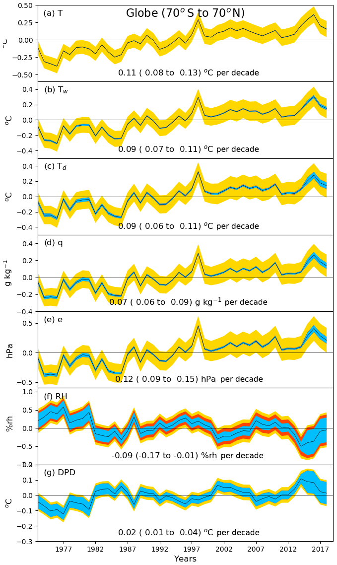
Figure 12 Global-average time series of annual mean climate anomalies for all variables. The 2σ uncertainty ranges for total observation (blue), sampling (red) and coverage (gold) uncertainty contributions combined are shown. All series have been given a zero mean over the common 1981–2010 period. Decadal linear trends and 90th-percentile confidence intervals (in parentheses) were fitted using ordinary least-squares regression with AR(1) correction applied when calculating the confidence intervals (Santer et al., 2008), with the range representing the 90 % confidence interval in the trend.

The uncertainty in the global averages (Fig. 12) is larger than the equivalent time series for land (see Fig. 12 in Willett et al., 2014). The coverage uncertainty (accounting for observation gaps in space and time) is generally the largest source of uncertainty with the exception of relative humidity and dew point depression. For the latter two, the total observation uncertainty makes up the greatest contribution. In all cases the total observation uncertainty is larger at the beginning and especially the end of the records, where there are fewer or no metadata with which to apply bias adjustments. The contribution from sampling uncertainty (grid box spatial and temporal coverage) is generally very small except for relative humidity. This is as expected as the correlation decay distance of humidity should generally be larger over ocean than over land given the homogeneous surface altitude and composition. Overall, the magnitudes of the uncertainties are small relative to the magnitudes of long-term trends and variability in all variables except for relative humidity and dew point depression. This suggests that there is good confidence in changes in absolute measures of humidity over ocean (e.g. specific humidity) and also air temperature but lower confidence in changes in the relative humidity. The warming and moistening are further corroborated by strong theoretical reasoning based on laws of physics governing the expectation that specific humidity should have increased over the period of record given the warming of the oceans and atmosphere that has occurred (Hartmann et al., 2013). The uncertainty model makes many assumptions over correlation of uncertainty in space and time. It is likely that we have overestimated the uncertainty at the grid box scale by assuming complete correlation for height adjustment uncertainty, instrument adjustment uncertainty, and climatological uncertainty. Conversely, we have likely underestimated the uncertainty at the regional-average level by assuming no correlation. This is certainly an area for improvement in future versions.

4.3 Decadal trends across the globe presented by HadISDH.marine

Figure 13 shows the decadal linear trends for specific humidity, relative humidity, dew point temperature, and air temperature for HadISDH.marine.1.0.0.2018f. The completeness criterion for trend fitting is 70 %, more strict than for the climatologies (Fig. 7). This results in poorer spatial coverage especially in the Southern Hemisphere. Clearly, there are no data points outside 70^∘ S to 70^∘ N; hence the restriction of the global-average time series to this region is sensible. The tropical and Southern Hemisphere Pacific Ocean and Southern Hemisphere Atlantic Ocean have virtually no data coverage. Overall, the appearance of the trends shows good spatial consistency, with few grid boxes standing out as obviously erroneous. There has been no interpolation across grid boxes that would have smoothed out any outliers, and so the lack of these outlying grid boxes suggests that the data are of reasonable quality for this long-term analysis at least. Trends are as expected from the global-average time series – generally moistening and warming but becoming less saturated. The same is true over land (Willett et al., 2014).

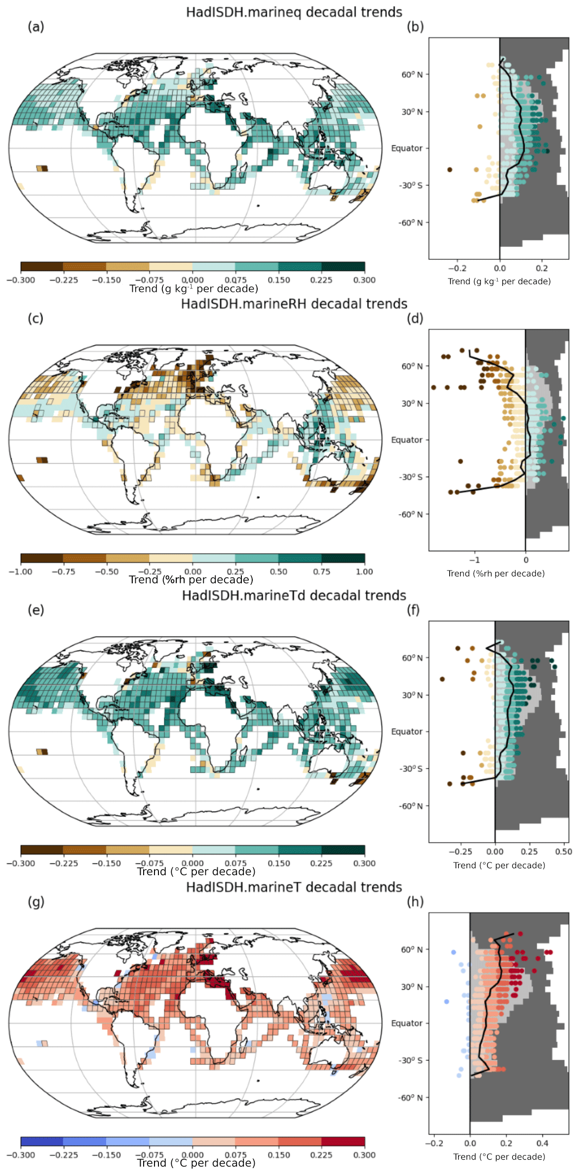
Figure 13 Linear decadal trends from 1973 to 2018 for (a, b) specific humidity (g kg⁻¹), (c, d) relative humidity (%rh), (e, f) dew point temperature (^∘C), and (g, h) air temperature (^∘C) for the third-iteration quality-controlled and bias-adjusted ships only. Decadal linear trends were fitted using ordinary least-squares regression when there are at least 70 % percent of months present over the trend period. Grid boxes with boundaries show significant trends in that the 90 % confidence interval (calculated with AR(1) correction following Santer et al., 2008) around the trend magnitude is the same sign as the trend and does not encompass 0. The right-hand panels (b, d, f, h) show the distribution of grid box trends by latitude with the mean shown as a solid black line. The dark grey shading shows the proportion of the globe at that latitude which is ocean. The light grey shading shows the proportion of the globe that contains observations.

The moistening shown in specific humidity and dew point temperature (Fig. 13a, b, e, and f) is widespread. The majority of grid boxes are considered to be statistically significant in that the 90th-percentile confidence interval around the trend magnitude is the same sign as the trend and does not encompass 0. The largest increases in specific humidity are in the lower latitudes, whereas the largest increases in dew point temperature are more spread out, with a tendency towards the extratropics and mid-latitudes. There are a few regions where there are clusters of grid boxes with drying trends. These are generally consistent between the specific humidity and dew point temperature, especially in the few cases where these negative trends are significant such as the central Pacific, the east coast of Brazil, the southern coast of Australia, and around New Zealand.

Marine air temperature shows widespread and significant warming, in agreement with HadNMAT2 (Kent et al., 2013). Very few of the grid boxes with a negative trend are significant. In some cases they are in similar locations to the drying trends seen in specific humidity and/or dew point temperature, e.g. the coast south of Australia around Tasmania, and the east coast of Brazil. The warming is stronger in the northern mid-latitudes, with the Baltic, Mediterranean, and Red seas showing particularly strong warming consistent with strongly increasing dew point temperature and specific humidity.

Whilst relative humidity is more sensitive to methodological choices and observational errors, the broad spatially coherent structures to the regions of increasing and decreasing saturation with broad-scale significance are very encouraging in terms of data quality. Furthermore, the drying trends tend to be around the mid-latitudes, while the increasing saturation trends are more around the tropics, as seen over land. We still urge caution in the use of marine relative humidity, but these results collectively suggest that decreasing saturation might be a real feature.

5 Code and data availability

HadISDH.marine is available as $\mathrm{5}{}^{\circ }\times \mathrm{5}{}^{\circ }$ gridded fields of monthly means and anomalies along with a 1981–2010 climatology and uncertainty estimates at the grid box scale. The data begin in January 1973 and continue to December 2018 (at the time of writing) and will be updated annually. HadISDH.marine is publicly available from https://www.metoffice.gov.uk/hadobs/hadisdh/ (last access: June 2019) under an Open Government license (http://www.nationalarchives.gov.uk/doc/open-government-licence/version/3/, last access: June 2019) as netCDF and text files. Processing code (Python) can also be made available on request. HadISDH.marine data, derived diagnostics, and plots can be found at http://www.metoffice.gov.uk/hadobs/hadisdh (last access: June 2019) and https://doi.org/10.5285/463b2fcd6a264a39b1e3249dab16c177 (Willett et al., 2020). It should be cited using this paper and the following: Willett, K. M., Dunn, R. J. H., Kennedy, J. J., and Berry, D. I. (2020): HadISDH marine: gridded global monthly ocean surface humidity data version 1.0.0.2018f. Centre for Environmental Data Analysis, https://doi.org/10.5285/463b2fcd6a264a39b1e3249dab16c177, 5 August 2020.

This product forms one of the HadOBS (Met Office Hadley Centre Climate Monitoring Observations; http://www.metoffice.gov.uk/hadobs, last access: June 2019) climate monitoring products and will be blended with the HadISDH.land product to create a global land and marine humidity monitoring product. Updates and exploratory analyses are documented at http://hadisdh.blogspot.co.uk (last access: June 2019) and through the Met Office HadOBS Twitter account @metofficeHadOBS.

6 Discussion and conclusions

Marine humidity data are susceptible to a considerable number of biases and sources of error that can be large in magnitude. We have cleaned the data where possible by applying quality control for outliers, supersaturation, repeated values and neighbour inconsistency, which has removed up to 25 % of our initial selection in some years. We have also applied adjustments to account for biases arising from unaspirated instrument types and differing observation heights over space and time. Care has also been taken to avoid diurnal and seasonal sampling biases as far as possible when building the gridded fields, and the use of grid box mean climate anomalies reduces remaining random error through averaging.

Spatial coverage of HadISDH.marine differs year to year. The coverage is generally poorer than seen for variables such as SST which benefit significantly from drifting-buoy observations. Any further decline in observation and transmission of humidity from ships is of concern to our ability to robustly monitor surface humidity over oceans. Future versions may be able to make more use of humidity data from buoys, but their proximity to the sea surface and difficulty of regular maintenance can lead to poor-quality observations. The provision of digital metadata significantly improves our ability to quantify and account for biases in the data. Hence, the continuity of this metadata beyond 2014 and ideally an increase in quantity also strongly affect our ability to robustly monitor ocean surface humidity. Given the current availability of ship data and metadata as well as the necessarily strict selection criteria and quality control, the resulting spatial coverage is good over the Northern Hemisphere outside of the high latitudes. There is very poor coverage over the Southern Hemisphere, especially south of 20^∘ S. This means that our “global” analyses are biased to the Northern Hemisphere. Care should be taken to account for different spatial coverage when comparing products. However, when comparing HadISDH to masked and unmasked ERA-Interim fields, differences were surprisingly small.

We have shown that the observations are warm and moist relative to ERA-Interim reanalysis for the majority of the observed globe apart from the north-western Pacific. This is despite ERA-Interim fields representing 2 m above the surface compared to the general observation heights of 10–30 m above the surface. Differences are largest around coastlines, particularly in the Red Sea and Persian Gulf. There is insufficient spatial coverage to produce a high-resolution climatology from the data themselves, hence our use of ERA-Interim initially and then interpolated observation-based fields. However, the lower-resolution ($\mathrm{5}{}^{\circ }\times \mathrm{5}{}^{\circ }$) monthly mean climatologies from the final HadISDH.marine.1.0.0.2018f version show expected spatial patterns and have good spatial consistency, providing evidence that our data selection methods have resulted in reasonably high-quality data.

The quality control and bias adjustment procedures have made small differences to the global-average-anomaly time series for specific humidity, dew point temperature, and air temperature. This overall agreement in the global-average time series between versions and also between the daytime, night-time, and combined versions increases confidence in the overall signal of increased moisture and warmth over oceans. These features show widespread spatial consistency in the HadISDH.marine.1.0.0.2018f grid box decadal trends, which also adds confidence. Hence, we can conclude that the ICOADS data are a useful source of humidity data for climate monitoring. However, we expect differences to be larger in smaller-spatial-scale analyses. HadISDH.marine shows consistency with other products in terms of long-term linear trends in the global averages. There are some differences year to year, with ERA-Interim showing warmer and moister anomalies prior to the early 1990s and hence smaller trends overall.

For relative humidity, differences between the versions can be large for any one year, but the overall decreasing saturation trend appears to be robust. We conclude this because the trend is consistent across all processing steps, is apparent in ERA-Interim fields, and also has spatial consistency across the extratropics and mid-latitudes. This is a somewhat surprising result and one that should be treated cautiously. Theoretical and model-based analysis of changes in relative humidity over ocean under a warming climate suggests negligible or small positive changes (Held and Soden, 2006; Schneider et al., 2010; Byrne and O'Gorman, 2013, 2016, 2018). The temporal patterns in global-average relative humidity are quite different to those over land, whereas specific humidity shows similarity with the HadISDH.land time series, largely driven by the El Niño-related peaks. The pre-1982 data have previously been noted as having a moist bias, and our processing steps do not appear to have removed this feature. The trend excluding this earlier period (1982–2018) is no longer a significant decreasing trend and is therefore more consistent with expectation. Removal of whole-number flagged data appeared to exacerbate the pre-1982 bias and make the negative trends larger. Further work to assess the physical mechanisms that might lead to such trends is needed.

There are known issues with ERA-Interim in terms of its stability. For example, sea surface temperatures cooled around mid-2001 due to a change in the SST analysis product used (Simmons et al., 2014). This is very likely to affect humidity over the ocean surface in ERA-Interim. Similarly, changes in satellite streams over time can also affect the long-term stability of ERA-Interim, even in the surface fields. Also, the assimilated ship data are not adjusted for biases in the ERA-Interim assimilation. Clearly, there are various issues affecting both in situ monitoring products and reanalysis products such that neither one can be easily identified as the more accurate estimate. Analyses should take into account all available estimates and their strengths and weaknesses. Comparison of HadISDH.marine with satellite-based estimates of humidity over ocean will be an important next step.

We have attempted to quantify uncertainty in HadISDH.marine. The uncertainty analysis comprises observation uncertainty at the point of measurement, which is then propagated through to grid box averages, taking correlation in space and time into account where relevant. Sampling uncertainty at the grid box level due to uneven sampling across the grid box in space and time is assessed. We have also provided uncertainty estimates in regional and global averages including coverage uncertainty. The propagation of grid box observation and sampling uncertainty to large-scale averages does not explicitly take into account correlation in these uncertainty quantities in space and time. As this is a first-version monitoring product, this simple method is seen as an appropriate first attempt to assess uncertainty. The ranges presented should be seen as a lower limit on the uncertainty. Overall, uncertainty in the global average is dominated by the coverage uncertainty for all variables except relative humidity and dew point depression. The total observation uncertainty is larger at the beginning and especially the end of the record, where digital metadata are fewer or non-existent (post-2014). Overall, the uncertainty is small relative to the magnitude of long-term trends with the exception of relative humidity. We suspect that this is an overestimate at the grid box level owing to assumptions of complete correlation in the height adjustment, instrument adjustment, and climatology uncertainty components and an underestimate at the regional-average level given assumptions of no correlation. This is a first attempt to comprehensively quantify marine humidity uncertainty, and future methodological improvements are envisaged.

We conclude that this first-version marine humidity monitoring product is a reasonable estimate of large-scale trends and variability and contributes to our understanding of climate changes as a new and methodologically independent analysis. The trends and variability shown are mostly in concert with expectation; widespread moistening and warming are observed over the oceans (excluding the mostly data-free Southern Hemisphere) from 1973 to present. These are also large relative to the magnitude of our uncertainty estimates. Our key finding is that the marine relative humidity appears to be decreasing (the air is becoming less saturated). We have explored various processes for ensuring high-quality data and shown that these do not make large differences for large-scale analyses of specific humidity, dew point temperature, and air temperature but that there is greater sensitivity to methodological choices for relative humidity.

The spatial coverage of surface humidity data is very low outside of the Northern Hemisphere. If only those data with digitized metadata are included then this coverage deteriorates further. Although moored-buoy numbers have increased dramatically since the 1990s, their measurements are more prone to error through proximity to the water and hence contamination in addition to less frequent manual checking and maintenance. Hence, our ability to monitor surface humidity with any degree of confidence depends on the continued availability of ship data and provision of digitized metadata.