the Creative Commons Attribution 4.0 License.
the Creative Commons Attribution 4.0 License.
 | 12 Nov 2020
Physical and biogeochemical parameters of the Mediterranean Sea during a cruise with RV Maria S. Merian in March 2018
Dagmar Hainbucher
Marta Álvarez
Blanca Astray Uceda
Giancarlo Bachi
Vanessa Cardin
Paolo Celentano
Spyros Chaikalis
Maria del Mar Chaves Montero
Giuseppe Civitarese
Noelia M. Fajar
Francois Fripiat
Lennart Gerke
Alexandra Gogou
Elisa F. Guallart
Birte Gülk
Abed El Rahman Hassoun
Nico Lange
Andrea Rochner
Chiara Santinelli
Tobias Steinhoff
Toste Tanhua
Lidia Urbini
Dimitrios Velaoras
Fabian Wolf
Andreas Welsch
The last few decades have seen dramatic changes in the hydrography and biogeochemistry of the Mediterranean Sea. The complex bathymetry and highly variable spatial and temporal scales of atmospheric forcing, convective and ventilation processes contribute to generate complex and unsteady circulation patterns and significant variability in biogeochemical systems. Part of the variability of this system can be influenced by anthropogenic contributions. Consequently, it is necessary to document details and to understand trends in place to better relate the observed processes and to possibly predict the consequences of these changes. In this context we report data from an oceanographic cruise in the Mediterranean Sea on the German research vessel Maria S. Merian (MSM72) in March 2018. The main objective of the cruise was to contribute to the understanding of long-term changes and trends in physical and biogeochemical parameters, such as the anthropogenic carbon uptake and to further assess the hydrographical situation after the major climatological shifts in the eastern and western part of the basin, known as the Eastern and Western Mediterranean Transients. During the cruise, multidisciplinary measurements were conducted on a predominantly zonal section throughout the Mediterranean Sea, contributing to the Med-SHIP and GO-SHIP long-term repeat cruise section that is conducted at regular intervals in the Mediterranean Sea to observe changes and impacts on physical and biogeochemical variables. The data can be accessed at https://doi.org/10.1594/PANGAEA.905902 (Hainbucher et al., 2019), https://doi.org/10.1594/PANGAEA.913512 (Hainbucher, 2020a) https://doi.org/10.1594/PANGAEA.913608, (Hainbucher, 2020b) https://doi.org/10.1594/PANGAEA.913505, (Hainbucher, 2020c) https://doi.org/10.1594/PANGAEA.905887 (Tanhua et al., 2019) and https://doi.org/10.25921/z7en-hn85 (Tanhua et al, 2020).
- Article
(10066 KB) - Full-text XML
- BibTeX
- EndNote


Repository Reference. Table 1a and b and list of available data sets (Table 1c).
Table 1(a) List of physical parameters from Maria S. Merian cruise MSM72 as seen in the PANGAEA database. The primary investigator was Dagmar Hainbucher. (b) List of biogeochemical parameters from Maria S. Merian cruise MSM72 as seen in the CCHDO database. The primary investigator was Toste Tanhua. (c) List of available data sets.
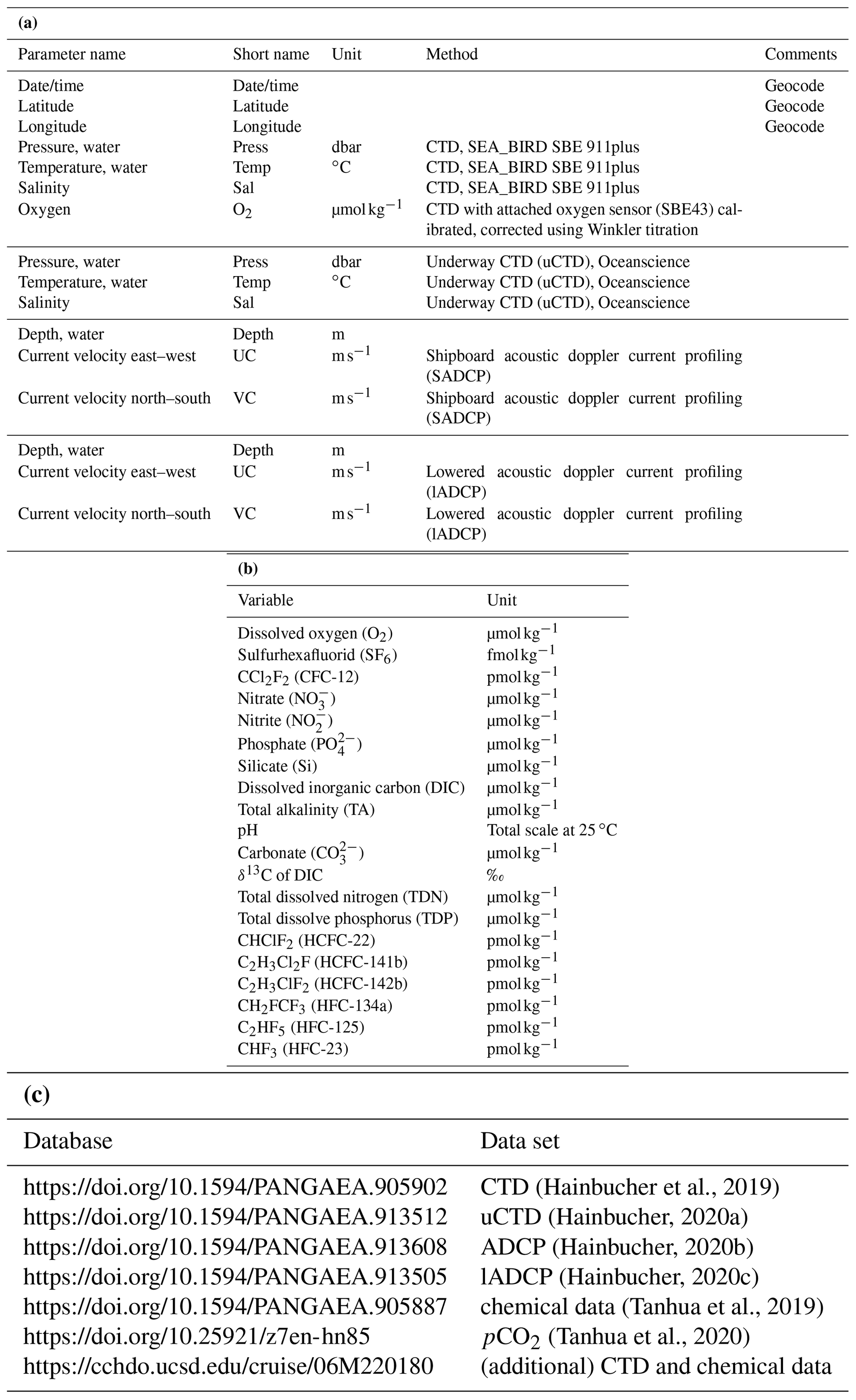
A link to the summary page of the cruise MSM72 can be found in the PANGAEA
database under https://www.pangaea.de/?q=msm72&f.campaign%5B%5D=MSM72 (last access: 10 November 2020).
Coverage. 34–41∘ N, 6∘ W–28∘ E
Location name. The Mediterranean Sea
Date/Time start. 2 March 2018
Date/Time end. 3 April 2018
Contrary to earlier ideas that the Mediterranean Sea is always in a steady state, we now know in the light of new research that the Mediterranean Sea is not, and it is potentially sensitive to climatic changes (Malanotte-Rizzoli, 2014). Proving this are the drastic changes that the eastern Mediterranean (EMed) has undergone in the past. The largest climatic event, named the Eastern Mediterranean Transient (EMT), occurred in the EMed between the late 1980s and early 1990s, where deep-water formation switched from the Adriatic Sea to the Aegean Sea. This episode modified the thermohaline characteristics of the outflow through the Sicilian Strait, advecting anomalously salty and warm Levantine Intermediate Water (LIW) to the western Mediterranean Sea (WMed) and leading to a significant increase in temperature and salt in the intermediate and deep layers of the WMed. Additionally, strong deep convection induced by extreme atmospheric events during winter in 2004–2006 (low precipitation, cold, persistent winds) also enhanced salt and temperature in the entire basin up to about 1600 m (Schroeder et al., 2006, 2008). This abrupt climate shift is referred to as Western Mediterranean Transient (WMT) and the physical changes are comparable to the EMT, both in terms of intensity and observed effects (Schroeder et al., 2008). The existence of both transients contradicts the hypothesis of a steady state. On the other hand, it has also been proven that an EMT has never been observed before (Roether et al., 2013).
The characteristic of the Mediterranean Sea is also such that it has the potential to sequester large amounts of anthropogenic CO2, Cant, since the Mediterranean Sea has high alkalinity and temperature, which can be rapidly transported to deep by the overturning circulation (e.g., Schneider et al., 2010). The column inventories of Cant in the Mediterranean are among the highest found in the world oceans; the Mediterranean Sea thus stores a significant portion of the global anthropogenic emissions of Cant despite its relatively small volume.
Furthermore, marine dissolved organic carbon (DOC) represents the largest reservoir of reduced carbon (662×1015 g C) on Earth (Hansell, 2009), it therefore plays a major role in the global carbon cycle. Its role in the functioning of marine ecosystems is equally crucial since DOC is released at all the levels of the food web as a byproduct of many trophic interactions and/or metabolic processes and is the main source of energy for the heterotrophic prokaryotes (Carlson and Hansell, 2015). Although most of DOC is produced in situ, external sources (atmosphere, rivers, sediments) may affect its concentration and distribution. Physical processes, such as deep-water formation, thermohaline circulation, vertical stratification and mesoscale activities have been reported to be the main drivers of DOC distribution in the Mediterranean Sea (Santinelli, 2015; Santinelli et al., 2015, 2013).
The main scientific objective of the cruise reported here was to add knowledge to the different scales and magnitudes of variability and trends in circulation, hydrography, and biogeochemistry of the Mediterranean Sea. Key variables were measured in strategic regions in order to understand changes, the reason for occurrence, and the drivers. In this context, this cruise is part of the Med-SHIP and GO-SHIP long-term repeat cruise section that is conducted at regular intervals in the Mediterranean Sea to observe changes and impacts on physical and biogeochemical variables.
The following science questions are addressed in this work.
-
What are the long-term changes and/or trends in physics and biochemistry in the Mediterranean Sea, including all the sub-basins?
-
How is the hydrographic situation in the Mediterranean developing further following the EMT and WMT? Is there still a tendency of the system to return to the pre-EMT situation and is there a similar trend in the WMed?
-
How are eddies distributed in the EMed and WMed during the cruise? Do they differ in the sub-basins? To what extent is heat and salt transferred into the vertical by eddies in the WMed and EMed during the cruise period?
-
What is the uptake rate of the anthropogenic carbon in the Mediterranean and is this changing over time?
-
What is the extent of the variability and trends in the inventory of biogeochemical variables (including oxygen, nutrients and dissolved organic carbon)?
-
What are the baseline values of rarely measured essential ocean variables (EOVs) such as dissolved organic carbon (DOC)?
The survey was carried out on the German RV Maria S. Merian from 2 March to 3 April 2018. The cruise started on Heraklion, Greece, and ended in Cádiz, Spain. The main focus of the cruise was on an east–west transect across the western and eastern Mediterranean Sea (Fig. 1) starting east of Crete and ending near the Strait of Gibraltar, which is a repeating hydrographic line in GO-SHIP (MED1). Difficulties with diplomatic authorizations for Marine Scientific Research (MSR) in the area east of Crete made it impossible for us to carry out our measurements as initially planned, and thus no data were obtained east of the Kasos Strait.

Figure 1Station map. Yellow dots are CTD without any chemical sampling, red dots are CTD with chemical sampling, cyan dots are CTD with chemical and additional sampling of isotopes, yellow squares are the deployment of drifter and floats, blue lines are fine resolved uCTD and ADCP tracks, and black lines are tracks with uCTD casts between CTD stations. (a) Detail of the central map of the western Mediterranean Sea. (b) Detail of the central map of the eastern Mediterranean Sea. (c) Detail of the central map of the Otranto Strait and northern Ionian Sea. (d) Detail of the central map of the Tyrrhenian Sea and Sicilian Strait.
During the 33 d of the cruise we carried out measurements of hydrographic and biogeochemical variables along track with the classical approach, i.e., CTD, lADCP, uCTD instrumentation and bottle samples on highly resolved sections across the Mediterranean Sea. The high resolution of CTD stations, enhanced for the physical parameters by additional uCTD measurements, allowed us to resolve the eddy field on the sections; the analysis was also supported and complemented by satellite data.
Most sections and CTD-positions follow previous sampling strategies (cruise M84 and others along the GO-SHIP line MED-01, i.e., Tanhua et al., 2013) to allow long-term trend analyses. Along the different sections, CTD stations including sampling of chemical parameters were conducted approximately every 30 nm, CTD without sampling about every 15–20 nm and with even smaller spacing in the straits. In addition, underway CTD measurements and ADCP measurements were performed between CTD stations.
The water sampling program included measurements of all level 1 variables as defined by GO-SHIP (i.e., oxygen, macronutrients, transient tracers and the carbonate system, http://www.go-ship.org/DatReq.html, last access: 10 November 2020) and measurements of the biogeochemical EOVs 13C, nitrous oxide (N2O) and dissolved organic carbon (DOC). These data were used to quantify trends and variability of ventilation and biogeochemical cycles, in particular uptake of anthropogenic carbon.
Sections were additionally conducted through the important passages of the Otranto Strait, Kasos Strait, Antikythera Strait, Sicilian Strait and Strait of Gibraltar, in order to characterize the incoming and outgoing flows. CTD stations in the eastern Ionian Sea were carried out to quantify the flow of the Levantine Surface Water (LSW) into the Adriatic Sea and to track the outflow of the Adriatic Deep Water (AdDW) into the Ionian Sea.
3.1 CTD rosette
All together 136 CTD casts were performed, from which 18 were catalogued as isotopic (a full suite of observations is given in Table 1a and b), 65 as chemical (i.e., GO-SHIP level 1 variables) and 59 as physical (i.e., only sampling for salinity). Due to the water amount needed, two casts were performed on most of the isotopic stations, the first cast was a full profile and the second a shallow one. During the physical stations, water samples at three levels were taken for salinity analysis. The samples were then analyzed on board using a Guildline Autosal Salinometer. A total of 162 samples in 59 stations were taken during the cruise with an offset with respect to standard water varying from 0.0002 to 0.0030 depending on the laboratory temperature. The samples were taken at depth with a constant salinity gradient to ensure that no natural changes in salinity affect the comparison between sample and sensor.
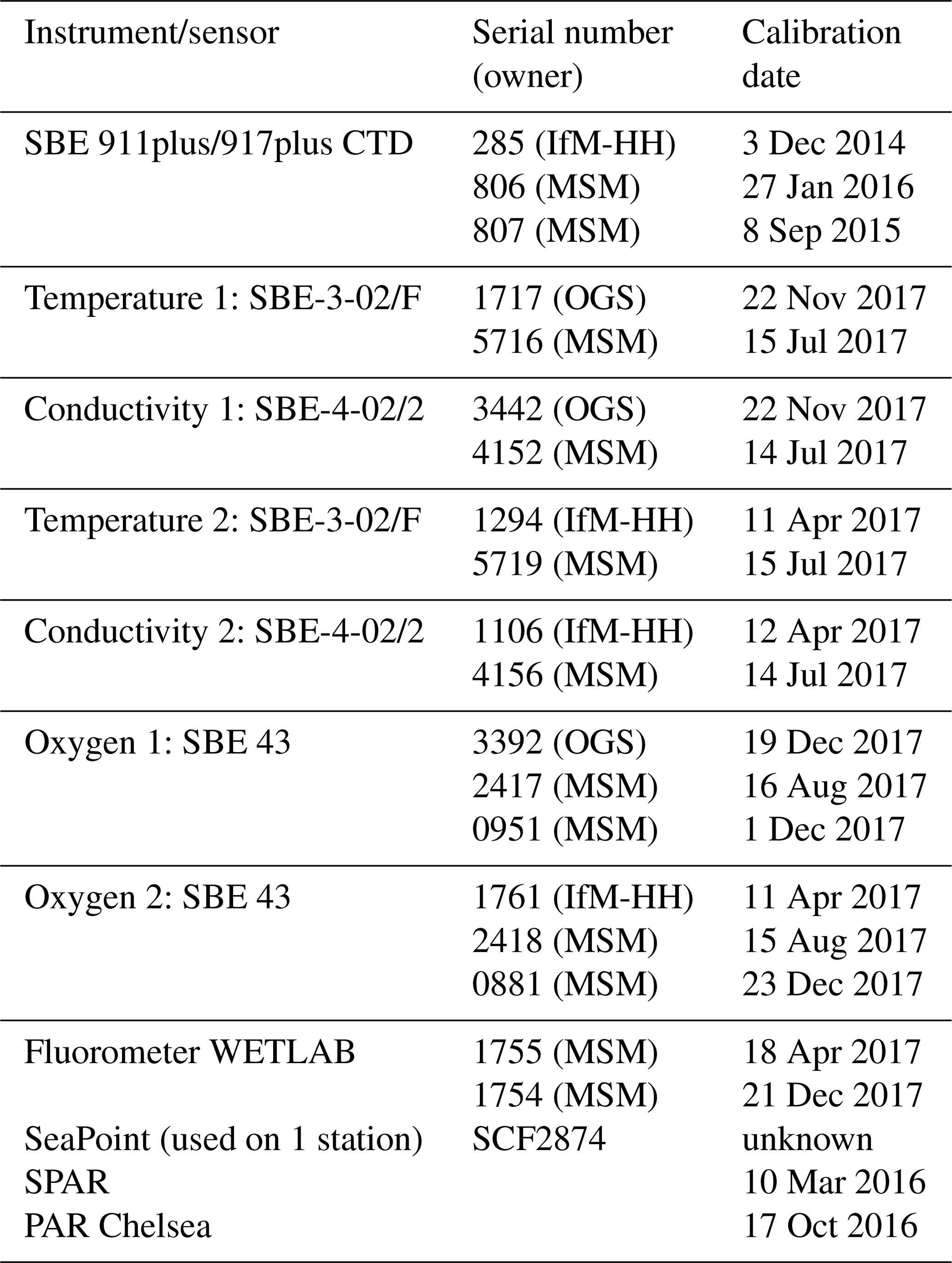
The primary CTD system (for specifications, see Table 2) initially used on board was a Seabird SBE9plus + CTD s/n 0285 from the University of Hamburg connected to a SBE11 deck unit, configured with a 24-position SBE-32 pylon (from GEOMAR) with 10 L Niskin bottles. The position of bottle no. 23 and no. 24 was occupied by the lADCP (for specifications, see Table 3). Initially, the CTD was set up with two sensors for temperature and conductivity, an oxygen sensor, a fluorometer, and an altimeter. To test the configuration and performance of the instrument a station was carried out on the Cretan Sea at the start of the cruise. Unfortunately, we had countless problems with instruments, sensors, cables and the rosette during most of the campaign that forced us to change them very often with others available on board, resulting in a continuous change of system configuration. Thus, all different configurations were carefully considered when post-processing the CTD data.
Temperature, salinity and pressure data were post-processed by applying Seabird software and MATLAB® routines. At this stage, spikes were removed and 1 dbar averages calculated. A first attempt to assess the performance of the conductivity sensors installed on the CTD rosette was done by comparing the salinity data with the bottle samples analyzed with the salinometer. The different hardware setups and configurations are taken carefully into account during post-processing. Overall accuracies are within the expected range of salinity (0.003).
Table 2Used CTD instrument and sensors. Owner of instruments are either the University of Hamburg, Germany (IfM-HH); the National Institute of Oceanography and Geophysics (OGS), Italy; or the property of the vessel Merian (MSM).
3.2 Underway CTD
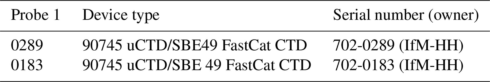
Underway CTD measurements (uCTD; for specifications, see Table 4) provide high-resolution profiles of temperature, conductivity and depth, which allow us to characterize the upper-ocean properties and identify the position and characteristics of mesoscale structures. The advantage of this type of measurement is that it is not required to stop the vessel, it is only necessary to maintain lower velocities (about 3 kn) during the deployments to reach greater depths. These measurements were made with an Ocean Science uCTD system.
The first uCTD deployment was done on 5 March, between CTD 015 and 016 stations, and we continued with this type of sampling between each CTD station to increase the sampling resolution. Unfortunately, several deployments were canceled due to severe weather conditions and no uCTD cast was performed when the depth was shallower than 500 m. All together, 176 casts were taken with depths ranging from 557 to 864 m.
Two probes were used during the cruise with a no-time-limit mode configuration (apart from the first cast configured to stop recording after 600 s, reaching 616 m depth) in order to get longer records. The probe tail spools were attached to the winch through a rope loop that was made new every day in the morning. Despite the probes being able to record several casts, data were downloaded right after each cast using a SBE software in order to avoid losing the data in case the probe was lost and to free up the memory. The probes were exchanged when the battery was running low (around 3.8 V). On three occasions no data were recorded because the magnet was taken off twice before deployment.
For calibration purposes, some additional casts were done right after the CTD cast in order to compare the data sets. The probes were also sent down with the starboard CTD in station 130.
Data files were processed using a set of MATLAB® routines. After extracting the downcast data, the first correction was done to remove inaccuracies in the descent rate, based on the work of Ullmann and Hebert (2014). Additionally, the data were aligned to the comparable CTD data sets.
3.3 lADCP measurements
Ocean currents were studied by means of vertical profiles made with a lADCP-2 system (Workhorse RD Instruments type, Table 3) which included two ADCPs operating at a frequency of 300 kHz, one looking upward and the other one looking downward. The system was placed in the rosette occupying the position of Niskin bottles 23 and 24. During the cruise, the lADCP batteries were changed twice: the first time on 17 March in Station 58 and the second time on 27 March in Station 105. Except for three stations (station 73, 74, 80) with water depths less than 500 m, lADCP measurements were done at all CTDs. For these stations, the currents were observed by the ship-mounted ADCP. At isotope stations, lADCP profiles were only recorded from the deep cast. The gained data were processed with LDEO MATLAB® lADCP processing system version 10.15 (Turnherr, 2014). This software uses the raw lADCP data, processed CTD data and navigational data from the CTD. The resulting data are the u- and v- velocities at the depth. The bin size was set to 8 m.

3.4 Shipborne ADCP
During the whole campaign, underway current measurements were taken with two vessel-mounted Ocean Surveyors (ADCP) manufactured by RDI. The first, with a working frequency of 75 kHz, covered approximately the top 500–700 m of the water column. The number of bins was set to 100 with bin size of 8 m. The second, with a working frequency of 38 kHz, has a depth range of about 1600 m, set with the same bin number as the previous one and bin size of 16 m. Both instruments run in narrowband mode and were controlled by computers using the conventional RDI VMDAS software under a Microsoft Windows system with a pinging set to fast as possible. No interferences with other used acoustical instruments were observed. The ADCP data was post-processed afterwards with the CODAS3 Software System (https://currents.soest.hawaii.edu/docs/adcp_doc/, last access: 10 November 2020), which allows extracting data, assigning coordinates, and editing and correcting velocity data. Moreover, the data were corrected for errors in the value of sound velocity in water, and misalignment of the instrument with respect to the axis of the ship (about −2.8∘ for 75 kHz ADCP and about −0.15∘ for 38 kHz ADCP).
3.5 Underway CO2 and O2 measurements
Underway (UW) measurements of partial pressure of CO2 (pCO2), and dissolved oxygen partial pressure (pCO2 the corresponding data set in Table 1b only contains pCO2) in seawater were carried out by means of a Contros HydroC pCO2 analyzer for pCO2 and an Aanderaa optode for oxygen.
The instruments were placed in a cooling box in the hangar. Seawater was drawn from the ship's centrifugal pump for clean seawater that was continuously flowing through the cooling box with the inlet close to the instruments. Water was pumped through a SeaBird 5 salinity and temperature sensor and onto the HydroC instrument (Gerke, 2020).
The system operated reliably throughout the cruise, except when data acquisition was interrupted for the pCO2 instrument for 2 d directly after the ship's centrifugal pump was switched off. This led to a 5 d period without data between 5 and 10 March. During the cruise, 13 samples were taken from the cooling box for discrete measurements of pH and total alkalinity. The UW measurements started on 2 March at 20:20 and stopped on 1 April 2018, at 14:00 UTC.
The underway oxygen measurements were calibrated by comparing them to the Winkler measurements taken for surface samples at the chemical CTD stations.
3.6 Dissolved oxygen
Dissolved oxygen in seawater was not only measured with the CTD, but samples were also taken at every station and depth along the cruise and reported in µmol kg−1. GO-SHIP guidelines recommend Winkler measurements on all samples, in addition to sensor measurements on the CTD package, and we largely followed those recommendations. Unfortunately, we had to mark large numbers of oxygen values determined with the CTD as questionable due to the several technical problems with the CTDs and sensors. Usually, samples were taken at standard depths, but, especially at the surface and at the bottom, the depths were varied according to the requirements of the other biogeochemical parameters. Oxygen was measured following the automatic Winkler potentiometric method, modified following Langdon (2010). Titrations were done within the sampling calibrated flasks using an Automatic Titrator Mettler Toledo T50 with a platinum combined electrode.
Reagents of blank and thiosulfate standardization were done daily by means of potassium iodate standard 1.667 mmol by OSIL, UK. About 1400 samples were analyzed on board. The precision of dissolved oxygen measurements was determined on five replicates at the beginning and at the end of the cruise (Table 5).
In addition, during the cruise 46 duplicates were analyzed. The results are given in Table 6.
Table 5Precision of dissolved oxygen (SD is standard deviation, and CV is coefficient of variation).

Table 6Results of duplicates.
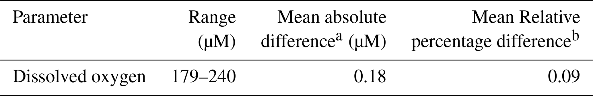
a AD=| duplicate no. 1 − duplicate no. 2|. b RPD % = absolute difference ⋅100 ∕ mean (dupl. no. 1, no. 2).
3.7 Nutrients (nitrite, nitrate, phosphate and silicate), total dissolved nitrogen (TDN) and total dissolved phosphorus (TDP)
3.7.1 Nutrients
Analyses were performed at 40 ∘C on a four-channel, Quaatro SEAL Analytical Continuous Flow Analyzer s/n 8014549; https://www.seal-analytical.com/Products/SegmentedFlowAnalyzers/QuAAtro39AutoAnalyzer/tabid/814/language/en-US/Default.aspx (last access: 10 November 2020), according to Hansen and Koroleff (1999). Nitrite was determined through the formation of a reddish-purple azo dye and measured at 520 nm (SEAL Method no. Q-030-04 Rev. 2). Nitrate was reduced to nitrite in a copperized cadmium reduction coil and then determined as described for nitrite (SEAL Method no. Q-035-04 Rev. 4). The determination of phosphate was based on the reduced blue phospho-molybdenum complex and then measured at 880 nm (SEAL Method no. Q-031-04 Rev. 1). Silicate was determined by means of acidic reduction of silicomolybdate to molybdenum blue and then measured at 820 nm (SEAL Method no. Q-038-04 Rev. 0).
About 1400 nutrient samples were analyzed on board. The onboard precision of nutrient measurements was determined on five replicates at the beginning and at the end of the cruise. The results are shown in Table 7.
In addition, during the cruise 140 duplicates were analyzed. The results are shown in Table 8.
An internal quality check was daily performed by means of analyses of QUASIMEME samples, which provided results within the already certified ranges.

Table 8Analysis of duplicates.

a AD =| duplicate no. 1 − duplicate no. 2|; b RPD % = absolute difference ⋅ 100 ∕ mean (dupl. no. 1, no. 2). c Nitrite statistics was given just for completeness, since the concentration levels recorded were too low and often below the detection limit.
3.7.2 TDN and TDP
About 550 samples for total dissolved nitrogen and total dissolved phosphorus (TDN and TDP) on land-based laboratory analyses were collected and frozen at −20 ∘C after filtration on pre-combusted GF/F filter. The dissolved organic components, dissolved organic nitrogen (DON) and dissolved organic phosphorus (DOP) were subsequently calculated by subtracting their mineral constituents (NO3+NO2) and PO4, respectively.
3.8 Discrete CO2 system measurements
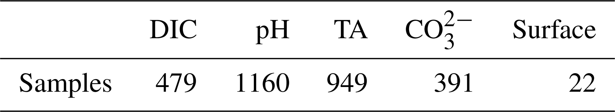
Discrete CO2 variables were measured on board, i.e., dissolved inorganic carbon (DIC), pH, total alkalinity (TA) and carbonate ion (); these variables were measured at selected stations and depths (Table 9). In addition, discrete samples for DIC, pH and TA were analyzed specifically from surface Niskin bottles to be compared with the continuous water supply feeding the pCO2 system in determined stations. For further details, especially about the on-board procedure for the measurement of samples, see Hainbucher et al. (2018).
Table 9Total number of CO2 system samples analyzed during the MSM72 cruise. The total number of fired bottles was 1723.
3.8.1 DIC
Samples for DIC were collected following transient tracers and dissolved oxygen in 500 mL borosilicate bottles following standard procedure. No poison was added. Samples were left at room temperature in the dark until analysis a maximum of 48 h after collection. DIC samples were analyzed with a MARIANDA VINDTA 3D system coupled with a UIC 5011 coulometer. This analysis overall consists of extracting seawater CO2 from a known volume of sample by adding phosphoric acid, followed by coulometric detection (Johnson et al., 1993). No calibration unit was available for the system. A new coulometric cell was prepared for every batch of analysis and the accuracy of the DIC measurements was assessed by using Certified Reference Material (CRM no. 158 and no. 170, provided by Andrew G. Dickson, UCSD). The calibration factor obtained from the CRM was used for adjusting the final DIC of each sample measured in the corresponding batch of analysis. In addition, substandard seawater (stabilized seawater from the Cretan Sea 700 m salinity minimum, stored in the dark in a 30 L container) was analyzed at the beginning and end of the batch analysis as a secondary quality control. The precision of the DIC measurements was checked by (1) double analysis from the same sample and (2) replicate analysis from four to five samples collected from the same Niskin bottle. The precision is estimated to be 1 µmol kg−1, and the accuracy is assumed to be 2 µmol kg−1.
3.8.2 pH
Seawater spectrophotometric pH was measured following Clayton and Byrne (1993) at almost all depths in the chemical and isotope stations during the MSM72 cruise (Table 1). This method consists on adding a volume of indicator solution to the seawater sample, so that measuring the absorbance of the sample at different wavelengths and obtaining the ratio between two of the wavelength's absorbance is proportional to the sample pH. The indicator was a 2 mM solution of unpurified m-cresol purple (Sigma Aldrich®) prepared in seawater and maintained in the dark with no air contact (absorbance ratio of 1.30). Samples were taken following standard procedures immediately after DIC and directly into cylindrical 10 cm path length optical glass cells. The cells were thermostatized at 25±0.2 ∘C for 1 h before analysis. Absorbance measurements were obtained in the thermostated chamber of a double-beam UV 2600 Shimadzu spectrophotometer. The equipment was checked before the cruise for the absorbance and wavelength accuracy using holmium standards. The pH values on the total scale were calculated and referred at 25 ∘C by using the formula by Clayton and Byrne (1993). The injection of the indicator in the sample slightly changes the sample pH. Following standard operating procedures, double additions of the indicator were performed over a pH gradient in order to obtain the corresponding correction (Hainbucher et al., 2018). The pH accuracy was controlled measuring TRIS buffer solution samples (batch no. 72, provided by Andrew G. Dickson, UCSD). TRIS samples were stabilized at three different temperatures covering the pH range found during the MSM72 cruise. Differences between measured and theoretical TRIS pH varied between 0.009 to 0.005. The pH precision was checked by replicate analysis from cells collected at the same Niskin from surface and deep waters. The precision is estimated to be 0.0004 pH units, and the accuracy was estimated to be 0.005 pH units. During the cruise, some samples were also analyzed with purified m-cresol purple provided by Robert H. Byrne (USC).
3.8.3 TA
TA was analyzed following a double end point potentiometric technique by Pérez and Fraga (1987) further improved by Pérez et al. (2000). This technique is faster than the whole curve titration, with comparable results (Mintrop et al., 2000). TA was measured at most stations and depths (Table 1). Seawater samples for TA were collected after pH samples in 600 mL borosilicate bottles following standard procedures. Samples were left at room temperature in the dark until analysis at a maximum of 48 h after collection. TA was measured by titration with 0.1 N hydrochloric acid dispensed with an automatic potentiometric titrator, Titrando Metrohm®, provided with a combination glass electrode coupled with a temperature probe. The electrode was standardized using a 4.41 pH ftatalate buffer made in CO2-free seawater. The TA accuracy was assessed with CO2 CRM (batch no. 170, provided by Andrew G. Dickson, UCSD) In addition to the CRM calibration, a drift control was conducted by analyzing substandard seawater (big volume of seawater stored in the dark, as for DIC) at the beginning and at the end of the analysis session. Each sample was measured twice and the mean value is reported, with the mean standard deviation of all duplicate differences being 0.6 µmol kg−1. In addition, typical reproducibility analysis were performed from samples collected from the same Niskin bottle at different stations along the cruise. The TA precision is estimated to be 1 µmol kg−1 and the accuracy 2 µmol kg−1.
3.8.4
The ion concentration was determined spectrophotometrically following Byrne and Yao (2008) incorporating the recent improvements by Patsavas et al. (2015), at selected stations and depths (Table 1). Samples for were collected after TA following the same procedure as for pH but within cylindrical optical quartz 10 cm path length cuvettes. The cells were stabilized at 25 ∘C for 1 h before the analysis a maximum of 24 h after collection. A solution of 0.022 M of Pb (ClO4)2 was added to the seawater sample, and the PbCO3 complex formed afterwards was detected spectrophotometrically in the UV spectra. Absorbance measurements were obtained in the thermostated chamber of a double-beam UV 2600 Shimadzu spectrophotometer. The equipment was checked before the cruise for the absorbance and wavelength accuracy width using holmium standards. The in µmol kg−1 is the concentration of ion carbonate at 25 ∘C calculated using the formula by Patsavas et al. (2015). The precision was checked by replicate analysis from cells collected at the same Niskin from surface and deep waters. It is estimated to be 1 µmol kg−1.
3.9 Measurements of CFC-12 and SF6
During the cruise, one gas chromatograph purge-and-trap (GC/PT) system was used for the measurements of the transient tracers CFC-12 and SF6. The system is modified versions of the setup normally used for the analysis of CFCs (Bullister and Weiss, 1988). All samples were collected in 250 mL ground glass syringes, of which an aliquot of about 200 mL was injected to the purge-and-trap system, normally within 5 h from sampling.
The traps consisted of 100 cm 1∕16 in. tubing packed with 70 cm Heysep D kept at temperatures between −70 and −75 ∘C during trapping. The traps were desorbed by heating to 120 ∘C and passed onto the pre-column. The pre-column consisted of 20 cm Porasil C, followed by 20 cm Molsieve 5A in a 1∕8 in. stainless steel column. The main column was a 1∕8 in. packed column consisting of 180 cm Carbograph 1AC (60–80 mesh) and a 50 cm Molsieve 5A post-column. Both columns were kept isothermal at 60 ∘C. Detection was performed on an electron capture detector (ECD).
Standardization was performed by injecting small volumes of gaseous standard containing CFC-12 and SF6. This working standard was prepared by the company Dueste-Steiniger (DS1). The CFC-12 and SF6 concentrations in the working standard has been calibrated vs. a reference standard obtained from R.F Weiss group at SIO, and the CFC-12 data are reported on the SIO98 scale. Calibration curves were measured roughly once a week in order to characterize the nonlinearity of the system, depending on workload and system performance. Point calibrations were always performed between stations to determine the short-term drift in the detector. Replicate measurements were taken except for near coastal stations due to high workload. To assess the reproducibility of the setup, 50 replicate samples were run, and this resulted in a reproducibility of 1.0 % or 0.01 pmol kg−1 for CFC-12 and 2.3 % or 0.03 fmol kg−1 for SF6. In total, we successfully measured 1084 samples on 68 stations for transient tracers. The results are discussed in Li and Tanhua (2020).
In addition to the on-board analysis, at three stations (no. 52, no. 84 and no. 106) 1500 ml glass ampoules were flame-sealed for later analysis in the lab in Kiel for the detection of novel halogenated tracers such as HFC134a and HCFC22 (Li and Tanhua, 2019).
3.10 Dissolved organic carbon (DOC)
Seawater samples for DOC were collected from the CTD Rosette into 250 mL polycarbonate Nalgene bottles. Samples were filtered through a 0.2 µm Nylon filter under high-purity air pressure. Filtered samples were collected in 60 mL Nalgene bottles, acidified and stored at 4 ∘C in the dark.
DOC measurements were carried out with a Shimadzu total organic carbon analyzer (TOC-Vcsn) via high-temperature catalytic oxidation. Samples were acidified with HCl 2N and sparged for 3 min with CO2-free pure air, in order to remove inorganic carbon. From three to five replicate injections were performed until the analytical precision was lower than 1 % (±1 µM). A five-point calibration curve was done by injecting standard solutions of potassium hydrogen phthalate in the expected concentration range of the samples. At the beginning and end of each analytical day the system blank was measured using low carbon water (LCW), and the reliability of measurements was controlled by a comparison of data with a DOC reference (CRM) seawater sample kindly provided by Dennis A. Hansell of the University of Miami (https://hansell-lab.rsmas.miami.edu/consensus-reference-material/index.html, last access: 10 November 2020).
In total 650 samples were collected at 38 stations. Samples were collected at the following depths: 10, 25, 50, 75, 100, 150, 200, 300, 400, 500, 750, 1000, and every 250 m until reaching the ocean floor.
3.11 Chromophoric dissolved organic matter (CDOM)
Chromophoric dissolved organic matter (CDOM) is the fraction of DOM that absorbs light at visible and ultraviolet (UV) wavelengths. It plays a key role in the marine ecosystem by regulating light penetration into the water column (Nelson and Siegel, 2013) and preventing cellular DNA damage (Herndl et al., 1993; Häder and Sinha, 2005). A fraction of CDOM re-emits part of the absorbed light and is called fluorescent DOM (FDOM). The study of the absorption properties of CDOM, together with the analysis of the excitation–emission matrixes (EEMs) through the parallel factorial analysis (PARAFAC) can give qualitative information on the different groups of chromophores (protein-like, humic-like and PAH-like) present in the DOM pool, their changes due to photodegradation and/or microbial transformation, the main sources of CDOM and an indirect estimation of its molecular weight and aromaticity degree (Stedmon and Nelson, 2015; Retelletti et al., 2015; Gonelli et al., 2016; Margolin et al., 2018). The CDOM data collected during the MSM72 cruise will represent an unique opportunity to (i) compare CDOM optical properties in the different water masses of the Mediterranean Sea with those collected in the GEOTRACES cruise (spring–summer 2013) and relate them to the different trophic conditions of the basin and to (ii) study the relationship between DOC and CDOM in the surface, intermediate, and deep waters.
3.12 Sampling for measurements of stable carbon isotopes on dissolved inorganic carbon (DIC)
Samples for the determination of stable carbon isotopes (δ13C) of dissolved inorganic carbon (DIC) were taken on 11 stations (the “isotope stations”, normally performed as a double cast) in the various basins along the cruise track. In total, 214 samples were taken in 100 mL dark glass bottles immediately poisoned with 100 µL saturated mercury chloride. The samples were measured off-line during the fall of 2018 at the Centre for Isotope Research (CIO), Energy and Sustainability Research Institute Groningen (ESRIG), University of Groningen.
3.13 isotopes (δ15N & δ18O)
Samples for nitrogen (N) and oxygen (O) isotopes in nitrate () and nitrate + nitrite () analysis were collected at 44 stations evenly distributed along the transect. In total, 790 samples have been collected. High-resolution N and δ18O measurements represent a powerful tool to unravel the sources and sinks of reactive (i.e., fixed) N at the scale of the Mediterranean Sea. Complemented with coral-bound δ15N records covering the last few centuries, these measurements may also shed light on the contribution of industrially fixed N to the reactive N budget by revealing the large-scale systematics required to interpret the records back in time.
Unfiltered samples for N and O isotopic composition of were collected in 60 mL plastic bottles and stored frozen (−20 ∘C) until analysis. N and δ18O will be measured (2019–2020) at the Max Planck Institute using the denitrifier method (Sigman et al., 2001; Casciotti et al., 2002). Briefly, 3–20 nmol of is quantitatively converted to N2O gas by denitrifying bacteria (Pseudomonas aureofaciens) that lack an active N2O reductase. The N2O is then analyzed by gas chromatography–isotope ratio mass spectrometer (GC-IRMS; MAT253, Thermo) with online cryo-trapping (Weigand et al., 2016). Measurements are referenced to air N2 for δ15N and VSMOW for δ18O using the nitrate reference materials IAEA-NO3 and USGS-34. For N and δ18O analysis, is removed with the sulfamic acid method prior to the isotopic analysis (Granger and Sigman, 2009). The reproducibility is generally better than 0.1 ‰ for δ15N and δ18O.
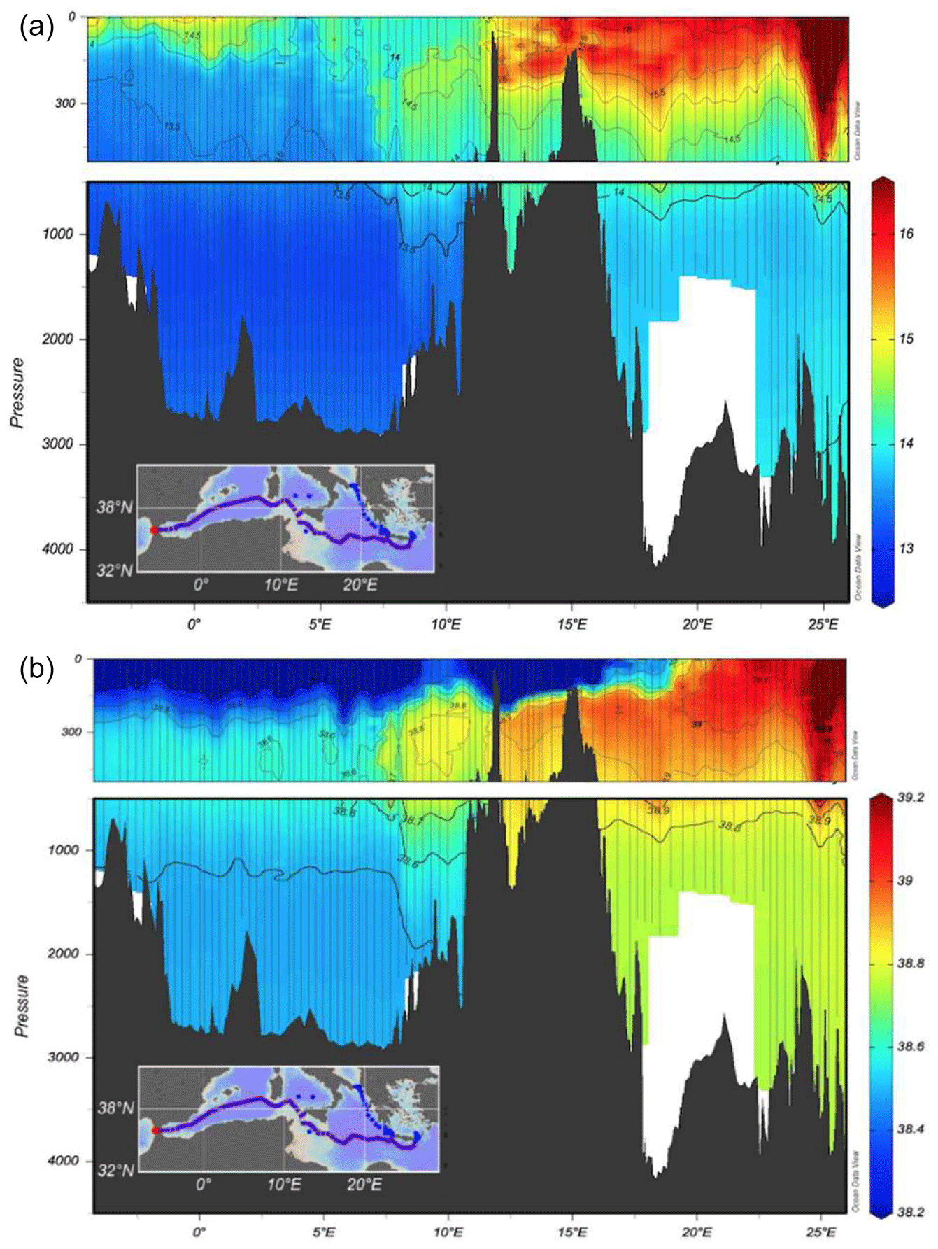
Figure 2West–east temperature (a) and salinity (b) sections through the Mediterranean Sea.

Figure 3The uCTD salinity transect; the location is shown in the inset.
3.14 LISST-DEEP
The LISST-Deep instrument obtains in situ measurements of particle size distribution, optical transmission, and the optical volume scattering function (VSF) at depths down to 3000 m. It is manufactured by Sequoia Inc. and owned by the Hellenic Centre for Marine Research (HCMR), Greece.
Using a red 670 nm diode laser and a custom silicon detector, small-angle scattering from suspended particles is sensed at 32 specific log-spaced angle ranges. This primary measurement is post-processed to obtain sediment size distribution, volume concentration, optical transmission, and volume scattering function. The LISST-Deep s/n 4004 is categorized as a type B instrument, which means that the range of particles it measures ranges from 1.25 to 250 µm. The LISST-Deep must be powered externally at all times. This is typically achieved by connecting it to a rosette, getting power from the main CTD unit.
Parameters measured during the cruise were as follows:
-
particle size distribution from 1.25–250 or 2.5–500 µm;
-
depth (3000 m max depth at 0.8 m resolution);
-
optical transmission at 0.1 % resolution;
-
beam attenuation coefficient at 0.1 m−1 resolution;
-
volume concentration at 0.1 µL L−1 resolution;
-
volume scattering function (VSF).
The measurement of these parameters provided important information about the number, size and quality (phytoplankton, sediment, etc.) of the suspended matter in the water column. Further information for the determination of water masses was provided by the estimation of the intrinsic optical properties. Finally, for the first ∼100 m we estimated the color of the sea and compared this estimation with satellite images, providing valuable information for the calibration of satellite algorithms.
For the cruise MSM72 the sampling of these optical estimates is in itself an important achievement because, for the first time, LISST-DEEP was used to record data in a transect over the full length of the Mediterranean Sea. Furthermore, the estimation of these parameters, combined with Particulate Organic Carbon - Particulate Organic Nitrogen (POC-PON) estimation and other physical and chemical parameters, improves the study of the dynamics of the Mediterranean Sea.
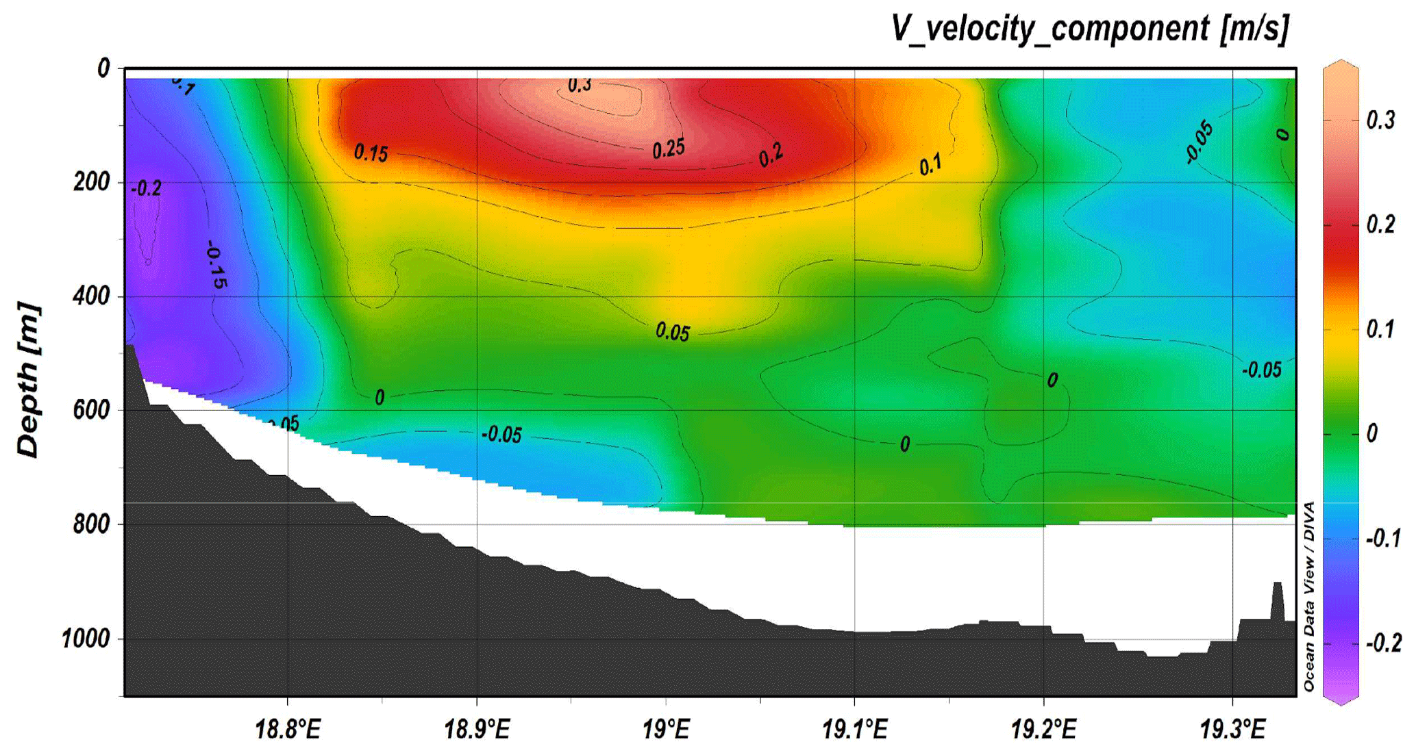
Figure 4Transect across the Otranto Strait from ADCP 38, positive numbers correspond to northward currents.
In general, the use of LISST-DEEP during the cruise follows the standard methods provided by Sequoia Inc. but with one important difference. For the estimation of the above parameters the use of a background file is required for normalization purposes. This file is normally produced in laboratory conditions with MilliQ 2 filtered water. However, experience until now has proved that the use of this background file leads us to an overestimation of the parameters and especially of the beam attenuation coefficient, especially in the eastern Mediterranean Sea (which is characterized as ultra-oligotrophic). Therefore, during this cruise we used a sampled in situ background file chosen as the minimum of the sum of the digital counts in the 32 rings and where the LaserPower to LaserReference (Lp/Lr) ratio is at a maximum.
The main problem, which we faced, was the frequent change of the CTD main unit and the different cables that we had to use for the instrument connection to the CTD. Fortunately, with the most valuable help of the cruise technician, we managed to deploy the LISST-DEEP as much as possible. Additionally, the maximum depth limitation of the instrument (3000 m) forced us to remove it in deep casts, achieving a total of 54 stations.
Data are published at the information systems PANGAEA and CCHDO: https://doi.org/10.1594/PANGAEA.905902 (CTD, Hainbucher et al., 2019); https://doi.org/10.1594/PANGAEA.913512 (UCTD, Hainbucher, 2020a); https://doi.org/10.1594/PANGAEA.913608 (ADCP, Hainbucher, 2020b); https://doi.org/10.1594/PANGAEA.913505 (lADCP, Hainbucher, 2020c); https://doi.org/10.1594/PANGAEA.905887 (chemical data, Tanhua et al., 2019); https://doi.org/10.25921/z7en-hn85 (pCO2, Tanhua et al., 2020); https://cchdo.ucsd.edu/cruise/06M220180 (last access: 10 November 2020) (additional CTD and chemical data).
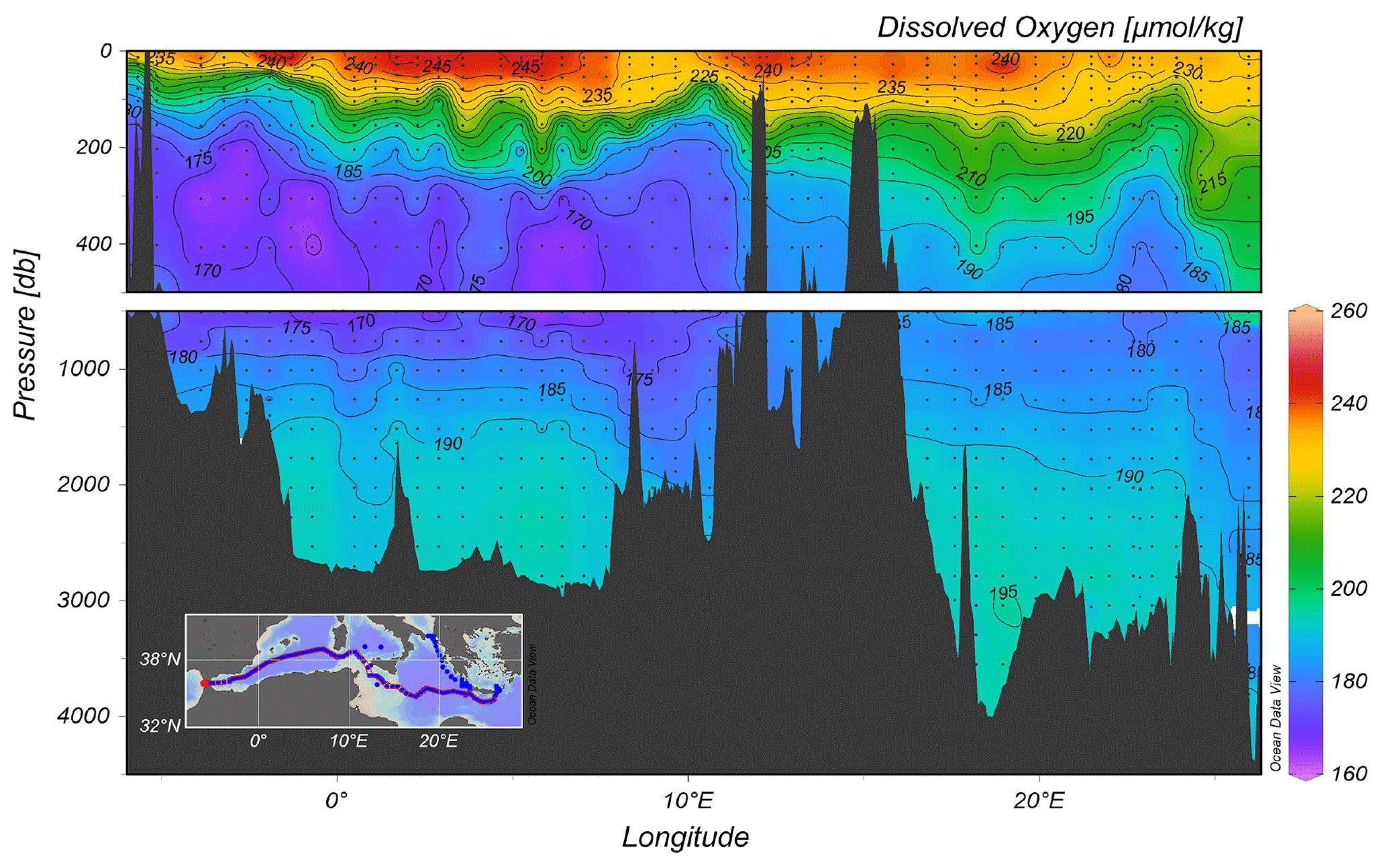
Figure 5Distribution of dissolved oxygen along the trans-Mediterranean section.
This discussion and conclusion will focus on the quality of the data of MSM72 cruise. We will concentrate here on the basic physical and biogeochemical parameters as selected examples to show the relevance of the sampled data and in order for us to be able to answer the questions on the scale and variability of the circulation and biogeochemical cycle in the Mediterranean Sea (see the Introduction).
5.1 Physical parameters
The west–east section (Fig. 2) is a typical example for the distribution of temperature and salinity in the Mediterranean Sea showing the different heat and salt content between the western and eastern basin. A clear intrusion of the salty Levantine Intermediate Water (LIW) from east to west in the first 500 m is depicted, while the low-salinity Atlantic Water (AW) protrudes eastwards creating a front at about 20–22∘ E.
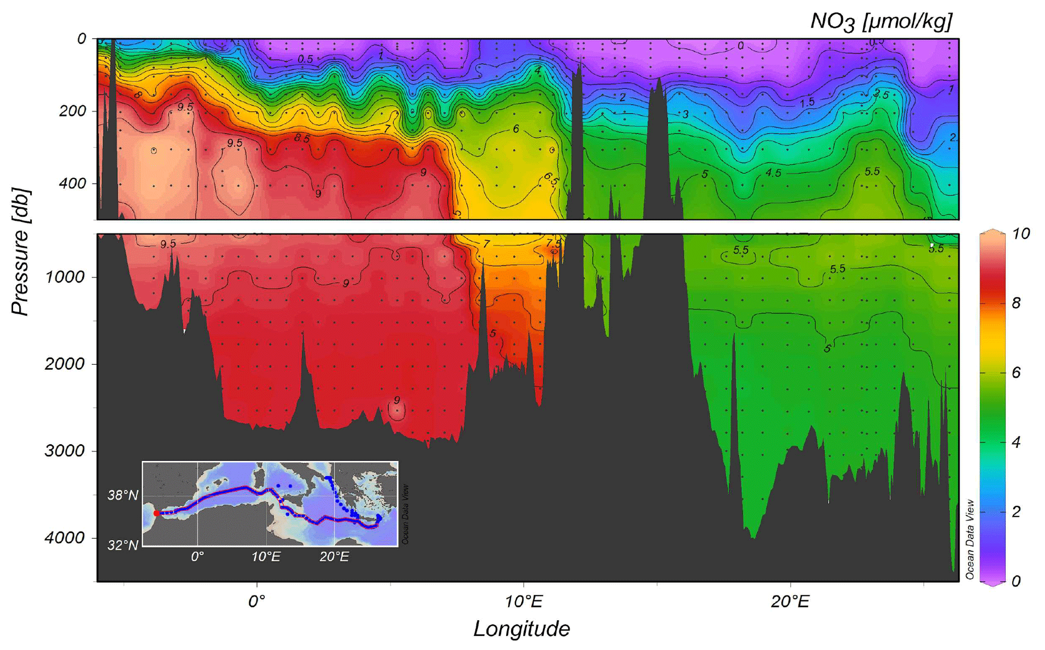
Figure 6Distribution of nitrate along the trans-Mediterranean section.

Figure 7DOC vertical distribution along the trans-Mediterranean section.
The underway CTD data are a valuable addition to the classical CTD data. They enhance the resolution of data in the horizontal scale and give insight into eddy activity. Although the data do not reach to the bottom, the vertical resolution with about 1000 m is useful to characterize scales relevant for the LIW transport.
The uCTD stations along the easternmost part of the northward transit in the Ionian Sea are taken every 5 nm on average. Larger gaps in the line were essentially caused by the deployment of CTD stations. The uCTD salinity distribution of Fig. 3 shows that the Pelops gyre is well resolved.
Considering the route of the ship during the cruise, it was possible to identify different ADCP transects that correspond to areas with the most important water mass dynamics. In particular, the most important sections were gyre activity in the area west of Crete and south of the Peloponnese; the west Cretan, Otranto (Fig. 4), and Sicilian straits; the eastern boundary of the Ionian Sea; and the west–east Mediterranean transect. The north–south current component (Fig. 4) in the Otranto Strait clearly shows the outflow of the Adriatic Deep Water (AdDW) along the western part, while in the upper and intermediate layer of the central part the inflow of the Levantine Intermediate Water (LIW) proceeds.
5.2 Biogeochemical parameters
The vertical distribution of dissolved oxygen along a section from the Cretan Sea to Gibraltar, including part of the Cretan Passage and the southern Ionian Sea, is shown in Fig. 5. This section shows the Oxygen Minimum Layer (<180 µmoles kg−1), which occupies the layer 500–1500 m. Increased oxygen towards the bottom indicate the ventilation of deep water in the Mediterranean. The western part of the Ionian Sea appears to be better oxygenated than the eastern part due to the spreading of newly ventilated dense water from the Adriatic Sea via the Otranto Strait, a feature that is observed in the transient tracer section as well.
Figure 6 illustrates the distribution of nitrate along the quasi-zonal section. Interesting features include the maximum nutrient layer in the range of depth of 500–1500 m, which is co-located to the minimum of transient tracers. The deepest layer shows an homogeneous distribution of nutrients and the nutrient impoverished upper layer is not yet completely depleted of nutrients, likely due to mesoscale dynamics (as is the case, for example, south of Crete).
The DOC data collected during the MSM72 cruise represents an unique opportunity to (i) investigate the long-term variation in DOC distribution in intermediate and deep waters on a basin scale, (ii) quantify the role of DOC in C export and sequestration in the Mediterranean Sea, (iii) estimate DOC mineralization rates, and (iv) assess the functioning of microbial loop in the different areas of the Mediterranean Sea.
DOC concentrations range between 34 and 80 µM (Fig. 7). The highest values (>50 µM) were observed in the upper 200 m, with a marked increase moving eastward. The lowest concentrations (<40 µM) are between 1000 and 2000 m; in the bottom waters a slight increase in DOC can be observed. This feature, already reported for the Mediterranean Sea, can be explained by the export of the DOC accumulated in the surface layer by deep water formation (Santinelli, 2015, and references therein). The high stratification, occurring in the easternmost stations, makes DOC accumulation there more visible. A different functioning of the microbial loop has been reported for the western and eastern Mediterranean Sea and these data support that DOC dynamics in the surface layer of the two sub-basins is different.
DH and TT designed the experiment and were responsible for the cruise, and DH was chief scientist of the cruise. All authors either took part in the cruise and/or were involved in the data processing. All authors discussed and approved the manuscript.
The authors declare that they have no conflict of interest.
We thank Captain Björn Maaß, his officers and the crew of R/V Maria S. Merian for their support of our scientific program and their unending competent and friendly help.
The financial support for the cruise was provided by the project of the Deutsche Forschungsgemeinschaft (grant no. U4600DFG040204). We gratefully acknowledge their support.
The CO2 team was funded by an internal IEO grant MEDSHIP18. Abed El Rahman Hassoun Hassoun was funded by a POGO grant. The OGS team was funded by an internal grant.
This research has been supported by the Deutsche Forschungsgemeinschaft (grant no. U4600DFG040204).
This paper was edited by Giuseppe M. R. Manzella and reviewed by two anonymous referees.
Bullister, J. L. and Weiss, R. F.: Determination of CCl3F and CCl2F2 in seawater and air, Deep-Sea Res., 35, 839–853, 1988.
Byrne, R. H. and Yao, W.: Procedures for measurement of carbonate ion concentrations in seawater by direct espectrophotometric observations of Pb (II) complexation, Mar. Chem., 112, 128–135, 2008.
Carlson, C. A. and Hansell, D. A.: Biogeochemistry of Marine Dissolved Organic Matter, 2nd edn., Elsevier Inc., 66–126, https://doi.org/10.1016/C2012-0-02714-7, 2015.
Casciotti, K. L., Sigman, D. M., Galanter Hastings, M., Böhlke, J. K., and Hilkert, A.: Measurement of the oxygen isotopic composition of nitrate in seawater and freshwater using the denitrifier method, Anal. Chem., 74, 4905–4912, 2002.
Clayton, T. D. and Byrne, R. H.: Spectrophotometric seawater pH measurements: total hydrogen ion concentration scale concentration scale calibration of m-cresol purple and at-sea results, Deep-Sea Res. Pt. I, 40, 2115–2129, 1993.
Gerke, L.: pCO2 in the Mediterranean Sea during the cruise MSM72. Master thesis, Department of Chemistry, Christian-Albrechts-University, Kiel, 2020.
Gonnelli, M., Galletti, Y., Marchetti, E., Mercadante, L., Brogi, S. R., Ribotti, A., Sorgente, R., Vestri, S., and Santinelli, C.: Dissolved organic matter dynamics in surface waters affected by oil spill pollution: Results from the serious game exercise, Deep-Sea Res. Pt. II, 133, 88–99, 2016.
Granger, J. and Sigman, D. M.: Removal of nitrite with sulfamic acid for nitrate N and O isotope analysis with the denitrifier method, Rapid Commun. Mass Spectrom., 23, 3753–3762, https://doi.org/10.1002/rcm.4307, 2009.
Häder, D.-P. and Sinha, R. P.: Solar ultraviolet radiation-induced DNA damage in aquatic organisms: potential environmental impact, ScienceDirect, https://doi.org/10.1016/j.mrfmmm.2004.11.017, 2005.
Hainbucher, D.: Underway CTD data during MARIA S. MERIAN cruise MSM72, PANGAEA, https://doi.org/10.1594/PANGAEA.913512, 2020a.
Hainbucher, D.: ADCP current measurements (38 and 75 kHz) during MARIA S. MERIAN cruise MSM72, PANGAEA, https://doi.org/10.1594/PANGAEA.913608, 2020b.
Hainbucher, D.: Lowered ADCP data during MARIA S. MERIAN cruise MSM72, PANGAEA, https://doi.org/10.1594/PANGAEA.913505, 2020c.
Hainbucher, D., Álvarez, M., Astray, B., Bachi, G., Cardin, V., Celentano, P., Chaikakis, S., Chaves Montero, M. M., Civitarese, G., El Rahman Hassoun, H., Fajar, N. M., Fripiat, F., Gerke, L., Gogou, A., Guallart, F., Gülk, B., Lange, N., Rochner, A., Santinelli, C., Schroeder, K., Steinhoff, Tanhua, T., Urbini, L., Velaoras, D., Wolf, F., and Welsch, A.: Variability and Trends in Physical and Biogeochemical Parameters of the Mediterranean Sea, available at: http://epic.awi.de/47567/2/msm71-74-expeditionsheft.pdf (last access: 10 November 2020), 2018.
Hainbucher, D., Cardin, V., Velaoras, D., and Montero, M. F.: Physical oceanography during MARIA S. MERIAN cruise MSM72, PANGAEA, https://doi.org/10.1594/PANGAEA.905902, 2019.
Hansell, D. A., Carlson, C. A., Pepeta, D. L., and Schlitzer, R.: Dissolved Organic Matter in the Ocean: A controversy stimulates new insights, Oceanography, 22, 202–211, 2009.
Hansen, H. P. and Koroleff, E.: Determination of nutrients, in: Methods of seawater analysis, edited by: Grasshoff, K., Kremling, K., and Ehrhardt, M., Wiley VCH, Weinheim, 159–228, 1999.
Herndl, G. J., Müller-Niklas, G., and Frick, J.: Major role of ultraviolet-B in controlling bacterio plankton growth in the surface layer of the ocean, Nature, 361, 717–719, 1993.
Johnson, K. M., Wills, K. D., Butler, D. B., Johnson, W. K., and Wong, C. S.: Coulometric total carbon dioxide analysis for marine studies: maximizing the performance of an automated gas extraction system and coulometric detector, Marine Chem., 44, 167–187, 1993.
Langdon, C.: Determination of dissolved oxygen in seawater by Winkler titration using the amperometric technique, IOCCP Report No. 14, ICPO publication series N 134, 2010.
Li, P. and Tanhua, T.: Medusa-Aqua system: simultaneous measurement and evaluation of novel potential halogenated transient tracers HCFCs, HFCs and PFCs in the ocean, Ocean Sci. Discuss., https://doi.org/10.5194/os-2019-101, in review, 2019.
Li, P. and Tanhua, T.: Recent Changes in Deep Ventilation of the Mediterranean Sea; Evidence from Long-Term Transient Tracer Observations, Front. Marine Sci., 7, 1–23, https://doi.org/10.3389/fmars.2020.00594, 2020.
Malanotte-Rizzoli, P., Artale, V., Borzelli-Eusebi, G. L., Brenner, S., Crise, A., Gacic, M., Kress, N., Marullo, S., Ribera d'Alcalà, M., Sofianos, S., Tanhua, T., Theocharis, A., Alvarez, M., Ashkenazy, Y., Bergamasco, A., Cardin, V., Carniel, S., Civitarese, G., D'Ortenzio, F., Font, J., Garcia-Ladona, E., Garcia-Lafuente, J. M., Gogou, A., Gregoire, M., Hainbucher, D., Kontoyannis, H., Kovacevic, V., Kraskapoulou, E., Kroskos, G., Incarbona, A., Mazzocchi, M. G., Orlic, M., Ozsoy, E., Pascual, A., Poulain, P.-M., Roether, W., Rubino, A., Schroeder, K., Siokou-Frangou, J., Souvermezoglou, E., Sprovieri, M., Tintoré, J., and Triantafyllou, G.: Physical forcing and physical/biochemical variability of the Mediterranean Sea: a review of unresolved issues and directions for future research, Ocean Sci., 10, 281–322, https://doi.org/10.5194/os-10-281-2014, 2014.
Margolin, A. R., Gonnelli, M., Hansel, D. A., and Santinelli, C.: Black Sea dissolved organic matter dynamics: Insights from optical analyses, Limnol. Oceanogr., 63, 1425–1443, https://doi.org/10.1002/lno.10791, 2018.
Mintrop, L., Pérez, F. F., González-Dávila, M., Körtzinger, A., and Santana-Casiano, J. M.: Alkalinity determination by potentiometry-intercalibration using three different methods, Ciencias Marinas, 26, 23–37, 2000.
Nelson, N. B. and Siegel, D. A.: The global distribution and dynamics of chromophoric dissolved organic matter, Annu. Rev. Mar. Sci., 5, 447–476, 2013.
Patsavas, M. C., Byrne, R. B., Yang, B., Easley, R. A., Wanninkhof, R., and Liu, X.: Procedures for direct spectrophotometric determination of carbonate ion concentrations: Measurements in US Gulf of Mexico and East Coast waters, Mar. Chem., 168, 80–85, 2015.
Pérez, F. F. and Fraga, F.: A precise and rapid analytical procedure for alkalinity determination, Marine Chem., 21, 169–182, 1987.
Pérez, F. F., Ríos, A. F., Rellán, T., and Álvarez, M.: Improvements in a fast potentiometric seawater alkalinity determination, Ciencias Marinas, 26, 463–478, 2000.
Retelletti Brogi, S., Gonelli, M., Vestri, S., and Santinelli, C.: Biophysical processes affecting DOM dynamics at the Arno river mouth (Tyrrhenian Sea), Biophys. Chem., 197, 1–9, 2015.
Roether, W., Klein, B., and Hainbucher, D.: The Eastern Mediterranean Transient: Evidence for Similar Events Previously?, in: The Mediterranean Sea: Temporal Variability and Spatial Patterns, edited by: Borzelli, G. L. E., AGU monographs, https://doi.org/10.1002/9781118847572.ch6, 2013.
Santinelli, C.: DOC in the Mediterranean Sea, in: Biogeochemistry of Marine Dissolved Organic Matter, 2nd edn., 579–08, 2015.
Santinelli, C., Hansell, D. A., and Ribera d'Alcala, M.: Influence of stratification on marine dissolved organic carbon (DOC) dynamics: The Mediterranean Sea case, Prog. Oceanogr., 119, 68–77, 2013.
Santinelli, C., Follet C., Retelletti Brogi, S., Xu, L., and Repeta, D.: Carbon isotope measurements reveal unexpected cycling of dissolved organic matter in the deep Mediterranean Sea, Marine Chem., 177, 267–277, 2015.
Schneider, A., Tanhua, T., Körtzinger, A., and Wallace, D. W. R.: High anthropogenic carbon content in the eastern Mediterranean, J. Geophys. Res., 115, C12050, https://doi.org/10.1029/2010JC006171, 2010.
Schroeder, K., Gasparini, G. P., Tangherlini, M., and Astraldi, M.: Deep and intermediate water in the western Mediterranean under the influence of the Eastern Mediterranean Transient, Geophys. Res. Lett., 33, L21607, https://doi.org/10.1029/2006GL027121, 2006.
Schroeder, K., Ribotti, A., Borghini, M., Sorgente, R., Perilli, A., and Gasparini, G. P.: An extensive western Mediterranean deep water renewal between 2004 and 2006, Geophys. Res. Lett., 35, https://doi.org/10.1029/2008GL035146, 2008.
Sigman, D. M., Casciotti, K. L., Andreani, M., Barford, C., Galanter, M., and Böhlke, J. K.: A bacterial method for the nitrogen isotopic analysis of nitrate in seawater and freshwater, Anal. Chem., 73, 4145–4153, 2001.
Stedmon, C. A. and Nelson, N. B.: The optical properties of DOM in the Ocean, in: Biogeochemistry of Marine Dissolved Organic Matter, 2nd edn., Elsevier, edited by: Hansell, D. A. and Carlson, C. A., chapter 10, 481–508, https://doi.org/10.1016/B978-0-12-405940-5.00010-8, 2015.
Tanhua, T. and Steinhoff, T.: Surface underway measurements of partial pressure of carbon dioxide (pCO2), salinity, temperature and other associated parameters during the R/V MARIA S. MERIAN cruise (EXPOCODE 06M220180302) in Mediterranean Sea from 2018-03-02 to 2018-04-03 (NCEI Accession 0208442), NOAA National Centers for Environmental Information, Dataset, https://doi.org/10.25921/z7en-hn85, 2020.
Tanhua, T., Hainbucher, D., Schroeder, K., Cardin, V., Álvarez, M., and Civitarese, G.: The Mediterranean Sea system: a review and an introduction to the special issue, Ocean Sci., 9, 789–803, https://doi.org/10.5194/os-9-789-2013, 2013.
Tanhua, T., Álvarez, M., and Civitarese, G.: Hydrochemistry of water bottles during MARIA S. MERIAN cruise MSM72, PANGAEA, https://doi.org/10.1594/PANGAEA.905887, 2019.
Turnherr, A. M.: How to Process LADCP Data with the LDEO Software (Versions IX.7–IX.10). The “go-ship” manual for LADCP data acquisition, available at: ftp://ftp.ldeo.columbia.edu/pub/LADCP/UserManuals (last access: 10 November 2020), 2014.
Ullmann, D. S. and Hebert, D.: Processing of Underway CTD data, AMS, https://doi.org/10.1175/JTECH-D-13-00200.1, 2014.
Weigand, M. A., Foriel, J., Barnett, B., Oleynik, S., and Sigman, D. M.: Updates to instrumentation and protocols for isotopic analysis of nitrate by the denitrifier method, Rapid Commun. Mass Spectrom., 30, 1365–1383, 2016.