the Creative Commons Attribution 4.0 License.
the Creative Commons Attribution 4.0 License.
 | 31 Oct 2020
The Global Space-based Stratospheric Aerosol Climatology (version 2.0): 1979–2018
Mahesh Kovilakam
Larry W. Thomason
Nicholas Ernest
Landon Rieger
Adam Bourassa
Luis Millán
A robust stratospheric aerosol climate data record enables the depiction of the radiative forcing of this highly variable component of climate. In addition to the radiative forcing, stratospheric aerosol also plays a key role in the chemical processes leading to ozone depletion. Therefore, stratospheric aerosol is one of the crucial parameters in understanding climate change in the past and potential changes in the future. As a part of Stratospheric-tropospheric Processes and their Role in Climate (SPARC) Stratospheric Sulfur and its Role in Climate (SSiRC) activity, the Global Space-based Stratospheric Aerosol Climatology (GloSSAC) was created (Thomason et al., 2018) to support the World Climate Research Programme's (WCRP) Coupled Model Intercomparison Project Phase 6 (CMIP6) (Eyring et al., 2016). This data set is a follow-on to one created as a part of SPARC's Assessment of Stratospheric Aerosol Properties (ASAP) activity (SPARC, 2006) and a data created for the Chemistry-Climate Model Initiative (CCMI) in 2012 (Eyring and Lamarque, 2012). Herein, we discuss changes to the original release version including those as a part of v1.1 that was released in September 2018 that primarily corrects an error in the conversion of Cryogenic Limb Array Etalon Spectrometer (CLAES) data to Stratospheric Aerosol and Gas Experiment (SAGE) II wavelengths, as well as the new release, v2.0. Version 2.0 is focused on improving the post-SAGE II era (after 2005) with the goal of mitigating elevated aerosol extinction in the lower stratosphere at mid- and high latitudes noted in v1.0 as noted in Thomason et al. (2018). Changes include the use of version 7.0 of the Optical Spectrograph and InfraRed Imaging System (OSIRIS), the recently released Cloud-Aerosol Lidar and Infrared Pathfinder Satellite Observation (CALIPSO) lidar Level 3 stratospheric aerosol profile monthly product and the new addition of SAGE III/ISS. Here, we use an observed relationship between (i) OSIRIS extinction at 750 nm and (ii) SAGE II and SAGE III/ISS extinction at 525 nm to derive an altitude–latitude-based monthly climatology of Ångström exponent to compute OSIRIS extinction at 525 nm, resulting in a better agreement between OSIRIS and SAGE measurements. We employ a similar approach to convert OSIRIS 750 nm extinction to 1020 nm extinction for the post-SAGE II period. Additionally, we incorporate the recently released standard CALIPSO stratospheric aerosol profile monthly product into GloSSAC with an improved conversion technique of the 532 nm backscatter coefficient to extinction using an observed relationship between OSIRIS 525 nm extinction and CALIPSO 532 nm backscatter. SAGE III/ISS data are also incorporated in GloSSAC to extend the climatology to the present and to test the approach used to correct OSIRIS/CALIPSO data. The GloSSAC v2.0 netCDF file is accessible at https://doi.org/10.5067/glossac-l3-v2.0 (Thomason, 2020).
- Article
(13972 KB) - Full-text XML
-
Supplement
(155 KB) - BibTeX
- EndNote


Stratospheric aerosols play a key role in determining the chemical (e.g., Hofmann and Solomon, 1989; Fahey et al., 1993; Solomon et al., 1996) and radiative (e.g., Minnis et al., 1993; Ridley et al., 2014) balance of the atmosphere. Variations in the stratospheric aerosol levels due to volcanic activity can impact climate on the magnitudes from subtle surface temperatures changes (e.g., Solomon et al., 2011) to the more profound surface cooling (e.g., Hansen et al., 1992; Robock and Mao, 1995; Robock, 2000) and associated precipitation changes (e.g., Haywood et al., 2013; Iles et al., 2013).
The impact of volcanic eruptions is often studied using global climate models (GCMs). Some of these modeling studies (e.g., Stenchikov et al., 2006; Berdahl and Robock, 2013; Fyfe et al., 2013) rely on observational data to represent stratospheric aerosols while others (e.g., Aquila et al., 2013; Mills et al., 2016; Timmreck et al., 2018) interactively model stratospheric aerosol variations. A robust stratospheric aerosol climatology can play a key role in the success of both approaches to modeling the effects of stratospheric aerosol either as a direct input to GCMs or as an observational data set with which to verify the performance of an interactive aerosol scheme (e.g., Aquila et al., 2013; Mills et al., 2016). The GloSSAC data set has also been used in an observational study (Stocker et al., 2019) to quantify the temperature footprint of 21st century eruptions that enables us to better quantify temperature trends related to anthropogenic forcing. As a part of SPARC's SSiRC activity, GloSSAC was created (Thomason et al., 2018) to support, among other endeavors, the WCRP's CMIP6 project (Eyring et al., 2016; Zanchettin et al., 2016). This data set spans from 1979 to 2016 and is a follow-on to one created as a part of SPARC's Assessment of Stratospheric Aerosol Properties (ASAP) activity (SPARC, 2006). Herein, we report on the development of GloSSAC version 2.0 data that extends the data set through 2018. While data sources are mostly unchanged from earlier versions, there are significant improvements in the use of OSIRIS and CALIPSO data with inclusion of SAGE III/ISS data for the first time. As a result, a major version change is warranted and users should use this version even for periods prior to the end of v1.1 (December 2016).
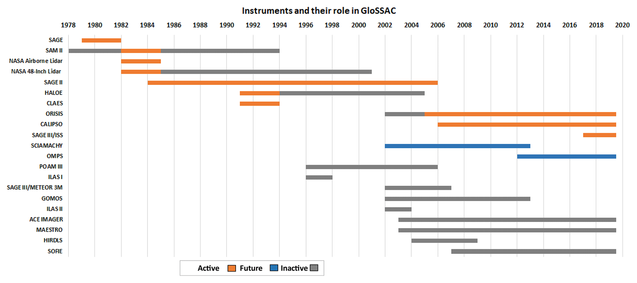
Figure 1Space-based measurements of stratospheric aerosol extinction coefficient data used in GloSSAC.
Figure 1 depicts the measurements that are currently used for constructing GloSSAC data. While Thomason et al. (2018) discusses the measurements that have been used in the GloSSAC v1.0 data set in detail, some of the main features of entire GloSSAC v2.0 data set including various space-based measurements, their limitations and some challenges are worth mentioning here. We divide the entire data set into three periods based on the measurements used. The first period is the pre-SAGE II period (January 1979–September 1984), followed by the SAGE II period (October 1984–August 2005), post-SAGE II period (September 2005–May 2017) and SAGE III/ISS period (June 2017–present). Pre-SAGE II period data mostly consist of data from solar occultation measurements such as SAM II, SAGE and some surface-based lidar measurements (Thomason et al., 2018). For the SAGE II period, the measurements are dominated by solar occultation measurements that provide multiwavelength measurements for size information. For the post-SAGE II era, we are limited to single-wavelength measurements from OSIRIS and/or CALIPSO. While OSIRIS and CALIPSO continue to make daily global measurements with a less direct measurement of the aerosol extinction coefficient that requires further assumption of particle size, additional direct measurements of the aerosol extinction coefficient from SAGE III/ISS that provides a roughly monthly coverage of multiwavelength measurements since June 2017 are now available.
We now use OSIRIS version 7.0 rather than the previous release version 5.07. OSIRIS (2001 to present) remains a key component of the GloSSAC data as it is the only data set that spans both the SAGE II period (1984–2005) and the start of the SAGE III/ISS mission in 2017. In version 5.07, aerosol extinction at 750 nm was retrieved at approximately 2 km resolution using a multiplicative relaxation technique (Bourassa et al., 2012). OSIRIS version 7.0 data (Rieger et al., 2019) uses a multiwavelength retrieval that improves the accuracy of the extinction product by reducing sensitivity to the unknown particle size distribution in the inversion. With these changes, the retrieved extinction coefficient at 750 nm is in better agreement with observations by SAGE II and SAGE III/ISS than the version used in GloSSAC v1.0 (v5.07). A detailed description of the retrieval process and comparisons to SAGE II and SAGE III/ISS are available in Rieger et al. (2019). It should be noted that while the OSIRIS mission continues, data for 2018 is not available at the time the data record was developed and thus not included in the GloSSAC data set.
We continue to make use of CALIPSO's Cloud-Aerosol Lidar with Orthogonal Polarization (CALIOP) aerosol backscatter coefficient measurements. The CALIPSO mission (Winker et al., 2009) has been providing cloud and aerosol profiles since 2006. CALIOP data were used in GloSSAC v1.0 during the post-SAGE II era, critically in regions and time periods where OSIRIS data are not available. For GloSSAC v1.0, we used the CALIOP version 4.0 level 1 aerosol data product at 532 nm and identified and removed observations that suggested the presence of cloud using the depolarization measurement. The remaining data were compiled into the spatial temporal resolution used in GloSSAC (monthly, 5∘ latitude bins and 0.5 km altitude bins). Since the release of GloSSAC v1.0, the CALIPSO team has released a standard stratospheric aerosol extinction and backscatter products (Kar et al., 2019) in a spatial/temporal resolution compatible with GloSSAC. This data product is now used rather than the level 1 data. While we use the standard CALIPSO stratospheric aerosol product, enhanced levels of aerosol extinction in the lower stratosphere are consistently noted in the entire data set after comparing against OSIRIS and SAGE III/ISS. We therefore decided to use a conformance process which is described below that helps reduce the bias in the lower stratosphere and also at higher latitudes.
New to GloSSAC, we now use version 5.1 data from the latest series of Stratospheric Aerosol and Gas Experiment on International space station (SAGE III/ISS) satellite measurements. Like SAGE II, SAGE III/ISS uses the solar occultation technique (McCormick et al., 1979) to make near-global measurements of stratospheric aerosol, ozone, water vapor and nitrogen dioxide with a vertical resolution of 1 km on a roughly monthly timescale. Aerosol extinction coefficients at nine wavelengths are provided including at the GloSSAC standard wavelengths near 525 and 1020 nm. SAGE III/ISS data are available from June 2017, and we incorporate the data into GloSSAC from that time forward as the primary data set similar to the way in which SAGE and SAGE II are used earlier in the data record.
For individual instruments, we have expanded the practice of including data in the original parameter and wavelength as possible (e.g., OSIRIS extinction at 750 nm, and CALIOP backscatter coefficient) in the GloSSAC spatial temporal resolution and now include most data sets as components of the GloSSAC data set. The point of origin of each individual data set is clearly denoted for all data points in the now 40-year record at the primary 525 and 1020 nm wavelengths. As with v1.0, we recommend using original, unconformed and uninterpolated data for comparison purposes. Conformance follows the basic paradigm of v1.0 but has changed in some instances to reflect better understanding of instrumental differences (Thomason et al., 2018). SAGE II version 7.0 continues to act as the standard throughout the data set. As a result, similar to GloSSAC v1.0, data from other platforms and sometimes made of different aerosol properties and/or at different wavelengths are made, on average, to match or “conform” with SAGE II at 525 and 1020 nm. This is mostly done using simple linear scaling factors rather than retaining offsets that may be created by switching from one data source to another. For instance in v1.0, the conversion factor used for the 532 nm backscatter coefficient to the 525 nm aerosol extinction coefficient (53 sr) was selected to minimize the overall difference between SAGE II and CALIOP backscatter data (Thomason et al., 2018). An exception to this process was the higher-than-expected extinction in the lower stratosphere in mid- and high latitudes during the CALIOP/OSIRIS era based on observations at similar overall aerosol levels during the SAGE II period. Both GloSSAC v1.0 and v1.1 retained these offsets in extinction as, at the time, it was not clear if the difference was due to real geophysical variability possibly driven by volcanic activity or due to deficiencies in conversion process or in the source data themselves. A goal of this release was to understand and, as necessary, mitigate this discrepancy (Thomason et al., 2018). While the changes in the both CALIOP and OSIRIS source data sets have reduced the apparent anomaly in extinction inferred for this period, both data sets, adjusted using the conformance approaches used in v1.0, continue to suggest higher levels of the aerosol extinction coefficient in the lower stratosphere than observations by SAGE II would suggest. At the same time, very similar discrepancies were noted between OSIRIS and CALIOP data and SAGE III/ISS observations some 12 years later. Given these facts, we are now confident that these differences are due to measurement/conformance deficiencies, and we have developed new techniques to bring these data sets into greater conformity with SAGE II; they are discussed below.
Additional changes to this GloSSAC version relative to the v1.0 as described in Thomason et al. (2018) include all changes made in the interim version 1.1. The changes made to interim version 1.1 are described below in Sect. 2.1. Within v2.0, a key data set (McCormick et al., 1979) used in the SAGE/SAGE II gap period (1982–1984) has been updated. We have expanded the GloSSAC v2.0 netCDF to include stratospheric aerosol optical depth at the primary reporting wavelengths of 525 and 1020 nm, and we now retain the native measurements for all instrument data sets (e.g., CALIOP backscatter coefficient at 532 nm) as well as values after conversion to 525 and/or 1020 nm. We also now include reported measurement uncertainty and zonal variability where available at both the native measurement form and at the GloSSAC extinction wavelengths. The updated file resides at NASA's Atmospheric Sciences Data Center and has a unique https://doi.org/10.5067/GLOSSAC-L3-V2.0.
2.1 Changes prior to the end SAGE II period
2.1.1 Updates to the SAGE II era (October 1984–August 2005)
Since the release of GloSSAC v1.0, an interim version was released that corrected a coding error in the initial implementation of the conversion of CLAES infrared aerosol extinction coefficient data to the SAGE II and primary GloSSAC reporting wavelength at 1020 nm. The primary impact was a substantial exaggeration, sometimes exceeding a factor of 2, in the peak aerosol extinction associated with the Pinatubo eruption in the tropics in the several months following the eruption in June 1991. CLAES data become available in October 1991 but are used in combination with a ground-based lidar product to estimate the aerosol levels from July to September 1991 and are used standalone for a decreasing span of altitude and latitude until the end of its mission in April 1993 (Thomason et al., 2018; SPARC, 2006). The use of CLAES (Massie et al., 1996) and Halogen Occultation Experiment (HALOE) (Thomason, 2012) data in GloSSAC version 1.1 was also decreased by only employing it to fill latitude/temporal bins in which SAGE II data existed but did not extend as low as the tropopause. This significantly reduced the impact of both CLAES and HALOE in the data set but made spatial and temporal sampling in this period more consistent the sampling throughout SAGE II mission. These changes are continued into v2.0. Some additional quality control (QC) was performed that caught a few defects missed in v1.0.
Compared to the important change requiring the release of version 1.1, only relatively minor additional changes to the SAGE II and pre-SAGE II portions of the data set are included in v2.0. The changes to the SAGE II era within GloSSAC include improved outlier filtering for the SAGE II aerosol extinction coefficient data. In this case, we eliminate as outliers any data in a GloSSAC bin that exceeds 3.5 median absolute deviations from the median value of all observations within a GloSSAC bin. This filtering has a minimal impact on the results for 452, 525 and 1020 nm but substantially reduces noise in the data at 386 nm and reduces the need for manual QC repairs of that data set. Users should continue to use caution using the SAGE II 386 nm aerosol extinction coefficient data as a low bias is evident in these data in the lower and upper stratosphere and at all altitudes as aerosol extinction coefficient magnitudes approach background levels (Thomason et al., 2008, 2018). Where aerosol extinction is only available at 1020 nm, the extinction coefficient data sets at 452 and 386 nm are now filled using the same mechanism to fill missing data at 525 nm so that all four wavelength arrays are complete above the tropopause throughout the SAGE II era, as is described in Thomason et al. (2018).
In addition, with the apparent success of filling the high latitudes using the equivalent latitude/latitude mechanism developed based on Manney et al. (2007) for v1.0 (Thomason et al., 2008), we have reduced the role of simple linear interpolation at high latitudes and allow the new equivalent latitude/latitude mechanism to fill more of the missing data at high latitudes. While the overall changes with this approach are small, it did reduce the need for manual QC of the data set as the interpolation process was apparently responsible for creating some of that faulty data. The CLAES (Massie et al., 1996) and HALOE (Thomason, 2012) data sets now include zonal standard deviation and median reported measurement uncertainty following the approach used for SAGE II data. The conversion of CLAES and HALOE data follows the methodology described in Thomason et al. (2018). In addition, we now compute the standard deviation of the extinction conversion as a function of the CLAES/HALOE extinction and use this as uncertainty in the conformed 525 and 1020 nm data products as this source of uncertainty is significantly larger than the reported measurement uncertainties.
2.1.2 Updates to the pre-SAGE II era (January 1979–September 1984)
A component contributing to the pre-SAGE II era in previous GloSSAC versions has been completely revised. In v1.0, SAM II 1000 nm aerosol extinction profile data on potential temperature surfaces were used for input in middle and high latitudes between the end of the SAGE I period in November 1981 and the start of the SAGE II data set in October 1984. It was originally created for use in the ASAP data set (SPARC, 2006), and the original code has been lost. While the revised file was nominally created in same way as the existing data file, the values extended along the isentropic surfaces can be significantly smaller at times than those used in v1.0, particularly in the Southern Hemisphere during the Spring. The cause for this difference is not clear but may be partly due to changes in the potential temperature fields used in the original construction (from NCEP) compared to the new version (from MERRA 2). These data are used at high latitudes in the Northern Hemisphere (above 60∘ N) but are a key component in the Southern Hemisphere south of 30∘ S. Generally, the lack of midlatitude data in the Southern Hemisphere is a significant limiting factor to the quality of the GloSSAC depiction of stratospheric aerosol during the gap between the end of the SAGE I mission and the start of the SAGE II mission.
2.2 Updates to the post-SAGE II space-based era for v2.0
Data from a large number of space-based instruments are available for stratospheric aerosol from 1979 through 2018 (see Fig. 1). As with v1.0, GloSSAC uses as few instruments as necessary to complete the climatology. We make this decision to limit the impact of differences between instruments due to measurement techniques and wavelength range as well as an assessment of the general quality of the instrument's data set. Before September 2005, the data set is dominated by solar occultation instruments with the end of SAGE II mission effectively marking the end of the solar occultation era (Thomason et al., 2018). After the end of the SAGE II mission in August 2005, GloSSAC data are exclusively dependent on observations by OSIRIS and CALIOP until mid-2017, and this dependence is not simply a change in instrument but also represents a fundamental change in the measurements provided by these instruments. A positive factor is that these instruments provide near-global daily coverage compared to the roughly monthly rate from a solar occultation instrument such as SAGE II. These instruments measure aerosol using techniques that are less direct than those by solar occultation and whose accuracy is dependent to some extent on aerosol properties that are not directly observed. OSIRIS observations at 750 nm, for instance, are dependent on estimates of the aerosol scattering phase function which relates to the aerosol size distribution and composition. This relationship plays a role in converting the measured radiance to the aerosol extinction coefficient and can cause a bias in the product, even though the v7 algorithm attempts to reduce this dependence. OSIRIS stratospheric aerosol measurements can also be sensitive to the presence of cloud and thus requires caution in using OSIRIS observations near the tropopause, particularly in the tropics. CALIOP uses lidar to measure the stratospheric aerosol backscatter coefficient at 532 nm. While this instrument provides by far the greatest density of measurements, the precision of individual measurements in the stratosphere is poor and substantial averaging is required to provide GloSSAC-compatible profiles with a precision comparable to those provided by either OSIRIS or a SAGE instrument. The accuracy of CALIOP data is strongly dependent on a normalization process that assumes that a region of the stratosphere (>37 km) is aerosol-free – an assumption that is never correct and subjects CALIOP to potential bias in its backscatter coefficient measurements. Finally, the conversion from the backscatter coefficient to extinction coefficient presents a source of bias, as this process depends on details of an unknown aerosol composition and size distribution (Kar et al., 2019) that is a another potential source of bias. For the CALIOP stratospheric aerosol product, an aerosol extinction-to-backscatter ratio of 50 sr (Kar et al., 2019) has been used – a value that is typically used for background stratospheric aerosol (Jäger and Deshler, 2002, 2003; Illingworth et al., 2015; Kremser et al., 2016).
A new data set included in GloSSAC v2.0 is SAGE III/ISS. This instrument, whose mission began in June 2017, is an updated version of the SAGE III/Meteor 3M instrument and works in a manner substantially the same as SAGE II. Within GloSSAC, SAGE III/ISS plays a crucial role in understanding the apparent enhanced lower stratospheric aerosol throughout the OSIRIS/CALIOP period by comparing results from the ongoing overlap period. Given the potential issues in the usage of OSIRIS and CALIOP in GloSSAC and the new information provided by the new SAGE III mission, we have completely revised the analysis process for these instruments for v2.0. This process is described below.
Cloud-clearing method
Stratospheric aerosol measurements by CALIOP, OSIRIS, SAGE II and SAGE III/ISS can be affected by the presence of cloud in the lower stratosphere/near tropopause. However, for the purposes of GloSSAC, clouds are considered an interfering species, and measurements that are inferred to be influenced by the presence of clouds are identified and eliminated from further use in the data set. Generally, clouds are found in the lower stratosphere (as inferred from the MERRA tropopause) and downward as well as in the wintertime polar vortex as polar stratospheric clouds (PSCs). The efficacy of PSC identification is variable from instrument to instrument (including SAGE II): ice PSCs are identified effectively in all source data sets, but the efficacy of saturated ternary solution (STS) and nitric acid trihydrate (NAT) PSC identification is mixed, with at least some likely to be identified as aerosol and retained in the analysis. The CALIOP stratospheric aerosol product is cloud cleared, and no additional cloud processing is necessary. While the OSIRIS version 7.0 aerosol data product is similarly cloud screened (Rieger et al., 2019), we, however, found some additional clearing was beneficial to the analysis. The cloud identification process for OSIRIS is a single-wavelength process and is based on the straightforward observation that the presence of some cloud among mostly aerosol observations skews the distribution of the aerosol extinction coefficient toward larger values (Thomason and Vernier, 2013). Assuming that such positive outliers contain cloud, we have devised a simple statistical approach to cloud identification based on interquartile range (IQR). This technique is based on median statistics rather than the mean as the extinction coefficient distribution at altitudes from the lower stratosphere into the troposphere may be skewed by the presence of cloud. Measurements that include the presence of cloud may have extinction up to several orders of magnitude larger than the local aerosol extinction coefficient that, in turn, has large impacts on standard statistical quantities like standard deviation. In the presence of unknown but potentially large outliers, IQR is a more conservative measure of the spread of a distribution than standard deviation (Iglewicz and Hoaglin, 1993).

Figure 2Probability density function (PDF) of aerosol extinction at 750 nm. PDF is shown as number of events normalized to the maximum value. The solid blue vertical line represents the upper outlier in the data while dashed blue vertical line represents the extreme outlier.
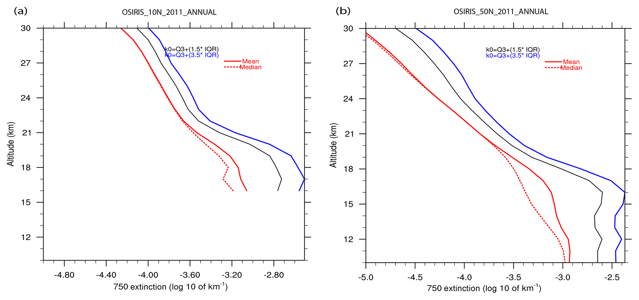
Figure 3Vertical profiles of the OSIRIS version 7.0 level 2 extinction coefficient at 750 nm for the separation of aerosol from enhanced aerosol/cloud values along with the mean and median of extinction before cloud clearing for (a) 10∘ N for 2011; (b) same as in (a) but for 50∘ N.
In our implementation, we use yearly data at each altitude (0.5 km) and latitude (5∘) bin to determine an extinction coefficient probability density function. We used lower quartile (Q1) and upper quartile (Q3) of the underlying distribution to find IQR, which is defined as Q3−Q1, a good measure of the spread in the data relative to median. Here, an extreme outlier is defined as and a more conservative outlier () is used for comparison (Iglewicz and Hoaglin, 1993). A complicating factor is the presence of several small volcanic events during the OSIRIS lifetime and a major pyrocumulus event (August 2017). It is possible that an aggressive outlier process could misidentify measurements of fresh material from either phenomena as cloud events, leading to their erroneous exclusion from the data set. Of course, the very nature of GloSSAC is not conducive to a meaningful depiction of the early evolution of recent volcanic events (Thomason et al., 2018). Figure 2 shows the probability density function of aerosol extinction at 750 nm for two cases in 2011 at 18 km with the threshold used (dashed vertical line) for the outlier detection, whereas Fig. 3 demonstrates vertical profile of threshold values with the mean and median of the distribution. Figure 3 clearly shows the difference between mean and the median profile as the mean profile has higher extinction values in the lower stratosphere due to skewness in the mean statistics. We found that the conservative outlier appeared to remove many enhanced aerosol measurements particularly when stratosphere is perturbed due to volcanic/pyrocumulus events, whereas the extreme outlier was effective at identifying outliers in the density distribution. Therefore we use the extreme outlier to clear cloud-affected observations from the data set.
For SAGE II cloud clearing, we use the ratio of aerosol extinction at two wavelengths (525 and 1020 nm) as a stand-in for aerosol size as well as the magnitude aerosol extinction coefficient. In this space, away from major volcanic events like Pinatubo, clouds manifest a large extinction with a 525-to-1020 nm aerosol extinction ratio near 1. Typical stratospheric aerosol manifests smaller extinction magnitudes and with extinction ratios between 2 and 4. Cloud identification is complicated by mixed fields of view where observations transition between mostly cloudy extinctions and extinction ratios and those more typical of purely aerosol. As a result, the distribution of extinction and extinction ratio shows a continuum between clearly cloud and clearly aerosol observations that makes distinguishing purely aerosol measurements from those affected by cloud ambiguous. Various techniques to parse these mixed measurements have been developed, and GloSSAC makes use of the technique developed by Thomason and Vernier (2013). A similar technique for SAGE III/ISS is in development but not currently available. For this version of GloSSAC, we note that (1) no large volcanic aerosol events have occurred during the SAGE III/ISS mission prior to the end of 2018 and (2) the overall aerosol loading of the stratosphere in this period is low. As a result we can eliminate most observations containing cloud by eliminating all observations where the extinction ratio is less than 2 below 24 km. Given the timing of observations, SAGE III/ISS through 2018 had not observed any polar stratospheric clouds. Not surprisingly, this approach misses some mixed cloud-aerosol observations, but these are effectively identified using the IQR-based cloud detection algorithm used with OSIRIS.
2.3 Comparison of OSIRIS with SAGE II and SAGE III/ISS measurements
Within the GloSSAC paradigm, it is important to not simply observe the agreement between OSIRIS and SAGE II but also mitigate these differences as effectively as possible. We compare SAGE II and OSIRIS once the data have been incorporated into GloSSAC measurement grid: zonally averaged monthly level 3 product at 5∘ latitude and 0.5 km altitude resolution. The OSIRIS version 7.0 standard aerosol product is reported at a wavelength of 750 nm. During the overlap period (2002–2005), we can directly compare these measurements and develop a technique to close observed mutual biases. This technique can then be applied to the entire OSIRIS data record with the assumption that the basic nature of the bias is consistent throughout the period. This is an assumption that may be challenged by a number of small volcanic eruptions occurring during this period which likely change the nature of the aerosol size distribution but for which little means to assess and mitigate are currently available. In addition to 750 nm, OSIRIS extinction can be calculated at 525 nm, a SAGE II measurement wavelength, using a constant Ångström exponent of 2.33 to convert from 750 to 525 nm (Rieger et al., 2015). The one critical exception to this occurs after mid-2017 when the SAGE III/ISS mission begins. SAGE III/ISS makes extinction coefficient measurements at 521 and 756 nm that are near both wavelengths at which OSIRIS reports the extinction coefficient. Since the SAGE III/ISS instruments operate in a manner similar to SAGE II, the expectation is that there would be minimal bias between these instruments at least at the strongest aerosol measurement wavelengths of 525 and 1020 nm.
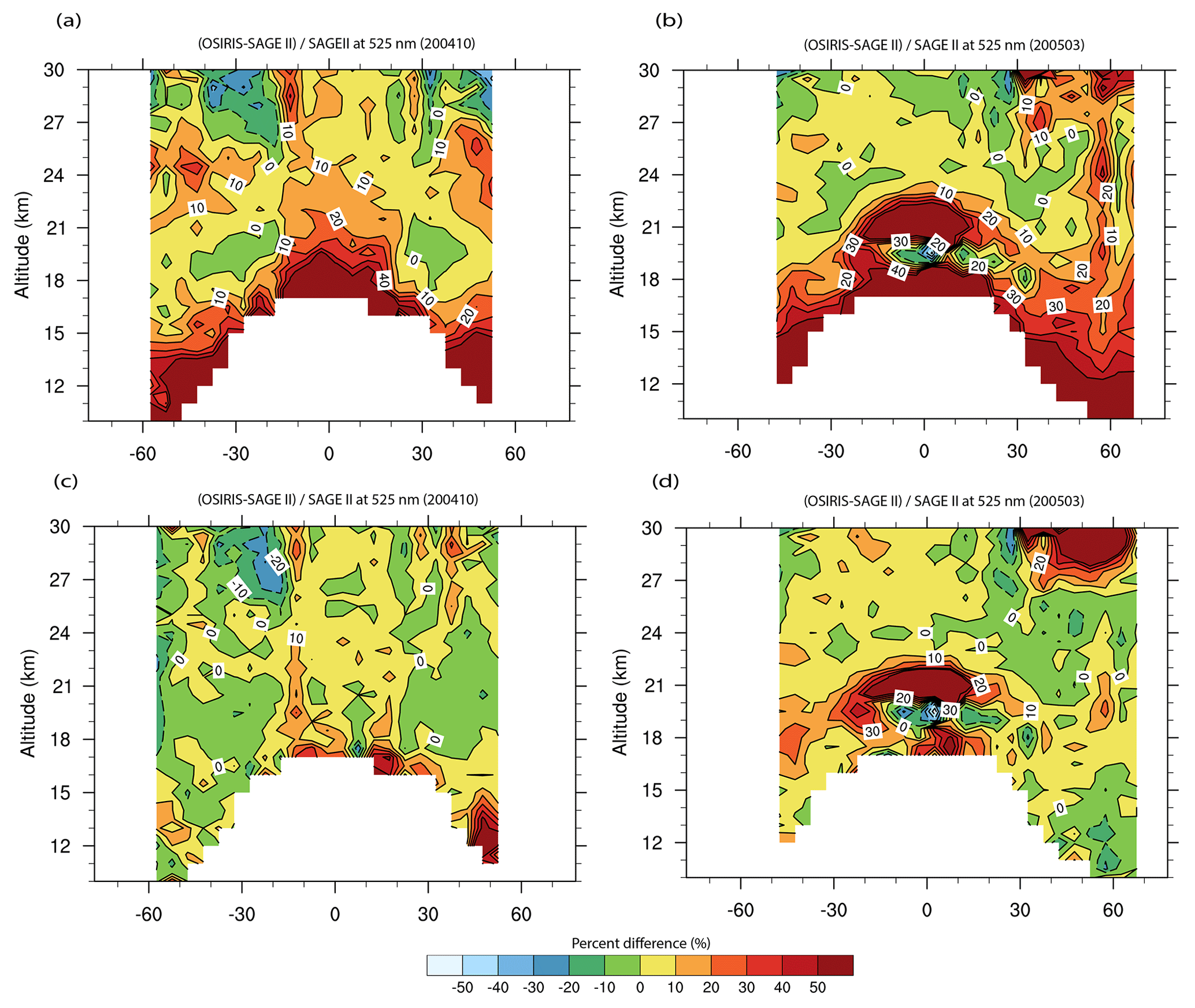
Figure 4Altitude versus latitude of percent difference between the OSIRIS and SAGE II extinction coefficient at 525 nm. Panels (a) and (b) show the percent difference plots for October 2004 and March 2005, for which the OSIRIS extinction coefficient at 525 nm is computed using a constant Ångström exponent of 2.33. Panels (c) and (d) are the same as in (a) and (b) but after implementing a monthly based Ångström exponent to compute OSIRIS extinction at 525 nm.
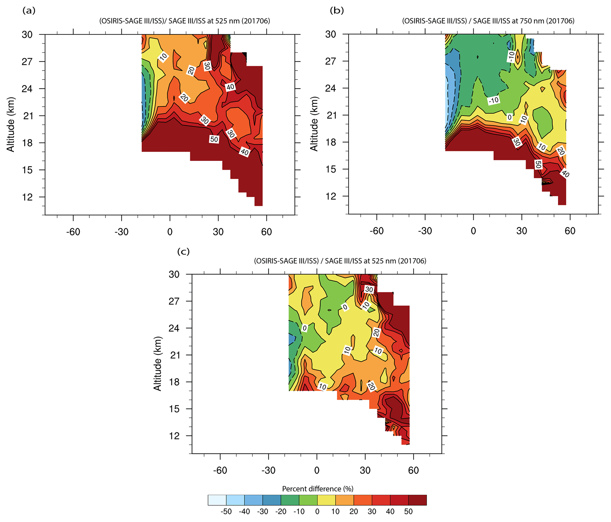
Figure 5Altitude versus latitude of percent difference between the OSIRIS and SAGE III/ISS extinction coefficient (a) at 525 nm for June 2017 and (b) at 750 nm for June 2017. The OSIRIS extinction coefficient used in (a) is computed using a constant Ångström exponent of 2.33, whereas in panel (c) a monthly based pseudo Ångström exponent is used to compute OSIRIS extinction at 525 nm.
A minimal conformance test is that the comparison between SAGE II and OSIRIS in the first overlap period should be very similar to the comparison between SAGE III/ISS during the second overlap period. We expect that the observed correspondence between (i) OSIRIS and (ii) SAGE II and SAGE III/ISS will show this consistency only if (1) the performance of OSIRIS does not change with time1, (2) SAGE II and SAGE III/ISS are relatively unbiased with each other2, and (3) the state of the stratosphere has not changed to the point where it has had a deleterious impact on OSIRIS aerosol retrievals. In Fig. 4a and b, it is apparent that for much of the stratosphere the difference between SAGE II and OSIRIS is less than 10 % particularly in Fig. 4a for a rather benign (less affected by volcanic/fire events) October 2004. However, it is also clear that OSIRIS extinction is consistently higher than SAGE II in the lower stratosphere, with the percentage difference exceeding 50 % near the tropopause. Another departure is shown in Fig. 4b for March 2005 that shows similar features as October 2004. However, in the tropical low and middle stratosphere there is a difference of about 50 % in an enhanced aerosol layer associated with the eruption of Manam in January 2005. Manam is typical of small eruptions observed by SAGE II and later by SAGE III in which a substantial increase in the aerosol extinction coefficient occurs with an increase in the 525-to-1020 nm aerosol extinction ratio. This suggests that extinction is dominated by smaller particles in the volcanic layer than prior to the eruption and is much different than the large extinction/large particle size associated with larger eruptions such as the June 1991 eruption of Pinatubo. Similar small volcano effects are noted in the SAGE II data associated with Ruang in 2002 and by SAGE III/ISS Ambae in July 2018. Figure 5 shows a measurement comparison between June 2017 OSIRIS at 525 nm and SAGE III/ISS at 521 nm (a) and between OSIRIS at 750 nm and SAGE III/ISS at 756 nm (b). Since OSIRIS data are only available through the end of 2017 at this time, relatively few comparative data are currently available. Comparisons between OSIRIS and SAGE III/ISS are complicated in the overlap period by the pyrocumulus fire event in August 2017 which was inhomogeneously distributed in the Northern Hemisphere throughout the second half of 2017. OSIRIS extinction at 750 nm is in reasonable agreement with SAGE III/ISS (b) except in the lower stratosphere and in tropical latitudes where the difference can exceed 20 % in a pattern similar to that seen between SAGE II and OSIRIS (Fig. 5a). However, the differences between OSIRIS at 525 nm and SAGE III/ISS at 521 nm, shown in Fig. 5a, are significantly larger than those seen in Fig. 4a, which suggests either deficiencies in the conversion process of OSIRIS measurements from 750 to 525 nm or that SAGE III/ISS 521 nm data are low biased in the lower and mid-stratosphere at 521 nm though probably not at 756 nm. In general, comparisons of OSIRIS suggest general agreement with both SAGE data sets except in the lower stratosphere where it appears that OSIRIS is biased high relative to the SAGE II and III/ISS measurements. The need for long-term consistency among data sets effectively requires that OSIRIS be brought into conformance (bias reduced as much as possible) with SAGE II measurements.
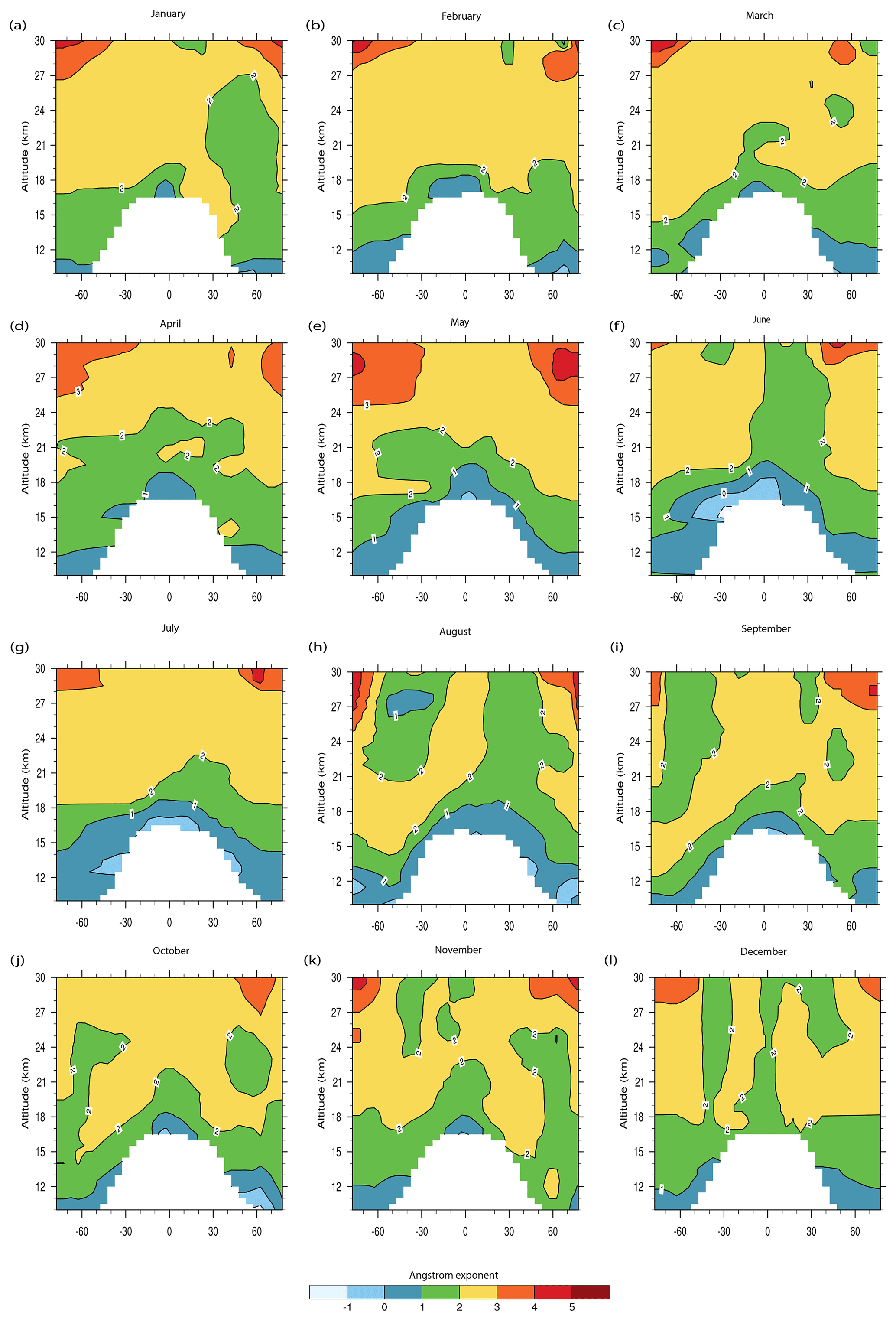
Figure 6Altitude versus latitude of pseudo Ångström exponent monthly climatology derived using OSIRIS 750 nm extinction and SAGE II and SAGE III/ISS 525 nm extinction. A 3×3 median smoothing is used to remove any outliers and then linearly interpolated to fill in any missing data.
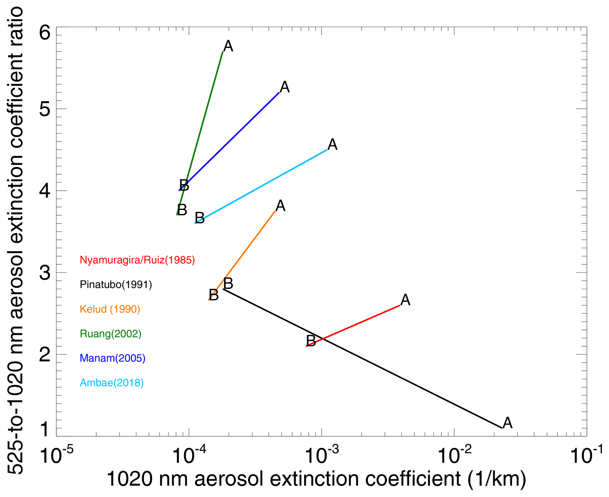
Figure 7The 525-to-1020 nm extinction ratio versus 1020 nm extinction ratio for several volcanic eruptions since 1990. The change in the aerosol extinction coefficient and extinction ratio for each volcanic event is denoted by two points “B” and “A”, which represent the change in the extinction coefficient and extinction ratio before and after eruption.
2.4 OSIRIS extinction coefficient conformance process
Ultimately, the need to reduce the observed differences between SAGE II and OSIRIS is most relevant during the period between the end of the SAGE II mission and the start of the SAGE III/ISS mission. We have developed a mechanism for this in which we have derived a monthly mean Ångström exponent (hereafter “pseudo Ångström exponent”) for the overlap period using SAGE II and SAGE III/ISS 525 nm aerosol extinction with OSIRIS data at 750 nm, effectively creating a 4-year climatology of the pseudo Ångström exponent based on measured values. Within GloSSAC, the Ångström model for aerosol extinction wavelength dependence for 525 and 750 nm is given by
where and are extinctions at 525 and 750 nm respectively; is the pseudo Ångström exponent; and the indices represent year, month, latitude, and altitude respectively. represents ratio of wavelengths at 525 and 750 nm. All data are gridded to 5∘ latitude and 0.5 km altitude resolution. A monthly median climatology of the pseudo Ångström exponent is then computed and smoothed using a 3×3 median boxcar filter in altitude and latitude. Linear interpolation is used to fill in missing values in the monthly grid. Figure 6 shows altitude versus latitude plots of the monthly climatology of the pseudo Ångström exponent and shows a modest annual cycle particularly in the tropical lower stratosphere. While the standard OSIRIS 525 nm aerosol extinction product uses a fixed Ångström exponent of 2.33, we compute values between 1 and 3 for much of the stratosphere and occasionally are less than 0 in the lower tropical stratosphere. We do not assume that the derived value for pseudo Ångström exponent has any physical meaning as it accounts for not just the actual behavior of aerosol but also for potential deficiencies in both data sets, and it is simply a means to push OSIRIS extinction measurements toward those produced by SAGE II. Using this climatology of pseudo Ångström exponent values, we can convert any month of OSIRIS data to 525 nm. For example, using the monthly based pseudo Ångström exponent for October 2004, the agreement between modified OSIRIS and SAGE II is almost entirely below 10 % (Fig. 4c). To some extent this is the expected result though it generally suggests that the pseudo Ångström exponent is reasonably stable throughout the overlap period. However for the March 2005 analysis, OSIRIS predictions for 525 nm remain substantially greater than those measured by SAGE II in the region containing material from the recent Manam eruption (Fig. 4d). This suggests that the changes in the observed Ångström exponent and climatological pseudo Ångström value remain significantly different during this small volcanic event. This is not an issue for GloSSAC for this eruption as SAGE II data are used in this period. However during the period between SAGE II and SAGE III/ISS there are a number of similar small volcanic events that could easily have a similar behavior. Figure 7 demonstrates how a variety of small to very large eruptions manifest themselves in the SAGE II and SAGE III/ISS data record. It shows the 1020 nm extinction coefficient and 525-to-1020 nm aerosol coefficient ratio at the peak extinction following five eruptions (Pinatubo, Nyamuragira/Nevado del Ruiz, Ruang, Manam, Ambae) connected to values that occurred at the same altitude/latitude just prior to the eruption. The Pinatubo eruption, which dominates much of the SAGE II record, is by far the largest event and is the only one where the apparent aerosol size increases with the event (decreased aerosol extinction ratio). Most events in this plot show that aerosol size is apparently smaller after a volcanic event than before the event occurred. Sometimes this is fairly subtle (Nyamuragira/Nevado del Ruiz), but sometimes it can be very pronounced (Ruang). There is a tendency for smaller eruptions to produce a larger extinction ratio, but this is not, for this limited sample, sufficiently well behaved to be considered predictive. The conformance process, as it is currently implemented, would produce horizontal lines in Fig. 7, showing no change in ratio from before an event to afterwards. While this is clearly a shortcoming, we are not able at this time to account for changes in extinction ratio for volcanic events in GloSSAC v2.0, where the data set is based on only one wavelength (either OSIRIS or CALIOP). As a result, it is likely that GloSSAC extinction for small volcanic events during the OSIRIS/CALIOP period will be biased high to an unknown extent. Further study into this period may result in changes in a future version of GloSSAC. The overall conformability of OSIRIS, SAGE II and SAGE III/ISS is ultimately tested by the comparison in Fig. 5c, which shows the comparison of revised OSIRIS 525 nm aerosol extinction coefficient data, as computed using the SAGE II-based pseudo Ångström exponent and the SAGE III/ISS-measured 521 nm aerosol extinction coefficient. In this comparison, we see that differences that were generally larger than 20 % and often in excess of 50 % are now reduced to mostly less than 10 % except at high northern latitudes at higher altitudes. While these differences are larger than those found with SAGE II and OSIRIS, the new conformance process clearly is a better step forward in combining these data sets into a uniform data set.
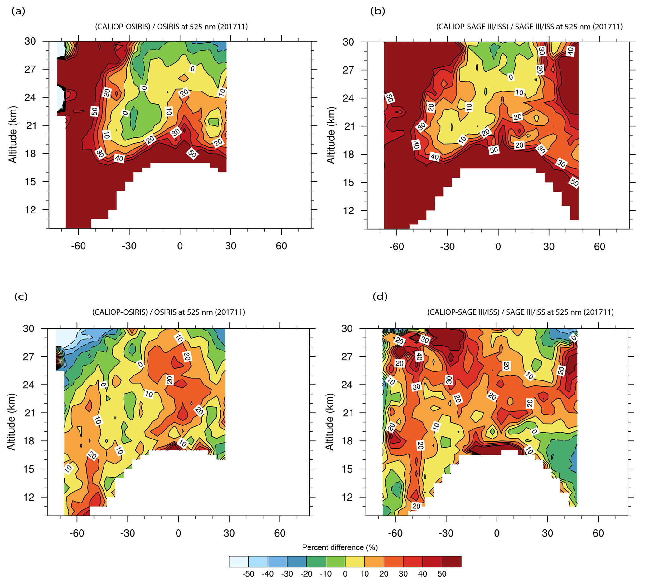
Figure 8Altitude versus latitude of percent difference between CALIOP, OSIRIS and SAGE III/ISS extinction coefficients. Percent difference computed (a) between the CALIOP and bias-corrected OSIRIS extinction coefficient at 525 nm for November 2017 and (b) between the CALIOP and SAGE III/ISS extinction coefficient at 525 nm for November 2017. Panels (c) and (d) are the same as in panels (a) and (b) but CALIOP extinction is bias corrected.
In GloSSAC v1.0, CALIOP and OSIRIS were used as equal partners in which extinction values from each instrument were used where the other was not available and averaged where both existed. Unfortunately, there is no direct overlap between CALIOP and SAGE II mission lifetimes (missing by about 8 months) so that direct comparisons of these data sets is not possible. In v1.0, the CALIOP 532 nm backscatter coefficient was converted to 525 nm extinction using the mean ratio of OSIRIS 525 nm extinction to the CALIOP backscatter coefficient in the GloSSAC data set. This value, 53 sr, is roughly consistent with the extinction-to-backscatter ratio used within CALIOP data processing (50 sr). In v1.0, the CALIOP-converted 525 nm aerosol extinction is roughly consistent with OSIRIS – particularly in producing more aerosol extinction in the lower stratosphere than would be expected based on similar, but in this case not contemporaneous, SAGE II values. As a result, we compare the recently released standard CALIOP extinction coefficient product (Kar et al., 2019) with conformed OSIRIS and SAGE III/ISS data. All three data sets are used at the GloSSAC spatial/temporal resolution. Since CALIOP stratospheric aerosol extinction is reported at 532 nm, a constant Ångström exponent of 2.33 is used here for the conversion of particulate extinction from 532 to 525 nm (an adjustment of 2 %). Figure 8a and b show relative difference plots between (i) OSIRIS and SAGE III/ISS and (ii) CALIOP for November 2017. Equatorward of 30∘ and above roughly 18 km, the differences between the CALIOP extinction product and OSIRIS and SAGE III/ISS are generally between ±20 %. However, the CALIOP standard extinction coefficient product is much larger (>50 %) in the lower stratosphere globally as well as in the entire stratosphere poleward of 40∘ S and 40∘ N. While some of these differences may be attributable to the wildfire-driven pyrocumulonimbus (PyroCb) events (e.g., Peterson et al., 2018), similar discrepancies persist even when the stratosphere is unperturbed by any volcanic/PyroCb events.
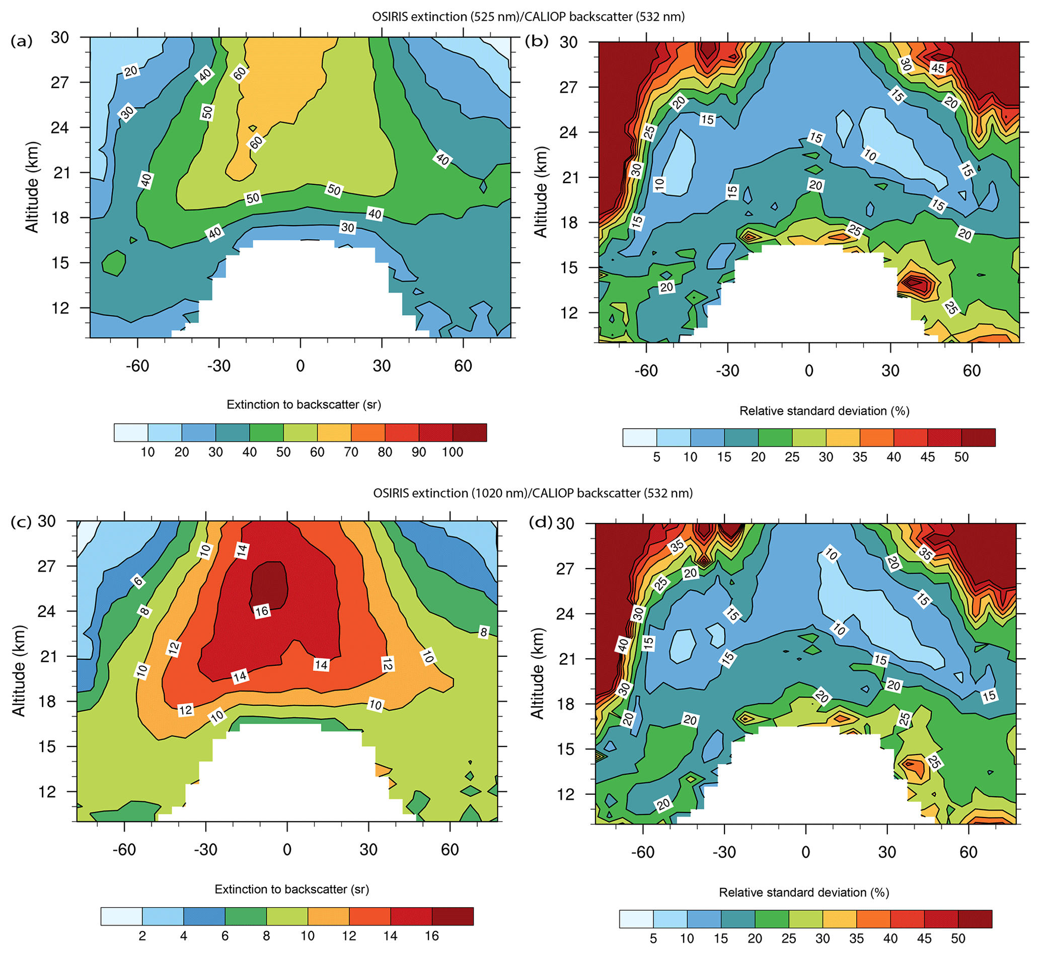
Figure 9Altitude–latitude dependence of median annual OSIRIS extinction to 532 nm backscatter ratio (OSIRIS/CALIOP) for the overlap period (2006–2017). (a) OSIRIS 525 nm extinction to CALIOP 532 backscatter ratio (SF); (b) relative standard deviation of (a) is computed at each grid point with respect to the median value in percent. Panels (c) and (d) are the same as in panels (a) and (b) but using OSIRIS 1020 nm extinction.
Conforming the CALIOP backscatter coefficient to the GloSSAC extinction coefficient
Due to the discrepancy between OSIRIS/SAGE III and CALIOP, we conform CALIOP data using an empirical scaling factor (SF) which is defined as the ratio of bias-corrected OSIRIS extinction at 525 nm and the CALIOP backscatter coefficient at 532 nm. It is analogous to an extinction-to-backscatter coefficient except that it also attempts to account for bias between OSIRIS and CALIOP, and thus the SF should not be viewed as reflecting only underlying aerosol properties. We compute the SF using monthly OSIRIS 525 nm extinction and CALIOP 532 nm particulate backscatter coefficients. The particulate backscatter and extinction products in the standard CALIOP level 3 stratospheric data are retrieved using a lidar ratio of 50 sr (Kar et al., 2019). As we are effectively revising this factor, we do not use products derived using it but rather rederive the backscatter coefficient using the attenuated scattering ratio that is also reported as a part of this product. In this approach, we also assume that the transmission of the atmosphere is close to 1 throughout the stratosphere, which allows us to neglect the attenuation term in the equation of total attenuated backscatter. With this approximation, the particulate backscatter coefficient is computed using the simplified formula , where SR is the scattering ratio and MBKS is the molecular backscatter and is also provided in the CALIOP stratospheric aerosol product. Since the assumption that the transmission of stratosphere is close to 1 is clearly not correct, it is not surprising that the recomputed backscatter coefficient is somewhat less than with the level 3 retrieved particulate backscatter. We find in general that the difference increases with decreasing altitude and is about 10 % at 18 km and close to 30 % at 10 km and that the relative differences exhibit low variance at any given altitude/latitude/time bin. Since, in order to conform the CALIOP data to the conformed OSIRIS data at 525 nm, we are forced to use SFs that are empirical and account for several effects including both aerosol-related effects and bias between the two data sets, it ultimately does not matter a great deal whether we use the standard CALIOP stratospheric backscatter product or the alternative product described above. For GloSSAC v2.0, we choose to use the alternative backscatter product, but users should keep in mind that this choice merely adjusts the size and perhaps the physical meaning of the SF and not the outcome of the 525 nm extinction coefficient estimation. As the CALIOP stratospheric product evolves, we will reconsider the approach in future releases of GloSSAC. Figure 9a shows the annual median of OSIRIS 525 nm extinction to CALIOP 532 nm backscatter ratio as a function of altitude and latitude. Here, the magnitude of the SF varies from between 25 and 65 sr except at higher altitude at polar latitudes where SFs are less than 10 sr. Figure 9b shows the standard deviation for this depiction and we find that the overall behavior of the SF is reasonably consistent throughout the entire period. To implement this conversion process, we use monthly median values of the SF for the entire overlap period for OSIRIS and CALIOP (June 2006 through December 2017) and apply the conversion factors to the entire CALIOP data set at a simple multiplication factor dependent on only latitude and altitude. While it is tempting to infer that CALIOP data processing for this product is using the wrong extinction-to-backscatter ratio, it is important to recall that it seems apparent that CALIOP stratospheric extinction values are biased high compared to OSIRIS conformed data and SAGE III/ISS comparisons by consistent margins in the lower stratosphere and high latitudes where the largest departures of the SF from a value of 50 sr occur. It is worthwhile to note here that Kar et al. (2019) also computed the stratospheric aerosol 532 nm lidar ratio using extinction coefficients from SAGE III/ISS and backscatter measurements from CALIOP for the period June 2017 through August 2018. We note the pattern of their lidar ratio (Fig. 13 of Kar et al., 2019) is more or less consistent with our SF in Fig. 9a.
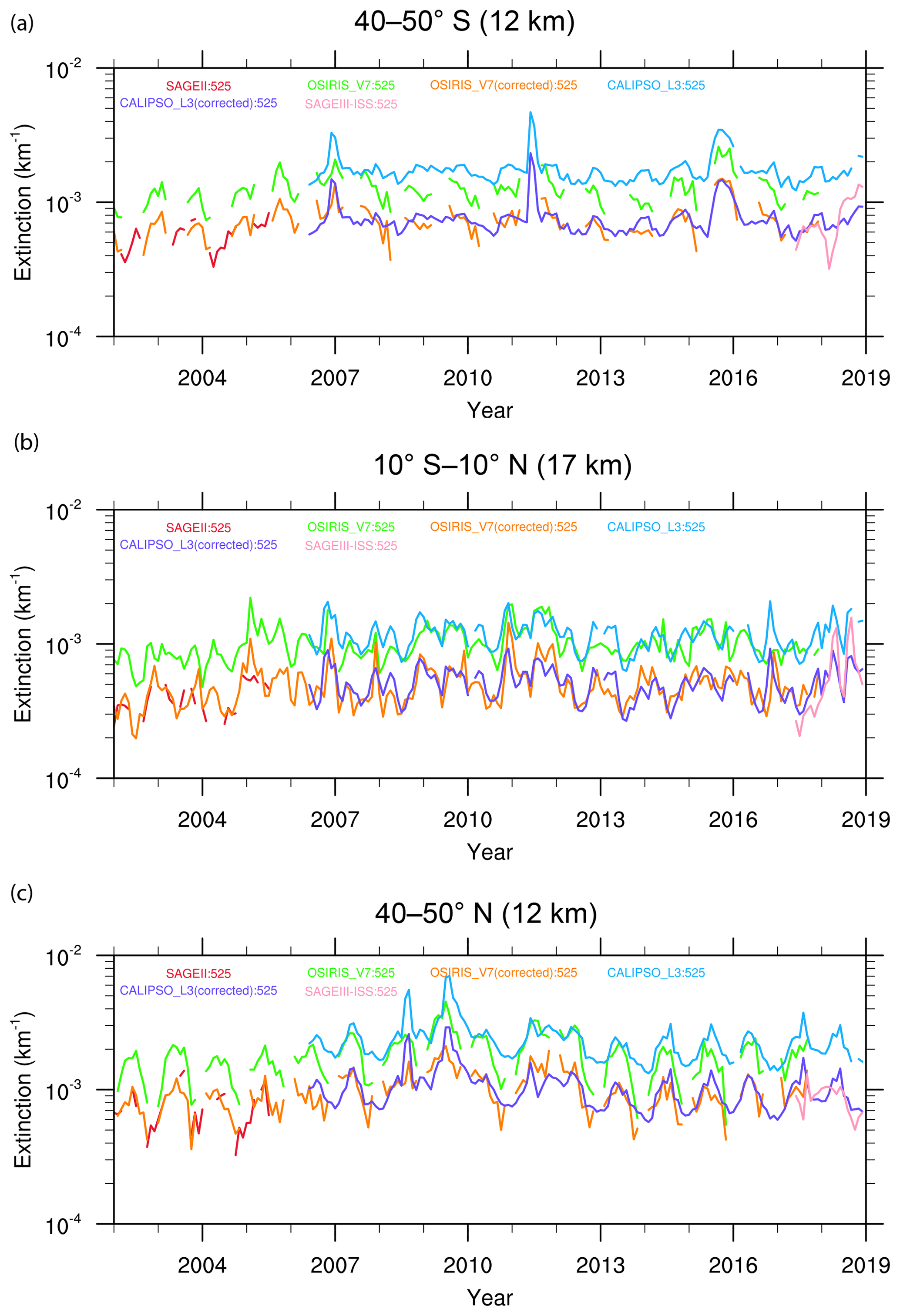
Figure 10Zonally averaged monthly time series plots of the extinction coefficient at 525 nm for different latitude bands and altitudes.
Figure 8 includes the percent difference plots between the empirically scaled CALIOP 525 nm extinction and OSIRIS (c) and SAGE III/ISS (d) for November 2017. It is clear that while the differences are not eliminated, the difference between CALIOP and OSIRIS (Fig. 8c) is now mostly within ±20 %, compared to the standard CALIOP extinction shown in Fig. 8a where the difference between the standard CALIOP stratospheric extinction coefficient and OSIRIS was often more than 50 %. Similarly, the difference between the scaled CALIOP stratospheric extinction and SAGE III/ISS is now mostly below 30 % except near the tropical lower stratosphere and polar high altitudes, whereas the difference between the standard CALIOP stratospheric extinction coefficient and SAGE III/ISS is also often more than 50 %. Figure 10 shows monthly time series of SAGE II, OSIRIS, bias-corrected OSIRIS, CALIOP, bias-corrected CALIOP, and SAGE III/ISS extinction for altitudes and latitudes where conformance has been an issue between the data sets. The time series plots show that (1) the OSIRIS and CALIOP extinction coefficients at 525 nm before conformance are substantially higher than those provided by SAGE II and SAGE III/ISS and (2) these differences are substantially reduced after the conformance process. There are still some clear observations where significant differences among the products exist. Most can be associated with episodic enhancements by a number of small volcanic eruptions (see Table 1) and a major pyrocumulus event in August 2017. Part of these differences may be due to the spatial inhomogeneity of the distribution of aerosol in the first several months following eruptions. However, as previously discussed, the conformance processes applied to OSIRIS and CALIOP cannot adequately account for fresh aerosol from these events. Nonetheless, given the status of OSIRIS/CALIOP/SAGE conformance in GloSSAC v1.0, the process used in the new version represents an imperfect step forward.
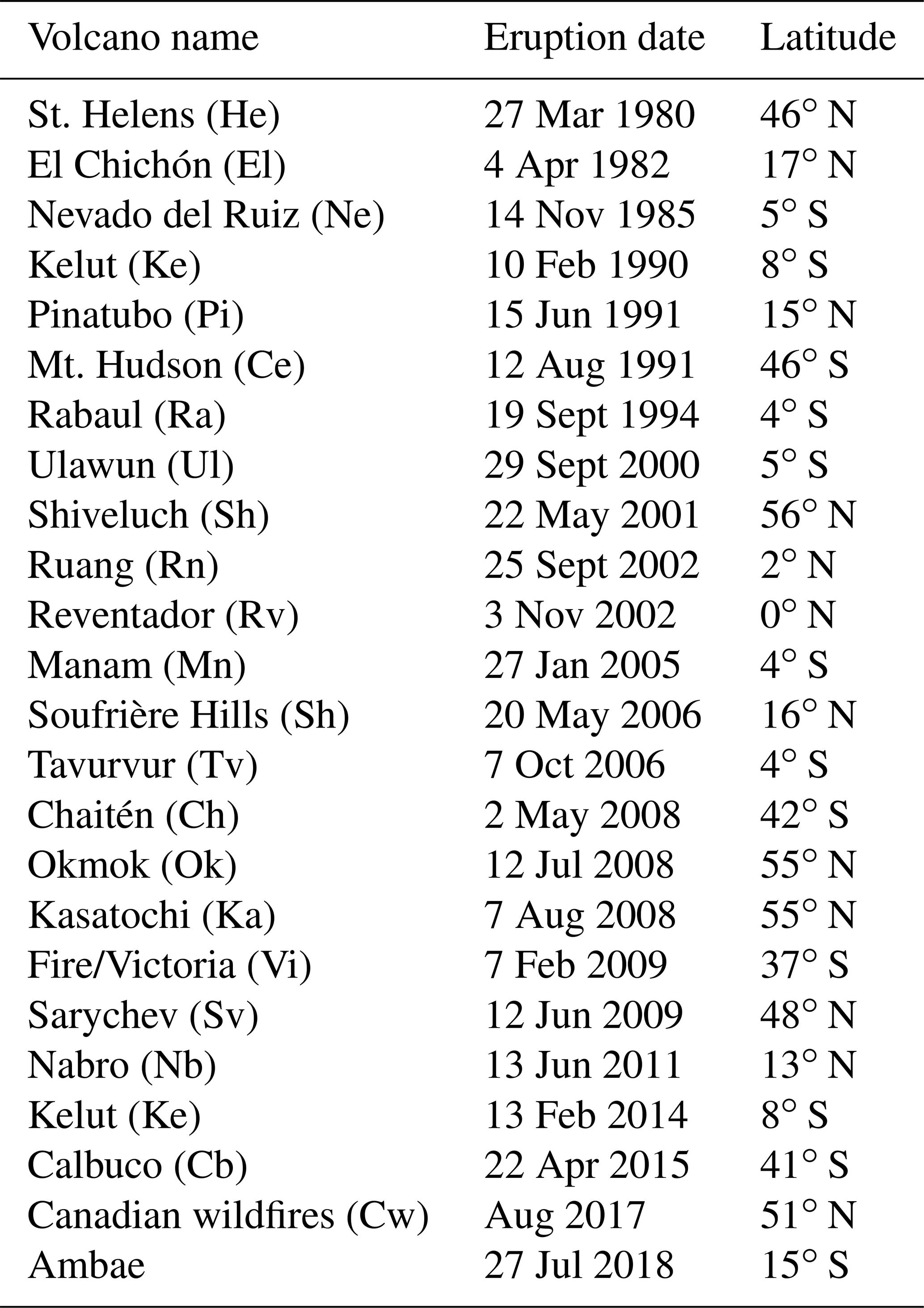
Table 1List of significant volcanic eruptions/wild fire events that occurred during the entire record of GloSSAC.
For GloSSAC v1.0 (Thomason et al., 2018), extinction measurements at 525 and 1020 nm were included in the stratospheric aerosol record. The post-SAGE II record was focused on producing a uniform extinction coefficient record at 525 nm, and the aerosol extinction coefficient at 1020 nm was inferred using an empirical relationship between the 525-to-1020 nm extinction ratio and the 525 nm extinction derived from SAGE II data. However, this process was not fully successful, and a noteworthy bias between the SAGE II and post-SAGE II period at 1020 nm was observed in v1.0 (Thomason et al., 2018), leading to recommendations to avoid using 1020 data in the v1.0 data set in the post-SAGE II part of the record. For GloSSAC v2.0, we use a different strategy focused on using monthly pseudo Ångström exponents computed using measurements between (i) OSIRIS and (ii) SAGE II and SAGE III/ISS that is functionally identical to the method used in Sect. 4.2 to infer extinction at 525 nm from OSIRIS. We produce a monthly average of the pseudo Ångström exponent using the SAGE II and SAGE III/ISS 1020 nm and OSIRIS 750 nm extinction coefficient (Fig. 11). Generally, we would expect to derive a similar pseudo Ångström exponent for the 750 to 1020 nm conversion as used in the case of inferring OSIRIS 525 nm extinction from the SAGE II 525 nm extinction coefficient. However we find, particularly in the lower stratosphere, significantly larger exponents for the 750-to-525 nm extinction conversion than for the 750-to-1020 nm conversion. For instance, in the lower tropical stratosphere, we find values for the former as large as 0, whereas as comparable values for the latter are less than −3.

Figure 11Altitude versus latitude of the pseudo Ångström exponent monthly climatology derived using OSIRIS 750 nm extinction and SAGE II and SAGE III/ISS 1020 nm extinction. A 3×3 median smoothing is used to remove any outliers and is then linearly interpolated to fill in any missing data.
We use these monthly pseudo Ångström exponents to infer an OSIRIS extinction coefficient product at 1020 nm for the post-SAGE II period. Again, we do not propose these exponents as having only information regarding aerosol optical properties as they also account for systematic differences between aerosol data products. These empirical parameters are simply what are required to bring OSIRIS aerosol extinction data into conformance with SAGE II/III data and fulfill the goals of GloSSAC v2.0. In order to infer the 1020 nm extinction coefficient from CALIOP 532 nm backscatter data, we follow the same procedure as we employed to infer CALIOP 525 nm extinction in Sect. 5.1. Figure 9c shows the annual median of OSIRIS extinction at 1020 nm to CALIOP 532 nm backscatter ratio. Despite whatever shortcomings these values may have relative to reflecting aerosol properties, we use these ratios to compute CALIOP extinction at 1020 nm.
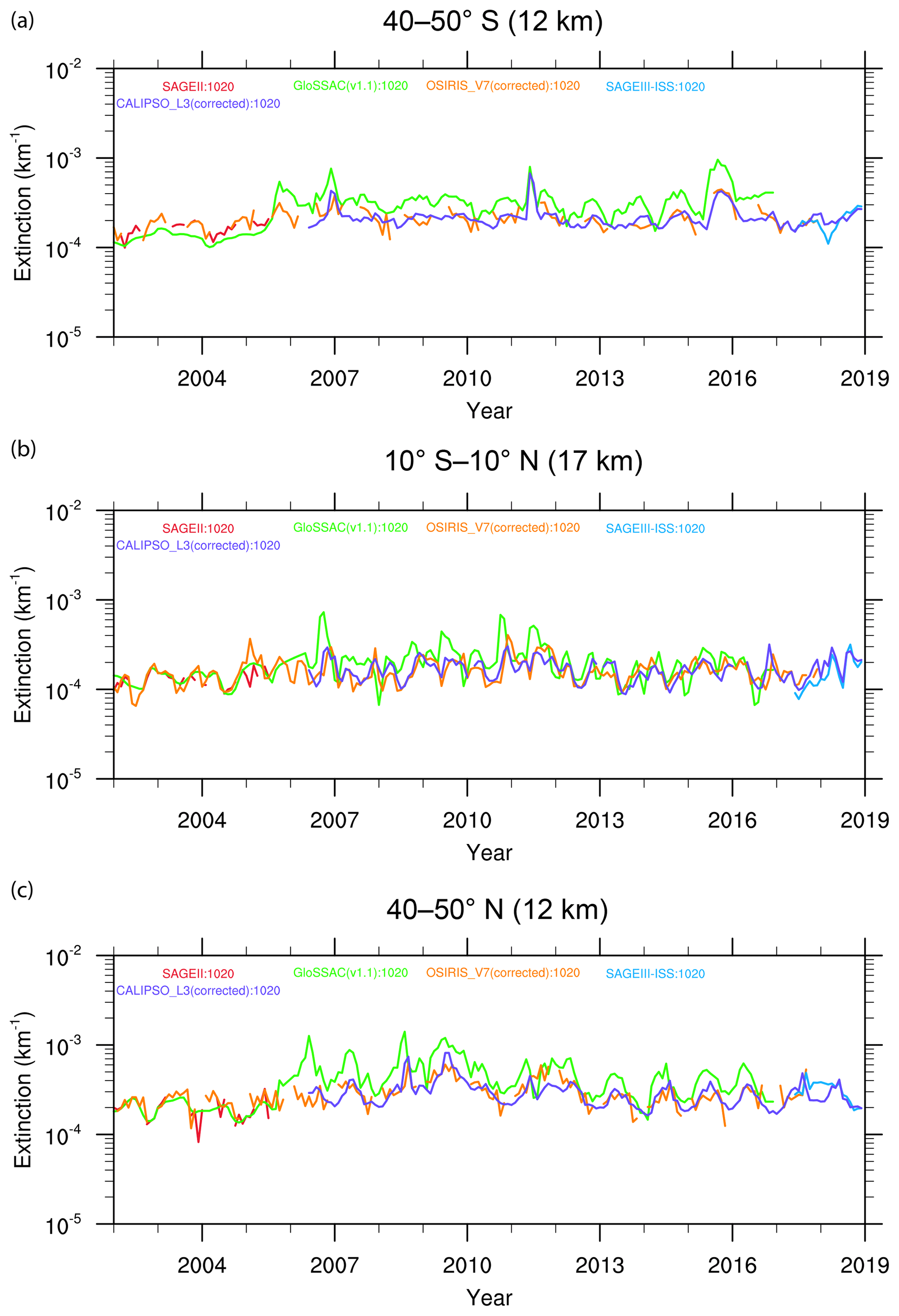
Figure 12Zonally averaged monthly time series plots of the extinction coefficient at 1020 nm for different latitude bands and altitudes.
Figure 12 shows the monthly time series for SAGE II and SAGE III/ISS as well as conformed OSIRIS and CALIOP data at some lower stratospheric levels. We find that OSIRIS 1020 nm extinction is in reasonable agreement with the SAGE II and SAGE III/ISS 1020 nm extinction coefficient, with an overall agreement between (i) OSIRIS and (ii) SAGE II and SAGE III/ISS of ±20 %. It should be noted that there are still some significant outliers between SAGE products and the converted OSIRIS values almost always associated with significant increases in the stratospheric aerosol burden such as those following the Manam volcanic eruption in January 2005, where apparent changes in aerosol size may be playing an outsized role. Figure 12 further shows that CALIOP 1020 nm extinction fits in reasonably well with OSIRIS and SAGE III/ISS, suggesting that the inferred 1020 nm extinction is fairly robust. It should also be noted that, in some cases (particularly for February 2016 and October 2018) when no CALIOP data are available, we linearly interpolate CALIOP data in time between January (September) and March (November) of 2016 (2018) to fill in the missing monthly data following methods used in interpolating SAGE II data. In GloSSAC version 2.0, the data between August 2005 (after the SAGE II mission ends) and June 2006 (CALIOP mission starts), the only data set available is OSIRIS, and there are cases when missing data in OSIRIS need to be filled. In such cases, we either use the closest month data or a linear interpolation when there are more than two consecutive months of data available at each grid point, while assuring the consistency and continuity in the merged data. SAGE III/ISS data are incorporated into the extinction record from June 2017, and we prioritize SAGE III/ISS data over OSIRIS and CALIOP whenever SAGE III/ISS data are available. Figures 13 and 14 show extinction from bias-corrected 525 and 1020 nm respectively for OSIRIS, CALIOP, SAGE III/ISS and merged extinction at 47.5∘ N latitude. Overall, the continuity in the data is maintained after merging different data sets. Uncertainties related to each variable are also included in the final data product (see Supplement on how uncertainties are estimated).
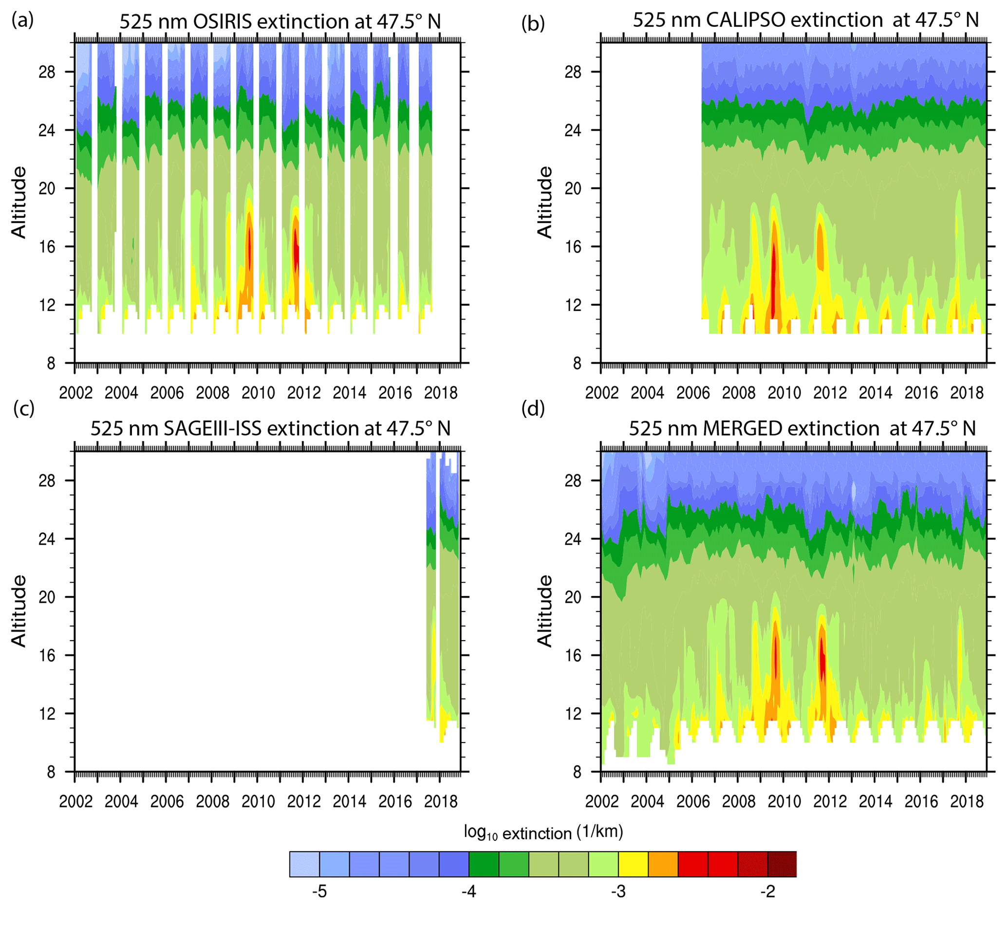
Figure 13Altitude versus monthly time series of the 525 nm extinction coefficient at 47.5∘N latitude. (a) Bias-corrected OSIRIS extinction coefficient, (b) bias-corrected CALIOP extinction coefficient, (c) cloud-cleared SAGE III/ISS extinction coefficient and (d) final merged 525 nm GloSSAC v2.0 extinction coefficient.

Figure 14Altitude versus monthly time series of the 1020 nm extinction coefficient at 47.5∘ N latitude. (a) Bias-corrected OSIRIS extinction coefficient, (b) bias-corrected CALIOP extinction coefficient, (c) cloud-cleared SAGE III/ISS extinction coefficient and (d) final merged 1020 nm GloSSAC v2.0 extinction coefficient.
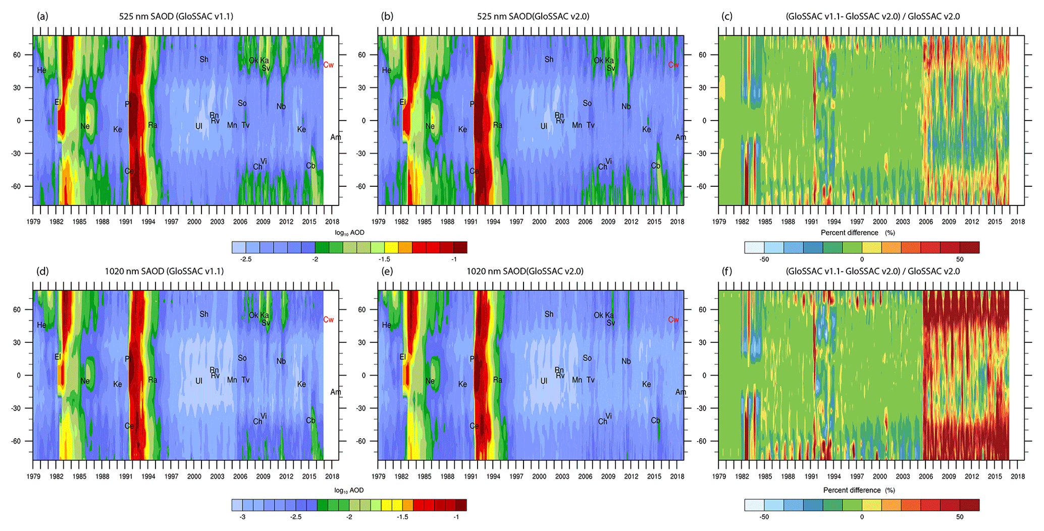
Figure 15Latitude versus monthly time series of SAOD at 525 and 1020 nm: (a) using GloSSAC v1.0; (b) using merged OSIRIS bias-corrected version 7.0, bias-corrected CALIOP, and SAGE III/ISS data (GloSSAC 2.0); and (c) percent difference between (a) and (b). Panels (d), (e), and (f) are same as (a), (b), and (c) but for 1020 nm extinction. For 525 nm extinction, OSIRIS data are bias corrected using monthly pseudo Ångström exponents shown in Fig. 5, while CALIOP 525 nm extinction is inferred using the OSIRIS 525 nm extinction to CALIOP 532 nm backscatter ratio. For 1020 nm, OSIRIS data are bias corrected using monthly pseudo Ångström exponents shown in Fig. 11, while CALIOP 1020 nm extinction is inferred using the OSIRIS 1020 nm extinction to CALIOP 532 nm backscatter ratio.
A formal stratospheric aerosol optical depth (SAOD) at 525 and 1020 nm is included in GloSSAC v2.0. We compute SAOD by integrating aerosol extinction at respective wavelengths from the monthly average tropopause in the data set to 40 km following the method described in Thomason et al. (2018). Figure 15 shows latitude versus monthly time series of SAOD from GloSSAC v1.1, this version (v2.0), and the difference between v2.0 and v1.1 for the entire 40-year record that depicts major and minor volcanic eruptions. Figure 15a shows a consistent 525 nm optical depth enhancement at mid- and high latitudes across the transition between SAGE II and OSIRIS in August 2005, which is a reflection of the lower stratospheric discrepancy observed in previous versions. Thomason et al. (2018) suggested that this could be related to the January 2005 eruption of Manam but also recognized that it may be an instrumental artifact. We show SAOD from the merged GloSSAC v2.0 data in Fig. 15b, where updated versions of OSIRIS and CALIOP data have been conformed to SAGE II (CALIOP indirectly so), and we now include data from SAGE III/ISS. The relative difference between GloSSAC 2.0 and GloSSAC 1.1 is shown in Fig. 15c. It is evident from Fig. 15c that the smallest difference between version 2.0 and v1.1 occurs in the Southern Hemisphere, while in Northern Hemispheric higher latitudes the difference is between 10 % and 40 %. Compared to the optical depths shown in Fig. 15a and b, it is clear that while some enhancement after 2005 remains it is substantially smaller than in v1.1. For the period between 1979 and 2005, the differences between version 1.1 and 2.0 are seen during and following the El Chichón (1982) and Pinatubo (1991) eruptions. The increase in percent difference in 1991 is mostly driven by a change in version 2.0 to not interpolate from May to July in SAGE II data.
At 1020 nm, the SAOD was noted as a deficiency in v1.0 as the conformance process did not produce satisfactory results for this period. In Fig. 15d, it is clear that there is a much larger discontinuity across the instrument transition in 2005 at 1020 nm than at 525 nm. In Fig. 15e, we observe that evidence for a discontinuity across the instrument change in 2005 is significantly reduced, and, in fact, it is not clear that one exists at all. The differences in the two versions is shown in Fig. 15f, where we find that the optical depth for this period is reduced by as much as 50 % at high latitudes.

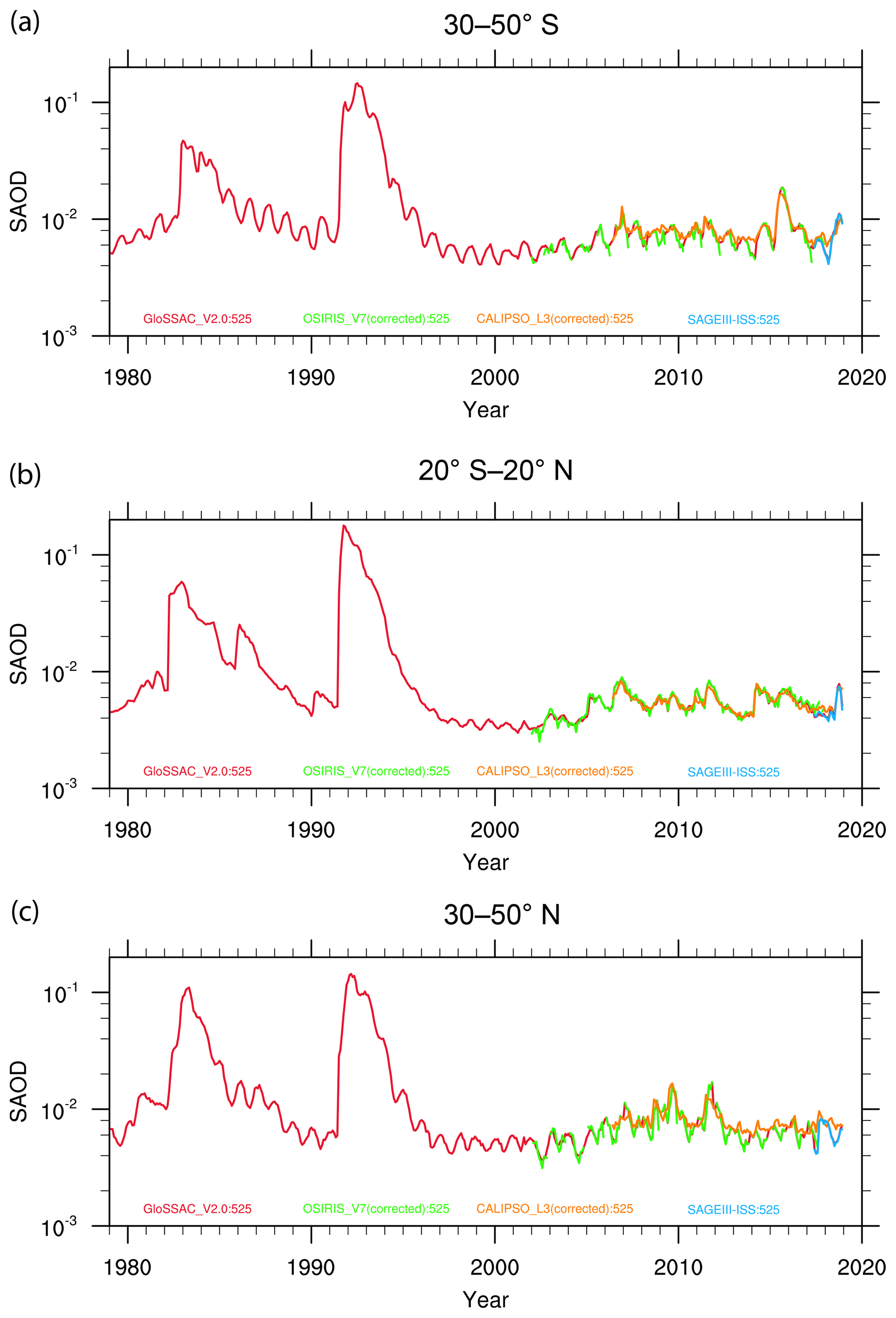
Figure 17Zonally averaged monthly stratospheric aerosol optical depth at 525 nm for (a) 30–50∘ S, (b) 20∘ S–20∘ N, and (c) 30–50∘ N.
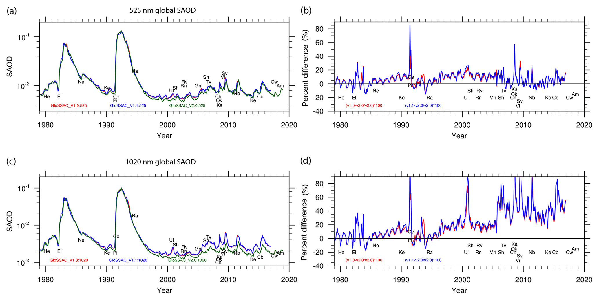
Figure 18Global stratospheric aerosol optical depth at 525 (a) and 1020 nm (c). Percent difference between versions for 525 and 1020 nm extinction are shown in (b) and (c) respectively. Percent difference are computed with respect to v2.0 as (v1.0 .
Figure 16 shows a similar plot but for version 1.0 and 2.0. The significant differences between version 1.0 and 2.0 remain somewhat similar to differences between v1.1 and 2.0 shown in Fig. 15. Figure 17 shows monthly time series of GloSSAC v2.0 SAOD at 525 nm for three different latitude bands for the entire 40-year record. Signatures of major volcanic eruptions (e.g., El Chichón in 1982 and Mount Pinatubo in 1991) and several other minor volcanic eruptions as listed in Table 1 in the post-SAGE II era are clearly evident in Fig. 17. Figure 17 also shows how individual measurements of OSIRIS, CALIOP and SAGE III/ISS contribute toward the post-SAGE II aerosol record of GloSSAC v2.0. Additionally, a global SAOD time series for the entire record is shown in Fig. 18. The percent difference of global SAOD of earlier versions with respect to v2.0 is shown in Fig. 18b and d. The largest percent difference in SAOD occurs in June 1991 in both 525 and 1020 nm percent difference plots (b, d), which is due to a change in version 2.0 of GloSSAC to not to interpolate from May to July in SAGE II extinction coefficient data that are related to the usage of CLAES data. The difference in SAOD in the post-SAGE II period (after 2005) is due to the changes in version 2.0, which has improved over the older versions. This difference is mostly due to a reduction of SAOD at higher latitudes as is evident from Fig. 15c and f. For 1020, the difference between older versions and version 2.0 is much larger because of the reduction in discontinuity across instruments due to the conformance process used in version 2.0. We also note that in Fig. 18d the SAOD has significantly reduced (as much as 50 % or more) for 1020 nm as is evident in Fig. 15f as well. These differences may have implications on climate modeling as one of the recent modeling studies (Rieger et al., 2020) shows that the difference between v3.0 and v4.0 of CMIP6 stratospheric aerosol data that are derived from v1.0 and v1.1 of GloSSAC causes a reduction in instantaneous top-of-the-atmosphere radiative forcing following the Pinatubo eruption.
As with v1.0, we cannot exclude the possibility that ongoing volcanic activity plays a dominant role in the apparent enhancement after 2005. This possibility is bolstered by noting that optical depths shown in Fig. 15b and e approach those observed in 2004, 2013 and early 2014 during a lull in a decade of repeated minor volcanic stratospheric enhancements. We also note that several recent modeling studies (e.g., Schmidt et al., 2018; Aubry et al., 2020) using sulfur dioxide emissions in aerosol-climate models have reported an enhancement in SAOD for the post-2005 time period. Nevertheless, we cannot exclude the possibility that some bias across the transition between SAGE II and the OSIRIS/CALIOP period continues to exist. It is possible that, with further overlap between SAGE III/ISS and OSIRIS and CALIOP, a better understanding of instrumental differences will permit a more robust conformance process for future versions of GloSSAC.
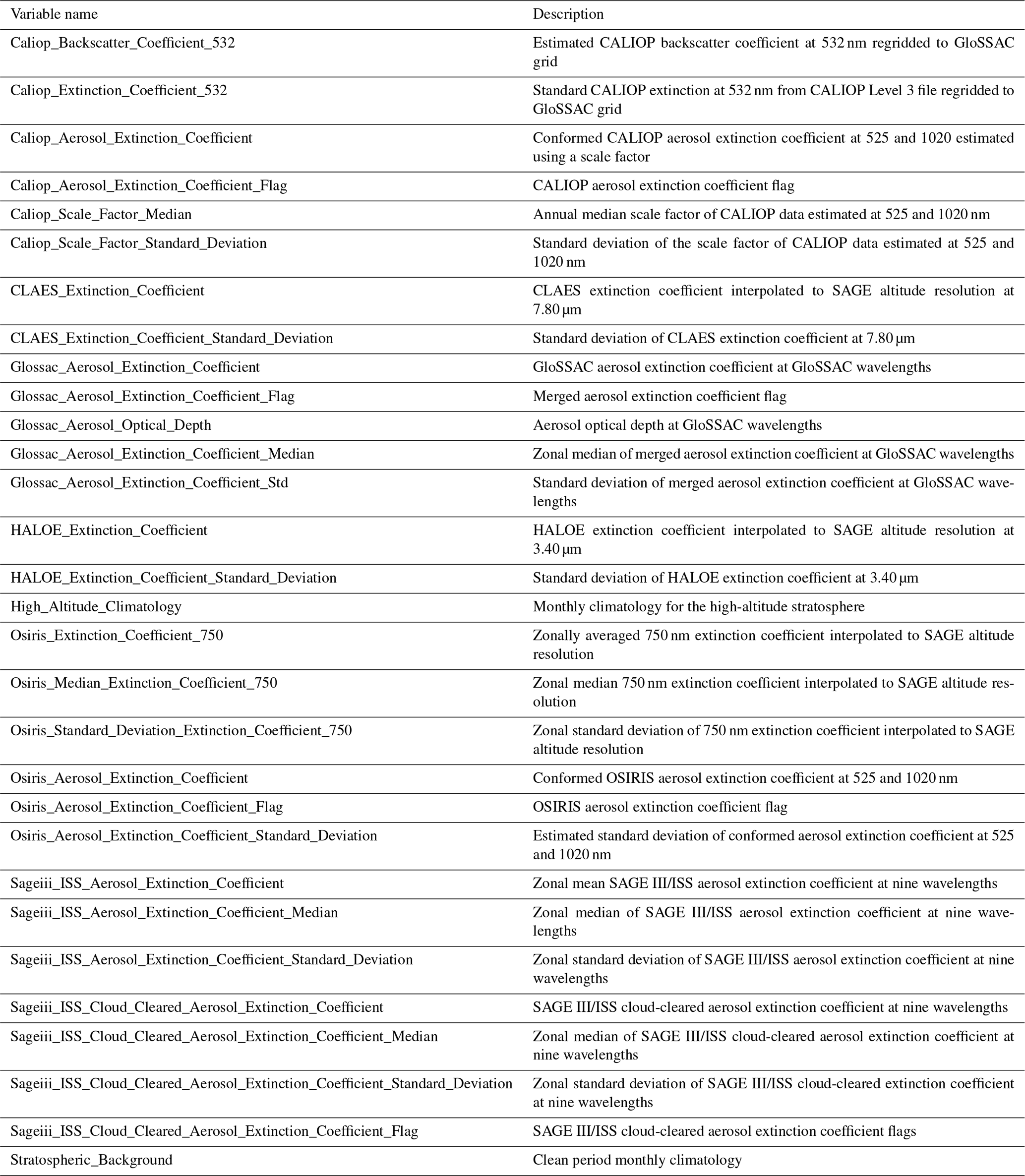
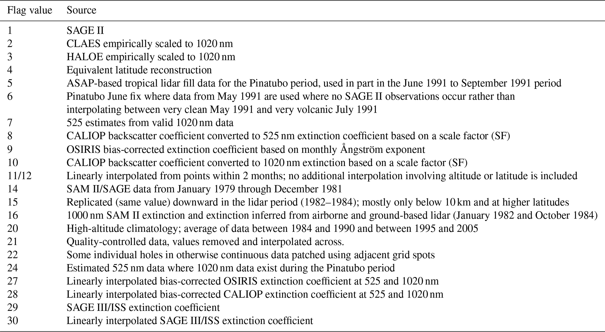
The contents of the GloSSAC v2.0 netCDF file are similar to those for v1.0. Some additional data records include gridded SAGE III/ISS data at nine wavelengths and the original unconformed data for CLAES, HALOE, OSIRIS and CALIOP. All space-based data sets include the median reported uncertainty and the zonal standard deviation for each instrument product and for its conformed version in each altitude/latitude/time bin in which data are available. Version 2.0 also includes SAOD at 525 and 1020 nm. The contents of the GloSSAC v2.0 netCDF file are listed in Table B1 with variable name and description. Table B2 lists the data flag values associated with the data set.
The GloSSAC v2.0 netCDF file is available from the NASA Atmospheric Data Center (https://asdc.larc.nasa.gov/data/GloSSAC/GloSSAC_V2.0.nc) and referenced using its DOI: https://doi.org/10.5067/glossac-l3-v2.0 (Thomason, 2020).
Here we present v2.0 of GloSSAC that extends from 1979 through 2018 with the addition of new SAGE III/ISS data toward the end of the record and with some changes to the data used in the post-SAGE II era. We now use OSIRIS version 7.0 data (Rieger et al., 2019) instead of version 5.07, which was used in GloSSAC v1.0. The OSIRIS version 7.0 data are improved in terms of data quality in the lower stratosphere. However, the bias in the lower stratosphere is not entirely resolved as higher percent differences still exist between (i) OSIRIS and (ii) SAGE II and SAGE III/ISS. Here, we use a conformance process to reduce the observed differences between (i) OSIRIS and (ii) SAGE II and SAGE III/ISS, which is based on the monthly pseudo Ångström exponent computed using 750 nm OSIRIS extinction and 525 nm SAGE II and SAGE III/ISS extinction coefficients. A similar approach is implemented for inferring the 1020 nm extinction coefficient. We continue to make use of CALIOP data in this version as well with some changes. At the time of development of GloSSAC v1.0, there was no standard stratospheric aerosol product available from CALIOP, and we therefore used its version 4.0 level 1 aerosol backscatter coefficient product at 532 nm and identified and removed observations that suggested the presence of cloud using the depolarization measurement (Vernier et al., 2009; Thomason et al., 2018). The cloud-cleared backscatter coefficients were then compiled into the spatial temporal resolution used in GloSSAC (monthly, 5∘ latitude bins and 0.5 km altitude bins). Now that the CALIPSO standard stratospheric aerosol product (Kar et al., 2019) is available, we use the standard stratospheric aerosol product. However, we note that standard CALIOP aerosol extinction coefficients computed at 525 nm tend to overestimate aerosol extinction in the lower stratosphere globally as well as in the entire stratosphere poleward of 40∘ S and 40∘ N. We therefore use a SF based on the conformed OSIRIS extinction coefficient and CALIOP-estimated backscatter to conform the CALIOP data. The conformed CALIOP extinction coefficient is in reasonable agreement with OSIRIS and SAGE III/ISS with some exceptions. These changes resulted in an improved version 2.0 data. Some important changes in version 2.0 include the change in the usage of CLAES data during the Pinatubo time period that resulted in a reduction of the extinction coefficient following the Pinatubo eruption and improved extinction coefficients in the post-SAGE II era data. These changes in version 2.0 reflect in 525 nm SAOD data as about an 80 % reduction of SAOD occurs in June 1991 when compared against previous versions due to changes in the usage of CLAES data, whereas in the post-SAGE II period we note no significant change in SAOD at 525 nm. However, for 1020 nm extinction we note a significant improvement in the post-SAGE II era that results in significant reduction (as much as 50 % or more) of SAOD in version 2.0 due to the new conformance process based on monthly Ångström exponent, where we observe that evidence for a discontinuity across the instrument change in 2005 is significantly reduced. Overall, the quality and robustness of the stratospheric aerosol product have improved for GloSSAC v2.0 with some issues that still persist in the data set which we mention below.
-
Despite using a monthly based measured pseudo Ångström exponent in converting OSIRIS extinction from its native wavelength of 750 to 525 nm, we note that this method has its own limitations during periods when the stratosphere is perturbed due to volcanoes/PyroCb events. The OSIRIS 525 nm extinction coefficient is somewhat biased high in such events where we have SAGE II and SAGE III/ISS data to compare. Although the monthly based pseudo Ångström exponent correction significantly improves the comparison between OSIRIS and SAGE II extinction at 525 nm, we note somewhat large percent differences (>20 %) between OSIRIS and SAGE II following the Manam eruption (Fig. 4d). Similar instances are also noted when both data are available and more so in the tropical latitudes between 20∘ S and 20∘ N. We unfortunately do not have SAGE II measurements after August 2005 to validate OSIRIS data. However, toward the end of the record we use SAGE III/ISS to validate OSIRIS and CALIOP. For this time period, the agreement between the SAGE III/ISS and OSIRIS/CALIOP extinction coefficient is mostly within ±20 % but degrades somewhat during and following Canadian PyroCb events in 2017. Coincident OSIRIS and SAGE III/ISS measurements during this time period are studied in Bourassa et al. (2019).
-
Since we use CALIOP stratospheric aerosol data to fill in missing OSIRIS data for the time period from June 2006 onward, issues pertaining to CALIOP data should also be mentioned. The standard CALIOP stratospheric aerosol product provides the backscatter coefficient as it needs to be converted to the extinction coefficient at the wavelength of interest for the GloSSAC usage. The standard CALIOP product also provides extinction at 532 nm. However, we note that the CALIOP standard extinction product is biased high when compared against SAGE III/ISS and OSIRIS (Fig. 8a, b). We therefore compute particulate backscatter from the scattering ratio and molecular backscatter coefficient and further infer the extinction coefficient using an altitude–latitude-based scale factor (SF) which is derived from the conformed OSIRIS extinction coefficient and estimated CALIOP backscatter coefficient. With this bias correction, bias between OSIRIS and corrected CALIOP extinction has now been reduced. However, it should also be noted that any bias in OSIRIS data will be reflected in CALIOP-inferred extinction as we use OSIRIS extinction in the conversion process. While it gives us confidence in both bias-corrected OSIRIS and CALIOP extinction in comparison with SAGE III/ISS that the differences between these data sets are mostly within ±20 %, the representation of the aerosol extinction coefficient particularly during small volcanic eruptions that occurred during the OSIRIS/CALIOP period (2006–2017) is still a challenge with single-wavelength measurements (either OSIRIS or CALIOP). We also note that the bias in the lower stratosphere is not entirely resolved as differences still exist between OSIRIS/CALIOP and SAGE measurements.
-
While the inferred 1020 nm extinction in GloSSAC v2.0 for the post-SAGE II era (2005–2018) is improved compared to v1.0, there are limitations with the 1020 nm extinction. We note that deducing size information using the 525 and 1020 nm extinction ratio for the period between August 2005 and June 2017 may still be an issue with single-wavelength measurement from either OSIRIS or CALIOP, particularly during and following a volcanic event, despite some improvement in the inferred 1020 nm extinction. While this is clearly a limitation, we are not able to address changes in extinction ratio for volcanic events in v2.0, where the data set is based on only one wavelength. As a result, it is likely that GloSSAC extinction for small volcanic events during the OSIRIS/CALIOP period will be biased high to an unknown extent. Further study into this period may result in changes in a future version of GloSSAC. Since June 2017, multiwavelength extinction coefficient data became available from SAGE III/ISS, giving us an opportunity to compare/validate OSIRIS/CALIOP data particularly during and following such events.
There are additional data sets that are available for stratospheric aerosol extinction coefficients. We plan to evaluate and use these data sets, including the SCanning Imaging Absorption spectroMeter for Atmospheric CHartographY (SCIAMACHY) and Ozone Mapping Profiler Suite (OMPS).
| ASAP | Assessment of Stratospheric Aerosol Properties |
| CALIOP | Cloud-Aerosol Lidar with Orthogonal Polarization |
| CALIPSO | Cloud-Aerosol Lidar and Infrared Pathfinder Satellite Observation |
| CCM | chemistry-climate model |
| CCMI | Chemistry-Climate Model Initiative |
| CLAES | Cryogenic Limb Array Etalon Spectrometer |
| CMIP | Coupled Model Intercomparison Project |
| CMIP6 | Coupled Model Intercomparison Project version 6 |
| GCM | global climate model |
| GloSSAC | Global Space-based Stratospheric Aerosol Climatology |
| HALOE | Halogen Occultation Experiment |
| ISS | International Space Station |
| NASA | National Aeronautics and Space Administration |
| NAT | nitric acid trihydrate |
| OSIRIS | Optical Spectrograph and InfraRed Imager System |
| PSC | polar stratospheric cloud |
| SAGE | Stratospheric Aerosol and Gas Experiment |
| SF | scale factor |
| SPARC | Stratospheric-tropospheric Processes and their Role in Climate |
| STS | saturated ternary solution |
| SSiRC | Stratospheric Sulfur and its Role in Climate |
| VEI | Volcanic Eruption Index |
| WCRP | World Climate Research Programme |
The supplement related to this article is available online at: https://doi.org/10.5194/essd-12-2607-2020-supplement.
MK and LWT conceived the idea and methodology used in this paper. MK carried out the analysis, while NE helped with version 1.1 of the data (data prior to 2001). LR and AB provided us with version 7.0 of OSIRIS data and participated in the scientific discussion in regard to OSIRIS data in particular. LM provided help with the equivalent latitude that was used in filling data for the SAGE II era. MK wrote the manuscript, while all authors reviewed the manuscript and provided advice on the manuscript and figures.
The authors declare that they have no conflict of interest.
We acknowledge the support of NASA Science Mission Directorate and the SAGE II and III/ISS mission teams. The SAGE mission is supported by the NASA Science Mission Directorate. SSAI personnel are supported through the STARSS III contract. Contributions by Adam Bourassa and Landon Rieger were supported by the Canada Space Agency through the Earth System Science Data Analysis grant program.
This work was funded by the NASA Science Mission Directorate and STARSS III contract (grant no. NNL 16AA05C). Contributions from Adam Bourassa and Landon Rieger are funded in part through the Canadian Space Agency support for OSIRIS and the Earth System Science Data Analysis grant program. Luis Millan was supported by the Jet Propulsion Laboratory (JPL) Microwave Limb Sounder project. Work at JPL, California Institute of Technology, was done under contract with the National Aeronautics and Space Administration.
This paper was edited by Prasad Gogineni and reviewed by Thomas Aubry and two anonymous referees.
Aquila, V., Oman, L. D., Stolarski, R., Douglass, A. R., and Newman, P. A.: The Response of Ozone and Nitrogen Dioxide to the Eruption of Mt. Pinatubo at Southern and Northern Midlatitudes, J. Atmos. Sci., 70, 894–900, https://doi.org/10.1175/JAS-D-12-0143.1, 2013. a, b
Aubry, T. J., Toohey, M., Marshall, L., Schmidt, A., and Jellinek, A. M.: A New Volcanic Stratospheric Sulfate Aerosol Forcing Emulator (EVA_H): Comparison With Interactive Stratospheric Aerosol Models, J. Geophys. Res.-Atmos., 125, e2019JD031 303, https://doi.org/10.1029/2019JD031303, 2020. a
Berdahl, M. and Robock, A.: Northern Hemispheric cryosphere response to volcanic eruptions in the Paleoclimate Modeling Intercomparison Project 3 last millennium simulations, J. Geophys. Res.-Atmos., 118, 12 359–12 370, https://doi.org/10.1002/2013JD019914, 2013. a
Bourassa, A. E., Rieger, L. A., Lloyd, N. D., and Degenstein, D. A.: Odin-OSIRIS stratospheric aerosol data product and SAGE III intercomparison, Atmos. Chem. Phys., 12, 605–614, https://doi.org/10.5194/acp-12-605-2012, 2012. a
Bourassa, A. E., Rieger, L. A., Zawada, D. J., Khaykin, S., Thomason, L. W., and Degenstein, D. A.: Satellite Limb Observations of Unprecedented Forest Fire Aerosol in the Stratosphere, J. Geophys. Res.-Atmos., 124, 9510–9519, https://doi.org/10.1029/2019JD030607, 2019. a
Damadeo, R. P., Zawodny, J. M., Thomason, L. W., and Iyer, N.: SAGE version 7.0 algorithm: application to SAGE II, Atmos. Meas. Tech., 6, 3539–3561, https://doi.org/10.5194/amt-6-3539-2013, 2013. a
Eyring, V. and Lamarque, J.-F.: Brief Report on the IGAC/SPARC Workshop on Global Chemistry-Climate Modeling and Evaluation, Tech. Rep. 39, SPARC, Davos, Switzerland, 2012. a
Eyring, V., Bony, S., Meehl, G. A., Senior, C. A., Stevens, B., Stouffer, R. J., and Taylor, K. E.: Overview of the Coupled Model Intercomparison Project Phase 6 (CMIP6) experimental design and organization, Geosci. Model Dev., 9, 1937–1958, https://doi.org/10.5194/gmd-9-1937-2016, 2016. a, b
Fahey, D. W., Kawa, S. R., Woodbridge, E. L., Tin, P., Wilson, J. C., Jonsson, H. H., Dye, J. E., Baumgardner, D., Borrmann, S., Toohey, D. W., Avallone, L. M., Proffitt, M. H., Margitan, J., Loewenstein, M., Podolske, J. R., Salawitch, R. J., Wofsy, S. C., Ko, M. K. W., Anderson, D. E., Schoeberl, M. R., and Chan, K. R.: In situ Measurements Constraining the Role of Sulphate Aerosols in Mid-latitude Ozone Depletion, Nature, 363, 509–514, https://doi.org/10.1038/363509a0, 1993. a
Fyfe, J. C., von Salzen, K., Cole, J. N. S., Gillett, N. P., and Vernier, J.-P.: Surface response to stratospheric aerosol changes in a coupled atmosphere–ocean model, Geophys. Res. Lett., 40, 584–588, https://doi.org/10.1002/grl.50156, 2013. a
Hansen, J., Lacis, A., Ruedy, R., and Sato, M.: Potential climate impact of Mount Pinatubo eruption, Geophys. Res. Lett., 19, 215–218, https://doi.org/10.1029/91GL02788, 1992. a
Haywood, J., Jones, A., Bellouin, N., and Stephenson, D.: Asymmetric forcing from stratospheric aerosols impacts Sahelian rainfall, Nat. Clim. Change, 3, 660–665, 2013. a
Hofmann, D. J. and Solomon, S.: Ozone destruction through heterogeneous chemistry following the eruption of El Chichon, J. Geophys. Res. Atmos, 94, 5029–5041, 1989. a
Iglewicz, B. and Hoaglin, D.: How to Detect and Handle Outliers, ASQC basic references in quality control, ASQC Quality Press, Milwaukee, 1993. a, b
Iles, C. E., Hegerl, G. C., Schurer, A. P., and Zhang, X.: The effect of volcanic eruptions on global precipitation, J. Geophys. Res.-Atmos., 118, 8770–8786, https://doi.org/10.1002/jgrd.50678, 2013. a
Illingworth, A. J., Barker, H. W., Beljaars, A., Ceccaldi, M., Chepfer, H., Clerbaux, N., Cole, J., Delanoë, J., Domenech, C., Donovan, D. P., Fukuda, S., Hirakata, M., Hogan, R. J., Huenerbein, A., Kollias, P., Kubota, T., Nakajima, T., Nakajima, T. Y., Nishizawa, T., Ohno, Y., Okamoto, H., Oki, R., Sato, K., Satoh, M., Shephard, M. W., Velázquez-Blázquez, A., Wandinger, U., Wehr, T., and van Zadelhoff, G.-J.: The EarthCARE Satellite: The Next Step Forward in Global Measurements of Clouds, Aerosols, Precipitation, and Radiation, B. Am. Meteorol. Soc., 96, 1311–1332, https://doi.org/10.1175/BAMS-D-12-00227.1, 2015. a
Jäger, H. and Deshler, T.: Lidar backscatter to extinction, mass and area conversions for stratospheric aerosols based on midlatitude balloonborne size distribution measurements, Geophys. Res. Lett., 29, 35-1–35-4, https://doi.org/10.1029/2002GL015609, 1929, 2002. a
Jäger, H. and Deshler, T.: Correction to “Lidar backscatter to extinction, mass and area conversions for stratospheric aerosols based on midlatitude balloonborne size distribution measurements”, Geophys. Res. Lett., 30, 1382, https://doi.org/10.1029/2003GL017189, 2003. a
Kar, J., Lee, K.-P., Vaughan, M. A., Tackett, J. L., Trepte, C. R., Winker, D. M., Lucker, P. L., and Getzewich, B. J.: CALIPSO level 3 stratospheric aerosol profile product: version 1.00 algorithm description and initial assessment, Atmos. Meas. Tech., 12, 6173–6191, https://doi.org/10.5194/amt-12-6173-2019, 2019. a, b, c, d, e, f, g, h
Kremser, S., Thomason, L. W., von Hobe, M., Hermann, M., Deshler, T., Timmreck, C., Toohey, M., Stenke, A., Schwarz, J. P., Weigel, R., Fueglistaler, S., Prata, F. J., Vernier, J.-P., Schlager, H., Barnes, J. E., Antuña-Marrero, J.-C., Fairlie, D., Palm, M., Mahieu, E., Notholt, J., Rex, M., Bingen, C., Vanhellemont, F., Bourassa, A., Plane, J. M. C., Klocke, D., Carn, S. A., Clarisse, L., Trickl, T., Neely, R., James, A. D., Rieger, L., Wilson, J. C., and Meland, B.: Stratospheric aerosol—Observations, processes, and impact on climate, Rev. Geophys., 54, 278–335, https://doi.org/10.1002/2015RG000511, 2016. a
Manney, G. L., Daffer, W. H., Zawodny, J. M., Bernath, P. F., Hoppel, K. W., Walker, K. A., Knosp, B. W., Boone, C., Remsberg, E. E., Santee, M. L., Harvey, V. L., Pawson, S., Jackson, D. R., Deaver, L., McElroy, C. T., McLinden, C. A., Drummond, J. R., Pumphrey, H. C., Lambert, A., Schwartz, M. J., Froidevaux, L., McLeod, S., Takacs, L. L., Suarez, M. J., Trepte, C. R., Cuddy, D. C., Livesey, N. J., Harwood, R. S., and Waters, J. W.: Solar occultation satellite data and derived meteorological products: Sampling issues and comparisons with Aura Microwave Limb Sounder, J. Geophys. Res.-Atmos., 112, https://doi.org/10.1029/2007JD008709, 2007. a
Massie, S. T., Gille, J. C., Edwards, D. P., Bailey, P. L., Lyjak, L. V., Craig, C. A., Cavanaugh, C. P., Mergenthaler, J. L., Roche, A. E., Kumer, J. B., Lambert, A., Grainger, R. G., Rodgers, C. D., Taylor, F. W., Russell III, J. M., Park, J. H., Deshler, T., Hervig, M. E., Fishbein, E. F., Waters, J. W., and Lahoz, W. A.: Validation studies using multiwavelength Cryogenic Limb Array Etalon Spectrometer (CLAES) observations of stratospheric aerosol, J. Geophys. Res.-Atmos., 101, 9757–9773, https://doi.org/10.1029/95JD03225, 1996. a, b
McCormick, M., Hamill, P., Chu, W., Swissler, T., McMaster, L., and Pepin, T.: Satellite studies of the stratospheric aerosol, B. Am. Meteorol. Soc., 60, 1038–1046, 1979. a, b
Mills, M. J., Schmidt, A., Easter, R., Solomon, S., Kinnison, D. E., Ghan, S. J., Neely, R. R., Marsh, D. R., Conley, A., Bardeen, C. G., and Gettelman, A.: Global volcanic aerosol properties derived from emissions, 1990–2014, using CESM1(WACCM), J. Geophys. Res.-Atmos., 121, 2332–2348, https://doi.org/10.1002/2015JD024290, 2016. a, b
Minnis, P., Harrison, E., Stowe, L., Gibson, G., Denn, F., Doelling, D., and Smith, W.: Radiative climate forcing by the Mount Pinatubo eruption, Science, 259, 1411–1415, 1993. a
Peterson, D. A., Campbell, J. R., Hyer, E. J., Fromm, M. D., Kablick, G. P., Cossuth, J. H., and DeLand, M. T.: Wildfire‐driven thunderstorms cause a volcano‐like stratospheric injection of smoke, npj Climate and Atmospheric Science, 30, 2018. a
Ridley, D. A., Solomon, S., Barnes, J. E., Burlakov, V. D., Deshler, T., Dolgii, S. I., Herber, A. B., Nagai, T., Neely III, R. R., Nevzorov, A. V., Ritter, C., Sakai, T., Santer, B. D., Sato, M., Schmidt, A., Uchino, O., and Vernier, J. P.: Total volcanic stratospheric aerosol optical depths and implications for global climate change, Geophys. Res. Lett., 41, 7763–7769, https://doi.org/10.1002/2014GL061541, 2014. a
Rieger, L. A., Bourassa, A. E., and Degenstein, D. A.: Merging the OSIRIS and SAGE II stratospheric aerosol records, J. Geophys. Res. Atmos., 120, 8890–8904, https://doi.org/10.1002/2015JD023133, 2015. a
Rieger, L. A., Zawada, D. J., Bourassa, A. E., and Degenstein, D. A.: A Multiwavelength Retrieval Approach for Improved OSIRIS Aerosol Extinction Retrievals, J. Geophys. Res.-Atmos., 124, 7286–7307, https://doi.org/10.1029/2018JD029897, 2019. a, b, c, d
Rieger, L. A., Cole, J. N. S., Fyfe, J. C., Po-Chedley, S., Cameron-Smith, P. J., Durack, P. J., Gillett, N. P., and Tang, Q.: Quantifying CanESM5 and EAMv1 sensitivities to Mt. Pinatubo volcanic forcing for the CMIP6 historical experiment, Geosci. Model Dev., 13, 4831–4843, https://doi.org/10.5194/gmd-13-4831-2020, 2020. a
Robock, A.: Volcanic eruptions and climate, Rev. Geophys., 38, 191–219, https://doi.org/10.1029/1998RG000054, 2000. a
Robock, A. and Mao, J.: The Volcanic Signal in Surface Temperature Observations, J. Climate, 8, 1086–1103, 1995. a
Schmidt, A., Mills, M. J., Ghan, S., Gregory, J. M., Allan, R. P., Andrews, T., Bardeen, C. G., Conley, A., Forster, P. M., Gettelman, A., Portmann, R. W., Solomon, S., and Toon, O. B.: Volcanic Radiative Forcing From 1979 to 2015, J. Geophys. Res.-Atmos., 123, 12 491–12 508, https://doi.org/10.1029/2018JD028776, 2018. a
Solomon, S., Portmann, R. W., Garcia, R. R., Thomason, L. W., Poole, L. R., and McCormick, M. P.: The role of aerosol variations in anthropogenic ozone depletion at northern midlatitudes, J. Geophys. Res., 101, 6713–6727, https://doi.org/10.1029/95JD03353, 1996. a
Solomon, S., Daniel, J. S., Neely III, R. R., Vernier, J.-P., Dutton, E. G., and Thomason, L. W.: The persistently variable “Background” stratospheric aerosol layer and global climate change, Science, 333, 866–870, https://doi.org/10.1126/science.1206027, 2011. a
SPARC: Stratosphere‐troposphere Processes and their Role in Climate (SPARC), Assessment of Stratospheric Aerosol Properties (ASAP), WCRP‐124, WMO/TD No. 1295, SPARC Rep. 4, 348 pp., 2006. a, b, c, d
Stenchikov, G. L., Hamilton, K., Stouffer, R. J., Robock, A., Ramaswamy, V., Santer, B., and Graf, H.-F.: Arctic Oscillation response to volcanic eruptions in the IPCC AR4 climate models, J. Geophys. Res., 111, D07107, https://doi.org/10.1029/2005JD006286, 2006. a
Stocker, M., Ladstädter, F., Wilhelmsen, H., and Steiner, A. K.: Quantifying Stratospheric Temperature Signals and Climate Imprints From Post-2000 Volcanic Eruptions, Geophys. Res. Lett., 46, 12 486–12 494, https://doi.org/10.1029/2019GL084396, 2019. a
Thomason, L. W.: Toward a combined SAGE II-HALOE aerosol climatology: an evaluation of HALOE version 19 stratospheric aerosol extinction coefficient observations, Atmos. Chem. Phys., 12, 8177–8188, https://doi.org/10.5194/acp-12-8177-2012, 2012. a, b
Thomason, L. W.: Global Space-based Stratospheric Aerosol Climatology Version 2.0, NASA Langley Atmospheric Science Data Center DAAC, https://doi.org/10.5067/glossac-l3-v2.0, 2020. a, b
Thomason, L. W. and Vernier, J.-P.: Improved SAGE II cloud/aerosol categorization and observations of the Asian tropopause aerosol layer: 1989–2005, Atmos. Chem. Phys., 13, 4605–4616, https://doi.org/10.5194/acp-13-4605-2013, 2013. a, b
Thomason, L. W., Burton, S. P., Luo, B.-P., and Peter, T.: SAGE II measurements of stratospheric aerosol properties at non-volcanic levels, Atmos. Chem. Phys., 8, 983–995, https://doi.org/10.5194/acp-8-983-2008, 2008. a, b
Thomason, L. W., Moore, J. R., Pitts, M. C., Zawodny, J. M., and Chiou, E. W.: An evaluation of the SAGE III version 4 aerosol extinction coefficient and water vapor data products, Atmos. Chem. Phys., 10, 2159–2173, https://doi.org/10.5194/acp-10-2159-2010, 2010. a
Thomason, L. W., Ernest, N., Millán, L., Rieger, L., Bourassa, A., Vernier, J.-P., Manney, G., Luo, B., Arfeuille, F., and Peter, T.: A global space-based stratospheric aerosol climatology: 1979–2016, Earth Syst. Sci. Data, 10, 469–492, https://doi.org/10.5194/essd-10-469-2018, 2018. a, b, c, d, e, f, g, h, i, j, k, l, m, n, o, p, q, r, s, t
Timmreck, C., Mann, G. W., Aquila, V., Hommel, R., Lee, L. A., Schmidt, A., Brühl, C., Carn, S., Chin, M., Dhomse, S. S., Diehl, T., English, J. M., Mills, M. J., Neely, R., Sheng, J., Toohey, M., and Weisenstein, D.: The Interactive Stratospheric Aerosol Model Intercomparison Project (ISA-MIP): motivation and experimental design, Geosci. Model Dev., 11, 2581–2608, https://doi.org/10.5194/gmd-11-2581-2018, 2018. a
Vernier, J. P., Pommereau, J. P., Garnier, A., Pelon, J., Larsen, N., Nielsen, J., Christensen, T., Cairo, F., Thomason, L. W., Leblanc, T., and McDermid, I. S.: Tropical stratospheric aerosol layer from CALIPSO lidar observations, J. Geophys. Res.-Atmos., 114, D4, https://doi.org/10.1029/2009JD011946, 2009. a
Winker, D. M., Vaughan, M. A., Omar, A., Hu, Y., Powell, K. A., Liu, Z., Hunt, W. H., and Young, S. A.: Overview of the CALIPSO mission and CALIOP data processing algorithms, J. Atm. Ocean. Techn., 26, 2310–2323, 2009. a
Zanchettin, D., Khodri, M., Timmreck, C., Toohey, M., Schmidt, A., Gerber, E. P., Hegerl, G., Robock, A., Pausata, F. S. R., Ball, W. T., Bauer, S. E., Bekki, S., Dhomse, S. S., LeGrande, A. N., Mann, G. W., Marshall, L., Mills, M., Marchand, M., Niemeier, U., Poulain, V., Rozanov, E., Rubino, A., Stenke, A., Tsigaridis, K., and Tummon, F.: The Model Intercomparison Project on the climatic response to Volcanic forcing (VolMIP): experimental design and forcing input data for CMIP6, Geosci. Model Dev., 9, 2701–2719, https://doi.org/10.5194/gmd-9-2701-2016, 2016. a
While the OSIRIS instrument performance has remained relatively unchanged over time, the scattering angle has slowly drifted, and the fraction of ascending/descending node measurements has changed. These factors may affect overall data quality.
While the differences between the SAGE II and SAGE III Meteor aerosol extinction coefficient are relatively smaller, some previous studies (Thomason et al., 2010; Damadeo et al., 2013) reported a small bias between SAGE II (v6.2) and SAGE III (v4.0) Meteor that is within ±10 % for measurement wavelengths of 525 and 1020 nm for the altitudes between 7 and 25 km.
- Abstract
- Introduction
- The construction of version 2.0
- Comparison of CALIOP with OSIRIS and SAGE III/ISS measurements
- Constructing the 1020 nm extinction record in the post-SAGE II period
- Stratospheric aerosol optical depth
- Data availability
- Conclusions and Future Plans
- Appendix A: Abbreviations
- Appendix B
- Author contributions
- Competing interests
- Acknowledgements
- Financial support
- Review statement
- References
- Supplement