the Creative Commons Attribution 4.0 License.
the Creative Commons Attribution 4.0 License.
 | 21 Oct 2020
A uniform pCO2 climatology combining open and coastal oceans
Peter Landschützer
Goulven G. Laruelle
Alizee Roobaert
Pierre Regnier
In this study, we present the first combined open- and coastal-ocean pCO2 mapped monthly climatology (Landschützer et al., 2020b, https://doi.org/10.25921/qb25-f418, https://www.nodc.noaa.gov/ocads/oceans/MPI-ULB-SOM_FFN_clim.html, last access: 8 April 2020) constructed from observations collected between 1998 and 2015 extracted from the Surface Ocean CO2 Atlas (SOCAT) database. We combine two neural network-based pCO2 products, one from the open ocean and the other from the coastal ocean, and investigate their consistency along their common overlap areas. While the difference between open- and coastal-ocean estimates along the overlap area increases with latitude, it remains close to 0 µatm globally. Stronger discrepancies, however, exist on the regional level resulting in differences that exceed 10 % of the climatological mean pCO2, or an order of magnitude larger than the uncertainty from state-of-the-art measurements. This also illustrates the potential of such an analysis to highlight where we lack a good representation of the aquatic continuum and future research should be dedicated. A regional analysis further shows that the seasonal carbon dynamics at the coast–open interface are well represented in our climatology. While our combined product is only a first step towards a true representation of both the open-ocean and the coastal-ocean air–sea CO2 flux in marine carbon budgets, we show it is a feasible task and the present data product already constitutes a valuable tool to investigate and quantify the dynamics of the air–sea CO2 exchange consistently for oceanic regions regardless of its distance to the coast.


Since the beginning of the industrial revolution, human activities such as fossil fuel energy combustion, cement production and land used change have emitted a large quantity of carbon dioxide (CO2) into the atmosphere, disturbing the global carbon cycle and inducing global climate change (Friedlingstein et al., 2019). The ocean plays a fundamental role in understanding the fate of anthropogenic carbon dioxide since it acts as a CO2 sink and removes roughly 25 % of the anthropogenic CO2 emitted into the atmosphere every year (Friedlingstein et al., 2019). However, uncertainties are still associated with this estimate, especially in highly heterogeneous and/or poorly monitored regions such as the Arctic Ocean, the southeastern Pacific and the coastal ocean (Regnier et al., 2013; Laruelle et al., 2014). Reducing the uncertainty of current marine CO2 sink estimates is however essential to improve our understanding of the underlying processes controlling the contemporary and future distribution of anthropogenic CO2 between atmosphere, land and ocean.
While current oceanic CO2 sink estimates largely rely on the output from hindcast simulations of global biogeochemistry models (Sarmiento et al., 2010; Le Quéré et al., 2018) and atmospheric as well as oceanic inverse models (Mikaloff Fletcher et al., 2006; Gruber et al., 2009; Wanninkhof et al., 2013), several observation-based estimates built on surface ocean CO2 measurements have emerged in the past years (Landschützer et al., 2014; Rödenbeck et al., 2015; Zscheischler et al., 2017; Laruelle et al., 2017). These estimates are, in part, the result of the community effort that led to the establishment of two large and still-growing collections of surface ocean CO2 measurements, namely the LDEO database (Takahashi et al., 2018) and the Surface Ocean CO2 Atlas (SOCAT) database (Pfeil et al., 2013; Sabine et al., 2013; Bakker et al., 2014, 2016).
The oceanic uptake of CO2 is directly proportional to the partial pressure difference of CO2 (ΔpCO2) between the oceanic surface water and the atmosphere. Therefore, the increase in available observations from roughly 6 million in the first release of the SOCAT database (SOCATv1.5) in 2011 (Pfeil et al., 2013) to a total of more than 23 million observations gathered in version 6 (SOCATv6) (Bakker et al., 2016) resulted in increasingly detailed and accurate observational-based studies investigating the ocean carbon sink (Rödenbeck et al., 2015). While earlier work such as that of Takahashi et al. (2009) focused on the long term mean CO2 uptake and its spatial and seasonal variations, the sustained increase in data density now allows investigating temporal variations on longer timescales (Rödenbeck et al., 2014; Majkut et al., 2014; Landschützer et al., 2014; Rödenbeck et al., 2015; Jones et al., 2015; Landschützer et al., 2016), suggesting a variable ocean CO2 sink on interannual to decadal timescales (Rödenbeck et al., 2015; Landschützer et al., 2015). These estimates, however, suffer from two main sources of uncertainty. The first is related to the kinematic transfer of CO2 across the air–sea interface (Wanninkhof and Trinanes, 2017; Roobaert et al., 2018), and a second, less well quantified, source is related to the interpolation of sparse surface ocean partial pressure of CO2 data (e.g., Rödenbeck et al., 2015; Landschützer et al., 2014).
Similar to the open-ocean, coastal regions – defined here following the broad SOCAT boundary definition of 400 km distance from shore used in Laruelle et al. (2017) – are also recognized as a CO2 sink for the atmosphere (e.g., Laruelle et al., 2014) but have long been constrained using scarce data of uneven spatial and temporal distribution (Thomas et al., 2004; Borges et al., 2005; Cai et al., 2006; Chen and Borges, 2009; Laruelle et al., 2010; Cai, 2011; Chen et al., 2013; Dai et al., 2013). Therefore, because of the strong physical and biogeochemical heterogeneity of the coastal ocean, a proper representation of the spatiotemporal patterns in CO2 fluxes could only be achieved in the best-monitored regions of the world (Laruelle et al., 2014). More recently, the application of neuronal network-based interpolation methods similar to those applied for the open ocean resulted in the first continuous global pCO2 climatology for the coastal ocean, which improved the estimation of coastal carbon sink and its spatial variability (Laruelle et al., 2017; Roobaert et al., 2019). It is also only very recently that studies have performed a global-scale analysis of the seasonal variability of the air–water CO2 exchange (Roobaert et al., 2019).
As an additional challenge, many different boundaries have been used to delineate the frontier between coastal- and open-ocean waters in the past (Walsh, 1988; Borges et al., 2005; Liu et al., 2010; Laruelle et al., 2010, 2013). The choice of a specific delineation has nevertheless important implications for the quantification of the coastal CO2 sink as well as the adjacent open-ocean sink and their temporal trends (Laruelle et al., 2014, 2018). Including the contribution of the coastal ocean in observation-based air–sea CO2 exchange estimates, i.e., the aim of this study, is important not only to improve the quantification of the present-day global ocean sink which has so far been based on open-ocean data only, but also to properly analyze the trends and spatiotemporal variabilities of all ocean waters in a consistent manner. Several recent studies have indeed suggested that, as a whole, the intensity of the CO2 sink per unit area could be stronger in coastal regions than in the open ocean (Borges et al., 2005; Cai, 2011; Laruelle et al., 2010, 2014), whereas Roobaert et al. (2019) suggest that adjacent open and coastal regions behave similarly.
This distinct behavior of the coastal ocean, with possibly a stronger present-day uptake and a fast-increasing air–sea pCO2 gradient on decadal timescales, is not only relevant for today's quantification of the ocean sink but also for constraining the anthropogenic perturbation of the marine CO2 sink. So far, the latter has only been estimated by assuming similar changes in open-ocean and coastal-sea CO2 flux densities since pre-industrial times (Wanninkhof et al., 2013; Regnier et al., 2013), while other studies have proposed larger anthropogenic perturbations for the shallow parts of the ocean by mostly relying on conceptual modeling approaches (e.g., Bauer et al., 2013). The need for a unified coastal–open-ocean pCO2 climatology is further reinforced by the recent upward revision of the pre-industrial global ocean CO2 outgassing fueled by the river carbon loop (Kwon et al., 2014; Resplandy et al., 2018). As a significant fraction of this CO2 outgassing derived from terrestrial carbon inputs likely takes place near the coast or across the coastal–open-ocean transition, it is important to establish a global ocean pCO2 climatology that can be used as a benchmark for increasingly refined models reconstructing the historical evolution of the marine carbon sink.
As a first step towards this goal, we combine two state-of-the-art sea surface observational pCO2 products for the open ocean and the coastal regions to create a common global pCO2 climatology that covers the entirety of the global ocean to better represent the spatiotemporal patterns in the overall marine carbon sink. The combined data product is the first continuous coastal–open-ocean pCO2 climatology constructed with a near-uniformly treated dataset. It also includes the Arctic Ocean, which was not considered in previous open-ocean global analyses (Landschützer et al., 2014, 2016) and was only partly included in the coastal pCO2 climatology of Laruelle et al. (2017). In spite of its relatively limited surface area and a significant proportion of seasonal sea ice coverage which prevents most of the gas exchange (Lovely et al., 2015), the Arctic Ocean and its extensive continental shelves is a major contributor of the global coastal CO2 sink (Yasunaka et al., 2016), displaying some of the most intense air–water CO2 exchange rate per unit area (Roobaert et al., 2019). The incorporation of these high-latitude regions is thus essential to avoid a bias when analyzing the role of the coastal zone on the global ocean CO2 sink.
Here, using the new global ocean pCO2 climatology as well as the individual coastal-ocean and open-ocean data products, we investigate how well the coastal–open-ocean continuum is reconstructed through statistical error analysis. In particular, our goal is to address the following research questions: (1) to what extent do reconstructed pCO2 estimates from both products agree with one another in regions where they overlap and (2) to what extent are eventual mismatches related to data sparsity, both for the temporal pCO2 mean and the seasonal climatology?
2.1 Open-ocean and coastal-ocean datasets
Our analysis is based on two recently published sea surface pCO2 data products. The first one, updated from Landschützer et al. (2016), covers broadly the open ocean at a distance of 1∘ off the coast, and the second dataset, by Laruelle et al. (2017), covers the coastal domain plus the adjacent open ocean up until 400 km away from the shoreline for a total surface area of 70×106 km2. Both datasets are based on the same neural network interpolation method, i.e., the SOM-FFN (Self Organizing Map – Feed Forward Neural Network) method (Landschützer et al., 2013). While the individual datasets (from here onward “NNopen” for the open-ocean dataset and “NNcoast” for the coastal-ocean dataset) have been extensively described and validated in their individual publications (Landschützer et al., 2014, 2016; Laruelle et al., 2017), we present here a short summary of each product including their most recent updates and the procedure used to merge both datasets.
The SOM-FFN method consists of a two-step interpolation approach. First, a marine region (i.e., either open ocean or coastal ocean) is divided into biogeochemical provinces based on similarities within selected environmental CO2 driver data. These provinces are illustrated in Landschützer et al. (2014) and Laruelle et al. (2017). Secondly, the nonlinear relationship between a second set of driver data and available sea surface pCO2 data from the gridded SOCAT database is established and can then be used to fill gaps where no observations exist (see Landschützer et al., 2013). The gridded SOCAT data consist of measurements that received a quality flag of D and lower, illustrating a measurement uncertainty within 5 µatm. Both open- and coastal-ocean applications rely on satellite and reanalysis data, but different sets of environmental driver variables are used. For the open-ocean analysis, sea surface temperature, salinity, mixed layer depth, chlorophyll a and atmospheric CO2 are used as proxy variables.
While leaving NNcoast unchanged to its original publication (Laruelle et al., 2017), we here provide two updates to NNopen compared to its previous publications (see Landschützer et al., 2013, 2014). Firstly, we replaced the mixed layer depth proxy of the NNopen from de Boyer Montegut et al. (2004) to the MIMOC product (Schmidtko et al., 2013) as it allows us to expand our analysis region, creating a maximum overlap area between NNopen with NNcoast. We tested the impact of this change and found that SOCAT observations are reconstructed bias free with a root mean squared error of less than 20 µatm similar to Landschützer et al. (2016). Secondly, for completeness, we also include the Arctic Ocean in NNopen, allowing the comparison between products to be extended to the high latitudes. In order to achieve this, the Arctic Ocean was assigned its own stand-alone oceanic biome in the SOM procedure (see Landschützer et al., 2013). Previous global-scale studies avoided the Arctic Ocean (Takahashi et al., 2009; Landschützer et al., 2014), however more recent studies by Yasunaka et al. (2016) illustrate that the increase in measurements makes a reconstruction feasible. Due to its uniqueness in its seawater properties, we find that assigning the Arctic Ocean a stand-alone biome, which is not varying in time, provides the best reconstruction. This way, the Arctic pCO2 is only determined by Arctic Ocean measurements (starting at 79∘ N in the Atlantic Ocean), while Arctic Ocean measurements do not influence other biomes. Hence, the remainder of the global ocean remains unchanged by this addition, and the pCO2 product is thus considered the same as the one presented in Landschützer et al. (2016).
The NNopen and NNcoast are all available at the same monthly temporal resolution but are applied at different spatial resolutions. While NNopen uses a resolution, the coastal pCO2 data product is constructed at a higher resolution to better capture the spatial heterogeneity of the coastal zone. Thus, in order to combine and compare the products at the same spatial resolution, we divided each grid cell of the open ocean into 16 equal bins. NNcoast combines observations from 1998 through 2015 using SOCATv4, whereas NNopen uses SOCATv5 data from 1982 through 2016. In this study, we constructed a climatological mean for the common period covered by both products (1998–2015). Despite the use of different versions of the SOCAT database used to generate the two pCO2 products (SOCATv4 vs SOCATv5), we expect little influence on our results, since most of the new data introduced into SOCATv5 compared to SOCATv4 were added in the later years and, in particular, 2016, which is excluded from our analysis. Figure 1 illustrates the temporal mean of all available pCO2 observations extracted from the SOCATv5 dataset for the 1998–2015 period.
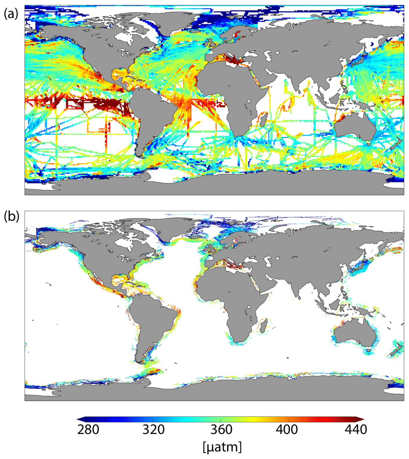
Figure 1Gridded (a) open-ocean and (b) coastal-ocean pCO2 data values extracted from the SOCATv5 database from 1998 through 2015. Each value on the maps represents the mean of all values available within each grid cell for the period considered.
Figure 2 shows the climatological mean pCO2 for both NNopen (Landschützer et al., 2016) and NNcoast (Laruelle et al., 2017). The data products rely on sea masks that lead to a common overlap area at the coastal–open-ocean transition of roughly 42×106 km2, reflecting the lack of a commonly recognized definition of the boundary between both environments. While the landward limit of the NNopen is located at 1∘ (and therefore varies in km depending on the geographical position) offshore, NNcoast extends from the coastline to either 400 km offshore or the 1000 m isobath, whichever is encountered first. The bathymetry used follows the SOCAT coastal definition (Pfeil et al., 2013) and excludes estuaries and inner water bodies (Laruelle et al., 2013, 2017). This overlap area is the subject of our error analysis described below.
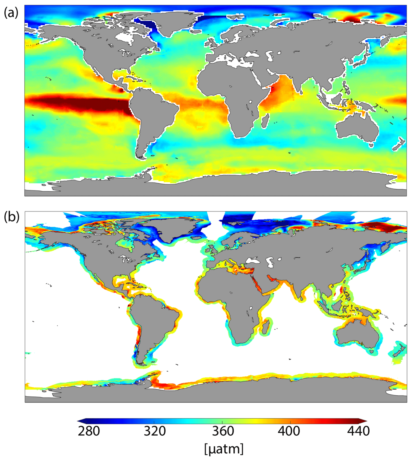
Figure 2Climatological mean of the (a) open-ocean pCO2 product by Landschützer et al. (2016) and the (b) coastal-ocean pCO2 product by Laruelle et al. (2017) for the 1998–2015 period.
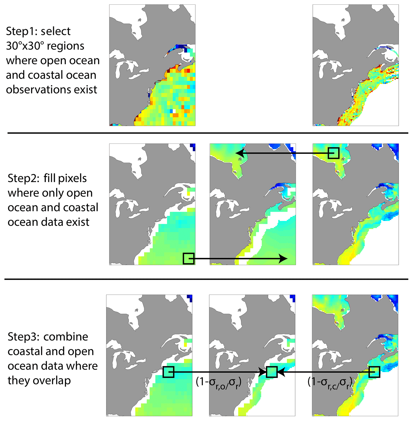
Figure 3Schematic illustration of the merging steps. Step 1 shows an illustrative example of one box that includes both coastal- and open-ocean SOCAT observations. In Step 2 empty grid cells within the box are filled with coastal ocean as well as open-ocean data points, and in Step 3 open-ocean and coastal-ocean data points are combined where both exist.
2.2 Merging algorithm
The combination of the two data products takes place in three steps, which are illustrated in Fig. 3. In a first step, we divide the globe into a raster of coarse boxes starting at 90∘ N and 180∘ W. The large box size ensures that, even in remote regions, observations from both open ocean and coastal ocean are represented in the overlap area. We then investigate the overlap area for each raster box individually. In a second step, within each box, the pixels that are only covered by either NNopen or NNcoast are assigned their respective pCO2 value. In a third step, all pixels where open-ocean and coastal-ocean pCO2 products overlap, that is, all pixels with co-located pCO2 values in the open-ocean and coastal-ocean datasets, are identified. To assign a pCO2 value in this overlap area, we weight the open and coastal pCO2 estimates by their standard error relative to the SOCATv5 open and SOCATv5 coastal-ocean datasets, respectively. We calculate the standard error at the scale of each raster, as in these larger-scale regions enough observations are available to provide an error statistic. To implement this scheme, we first calculate the standard error on each box as
where RMSE is the root mean square error of the open and coastal datasets with respect to the SOCATv5 gridded observations, N is the number of available gridded data from SOCATv5 available in a given raster box, and the subscript i refers to either NNopen or NNcoast, respectively. Since we have simply divided the open ocean from a grid into 16 equal bins, we use an effective number of for the open ocean. We do not account for autocorrelation in our calculations since we are only interested in the difference between the standard errors and assume autocorrelation lengths of similar magnitude between the SOCATv5 gridded datasets located in the coastal-ocean and open-ocean domains, respectively. Next we calculate the total error for each degree raster region r:
We also calculate the scale, for each grid cell in the overlap area, the weight given to the open-ocean and coastal-ocean local pCO2 value by the standard error of each raster region:
Substantial differences exist between the mean difference and standard deviations of NNopen and NNcoast and the respective measurements from the SOCAT database within each degree raster. Figure 4 illustrates these differences. While both NNopen and NNcoast have a near 0 bias for the mean difference, some rasters show differences exceeding 15 µatm. While more variability appears in NNcoast, this can largely be explained by the overall smaller number of gridded measurements. The larger number of gridded measurements in NNopen is a result from the division of the ∘ cells into 16 quarter degree boxes. Therefore, we reduce the number of effective degrees of freedom for the open ocean by 16. To generate the final merged product we perform an additional smoothing using a 8×8 grid point running mean filter (roughly 200 km by 200 km at the Equator).
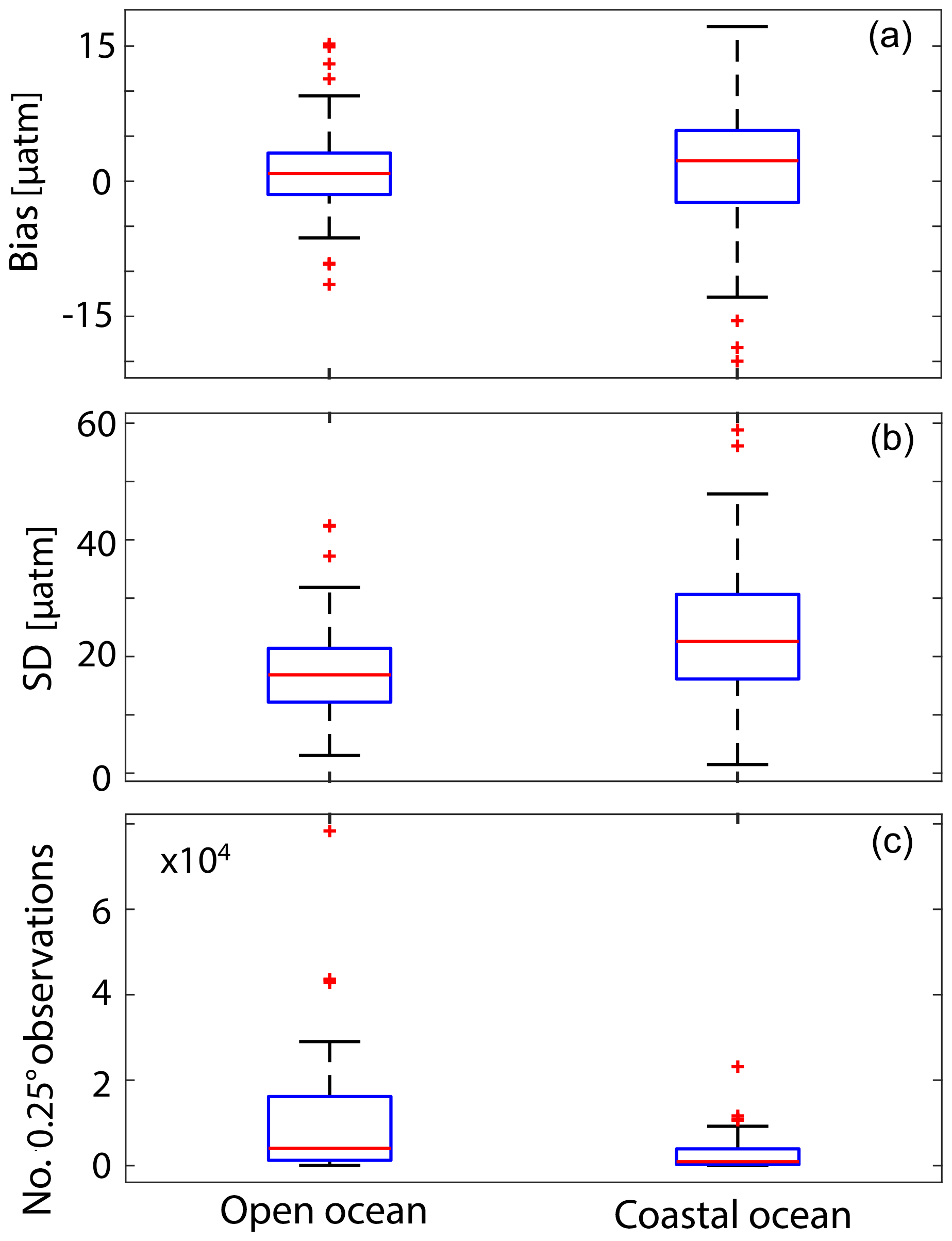
Figure 4Box-and-whisker plot of the mean difference (a), standard deviation (b) and number of 0.25∘ pixels occupied with measurements (c) in the common overlap area for each box used for merging NNopen and NNcoast.
3.1 Large-scale pCO2 patterns along the coastal–open-ocean continuum
The long term mean pCO2 field at 0.25∘ resolution for NNopen and NNcoast is shown in Fig. 5. In most oceanic regions, the transition from open to coastal ocean occurs without steep gradients, particularly in the subtropics (∼20–50∘ N) of the Northern Hemisphere. However, exceptions exist in the tropics like the Peruvian upwelling system, the Namibian–Angolan coast in the South Atlantic, and off Somalia and the Arabian Peninsula. Moreover, abrupt spatial gradients in pCO2 have been observed in large river plumes such as that of the Amazon (Ibanhez et al., 2015) or on continental shelves influenced by large rivers. The identification of such gradients, however, results only from a first order visual inspection between the two products. In what follows, we perform a quantitative analysis of the merging procedure and of the resulting pCO2 fields in the overlap area.
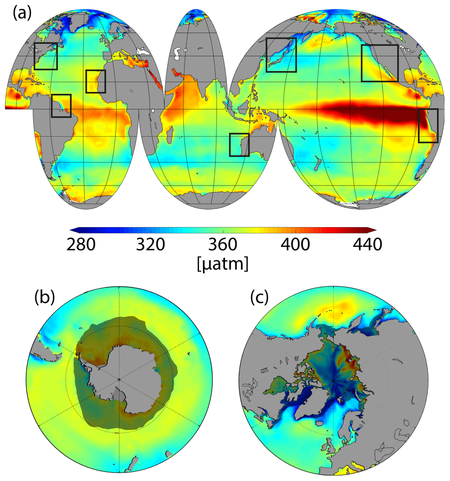
Figure 5(a) Climatological mean pCO2 of the merged product presented in this study. Panels (b) and (c) highlight the polar regions. Black boxes in (a) illustrate regions that are further investigated in the regional analysis. Shaded areas in (b) and (c) delineate the maximum sea ice extend.
Figure 6 reports the absolute pCO2 difference in % between NNcoast and NNopen along the common overlap area relative to the mean partial pressure of the merged climatology. Figure 6 shows a clear latitudinal pattern with the lowest difference in the low and subtropical latitudes and the largest differences in the high latitudes, especially in the Northern Hemisphere. We find in particular, that discrepancies are large in the newly added Arctic Ocean, but also in other seasonally ice-covered areas that have been previously described in NNopen and NNcoast publications (e.g., the Labrador Sea). One significant contributor to this difference might be that NNcoast uses information about sea ice in reconstructing the surface ocean pCO2. Acknowledging this discrepancy in seasonally ice-covered regions, we further focus our error analysis and products comparison on ice-free areas, based on the sea-ice product of Rayner et al. (2003). There are some exceptions to this general latitudinal trend consistent with our first qualitative inspection, such as along the Pacific coastline of South America, the African coast in the South Atlantic and the Arabian Sea, i.e., the regions with steep gradients already identified above. Furthermore, a gradient of decreasing pCO2 from the coast to the open ocean has been reported over the continental shelves of the eastern US and Brazil (Laruelle et al., 2015; Arruda et al., 2015) and may exist in other regions as a consequence of the influence of rivers oversaturated in CO2 combined with a limited estuarine filter (Laruelle et al., 2015). It is thus possible that the pCO2 predicted by the coastal SOM-FFN is slightly skewed towards higher values in some regions because of the presence of overall higher pCO2 observations in the calibration data pool. While there is no clear basin-wide bias structure, systematic differences can be found regionally such as in the southeastern Pacific Ocean and the Southern Ocean (south of 35∘ S). Overall, the largest relative differences are located in the overlap areas of the Arctic Ocean.
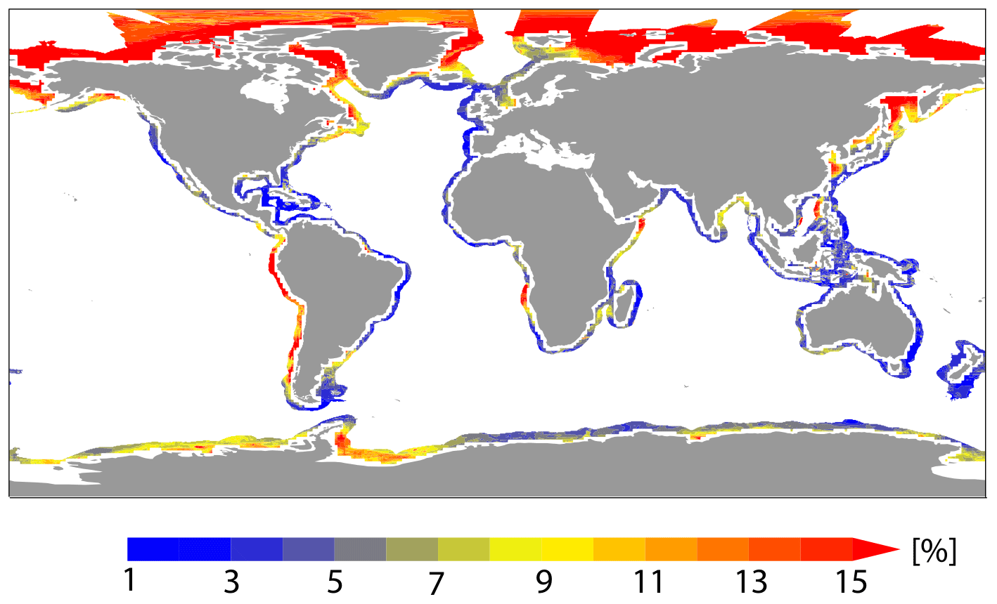
Figure 6pCO2 mismatch between NNcoast and NNopen in the overlap area relative to the mean CO2 partial pressure of the merged product. Blue colors indicate a mismatch below 5 %, whereas yellow and red colors indicate a mismatch of more than 5 %.
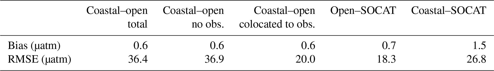
In spite of clear regional discrepancies, the mean difference, that is to say the bias, between the two estimates in the overlap area remains close to 0 µatm when integrated globally (Table 1), whether or not the comparison is limited to the locations where observations exist (Table 1 columns 1–3). Furthermore, the mismatch between the two products is in the range of the mismatch between the individual products and the available observations in SOCATv5. This result is a consequence of the neural network-based interpolation applied here at the global scale. In particular, the SOM-FFN is designed to minimize the mean squared error between available observations and the network output over the entire domain of application.
The global RMSE between NNopen and NNcoast as well as the SOCAT observations within the overlap area is in the range of previously reported global values by Landschützer et al. (2016) and Laruelle et al. (2017). In general, the spread between open-ocean and continental-coastal pCO2 varies more than the spread between coastal estimates and SOCAT or between open estimates and SOCAT, possibly indicating that the SOM-FFN method is having difficulties generalizing the pCO2 in the coastal–open-ocean continuum.
Table 1Mean error analysis (bias and RMSE) within the overlap area between NNcoast and NNopen and the observations from the SOCATv5 dataset. The comparison is performed for the total overlap area, the area fraction where no observations exist and the area covered by observations. The bias and RMSE between the pCO2 map products and the SOCATv5 open and coastal datasets are also reported.
3.2 Regional analyses of pCO2 field
A more detailed analysis is performed on the overlap of several regions selected to encompass a wide variety of conditions. These regions, indicated in Fig. 5, include three areas characterized by strong upwelling and offshore transport (Peruvian upwelling system, Canary upwelling system, US west coast) but contrasted data coverage, two data-rich regions (Sea of Japan, US east coast) of which one comprises a marginal sea (Sea of Japan), one region where seasonal data are scarce (west coast of Australia), and a region characterized by strong river outflow (Amazon river plume).
In order to further investigate the role of existing observations in upwelling regions, we first focus on the Canary upwelling system and the Peruvian upwelling system. These two regions are part of the eastern boundary upwelling systems and subject to many ecosystem stressors, such as ocean acidification or deoxygenation (Gruber, 2011). Therefore, monitoring the full aquatic continuum is essential in these regions. Both are characterized by strong upwelling and significant offshore transport of carbon-rich water from depth (see, e.g., Lovecchio et al., 2018; Franco et al., 2018) resulting in elevated pCO2 levels exceeding atmospheric levels at the sea surface. Such values are consistent with observations in the Canary upwelling system (Fig. 7) extracted from either the open-ocean SOCAT dataset (Bakker et al., 2016, Fig. 7b) or the coastal SOCAT dataset (Bakker et al., 2016, Fig. 7c) and, consequently, the merged pCO2 product (Fig. 7a). Furthermore, the Canary upwelling system is well covered by both open-ocean and coastal-ocean observations. As a consequence – despite a few areas with larger differences – the overall mismatch between the coastal ocean and NNopen (Fig. 7d) is in the range of their relative mismatch towards the observations (see Fig. 7e–f) and generally within 10 µatm.
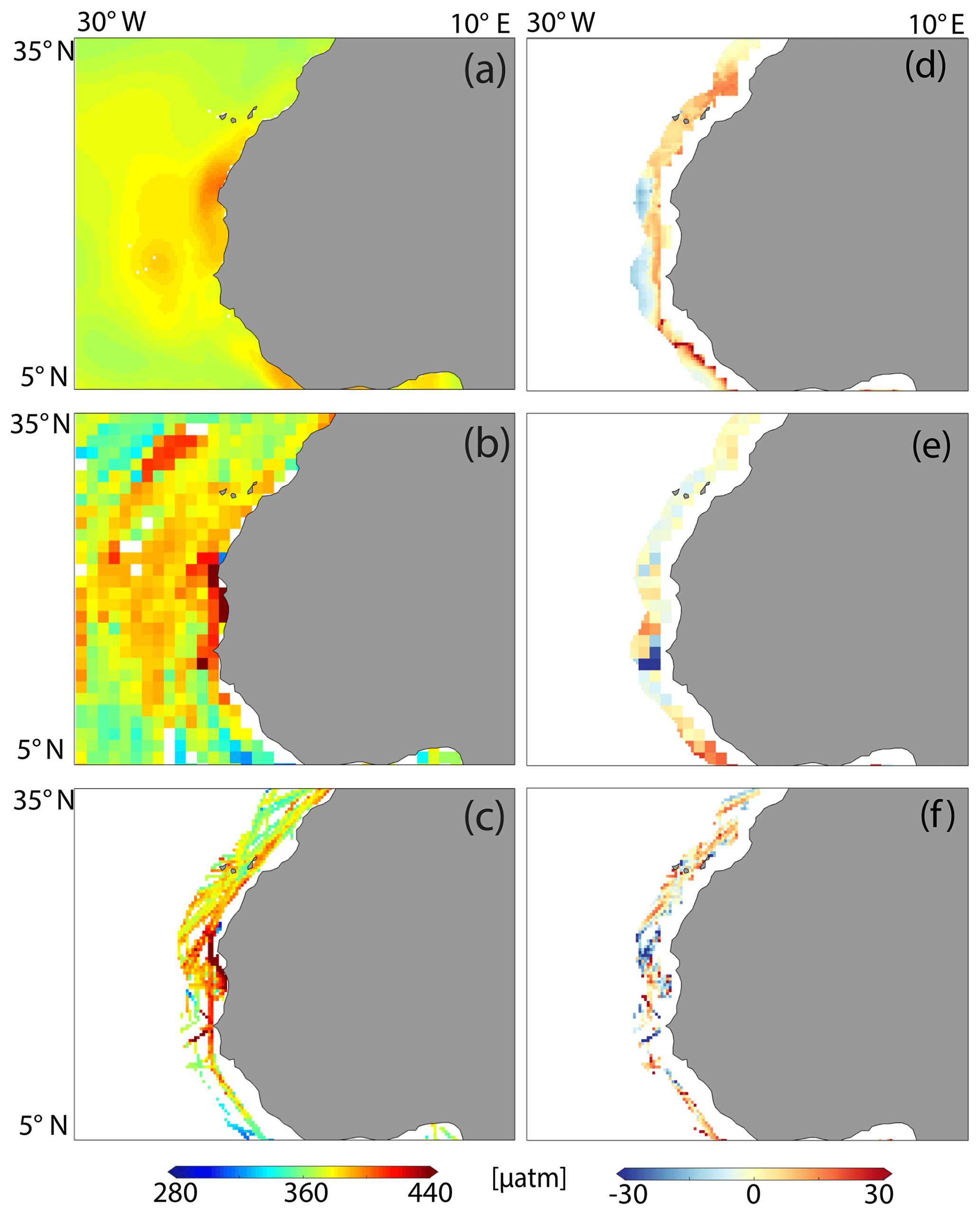
Figure 7Mismatch analysis along the Canary upwelling region for the 1998 through 2015 period. The climatological mean pCO2 is reported for (a) the merged product, (b) all available SOCATv5 data for the open ocean, and (c) all coastal SOCATv5 data (as illustrated in Fig. 1 for the global ocean). The pCO2 mismatch is illustrated in (d) as the difference between NNcoast and NNopen. Panel (e) reports the mismatch between the NNopen and the SOCATv5 open-ocean dataset along the overlap area, while panel (f) reports the mismatch between the coastal product and the SOCATv5 coastal dataset along the overlap area.
In contrast to the Canary upwelling system, the Peruvian upwelling system shows a steep pCO2 gradient between the offshore and nearshore regions (Fig. 8a), particularly just south of the Equator. A closer inspection of the available observations (Fig. 8b and c) reveals that, particularly in the nearshore domain at the Equator, several of the few available observations of the sea surface pCO2 indicate low partial pressures resulting in a low reconstructed coastal pCO2, as already identified by Laruelle et al. (2017). The mismatch that results from the upscaling of the low pCO2 data in the coastal domain is further reflected in the difference between the coastal- and open-ocean pCO2 fields in the overlap area (Fig. 8d). The mismatch between the open ocean and NNcoast exceeds 30 µatm and is larger than the difference between the individual products and the observations (Fig. 8e–f), suggesting that the disagreement between the open ocean and NNcoast in the overlap area stems from their data treatment. The fewer existing coastal observations of low pCO2 are extrapolated in space, spreading a potential mismatch over a larger area. Likewise, the nearshore domain in the NNopen is influenced by the high CO2 partial pressures offshore. This data sparsity and spatial heterogeneity is a further challenge for model evaluation (Franco et al., 2018).
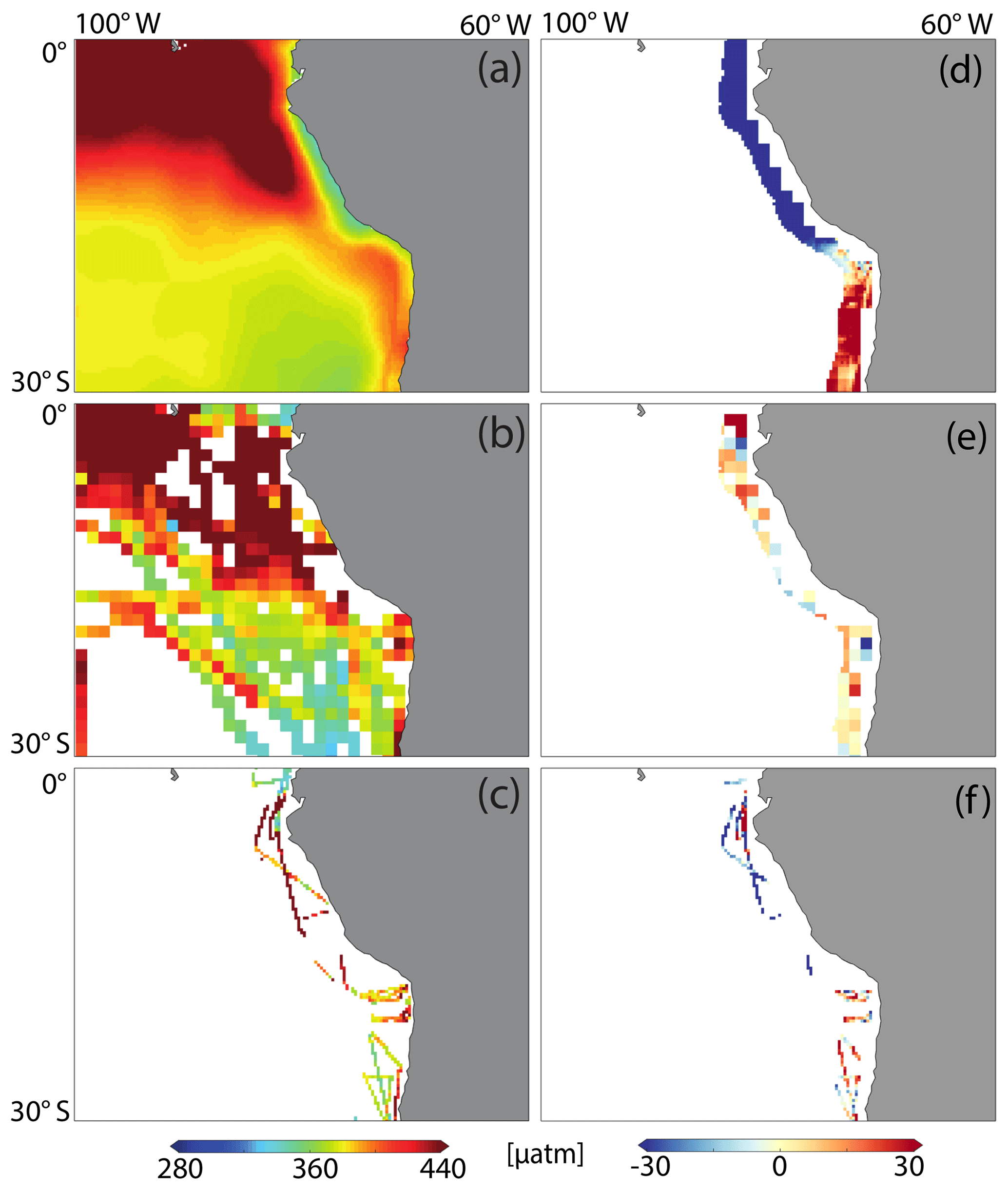
Figure 8Mismatch analysis along the Peruvian upwelling region for the 1998 through 2015 period. The climatological mean pCO2 is reported for (a) the merged product, (b) all available SOCATv5 data for the open ocean, and (c) all coastal SOCATv5 data (as illustrated in Fig. 1 for the global ocean). The pCO2 mismatch is illustrated in (d) as the difference between NNcoast and NNopen. Panel (e) reports the mismatch between the NNopen and the SOCATv5 open-ocean dataset along the overlap area, while panel (f) reports the mismatch between the coastal product and the SOCATv5 coastal dataset along the overlap area.
No steep pCO2 gradient can be identified along the west coast of Australia in the merged product (Fig. 9). The highest CO2 partial pressures are found nearshore along the Leeuwin current (Smith et al., 1991), and the lowest observed pCO2 can be found along the West Australian Current. The area is spatially covered both in the open- and coastal-ocean SOCAT datasets (Fig. 9b and c), and therefore the overall difference towards observed values remains among the smallest of all investigated regions. This is remarkable given the lack of seasonal observations, which will be discussed in the subsequent section. NNopen and NNcoast agree with each other spatially within 15 µatm (Fig. 9d), which is in the range of the mismatch between the individual products and the respective SOCAT observations (Fig. 9e–f). Both products tend to overestimate the low pCO2 towards the south of the domain. This is reflected in the positive mismatch towards the SOCAT observations (Fig. 9e and f) in the common overlap area where, the difference between the neural network estimates and the raw data exceeds 15 µatm for both products.
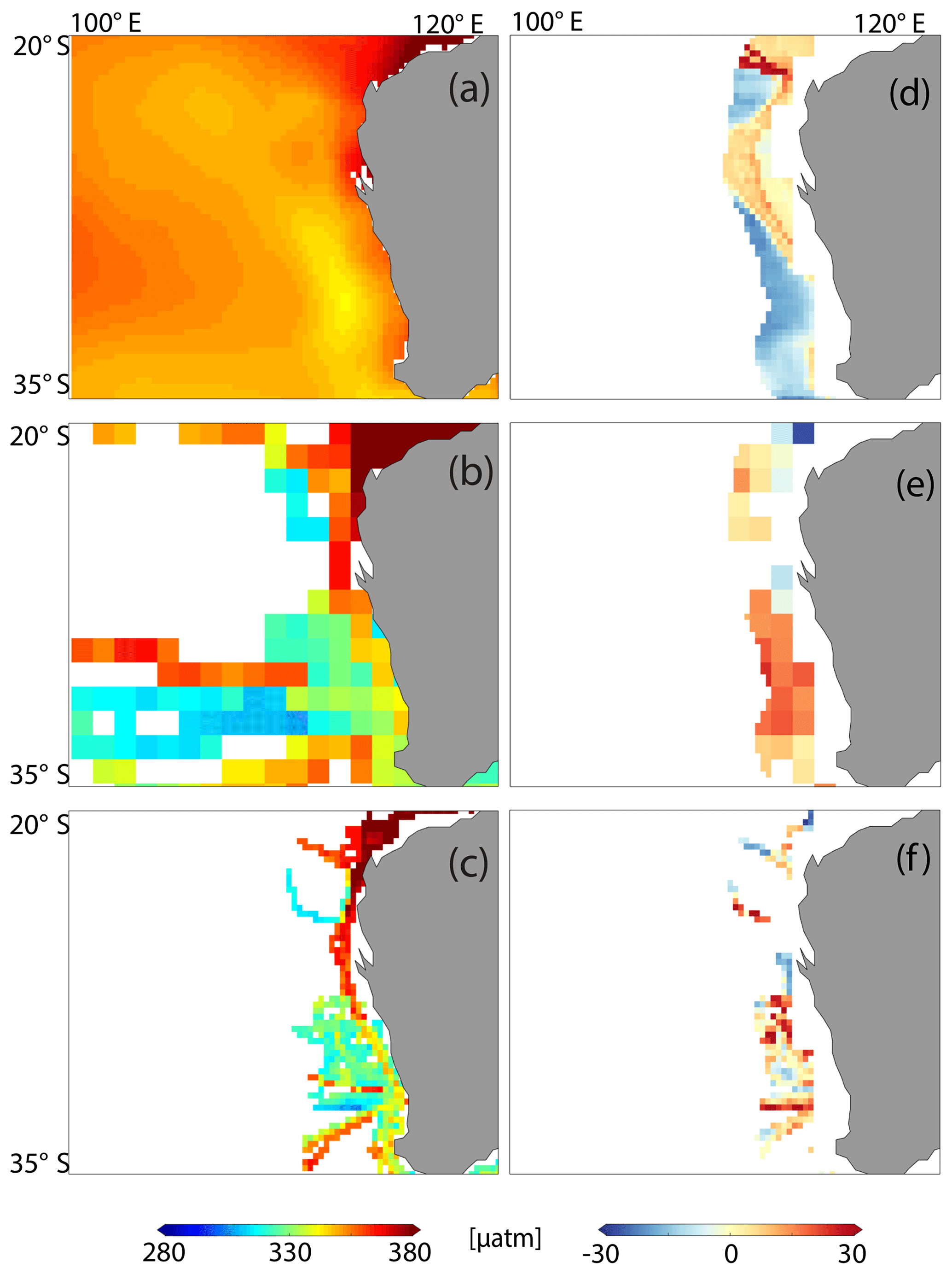
Figure 9Mismatch analysis along the Australian west coast region for the 1998 through 2015 period. The climatological mean pCO2 is reported for (a) the merged product, (b) all available SOCATv5 data for the open ocean, and (c) all coastal SOCATv5 data (as illustrated in Fig. 1 for the global ocean). The pCO2 mismatch is illustrated in (d) as the difference between NNcoast and NNopen. Panel (e) reports the mismatch between the NNopen and the SOCATv5 open-ocean dataset along the overlap area, while panel (f) reports the mismatch between the coastal product and the SOCATv5 coastal dataset along the overlap area.
Observations in the Sea of Japan and adjacent Pacific Ocean suggest large variability in the pCO2 with the lowest observed values just north of the Korean Peninsula and the highest observed pCO2 in the Yellow Sea (Fig. 10b–c). Furthermore, low pCO2 is also observed south of the island of Hokkaido. These large spatial variations in the pCO2 are also visible in the merged pCO2 product (Fig. 10a). A notable exception is the Korean Straight, where observations suggest a lower pCO2 than reconstructed. The strong variability in the observed pCO2 reflects the complex carbon dynamics in the Sea of Japan (Chen et al., 1995; Park et al., 2006), which is also reflected in the larger mismatch between products and towards the SOCAT observations (Fig. 10d–f). The disagreement may indicate that the global-scale NNopen and NNcoast products are not particularly skilled in representing the strong regional dynamics of marginal sea. A better agreement between the neural network reconstructions and observations is found in the Pacific Ocean east of the Japanese islands, where the merged estimate also reveals a better agreement between NNopen and NNcoast (Fig. 10d) and low biases in the range of 5 µatm towards SOCAT observations (Fig. 10e and f).

Figure 10Mismatch analysis along the Sea of Japan region for the 1998 through 2015 period. The climatological mean pCO2 is reported for (a) the merged product, (b) all available SOCATv5 data for the open ocean, and (c) all coastal SOCATv5 data (as illustrated in Fig. 1 for the global ocean). The pCO2 mismatch is illustrated in (d) as the difference between NNcoast and NNopen. Panel (e) reports the mismatch between the NNopen and the SOCATv5 open-ocean dataset along the overlap area, while panel (f) reports the mismatch between the coastal product and the SOCATv5 coastal dataset along the overlap area.
Some of the best monitored regions spanning both coastal and nearshore open ocean can be found along the US coast (Fennel et al., 2008; Signorini et al., 2013; Laruelle et al., 2015; Fennel et al., 2019). Indeed all open ocean and almost all coastal pixels are filled with raw observations off the eastern US coastline. While the mean of all observed pCO2 values from SOCAT (Fig. 11b and c) suggests substantial regional variability, the merged estimate (Fig. 11a) is, as a result of the neural network interpolation algorithm, substantially smoother. In particular, the lower latitudes (25–35∘ N, Fig. 11e and f) are well reconstructed by the neural network algorithms in both open- and coastal-ocean domains. Larger discrepancies however exist in the higher latitudes (35–45∘ N, Fig. 11e and f). Landschützer et al. (2014) attributed a larger mismatch to the complex biogeochemical dynamics of the Gulf Stream region, where the measured pCO2 is underestimated by both the open and coastal products. The strong mesoscale dynamics and the influence of the cold Labrador current in this region are not well represented in the rather coarse 0.25∘ NNcoast and 1∘ NNopen products. The smooth transition between coastal and open ocean in Fig. 11a indeed suggests that the intensively surveyed US east coast aquatic continuum can be well reconstructed by combining the open-ocean and coastal-ocean pCO2 datasets.
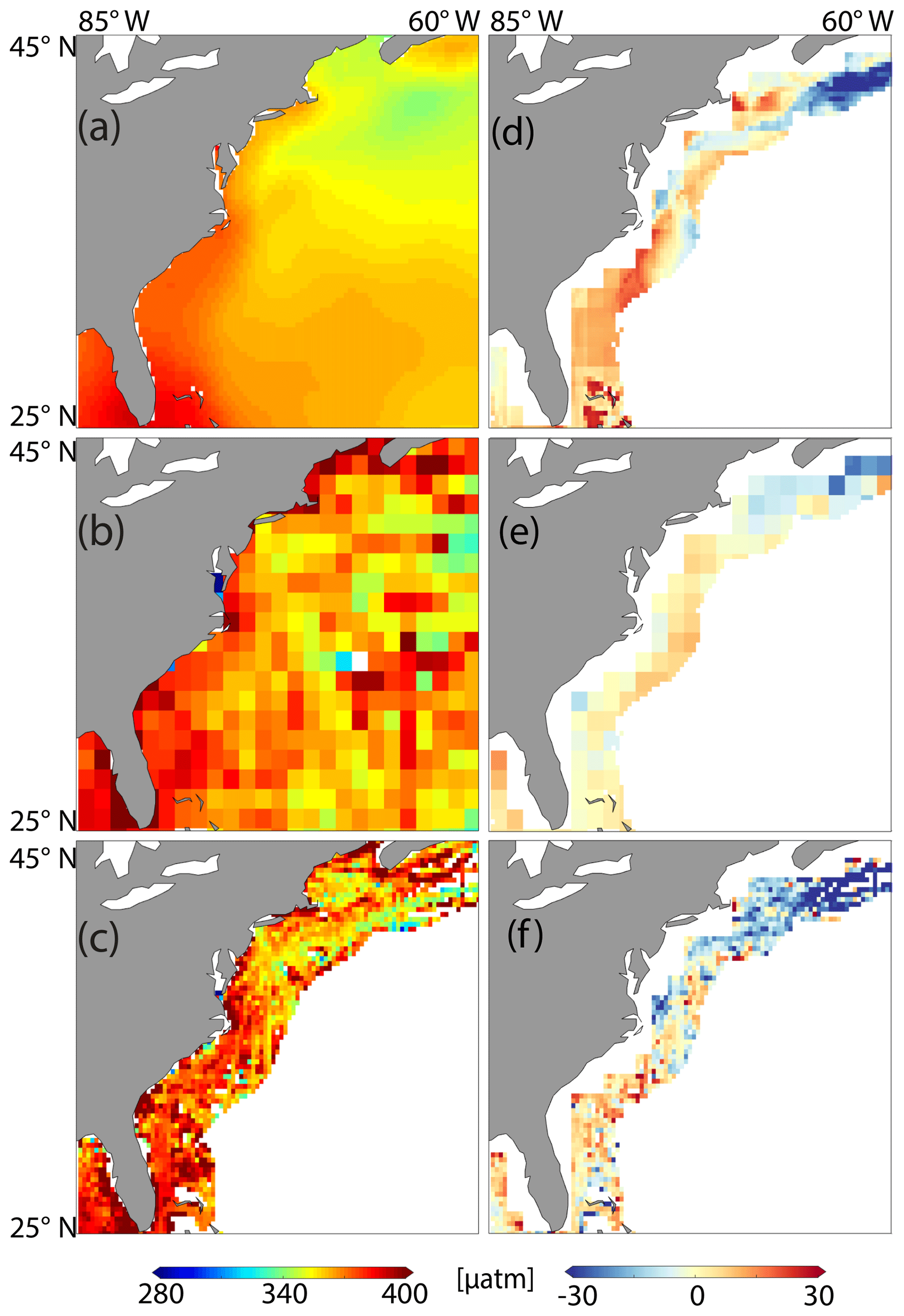
Figure 11Mismatch analysis along the United States east coast for the 1998 through 2015 period. The climatological mean pCO2 is reported for (a) the merged product, (b) all available SOCATv5 data for the open ocean, and (c) all coastal SOCATv5 data (as illustrated in Fig. 1 for the global ocean). The pCO2 mismatch is illustrated in (d) as the difference between NNcoast and NNopen. Panel (e) reports the mismatch between the NNopen and the SOCATv5 open-ocean dataset along the overlap area, while panel (f) reports the mismatch between the coastal product and the SOCATv5 coastal dataset along the overlap area.
Similarly well monitored to the US east coast is the US west coast upwelling system, not the least because its variability is tightly linked to El Niño–Southern Oscillation (ENSO) (see, e.g., Lynn and Bograd, 2002; Frischknecht et al., 2015). Here, we find an overall good agreement between NNcoast and NNopen. The agreement in the overlap area of the merged product (Fig. 12d) is among the best reported globally. Interestingly, nearshore, the merged estimate (Fig. 12a) reveals a lower mean pCO2 than suggested from both the open-ocean and coastal-ocean SOCAT datasets (Fig. 12b and c). The small error compared to the SOCAT observations suggests that this is not the result of the two products being in disagreement but might relate to changes in upwelling as a result of interannual variability linked to ENSO events that are not well captured by the merged product.
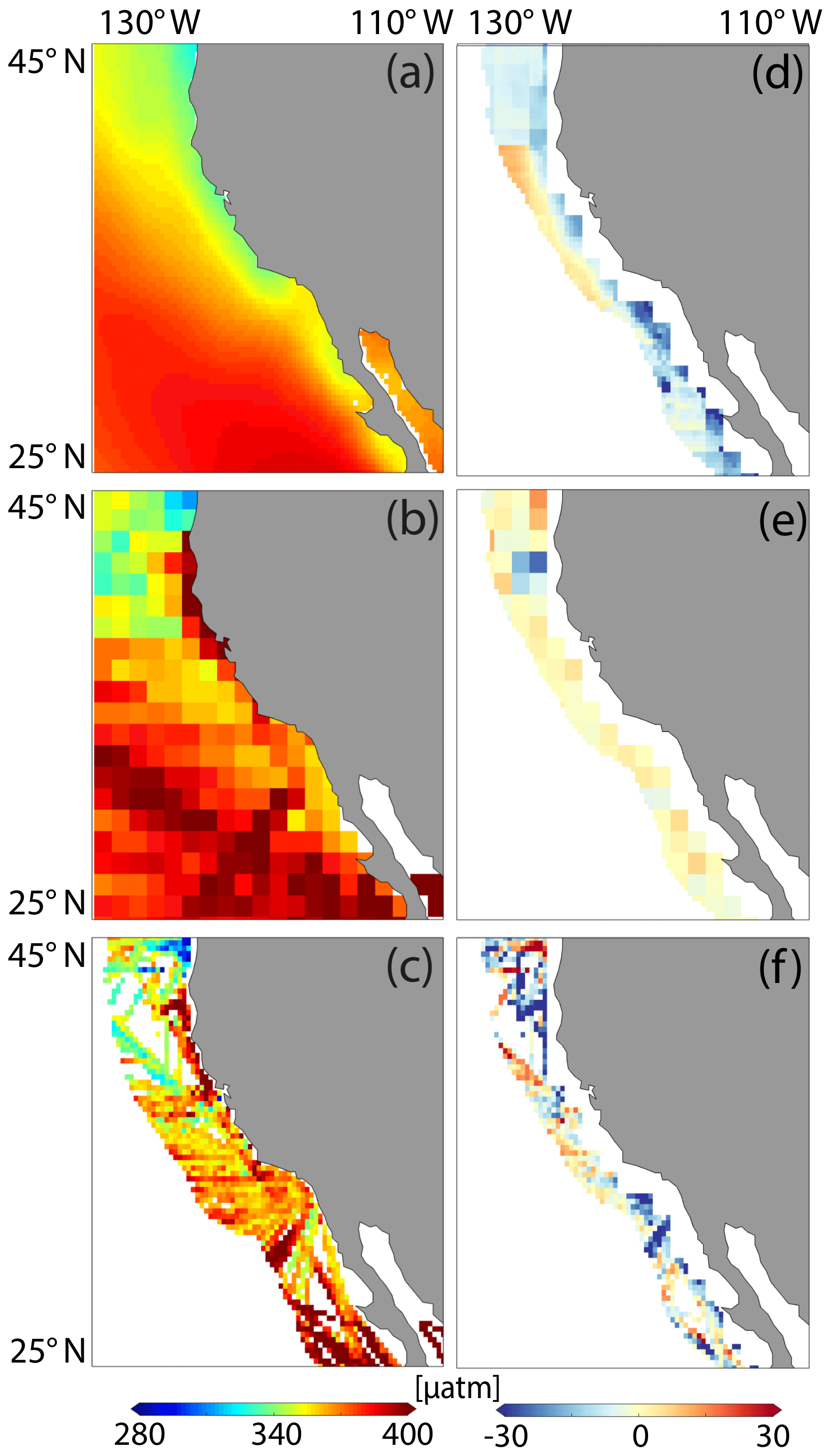
Figure 12Mismatch analysis along the United States west coast for the 1998 through 2015 period. The climatological mean pCO2 is reported for (a) the merged product, (b) all available SOCATv5 data for the open ocean, and (c) all coastal SOCATv5 data (as illustrated in Fig. 1 for the global ocean). The pCO2 mismatch is illustrated in (d) as the difference between NNcoast and NNopen. Panel (e) reports the mismatch between the NNopen and the SOCATv5 open-ocean dataset along the overlap area, while panel (f) reports the mismatch between the coastal product and the SOCATv5 coastal dataset along the overlap area.
Finally, we investigate the spatial structure of the reconstructed pCO2 from a region typically dominated by the freshwater outflow of a large river mouth, i.e., the Amazon outflow in the tropical Atlantic Ocean (Fig. 13). Studies linking circulation with the local CO2 dynamics are sparse (Ibanhez et al., 2015; Lefevre et al., 2013). Very few observations exist, particularly in the nearshore region (Fig. 13b–c). Nevertheless, studies suggest that the Amazon river outflow becomes a significant CO2 sink when it mixes with ocean waters (Lefevre et al., 2010). The strong variance in observed pCO2 (Bakker et al., 2016) provides a challenge for any algorithm to reconstruct the full pCO2 field in such a region. Nevertheless, both coastal and oceanic data products are in good agreement (Fig. 13d) with the exception of the area under direct influence of Amazon river outflow. This difference potentially stems from the NNopen being unable to associate the pCO2 variability observed in this area with the strong salinity gradients, which is better represented in the coastal-ocean pCO2 product. Both products show differences of similar magnitude when compared to the SOCAT observations (Fig. 13e–f) and similar error structures as both products overestimate the pCO2 in the northern and underestimate the pCO2 in the southern sections of the overlap area.

Figure 13Mismatch analysis along the Amazon outflow region for the 1998 through 2015 period. The climatological mean pCO2 is reported for (a) the merged product, (b) all available SOCATv5 data for the open ocean, and (c) all coastal SOCATv5 data (as illustrated in Fig. 1 for the global ocean). The pCO2 mismatch is illustrated in (d) as the difference between NNcoast and NNopen. Panel (e) reports the mismatch between the NNopen and the SOCATv5 open-ocean dataset along the overlap area, while panel (f) reports the mismatch between the coastal product and the SOCATv5 coastal dataset along the overlap area.
While global errors between the data products and observations remain low (see Table 1), Figs. 7–13 show that, at the regional scale, larger differences emerge. We therefore expend our standard error statistics as presented in Table 2 for the selected regions. Overall, we find at the regional level that the inter-product mismatch, represented by the bias, is substantially larger than in the global analysis but does not exceed ∼8 µatm with one prominent exception: the Peruvian upwelling system where the mismatch reaches 14.8 µatm. Here, the substantial disagreement between the two products results from the underestimation of the coastal observations in the overlap domain by the coastal-ocean pCO2 product already shown by Laruelle et al. (2017).
Table 2Mean error analysis (bias and RMSE) within the overlap area between NNopen and NNcoast and the observations from the SOCATv5 dataset (Bakker et al., 2016) for 7 oceanic regions. The comparison is performed for the total overlap area, the area fraction where no observations exist and the area covered by observations. The biases and RMSE between pCO2 products and SOCATv5 datasets are also reported for the open ocean and coastal ocean.
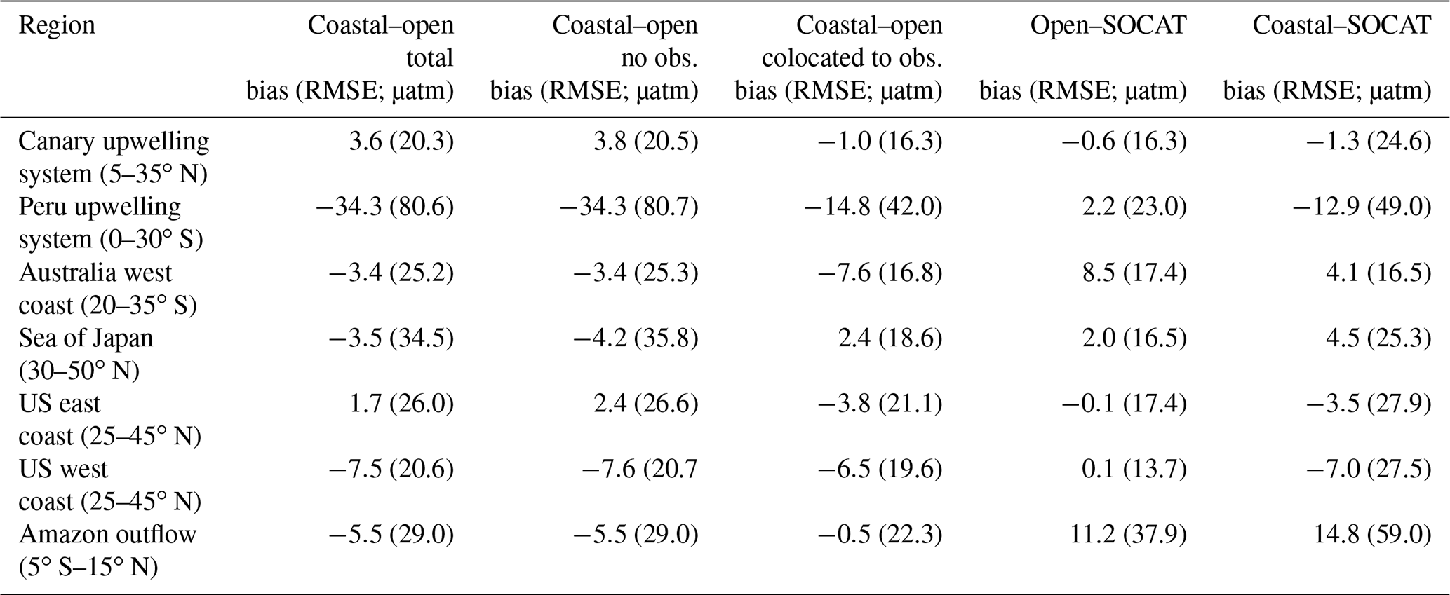
We find that the bias between NNopen and NNcoast in the overlap area is larger where they are not co-located to observations (Table 2). The error spread between NNopen and NNcoast, represented by the RMSE, is likewise larger in areas where fewer observations exist (contrast column 1 and 2 in Table 2). Exceptions include the US east coast and the west coast of Australia possibly linked to the larger mismatch of the individual products towards the respective SOCAT observations at these locations. Results from both products in the Amazon outflow region, in the US east coast for NNcoast and in the west coast of Australia for NNopen, show a larger bias towards the SOCAT observations than the respective inter-model bias, illustrating that both methods generalize well. This further suggests that the estimates are locally constrained by information outside the investigated domain, which is possible considering the spatial distributions of the biogeochemical provinces generated by the SOM.
3.3 Seasonality
A further analysis in the selected regions aims to investigate the seasonal differences in pCO2 between the original data products, the merged product and observations (Fig. 14). In particular, we investigate the extent to which the mean biases reported above can be explained by seasonal differences in pCO2 among the different products. To this end, we average all months from 1998 through 2015 to create a seasonal climatology from our pCO2 products, without correction to a nominal reference year. We repeat this procedure for the SOCAT datasets, likewise without any corrections but being aware that this could lead to a sampling bias in the observed climatology. This approach is justified because we lack knowledge about the short-term variability in the observed carbon cycle, and it is thus unclear on how such a correction would improve the representation of the observed pCO2 field.
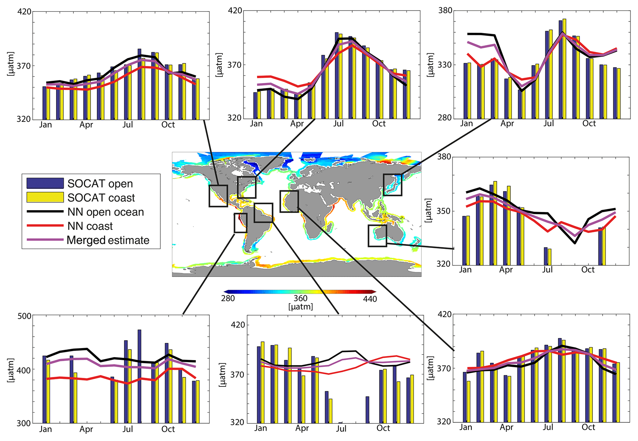
Figure 14Seasonal pCO2 cycle for the seven regions discussed in the text and highlighted in the center map. The seasonal cycles include a comparison of the monthly mean SOCAT observations without any interpolation (blue and yellow bars) as well as the open-ocean (blue line), coastal-ocean (red line) and merged (magenta line) reconstructions based on the respective SOCAT observations.
In spite of the lack of seasonal sampling bias corrections, our analysis displays, for most regions, a close correspondence within a few microatmospheres (µatm) between open-ocean and coastal-ocean pCO2 data from SOCAT within the overlap area (blues and yellow bars in Fig. 14) with deviations mostly arising in the Peruvian upwelling system and the Amazon outflow regions where monthly differences can exceed 10 µatm. The good correspondence is expected to some degree because both datasets share a large fraction of the data. The analysis shows that the seasonality of the neural network-based on NNopen and NNcoast satisfactorily reproduces the seasonal fluctuations obtained directly from the raw data, highlighting that the reconstructed seasonal cycle is well constrained by the existing observations. Monthly deviations between the products largely stay within 10 µatm. An exception is the Sea of Japan in boreal winter, where NNopen overestimates the surface ocean pCO2 values recorded in the SOCAT data. All but three of the selected regions have full seasonal data coverage. The three regions without full coverage are the west coast of Australia, the Amazon outflow region and the Peruvian upwelling system. Despite the lack of seasonal observations along the west coast of Australia, both products agree well with regards to the seasonal cycle and differences stay within of 8–10 µatm between the different products. Likewise, the otherwise good agreement between coastal-ocean and open-ocean estimate breaks down in the boreal summer in the Amazon outflow region, despite the lack of strong seasonality in the tropical latitudes.
The largest mismatch between data products and observations exists along the Peruvian upwelling system, where monthly differences between open-ocean and coastal-ocean estimates exceed 40 µatm. Both estimates however show similar seasonal variability. The seasonal analysis further reveals that from all investigated regions, the Peruvian upwelling system shows the largest monthly differences between open-ocean and coastal-ocean SOCAT observations, with, for example, mean differences in March exceeding 30 µatm between the open-ocean and coastal-ocean SOCAT datasets (Bakker et al., 2016). Furthermore, the largest observed partial pressures in NNopen appear in August where no data are available in the coastal-ocean SOCAT dataset, highlighting that NNopen draws information from observations further away from shore during this month.
The merged climatology (Landschützer et al., 2020a, https://doi.org/10.25921/qb25-f418) is available from NCEI OCADS and can be accessed via https://www.nodc.noaa.gov/ocads/oceans/MPI-ULB-SOM_FFN_clim.html (last access: 8 April 2020) (Landschützer et al., 2020b, https://doi.org/10.25921/qb25-f418). NNopen is available via NCEI OCADS and is accessible online: https://www.nodc.noaa.gov/ocads/oceans/SPCO2_1982_present_ETH_SOM_FFN.html (last access: 10 July 2020) (Landschützer et al., 2020b, https://doi.org/10.7289/V5Z899N6). The NNcoast description and dataset can be downloaded from Laruelle et al. (2017).
In this analysis, we combined two recently published sea surface pCO2 products, covering the open-ocean and the coastal-ocean domain. While the spatial coverage of NNopen includes all surface waters located further than 1∘ off the coast, the spatial coverage of the NNcoast includes surface waters until 400 km off the coast, leading to an overlap domain of roughly 300 km close to the Equator and increasing in extend towards the poles around the land surface. The common overlap area was used to compare both reconstructed pCO2 estimates at regional to global scale and whether the observed agreement/disagreement is linked to data availability.
Our results show that, for most of the global ocean and particularly the subtropical latitudes in the Northern Hemisphere, NNopen and NNcoast agree well within the overlap domain. However, stronger differences exist in other parts of the world, particularly in the Peruvian upwelling system, the Arctic and Antarctic, the African coastline in the South Atlantic and the Arabian Sea, where fewer observations exist. Additionally, we find larger discrepancies in the marginal Sea of Japan. In other regions without complete seasonal data coverage such as the west coast of Australia, however, both products compare well. We therefore conclude that the lack of data coverage and the biogeochemical complexity triggered by upwelling, river influx or seasonal ice coverage both contribute to the mismatch. Additionally, methodological differences between NNopen and NNcoast, such as differences in predictor data, result in local differences, for example, in ice-covered regions where NNcoast relies on sea ice as predictor or shallow, stratified waters, where mixed layer depth serves as an important proxy in NNopen. Closer inspection reveals that for most of the overlap regions, the difference between the open-ocean and coastal-ocean estimates falls within the range of the difference between NNopen and NNcoast and the respective SOCAT dataset from which they were created. Therefore, the combined pCO2 climatology is not only a step forward in including the full oceanic domain with all its complexity into carbon budget analyses, but it also helps to identify areas where additional continuous observations are critically needed to close current knowledge gaps.
Another way forward to further reduce the bias between the coastal- and open-ocean estimates would be to reconsider the cut-off definition between the two domains. Data-sparse and often strongly variable regions such as the Peruvian upwelling system are very sensitive to the data selected to generate the pCO2 fields. The overlap analysis proposed here, particularly the percent mismatch and RMSE analysis, further serves as a benchmark on how well we understand the coastal-to-open ocean continuum and its spatial variability and where we still lack essential measurements to close the gap between existing estimates, for example, the Peruvian upwelling system or the seasonally ice-covered high-latitude regions, in particular the Arctic Ocean. A next step should include the reduction of the mismatch between coastal- and open-ocean estimates in order to combine the two. This is an essential step towards an observation-driven global carbon budget. Closing such a gap, however, requires close collaborations between open-ocean and coastal-ocean carbon cycle scientists in the future to be considered of high importance.
Finally, we introduced a new concept where we can locally evaluate the upscaling of existing measurements based on a common overlap region. In this study, we focused on mean differences and seasonal climatologies at regional and global scales. We find an encouraging agreement between seasonal cycles which gives us confidence that the existing products might be suitable to be applied to study lower frequency signals such as trends and interannual variability. Understanding of how differences in trends and inter-annual variabilities between the coastal and open oceans emerge and how they are linked to data availability should be a next step. Such an analysis is essential to gain confidence in observational constraints and to find ways to further improve them in order to close the global carbon budget based on observations and provide data products form model benchmarking. Our approach can also be used to compare other overlapping datasets at a time when advanced interpolation techniques are yielding more and more oceanic data products with different spatial extensions and boundaries. Our study is therefore an important step towards a truly representative global ocean observation-based CO2 product that includes all ocean domains.
PL designed the study and wrote the manuscript together with PR, GGL and AR. PL developed the open-ocean pCO2 product and GGL developed the coastal-ocean pCO2 product.
The authors declare that they have no conflict of interest.
Peter Landschützer is supported by the Max Planck Society for the Advancement of Science. The research leading to these results has received funding from the European Community's Horizon 2020 project under grant agreement no. 821003 (4C). Goulven G. Laruelle is a research associate of the F.R.S-FNRS at the Université Libre de Bruxelles. Pierre Regnier received funding from the VERIFY project from the European Union Horizon 2020 research and innovation program under grant agreement no. 776810. This study benefited from discussions with Katharina Six from the Max Planck Institute for Meteorology. The Surface Ocean CO2 Atlas (SOCAT) is an international effort, supported by the International Ocean Carbon Coordination Project (IOCCP), the Surface Ocean Lower Atmosphere Study (SOLAS), and the Integrated Marine Biogeochemistry and Ecosystem Research program (IMBER), to deliver a uniformly quality-controlled surface ocean CO2 database. The many researchers and funding agencies responsible for the collection of data and quality control are thanked for their contributions to SOCAT.
This research has been supported by the European Commission projects 4C (grant no. 821003) and VERIFY (grant no. 776810).
This paper was edited by Jens Klump and reviewed by Rik Wanninkhof and one anonymous referee.
Arruda, R., Calil, P. H. R., Bianchi, A. A., Doney, S. C., Gruber, N., Lima, I., and Turi, G.: Air-sea CO2 fluxes and the controls on ocean surface pCO2 seasonal variability in the coastal and open-ocean southwestern Atlantic Ocean: a modeling study, Biogeosciences, 12, 5793–5809, https://doi.org/10.5194/bg-12-5793-2015, 2015. a
Bakker, D. C. E., Pfeil, B., Smith, K., Hankin, S., Olsen, A., Alin, S. R., Cosca, C., Harasawa, S., Kozyr, A., Nojiri, Y., O'Brien, K. M., Schuster, U., Telszewski, M., Tilbrook, B., Wada, C., Akl, J., Barbero, L., Bates, N. R., Boutin, J., Bozec, Y., Cai, W.-J., Castle, R. D., Chavez, F. P., Chen, L., Chierici, M., Currie, K., de Baar, H. J. W., Evans, W., Feely, R. A., Fransson, A., Gao, Z., Hales, B., Hardman-Mountford, N. J., Hoppema, M., Huang, W.-J., Hunt, C. W., Huss, B., Ichikawa, T., Johannessen, T., Jones, E. M., Jones, S. D., Jutterström, S., Kitidis, V., Körtzinger, A., Landschützer, P., Lauvset, S. K., Lefèvre, N., Manke, A. B., Mathis, J. T., Merlivat, L., Metzl, N., Murata, A., Newberger, T., Omar, A. M., Ono, T., Park, G.-H., Paterson, K., Pierrot, D., Ríos, A. F., Sabine, C. L., Saito, S., Salisbury, J., Sarma, V. V. S. S., Schlitzer, R., Sieger, R., Skjelvan, I., Steinhoff, T., Sullivan, K. F., Sun, H., Sutton, A. J., Suzuki, T., Sweeney, C., Takahashi, T., Tjiputra, J., Tsurushima, N., van Heuven, S. M. A. C., Vandemark, D., Vlahos, P., Wallace, D. W. R., Wanninkhof, R., and Watson, A. J.: An update to the Surface Ocean CO2 Atlas (SOCAT version 2), Earth Syst. Sci. Data, 6, 69–90, https://doi.org/10.5194/essd-6-69-2014, 2014. a
Bakker, D. C. E., Pfeil, B., Landa, C. S., Metzl, N., O'Brien, K. M., Olsen, A., Smith, K., Cosca, C., Harasawa, S., Jones, S. D., Nakaoka, S., Nojiri, Y., Schuster, U., Steinhoff, T., Sweeney, C., Takahashi, T., Tilbrook, B., Wada, C., Wanninkhof, R., Alin, S. R., Balestrini, C. F., Barbero, L., Bates, N. R., Bianchi, A. A., Bonou, F., Boutin, J., Bozec, Y., Burger, E. F., Cai, W.-J., Castle, R. D., Chen, L., Chierici, M., Currie, K., Evans, W., Featherstone, C., Feely, R. A., Fransson, A., Goyet, C., Greenwood, N., Gregor, L., Hankin, S., Hardman-Mountford, N. J., Harlay, J., Hauck, J., Hoppema, M., Humphreys, M. P., Hunt, C. W., Huss, B., Ibánhez, J. S. P., Johannessen, T., Keeling, R., Kitidis, V., Körtzinger, A., Kozyr, A., Krasakopoulou, E., Kuwata, A., Landschützer, P., Lauvset, S. K., Lefèvre, N., Lo Monaco, C., Manke, A., Mathis, J. T., Merlivat, L., Millero, F. J., Monteiro, P. M. S., Munro, D. R., Murata, A., Newberger, T., Omar, A. M., Ono, T., Paterson, K., Pearce, D., Pierrot, D., Robbins, L. L., Saito, S., Salisbury, J., Schlitzer, R., Schneider, B., Schweitzer, R., Sieger, R., Skjelvan, I., Sullivan, K. F., Sutherland, S. C., Sutton, A. J., Tadokoro, K., Telszewski, M., Tuma, M., van Heuven, S. M. A. C., Vandemark, D., Ward, B., Watson, A. J., and Xu, S.: A multi-decade record of high-quality fCO2 data in version 3 of the Surface Ocean CO2 Atlas (SOCAT), Earth Syst. Sci. Data, 8, 383–413, https://doi.org/10.5194/essd-8-383-2016, 2016. a, b, c, d, e, f, g
Borges, A. V., Delille, B., and Frankignoulle, M.: Budgeting sinks and sources of CO2 in the coastal ocean: Diversity of ecosystems counts, Geophys. Res. Lett., 32, L14601, https://doi.org/10.1029/2005GL023053, 2005. a, b, c
Cai, W. J.: Estuarine and coastal ocean carbon paradox: CO2 sinks or sites of terrestrial carbon incineration?, Annu. Rev. Mar. Sci., 3, 123–145, 2011. a, b
Cai, W.-J., Dai, M. H., Wang, Y. C.: Air sea exchange of carbon dioxide in ocean margins: A province based synthesis, Geophys. Res. Lett., 33, L12603, https://doi.org/10.1029/2006GL026219, 2006. a
Chen, C. T. A. and Borges, A. V.: Reconciling opposing views on carbon cycling in the coastal ocean: continental shelves as sinks and near-shore ecosystems as sources of atmospheric CO2, Deep-Sea Res. Pt. II, 56, 578–590, 2009. a
Chen, C.-T. A., Wang, S.-L., and Bychkov, A. S.: Carbonate chemistry of the Sea of Japan, J. Geophys. Res.-Oceans, 100, 13737–13745, https://doi.org/10.1029/95JC00939, 1995. a
Chen, C.-T. A., Huang, T.-H., Chen, Y.-C., Bai, Y., He, X., and Kang, Y.: Air–sea exchanges of CO2 in the world's coastal seas, Biogeosciences, 10, 6509–6544, https://doi.org/10.5194/bg-10-6509-2013, 2013. a
Dai, M., Cao, Z., Guo, X., Zhai, W., Liu, Z., Yin, Z., Xu, Y., Gan, J., Hu, J., and Du, C.: Why are some marginal seas sources of atmospheric CO2?, Geophys. Res. Lett., 40, 2154–2158, https://doi.org/10.1002/grl.50390, 2013. a
de Boyer Montegut, C., Madec, G., Fischer, A. S., Lazar, A., and Iudicone, D.: Mixed layer depth over the global ocean: An examination of profile data and a profile-based climatology, J. Geophys. Res., 109, C12003, https://doi.org/10.1029/2004JC002378, 2004. a
Fennel, K., Wilkin, J., Previdi, M., and Najjar, R.: Denitrification effects on air-sea CO2 flux in the coastal ocean: Simulations for the northwest North Atlantic, Geophys. Res. Lett., 35, 24, https://doi.org/10.1029/2008GL036147, 2008. a
Fennel, K., Alin, S., Barbero, L., Evans, W., Bourgeois, T., Cooley, S., Dunne, J., Feely, R. A., Hernandez-Ayon, J. M., Hu, X., Lohrenz, S., Muller-Karger, F., Najjar, R., Robbins, L., Shadwick, E., Siedlecki, S., Steiner, N., Sutton, A., Turk, D., Vlahos, P., and Wang, Z. A.: Carbon cycling in the North American coastal ocean: a synthesis, Biogeosciences, 16, 1281–1304, https://doi.org/10.5194/bg-16-1281-2019, 2019. a
Franco, A. C., Gruber, N., Frölicher, T. L., and Kropuenske Artman, L.: Contrasting Impact of Future CO2 Emission Scenarios on the Extent of CaCO3 Mineral Undersaturation in the Humboldt Current System, J. Geophys. Res.-Oceans, 123, 2018–2036, https://doi.org/10.1002/2018JC013857, 2018. a, b
Friedlingstein, P., Jones, M. W., O'Sullivan, M., Andrew, R. M., Hauck, J., Peters, G. P., Peters, W., Pongratz, J., Sitch, S., Le Quéré, C., Bakker, D. C. E., Canadell, J. G., Ciais, P., Jackson, R. B., Anthoni, P., Barbero, L., Bastos, A., Bastrikov, V., Becker, M., Bopp, L., Buitenhuis, E., Chandra, N., Chevallier, F., Chini, L. P., Currie, K. I., Feely, R. A., Gehlen, M., Gilfillan, D., Gkritzalis, T., Goll, D. S., Gruber, N., Gutekunst, S., Harris, I., Haverd, V., Houghton, R. A., Hurtt, G., Ilyina, T., Jain, A. K., Joetzjer, E., Kaplan, J. O., Kato, E., Klein Goldewijk, K., Korsbakken, J. I., Landschützer, P., Lauvset, S. K., Lefèvre, N., Lenton, A., Lienert, S., Lombardozzi, D., Marland, G., McGuire, P. C., Melton, J. R., Metzl, N., Munro, D. R., Nabel, J. E. M. S., Nakaoka, S.-I., Neill, C., Omar, A. M., Ono, T., Peregon, A., Pierrot, D., Poulter, B., Rehder, G., Resplandy, L., Robertson, E., Rödenbeck, C., Séférian, R., Schwinger, J., Smith, N., Tans, P. P., Tian, H., Tilbrook, B., Tubiello, F. N., van der Werf, G. R., Wiltshire, A. J., and Zaehle, S.: Global Carbon Budget 2019, Earth Syst. Sci. Data, 11, 1783–1838, https://doi.org/10.5194/essd-11-1783-2019, 2019. a, b
Frischknecht, M., Münnich, M., and Gruber, N.: Remote versus local influence of ENSO on the California Current System, J. Geophys. Res.-Oceans, 120, 1353–1374, https://doi.org/10.1002/2014JC010531, 2015. a
Gruber, N.: Warming up, turning sour, losing breath: ocean biogeochemistry under global change, Philosophical Transactions of the Royal Society A: Mathematical, Phys. Eng. Sci., 369, 1980–1996, https://doi.org/10.1098/rsta.2011.0003, 2011. a
Gruber, N., Gloor, M., Mikaloff Fletcher, S. E., Doney, S. C., Dutkiewicz, S., Follows, M. J., Gerber, M., Jacobson, A. R., Joos, F., Lindsay, K., Menemenlis, D., Mouchet, A., Müller, S. A., Sarmiento, J. L., and Takahashi, T.: Oceanic sources, sinks, and transport of atmospheric CO2, Global Biogeochem. Cy., 23, GB1005, https://doi.org/10.1029/2008GB003349, 2009. a
Ibanhez, J. S. P., Diverres, D., Araujo, M., and Lefevre, N.: Seasonal and interannual variability of sea-air CO2 fluxes in the tropical Atlantic affected by the Amazon River plume, Global Biogeochem. Cy., 29, 1640–1655, https://doi.org/10.1002/2015GB005110, 2015. a, b
Jones, S. D., Le Quéré, C., Rödenbeck, C., Manning, A. C., and Olsen, A.: A statistical gap-filling method to interpolate global monthly surface ocean carbon dioxide data, J. Adv. Model. Earth Sy., https://doi.org/10.1002/2014MS000416, 2015.lackboxPlease provide volume with article number or page range. a
Kwon, E. Y., Kim, G., Primeau, F., Moore, W. S., Cho, H.-M., DeVries, T., Sarmiento, J. L., Charette, M. A., and Cho, Y.-K.: Global estimate of submarine groundwater discharge based on an observationally constrained radium isotope model, Geophys. Res. Lett., 41, 8438–8444, 2014. a
Landschützer, P., Gruber, N., Bakker, D. C. E., Schuster, U., Nakaoka, S., Payne, M. R., Sasse, T. P., and Zeng, J.: A neural network-based estimate of the seasonal to inter-annual variability of the Atlantic Ocean carbon sink, Biogeosciences, 10, 7793–7815, https://doi.org/10.5194/bg-10-7793-2013, 2013. a, b, c, d
Landschützer, P., Gruber, N., Bakker, D. C. E., and Schuster, U.: Recent variability of the global ocean carbon sink, Global Biogeochem. Cy., 28, 927–949, https://doi.org/10.1002/2014GB004853., 2014. a, b, c, d, e, f, g, h, i
Landschützer, P., Gruber, N., and Bakker, D. C. E.: A 30 years observation-based global monthly gridded sea surface pCO2 product from 1982 through 2011, Carbon Dioxide Information Analysis Center, Oak Ridge National Laboratory, US Department of Energy, Oak Ridge, Tennessee, https://doi.org/10.3334/CDIAC/OTG.SPCO2_1982_2011_ETH _SOM-FFN, 2015. a
Landschützer, P., Gruber, N., and Bakker, D. C. E.: Decadal variations and trends of the global ocean carbon sink, Global Biogeochem. Cy., 30, 1396–1417, https://doi.org/10.1002/2015GB005359, 2016. a, b, c, d, e, f, g, h, i
Landschützer, P., Gruber, N., and Bakker, D. C. E.: An observation-based global monthly gridded sea surface pCO2 product from 1982 onward and its monthly climatology (NCEI Accession 0160558), Version 5.5, NOAA National Centers for Environmental Information, Dataset, https://doi.org/10.7289/V5Z899N6, 2020a. a
Landschützer, P., Laruelle, G., Roobaert, A., and Regnier, P.: A combined global ocean pCO2 climatology combining open ocean and coastal areas (NCEI Accession 0209633), NOAA National Centers for Environmental Information, https://doi.org/10.25921/qb25-f418, 2020b. a, b, c
Laruelle, G. G., Dürr, H. H., Slomp, C. P., and Borges, A. V.: Evaluation of sinks and sources of CO2 in the global coastal ocean using a spatially-explicit typology of estuaries and continental shelves, Geophys. Res. Lett., 37, L15607, https://doi.org/10.1029/2010gl043691, 2010. a, b, c
Laruelle, G. G., Dürr, H. H., Lauerwald, R., Hartmann, J., Slomp, C. P., Goossens, N., and Regnier, P. A. G.: Global multi-scale segmentation of continental and coastal waters from the watersheds to the continental margins, Hydrol. Earth Syst. Sci., 17, 2029–2051, https://doi.org/10.5194/hess-17-2029-2013, 2013. a, b
Laruelle, G. G., Lauerwald, R., Pfeil, B., and Regnier, P.: Regionalized global budget of the CO2 exchange at the air-water interface in continental shelf seas, Global Biogeochem. Cy., 28, 1199–1214, https://doi.org/10.1002/2014GB004832, 2014. a, b, c, d, e
Laruelle, G. G., Lauerwald, R., Rotschi, J., Raymond, P. A., Hartmann, J., and Regnier, P.: Seasonal response of air–water CO2 exchange along the land–ocean aquatic continuum of the northeast North American coast., Biogeosciences, 12, 1447–1458, https://doi.org/10.5194/bg-12-1447-2015, 2015. a, b, c
Laruelle, G. G., Landschützer, P., Gruber, N., Tison, J.-L., Delille, B., and Regnier, P.: Global high-resolution monthly pCO2 climatology for the coastal ocean derived from neural network interpolation, Biogeosciences, 14, 4545–4561, https://doi.org/10.5194/bg-14-4545-2017, 2017. a, b, c, d, e, f, g, h, i, j, k, l, m, n, o
Laruelle, G. G., Cai, W. J., Hu, X., Gruber, N., Mackenzie, F. T., and Regnier, P.: Continental shelves as a variable but increasing global sink for atmospheric carbon dioxide, Nat. Commun., 9, 454, https://doi.org/10.1038/s41467-017-02738-z, 2018. a
Lefevre, N., Diverrés, D., and Gallois, F.: Origin of CO2 undersaturation in the western tropical Atlantic, Tellus B, 62, 595–607, https://doi.org/10.1111/j.1600-0889.2010.00475.x, 2010. a
Lefevre, N., Caniaux, G., Janicot, S., and Gueye, A. K.: Increased CO2 outgassing in February–May 2010 in the tropical Atlantic following the 2009 Pacific El Niño, J. Geophys. Res.-Oceans, 118, 1645–1657, https://doi.org/10.1002/jgrc.20107, 2013. a
Le Quéré, C., Andrew, R. M., Friedlingstein, P., Sitch, S., Hauck, J., Pongratz, J., Pickers, P. A., Korsbakken, J. I., Peters, G. P., Canadell, J. G., Arneth, A., Arora, V. K., Barbero, L., Bastos, A., Bopp, L., Chevallier, F., Chini, L. P., Ciais, P., Doney, S. C., Gkritzalis, T., Goll, D. S., Harris, I., Haverd, V., Hoffman, F. M., Hoppema, M., Houghton, R. A., Hurtt, G., Ilyina, T., Jain, A. K., Johannessen, T., Jones, C. D., Kato, E., Keeling, R. F., Goldewijk, K. K., Landschützer, P., Lefèvre, N., Lienert, S., Liu, Z., Lombardozzi, D., Metzl, N., Munro, D. R., Nabel, J. E. M. S., Nakaoka, S., Neill, C., Olsen, A., Ono, T., Patra, P., Peregon, A., Peters, W., Peylin, P., Pfeil, B., Pierrot, D., Poulter, B., Rehder, G., Resplandy, L., Robertson, E., Rocher, M., Rödenbeck, C., Schuster, U., Schwinger, J., Séférian, R., Skjelvan, I., Steinhoff, T., Sutton, A., Tans, P. P., Tian, H., Tilbrook, B., Tubiello, F. N., van der Laan-Luijkx, I. T., van der Werf, G. R., Viovy, N., Walker, A. P., Wiltshire, A. J., Wright, R., Zaehle, S., and Zheng, B.: Global Carbon Budget 2018, Earth Syst. Sci. Data, 10, 2141–2194, https://doi.org/10.5194/essd-10-2141-2018, 2018. a
Liu, K.-K., Atkinson, L., Quinones, R., and Talaue-McManus, L. (Eds.): Carbon and Nutrient Fluxes in Continental Margins, Global Change – The IGBP Series, Springer Verlag, 2010. a
Lovecchio, E., Gruber, N., and Münnich, M.: Mesoscale contribution to the long-range offshore transport of organic carbon from the Canary Upwelling System to the open North Atlantic, Biogeosciences, 15, 5061–5091, https://doi.org/10.5194/bg-15-5061-2018, 2018. a
Lovely, A., Loose, B., Schlosser, P., McGillis, W., C., Z., Perovich, D., Brown, S., Morell, T., Hsueh, D., and Friedrich, R.: The Gas Transfer through Polar Sea ice experiment: Insights into the rates and pathways that determine geochemical fluxes, J. Geophys. Res.-Oceans, 120, 8177–8194, 2015. a
Lynn, R. and Bograd, S.: Dynamic evolution of the 1997–1999 El Niño–La Niña cycle in the southern California Current System, Prog. Oceanogr., 54, 59–75, https://doi.org/10.1016/S0079-6611(02)00043-5, 2002. a
Majkut, J. D., Sarmiento, J. L., and Rodgers, K. B.: A growing oceanic carbon uptake: Results from an inversion study of surface pCO2 data, Global Biochem. Cy., 28, 335–351, https://doi.org/10.1002/2013GB004585, 2014. a
Mikaloff Fletcher, S. E., Gruber, N., Jacobson, A. R., Doney, S. C., Dutkiewicz, S., Gerber, M., Follows, M., Joos, F., Lindsay, K., Menemenlis, D., Mouchet, A., Müller, S. A., and Sarmiento, J. L.: Inverse estimates of anthropogenic CO2 uptake, transport, and storage by the ocean, Global Biogeochem. Cy., 20, GB2002, https://doi.org/10.1029/2005GB002530, 2006. a
Park, G.-H., Lee, K., Tishchenko, P., Min, D.-H., Warner, M. J., Talley, L. D., Kang, D.-J., and Kim, K.-R.: Large accumulation of anthropogenic CO2 in the East (Japan) Sea and its significant impact on carbonate chemistry, Global Biogeochem. Cy., 20, 4, https://doi.org/10.1029/2005GB002676, 2006. a
Pfeil, B., Olsen, A., Bakker, D. C. E., Hankin, S., Koyuk, H., Kozyr, A., Malczyk, J., Manke, A., Metzl, N., Sabine, C. L., Akl, J., Alin, S. R., Bates, N., Bellerby, R. G. J., Borges, A., Boutin, J., Brown, P. J., Cai, W.-J., Chavez, F. P., Chen, A., Cosca, C., Fassbender, A. J., Feely, R. A., González-Dávila, M., Goyet, C., Hales, B., Hardman-Mountford, N., Heinze, C., Hood, M., Hoppema, M., Hunt, C. W., Hydes, D., Ishii, M., Johannessen, T., Jones, S. D., Key, R. M., Körtzinger, A., Landschützer, P., Lauvset, S. K., Lefèvre, N., Lenton, A., Lourantou, A., Merlivat, L., Midorikawa, T., Mintrop, L., Miyazaki, C., Murata, A., Nakadate, A., Nakano, Y., Nakaoka, S., Nojiri, Y., Omar, A. M., Padin, X. A., Park, G.-H., Paterson, K., Perez, F. F., Pierrot, D., Poisson, A., Ríos, A. F., Santana-Casiano, J. M., Salisbury, J., Sarma, V. V. S. S., Schlitzer, R., Schneider, B., Schuster, U., Sieger, R., Skjelvan, I., Steinhoff, T., Suzuki, T., Takahashi, T., Tedesco, K., Telszewski, M., Thomas, H., Tilbrook, B., Tjiputra, J., Vandemark, D., Veness, T., Wanninkhof, R., Watson, A. J., Weiss, R., Wong, C. S., and Yoshikawa-Inoue, H.: A uniform, quality controlled Surface Ocean CO2 Atlas (SOCAT), Earth Syst. Sci. Data, 5, 125–143, https://doi.org/10.5194/essd-5-125-2013, 2013. a, b, c
Rayner, N. A., Parker, D. E., Horton, E. B., Folland, C. K., Alexander, L. V., Rowell, D. P., Kent, E. C., and Kaplan, A.: Global analyses of sea surface temperature, sea ice, and night marine air temperature since the late nineteenth century, J. Geophys. Res., 108, 4407, https://doi.org/10.1029/2002JD002670, 2003. a
Regnier, P., Friedlingstein, P., Ciais, P., Mackenzie, F. T., Gruber, N., Janssens, I. A., Laruelle, G. G., Lauerwald, R., Luyssaert, S., Andersson, A. J., Arndt, S., Arnosti, C., Borges, A. V., Dale, A. W., Gallego-Sala, A., Godderis, Y., Goossens, N., Hartmann, J., Heinze, C., Ilyina, T., Joos, F., LaRowe, D. E., Leifeld, J., Meysman, F. J. R., Munhoven, G., Raymond, P. A., Spahni, R., Suntharalingam, P., and Thullner, M.: Anthropogenic perturbation of the carbon fluxes from land to ocean, Nat. Geosci., 6, 597–607, https://doi.org/10.1038/ngeo1830, 2013. a, b
Resplandy, L., Keeling, R. F., Rödenbeck, C., Stephens, B. B., Khatiwala, S., Rodgers, K. B., Long, L., M. C. B., and Tans, P. P.: Revision of global carbon fluxes based on a reassessment of oceanic and riverine carbon transport, Nat. Geosci., 11, 504–509, 2018. a
Rödenbeck, C., Bakker, D. C. E., Metzl, N., Olsen, A., Sabine, C., Cassar, N., Reum, F., Keeling, R. F., and Heimann, M.: Interannual sea–air CO2 flux variability from an observation-driven ocean mixed-layer scheme, Biogeosciences, 11, 4599–4613, https://doi.org/10.5194/bg-11-4599-2014, 2014. a
Rödenbeck, C., Bakker, D. C. E., Gruber, N., Iida, Y., Jacobson, A. R., Jones, S., Landschützer, P., Metzl, N., Nakaoka, S., Olsen, A., Park, G.-H., Peylin, P., Rodgers, K. B., Sasse, T. P., Schuster, U., Shutler, J. D., Valsala, V., Wanninkhof, R., and Zeng, J.: Data-based estimates of the ocean carbon sink variability – first results of the Surface Ocean pCO2 Mapping intercomparison (SOCOM), Biogeosciences, 12, 7251–7278, https://doi.org/10.5194/bg-12-7251-2015, 2015. a, b, c, d, e
Roobaert, A., Laruelle, G. G., Landschützer, P., and Regnier, P.: Uncertainty in the global oceanic CO2 uptake induced by wind forcing: quantification and spatial analysis, Biogeosciences, 15, 1701–1720, https://doi.org/10.5194/bg-15-1701-2018, 2018. a
Roobaert, A., Laruelle, G. G., Landschützer, P., Gruber, N., Chou, L., and Regnier, P.: The Spatiotemporal Dynamics of the Sources and Sinks of CO2 in the Global Coastal Ocean, Global Biogeochem. Cy., 33, 1693–1714, https://doi.org/10.1029/2019GB006239, 2019. a, b, c, d
Sabine, C. L., Hankin, S., Koyuk, H., Bakker, D. C. E., Pfeil, B., Olsen, A., Metzl, N., Kozyr, A., Fassbender, A., Manke, A., Malczyk, J., Akl, J., Alin, S. R., Bellerby, R. G. J., Borges, A., Boutin, J., Brown, P. J., Cai, W.-J., Chavez, F. P., Chen, A., Cosca, C., Feely, R. A., González-Dávila, M., Goyet, C., Hardman-Mountford, N., Heinze, C., Hoppema, M., Hunt, C. W., Hydes, D., Ishii, M., Johannessen, T., Key, R. M., Körtzinger, A., Landschützer, P., Lauvset, S. K., Lefèvre, N., Lenton, A., Lourantou, A., Merlivat, L., Midorikawa, T., Mintrop, L., Miyazaki, C., Murata, A., Nakadate, A., Nakano, Y., Nakaoka, S., Nojiri, Y., Omar, A. M., Padin, X. A., Park, G.-H., Paterson, K., Perez, F. F., Pierrot, D., Poisson, A., Ríos, A. F., Salisbury, J., Santana-Casiano, J. M., Sarma, V. V. S. S., Schlitzer, R., Schneider, B., Schuster, U., Sieger, R., Skjelvan, I., Steinhoff, T., Suzuki, T., Takahashi, T., Tedesco, K., Telszewski, M., Thomas, H., Tilbrook, B., Vandemark, D., Veness, T., Watson, A. J., Weiss, R., Wong, C. S., and Yoshikawa-Inoue, H.: Surface Ocean CO2 Atlas (SOCAT) gridded data products, Earth Syst. Sci. Data, 5, 145–153, https://doi.org/10.5194/essd-5-145-2013, 2013. a
Sarmiento, J. M., Gloor, M., Gruber, N., Beaulieu, C., Jacobson, A. R., Sarmiento, J. L., Gloor, M., Gruber, N., Beaulieu, C., Jacobson, A. R., Mikaloff Fletcher, S. E., Pacala, S., and Rodgers, K.: Trends and regional distributions of land and ocean carbon sinks, Biogeosciences, 7, 2351–2367, https://doi.org/10.5194/bg-7-2351-2010, 2010. a
Schmidtko, S., Johnson, G. C., and Lyman, J. M.: MIMOC: A global monthly isopycnal upper-ocean climatology with mixed layers, J. Geophys. Res.-Oceans, 118, 1658–1672, https://doi.org/10.1002/jgrc.20122, 2013. a
Signorini, S. R., Mannino, A., Najjar Jr., R. G., Friedrichs, M. A. M., Cai, W.-J., Salisbury, J., Wang, Z. A., Thomas, H., and Shadwick, E.: Surface ocean pCO2 seasonality and sea-air CO2 flux estimates for the North American east coast, J. Geophys. Res.-Oceans, 118, 5439–5460, https://doi.org/10.1002/jgrc.20369, 2013. a
Smith, R. L., Huyer, A., Godfrey, J. S., and Church, J. A.: The Leeuwin Current off Western Australia, 1986–1987, J. Phys. Oceanogr., 21, 323–345, https://doi.org/10.1175/1520-0485(1991)021<0323:TLCOWA>2.0.CO;2, 1991. a
Takahashi, T., Sutherland, S., Wanninkhof, R., Sweeney, C., Feely, R., Chipman, D., Hales, B., Friederich, G., Chavez, F., Sabine, C., Watson, A., Bakker, D., Schuster, U., Metzl, N., Yoshikawa-Inoue, H., Ishii, M., Midorikawa, T., Nojiri, Y., Körtzinger, A., Steinhoff, T., Hoppema, M., Olafson, J., Arnarson, T., Tilbrook, B., Johannessen, T., Olsen, A., Bellerby, R., Wong, C., Delille, B., Bates, N., and de Baar, H.: Climatological mean and decadal change in surface ocean pCO2, and net sea-air CO2 flux over the global oceans, Deep-Sea Res. Pt. II, 56, 554–577, 2009. a, b
Takahashi, T., Sutherland, S. C., and Kozyr, A.: Global Ocean Surface Water Partial Pressure of CO2 Database: Measurements Performed During 1957–2017 (Version 2017), Tech. rep., ORNL/CDIAC-160, NDP-088(V2017), (NCEI Accession 0160492) Version 4.4. NOAA National Centers for Environmental Information, Dataset, https://doi.org/10.3334/CDIAC/OTG.NDP088(V2015), 2018. a
Thomas, H., Bozec, Y., Elkalay, K., and De Baar, H. J. W.: Enhanced open ocean storage of CO2 from shelf sea pumping, Science, 304, 1005–1008, https://doi.org/10.1126/science.1095491, 2004. a
Walsh, J. J. (Ed.): On the nature of continental shelves, Academic Press, 1988. a
Wanninkhof, R. and Trinanes, J.: The impact of changing wind speeds on gas transfer and its effect on global air-sea CO2 fluxes, Global Biogeochem. Cy., 31, 961–974, https://doi.org/10.1002/2016GB005592, 2017. a
Wanninkhof, R., Park, G.-H., Takahashi, T., Sweeney, C., Feely, R., Nojiri, Y., Gruber, N., Doney, S. C., McKinley, G. A., Lenton, A., Le Quéré, C., Heinze, C., Schwinger, J., Graven, H., and Khatiwala, S.: Global ocean carbon uptake: magnitude, variability and trends, Biogeosciences, 10, 1983–2000, https://doi.org/10.5194/bg-10-1983-2013, 2013. a, b
Yasunaka, S., Murata, A., Watanabe, E., Chierici, M., Fransson, A., van Heuven, S., Hoppema, M., Ishii, M., Johannessen, T., Kosugi, N., Lauvset, S. K., Mathis, J. T., Nishino, S., Omar, A. M., Olsen, A., Sasano, D., Takahashi, T., and Wanninkhof, R.: Mapping of the air-sea CO2 flux in the Arctic Ocean and its adjacent seas: Basin-wide distribution and seasonal to interannual variability, Polar Sci., 10, 323–334, 2016. a, b
Zscheischler, J., Mahecha, M. D., Avitabile, V., Calle, L., Carvalhais, N., Ciais, P., Gans, F., Gruber, N., Hartmann, J., Herold, M., Ichii, K., Jung, M., Landschützer, P., Laruelle, G. G., Lauerwald, R., Papale, D., Peylin, P., Poulter, B., Ray, D., Regnier, P., Rödenbeck, C., Roman-Cuesta, R. M., Schwalm, C., Tramontana, G., Tyukavina, A., Valentini, R., van der Werf, G., West, T. O., Wolf, J. E., and Reichstein, M.: Reviews and syntheses: An empirical spatiotemporal description of the global surface–atmosphere carbon fluxes: opportunities and data limitations, Biogeosciences, 14, 3685–3703, https://doi.org/10.5194/bg-14-3685-2017, 2017. a