the Creative Commons Attribution 4.0 License.
the Creative Commons Attribution 4.0 License.
 | 02 Oct 2020
SCDNA: a serially complete precipitation and temperature dataset for North America from 1979 to 2018
Martyn P. Clark
Andrew J. Newman
Andrew W. Wood
Simon Michael Papalexiou
Vincent Vionnet
Paul H. Whitfield
Station-based serially complete datasets (SCDs) of precipitation and temperature observations are important for hydrometeorological studies. Motivated by the lack of serially complete station observations for North America, this study seeks to develop an SCD from 1979 to 2018 from station data. The new SCD for North America (SCDNA) includes daily precipitation, minimum temperature (Tmin), and maximum temperature (Tmax) data for 27 276 stations. Raw meteorological station data were obtained from the Global Historical Climate Network Daily (GHCN-D), the Global Surface Summary of the Day (GSOD), Environment and Climate Change Canada (ECCC), and a compiled station database in Mexico. Stations with at least 8-year-long records were selected, which underwent location correction and were subjected to strict quality control. Outputs from three reanalysis products (ERA5, JRA-55, and MERRA-2) provided auxiliary information to estimate station records. Infilling during the observation period and reconstruction beyond the observation period were accomplished by combining estimates from 16 strategies (variants of quantile mapping, spatial interpolation, and machine learning). A sensitivity experiment was conducted by assuming that 30 % of observations from stations were missing – this enabled independent validation and provided a reference for reconstruction. Quantile mapping and mean value corrections were applied to the final estimates. The median Kling–Gupta efficiency (KGE′) values of the final SCDNA for all stations are 0.90, 0.98, and 0.99 for precipitation, Tmin, and Tmax, respectively. The SCDNA is closer to station observations than the four benchmark gridded products and can be used in applications that require either quality-controlled meteorological station observations or reconstructed long-term estimates for analysis and modeling. The dataset is available at https://doi.org/10.5281/zenodo.3735533 (Tang et al., 2020).
- Article
(12710 KB) - Full-text XML
-
Supplement
(6726 KB) - BibTeX
- EndNote


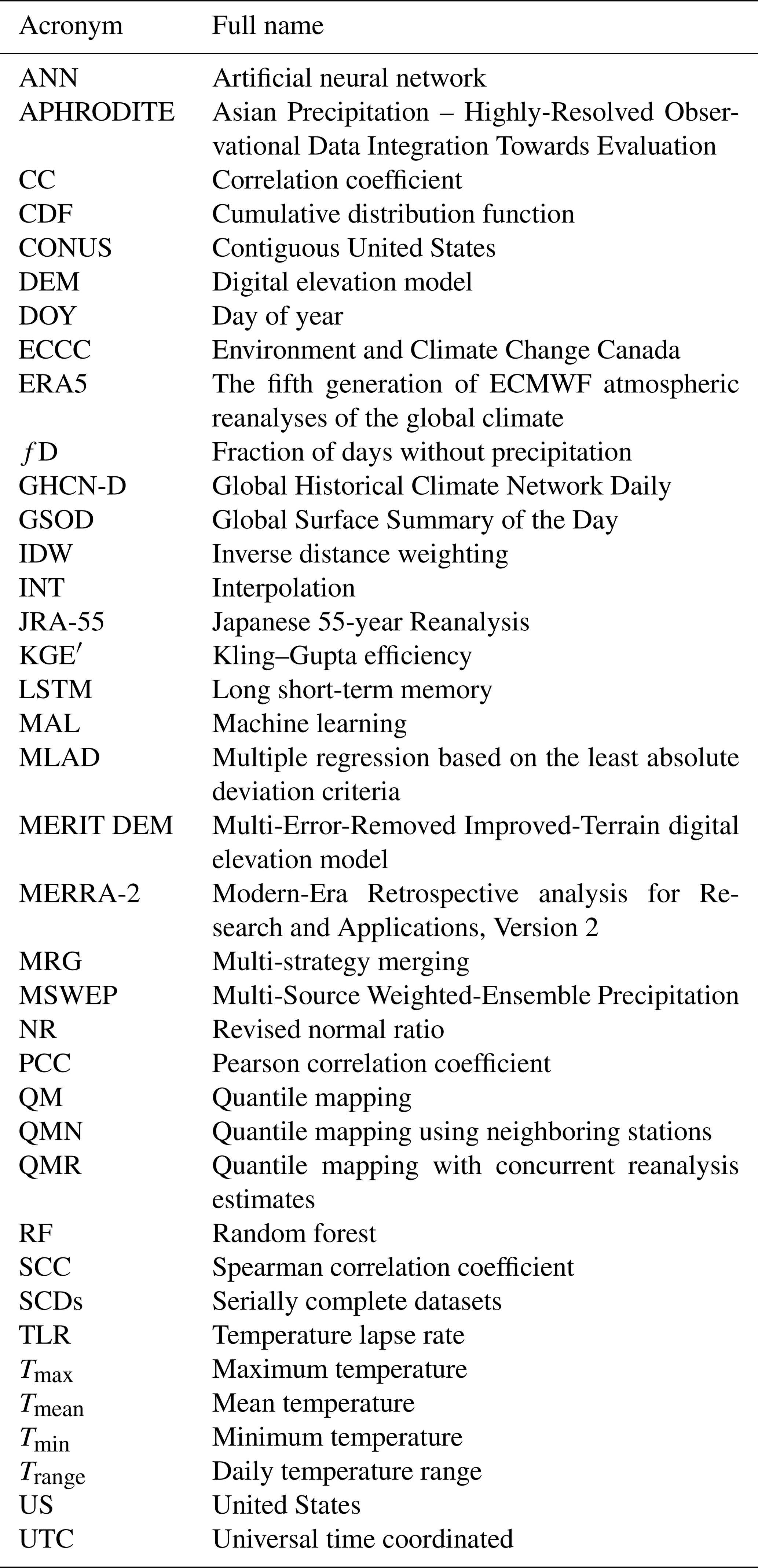
Station-based serially complete datasets (SCDs; see Table A1 for all acronyms) are important for meteorological, climatological, and hydrological studies (Kanda et al., 2018; Ramos-Calzado et al., 2008), such as producing retrospective gridded products (Di Luzio et al., 2008; Kenawy et al., 2013; Newman et al., 2019; Serrano-Notivoli et al., 2019), trend analyses (Knowles et al., 2006; Anderson et al., 2009; Papalexiou and Montanari, 2019), and climatologic index calculations (Alexander et al., 2006; Papalexiou et al., 2018). These SCDs are useful because station-based observational datasets often contain missing values due to factors such as observer absence, instrument failures, and interrupted communication (Hasanpour Kashani and Dinpashoh, 2012). Moreover, station observations failing quality control tests such as outlier and homogeneity checks may not be reliable (Menne et al., 2012), and many stations are only maintained over a relatively short period of time or portions of the year resulting in data gaps that could affect the analysis of climate variability or long-term trends (Rubin, 1976; Stooksbury et al., 1999). Serial completeness is also a critical requirement for real-time station-based applications, which regularly contend with missing data values due to latencies in station reporting, quality control, and processing (Tang et al., 2009).
Many methods have been developed to estimate missing observations and reconstruct time series of meteorological stations that provide point-scale regular observations of atmospheric conditions (Longman et al., 2020). They can be classified as self-contained infilling, spatial interpolation, quantile mapping, and machine learning methods.
-
Self-contained infilling only uses records from the target station to estimate its own missing values. Typical methods include interpolation based on data from the previous and subsequent days or replacing missing values by the long-term mean (Kemp et al., 1983; Pappas et al., 2014). Self-contained infilling, however, only performs well for variables with high temporal autocorrelation such as temperature and is problematic for daily precipitation (Simolo et al., 2010; Teegavarapu and Chandramouli, 2005) and in covering lengthy data gaps.
-
Spatial interpolation uses neighboring stations (identified based on spatial distance or statistical similarity) to estimate data at the target station. Spatial interpolation methods can be divided into two types: the first uses information only from neighboring stations, and common methods include linear interpolation and inverse distance weighting (IDW; Shepard, 1968). The second method needs information from both neighboring and target stations. Typical examples include the revised normal ratio (NR; Young, 1992) and the single best estimator (Eischeid et al., 1995, 2000), both of which use correlation coefficients (CCs) between target and neighboring stations to estimate merging weights. This second type of spatial interpolation also includes more sophisticated methods (e.g., multiple linear regression, optimal interpolation, and kriging) that build a functional relationship between neighboring and target stations (Simolo et al., 2010). Previous studies have shown that multiple linear regression based on the least absolute deviation (MLAD) criteria performs better than many interpolation methods such as IDW, NR, and optimal interpolation in infilling/reconstruction (Eischeid et al., 2000; Kanda et al., 2018).
-
Quantile mapping (QM) is widely used to correct biases in meteorological data (Maraun, 2013; Cannon et al., 2015), and it performs well in estimating missing station data (Simolo et al., 2010; Newman et al., 2015, 2019; Devi et al., 2019). In QM-based estimations, the cumulative distribution functions (CDFs) of observations from neighboring and target stations are derived, and the record at the target station is estimated as the inverse of its CDF using concurrent CDF probability information from neighboring stations. QM can avoid the problem of overestimating wet days in precipitation series and preserve the frequency distribution of time series, which is useful for estimating extreme events (Cannon et al., 2015).
-
Machine learning techniques have been successfully applied to infill station record gaps (Dastorani et al., 2010; Wambua et al., 2016). For example, Coulibaly and Evora (2007) estimated missing daily precipitation and temperature in northeastern Canada using six types of artificial neural networks (ANNs). Ustaoglu et al. (2008) estimated daily temperature using three ANN methods in Geyve and the Sakarya basin, Turkey. Gene expression programming was applied in the estimation of missing monthly rainfall data in Malaysia (Che Ghani et al., 2014). Sattari et al. (2017) recommended that a decision tree algorithm can be used to estimate monthly precipitation due to its simplicity and high accuracy. Serrano-Notivoli et al. (2019) applied the k nearest neighbors regression to reconstruct minimum temperature (Tmin) and maximum temperature (Tmax) observations in Spain to form a gridded dataset.
Previous SCDs have been developed using multiple infilling and reconstruction methods. For instance, Eischeid et al. (2000) produced a daily SCD from 1951 to 1991 for the western United States (US), including 2962 precipitation stations and 2034 temperature stations; Vicente-Serrano et al. (2003) produced a daily SCD from 1901 to 2002 for northeast Spain using 3106 precipitation stations; Di Piazza et al. (2011) built a monthly SCD from 1921 to 2004 for Sicily, Italy, using 247 precipitation stations; and Woldesenbet et al. (2017) produced a daily SCD of precipitation and temperature from 1980 to 2013 for the upper Blue Nile basin using six stations. There is currently no SCD for North America; this means that researchers often must collect station data from different databases, which is time consuming and may cause inconsistencies between studies based on different methods.
Responding to this need, we develop a retrospective 40-year daily SCD for North America (SCDNA) of precipitation, Tmin, and Tmax from 1979 to 2018. Central America and the Caribbean are also covered by SCDNA. The three variables are selected because (1) most stations measure precipitation and temperature, while other variables, such as humidity and wind speed, are measured at fewer stations, and (2) precipitation and temperature data are fundamental inputs for hydrological modeling. Station observations are collected from four global and regional databases and undergo strict quality control to eliminate dubious records. Since the performance of infilling and reconstruction methods differs in space and time, the results from 16 strategies are merged to produce a single deterministic estimate. Finally, the SCDNA is compared to four gridded products to demonstrate its performance and areas for improvement. The SCDNA is expected to have a wide variety of applications in North America, and the methodology can be used to produce SCDs in other regions of the world.
2.1 Meteorological station data
This study uses precipitation, Tmin, and Tmax station data from four databases: the Global Historical Climate Network Daily (GHCN-D; https://www.ncdc.noaa.gov/ghcnd-data-access, last access: 18 October 2019; Menne et al., 2012), the Global Surface Summary of the Day (GSOD; https://catalog.data.gov/dataset/global-surface-summary-of-the-day-gsod, last access: 15 October 2019), Environment and Climate Change Canada (ECCC; https://climate.weather.gc.ca/historical_data/search_historic_data_e.html, last access: 22 December 2019), and the Mexico database from Servicio Meteorológico Nacional under the Comisión Nacional del Agua (Livneh et al., 2015). This study uses daily precipitation totals from each dataset. Only stations with at least 8-year-long precipitation or Tmin and Tmax records between 1979 to 2018 are utilized. The requirement for minimum recording length is different among studies (e.g., Eischeid et al., 2000; Newman et al., 2015). We adopted a relatively short time limitation because (1) 8-year-long records are sufficient for providing basic support for missing value estimation (Fig. S1 in the Supplement) and (2) the open-access dataset and codes enable users to design customized data selection criteria according to their research requirements.
The numbers of stations with at least 8-year-long records are 33 026, 4619, 3634, and 4049 for GHCN-D, GSOD, ECCC, and the Mexico database, respectively (Table 1). Their spatial distributions are shown in Fig. S2 in the Supplement. GHCN-D has compiled a large amount of data from many sources including the Mexico database and ECCC. For identical stations from different sources, we keep the one with the longer observation history, resulting in the exclusion of ∼95 % of stations from the Mexico database and the adoption of ∼91 % of the stations from ECCC. Stations with more than 30 % missing values in the observation period are excluded because they could be seasonal stations or suffer serious instrumentation problems. Stations overlapping in space (same latitude and longitude) and without sufficient metadata for discrimination are merged (see Sect. 3.2). The above screening reduces the available stations from 45 328 to 31 772 (Table 1), yet more stations are discarded due to quality control procedures (Sect. 3.1). The final SCDNA includes 24 615 precipitation, 19 604 Tmin, and 19 611 Tmax stations; note that the numbers of Tmin and Tmax stations differ as quality controls can result in excluding the one and reserving the other in some stations.
Most stations are located in the contiguous United States (CONUS), southern Canada, and Mexico, while few stations are located in high-latitude regions such as the Arctic Archipelago (Fig. 1b and c). The spatial distributions of precipitation and temperature stations are similar except in eastern CONUS where precipitation stations have a higher density.
Table 1Numbers of stations with at least 8-year-long records from 1979 to 2018.
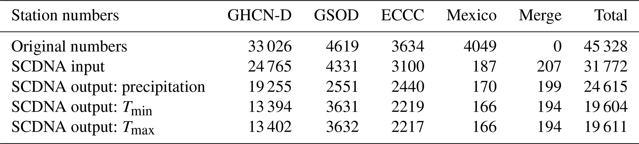
Note that “merge” is derived from stations with overlapping locations from all the other data sources (Sect. 3.1.1).

Figure 1(a) Digital elevation model (DEM; Sect. 2.3) of North America. (b, c) The densities of stations at the resolution for precipitation and temperature, respectively. Tmin and Tmax stations are highly consistent, and thus Tmin is used to represent temperature in (c). The nested black boxes show examples of DEM and station densities.
In North America, more station observations occur in the US than in Canada and Mexico (Fig. 2). The number of samples in the US increases from 1979 to 2018, and there are more precipitation samples than temperature samples. For Canada, the numbers of precipitation and temperature samples are similar and show a decrease from 1988 to 2018; the sample number in 2018 is only 61.76 % of that in 1988. Mexico has more meteorological samples than Canada, yet this number decreases after 1983. The decreasing trend is especially sharp after 2012, which may be due to the delay in data collection or termination of some stations.
Figure 3 shows the fractions of missing values for all stations during the observation period (referred to as ratio-1) and during the entire period from 1979 to 2018 (referred to as ratio-2). For temperature, ∼20 % of the stations have more than 20 % missing values in the observation period (ratio-1), and ∼20 % of the stations have more than 70 % missing values in the entire period (ratio-2). For precipitation, the fraction of missing values is larger. The fractions show strong spatial variations (Fig. S3 in the Supplement). Ratio-2 is smaller for precipitation stations in the western US and temperature stations in central US but is larger in Canada and Alaska. Most stations in Mexico have a higher ratio-1 than other regions in North America, indicating that those stations have notable fractions of missing values during the observation period.
In summary, the curves of ratio-1 indicate that a small number of missing values need infilling during the observation period, while the curves of ratio-2 indicate that extensive reconstruction is needed over the entire period.
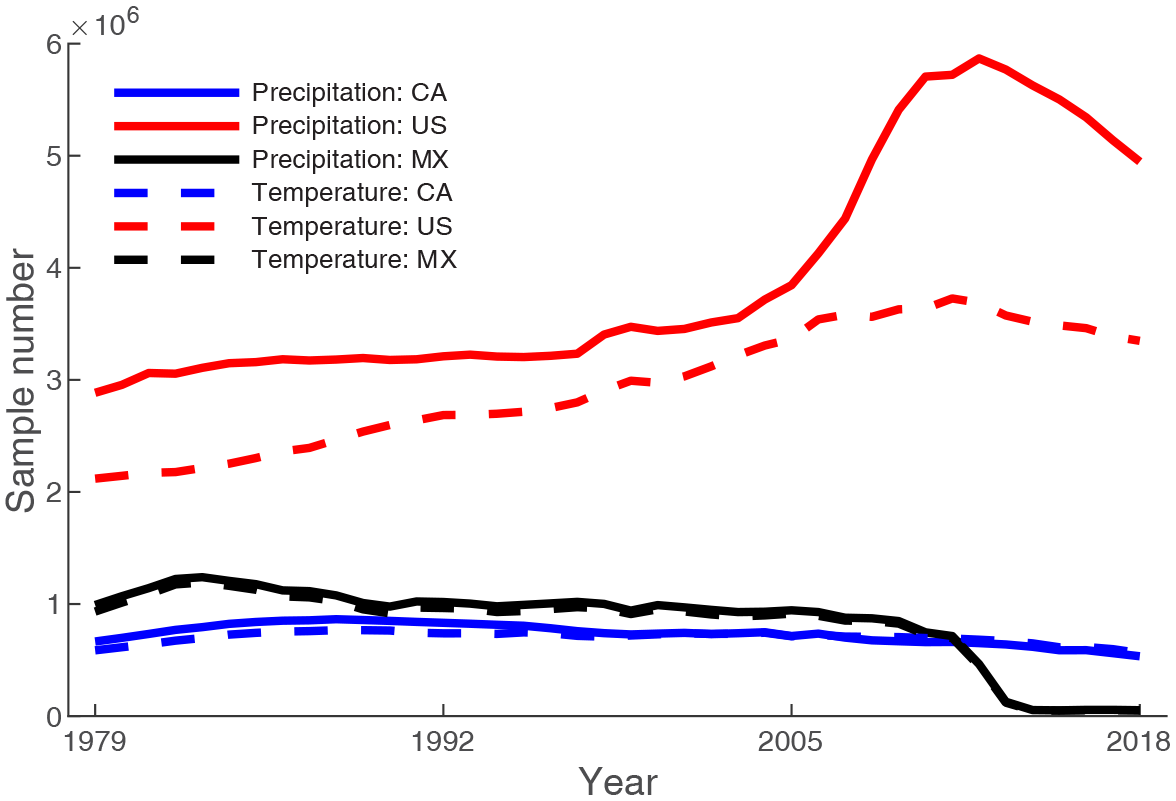
Figure 2Sample numbers of stations for each year from 1979 to 2018. CA represents Canada, US represents United States, and MX represents Mexico. Tmax stations are highly consistent with Tmin stations, and thus Tmin is used to represent temperature. The numbers of samples could be a better indicator than the numbers of stations because many stations have notable missing values.

Figure 3The fraction of missing values for stations with at least 8-year-long records. Ratio-1 is the degree of missingness during the observation period, and ratio-2 is the degree of missingness during the entire period of interest (1979 to 2018). Tmin is used to represent temperature because Tmax shows curves almost overlapping with Tmin.
Many types of precipitation and temperature measurement instruments are used at stations from different sources. For example, the Type B rain gauge has been used by Environment Canada since the 1970s for most weather stations (Devine and Mekis, 2008; Wang et al., 2017), while tipping bucket and weighing rain gauges are also used in some stations (Metcalfe et al., 1997). Nipher-shielded snow gauges have been used by some synoptic stations, while ruler measurements are still used by more stations (Mekis and Brown, 2010). Station data in the US are from many organizations or programs with different instrument configurations. For instance, the standard rain gauge is used by the Cooperative Observer Program, while snow telemetry uses storage-type gauges or tipping buckets. A better understanding of instrument specifications and historical changes is important for climate studies (Pielke et al., 2007; Whitfield, 2014; Ma et al., 2019). A detailed summary of station instruments is provided in the documentation of the dataset (https://doi.org/10.5281/zenodo.3735533).
2.2 Reanalysis products
We use reanalysis precipitation, Tmin, and Tmax from the fifth generation of European Centre for Medium-Range Weather Forecasts (ECMWF) atmospheric reanalyses of the global climate (ERA5; Copernicus Climate Change Service (C3S), 2017), the Japanese 55-year Reanalysis (JRA-55; Kobayashi et al., 2015), and the Modern-Era Retrospective analysis for Research and Applications, Version 2 (MERRA-2; Gelaro et al., 2017) (see Table 2). The three products are chosen because they are representative products from different international organizations, and they or their predecessors (ERA-Interim, JRA-25, and MERRA) have been widely used by researchers. ERA5 and JRA-55 do not provide daily outputs; thus, daily precipitation is accumulated from sub-daily estimates, while daily Tmin and Tmax are estimated by the sub-daily minimum and maximum temperature values. Gridded reanalysis precipitation is linearly interpolated to match point-scale station data, and Tmin and Tmax are downscaled using temperature lapse rate (TLR; see Sect. 3.1).
Table 2Information on the three reanalysis products.
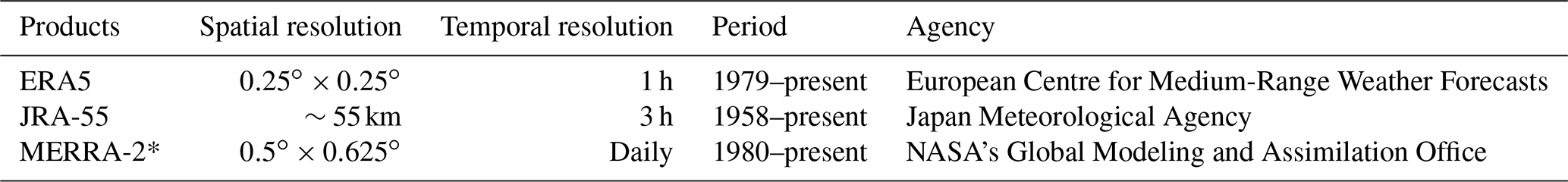
* MERRA-2 provides outputs in temporal resolutions from 1 h to 1 month; here we use daily values.
2.3 Auxiliary data
The Multi-Error-Removed Improved-Terrain digital elevation model (MERIT DEM) at a 3 s (∼90 m at the Equator) resolution (Yamazaki et al., 2017) is used in this study. To enable temperature downscaling, the high-resolution DEM is spatially averaged to the original resolutions of ERA5, MERRA-2, and JRA-55 (Table 2). The MERIT DEM data may be slightly different than the DEM data used in the three reanalysis products, and this will have a limited impact on missing data estimation (Sect. 3.3.2).
The Multi-Source Weighted-Ensemble Precipitation (MSWEP) V2.2 dataset (Beck et al., 2017, 2019) is utilized for the comparison with the SCDNA developed by this study. MSWEP merges data from ground observations, satellite products, and reanalysis models and performs better than all products used for merging (Beck et al., 2019). The comparison can show whether the SCDNA is a better choice than MSWEP to fill in gaps in station precipitation observations.
The methodology to produce the SCDNA includes three primary steps (Fig. 4): (1) preparing a unified precipitation and temperature database from multiple sources (Sects. 2.1 and 3.1); (2) downscaling reanalysis estimates (Sects. 2.2 and 3.2) that are used in QM-based and machine-learning-based data estimation (Sect. 3.3) and in comparison with the SCDNA (Sect. 4.5); and (3) producing the SCDNA from 1979 to 2018 based on 16 strategies (Sect. 3.3). The following subsections summarize the work in each step of the methodology (Sect. 3.1, 3.2, and 3.3), as well as the approach used to evaluate the performance of the method (Sect. 3.4).

Figure 4Flowchart of the production of the SCDNA, including station data preparation, reanalysis product processing, and missing data infilling and reconstruction.
In this study, infilling refers to the estimation of missing values during the observation period, while reconstruction refers to estimating values outside of the observation period when no station record is available (Fig. 5). Station records that fail quality control are treated as missing values.
3.1 Prepare a unified precipitation and temperature database
3.1.1 Merging of stations based on location
Stations are merged if their latitude and longitude match other stations. The problems of overlapping locations are caused by the identification alteration of one station for different periods, recording/rounding bias of station location information, inconsistent naming rules of different sources, and other factors. Although it is possible that multiple stations are deployed in the same location for experimental aims, location merging is done to preserve internal consistencies as inconsistent records at the same location are self-contradictory.
The method for location merging includes several steps. First, overlapping stations are extracted and grouped. Stations within the same group that have nonoverlapping recording periods are simply merged into one time series. Otherwise, the Spearman's rank CC (SCC) between precipitation series from all station pairs in the group is calculated. For SCC<0.7, the station group is discarded due to large discrepancies; for , the discrepancy is considered tolerable, and the station with the longest record is kept; for SCC>0.9, stations are considered highly correlated, and their data are merged into one time series, while for overlapping periods, the station with the longest record is used.
Overall, 1240 stations are involved in location merging, stratified in 586 station groups. Around 10 % of the groups contain more than two stations, and the largest group contains five stations. After location merging, only 207 groups are kept and merged into unified times series (Table 1). Despite the steps taken above, the merged series could contain inhomogeneities due to the combination of records from multiple stations.
3.1.2 Quality control
To ensure station observations undergo strict and comprehensive quality control, we adopted the methods used to produce previous station-based datasets. For Tmin and Tmax, we followed the method designed by Durre et al. (2010) which is adopted by GHCN-D (Menne et al., 2012). The procedures include five types of checks: integrity checks, outlier checks, internal and temporal consistency checks, spatial consistency checks, and extreme mega consistency checks. A few of the procedures in Durre et al. (2010) require other variables such as snowfall and thus are not adopted in this study. In addition, the quality flags in this study are partly different from those of GHCN-D because of the different sources, numbers, and temporal periods of stations.
For precipitation, quality control procedures consist of three parts. The first part is similar to that for temperature. The second part (four types of checks) follows procedures designed by Hamada et al. (2011) which have been adopted by the Asian Precipitation – Highly-Resolved Observational Data Integration Towards Evaluation (APHRODITE; Yatagai et al., 2012). The third part (two types of checks) adopts strategies by Beck et al. (2019) used in the production of MSWEP. Note that although Durre et al. (2010) and Hamada et al. (2011) share some common traits for precipitation, both of them are adopted to ensure quality control reliability. The details of quality checks are in Appendix B.
3.2 Downscale reanalysis data
The reanalysis temperature estimates are downscaled to match point-scale station observations using temperature lapse rate (TLR) according to the following:
where TR is 2 m reanalysis air temperature, Ts is downscaled temperature, Δh is the height difference between station elevation and reanalysis grid elevation. TLR shows notable spatiotemporal variations (Minder et al., 2010), and estimating TLR based on ground observations over a large domain is difficult due to the sparsity of stations. Yet recent studies show that reanalysis outputs offer an alternative to estimating gridded TLR (e.g., Gao et al., 2012). The gradient of air temperature at different pressure levels above the ground can be used to approximate near-surface TLR (Gao et al., 2012, 2018; Gruber, 2012). Tang et al. (2018b) compared eight temperature downscaling methods in CONUS and found that methods based on reanalysis-derived TLR can achieve higher accuracy compared to fixed TLR (e.g., −6.5 ) or statistical interpolation downscaling methods. Hence, this study uses the linear regression slope between MERRA-2 air temperature and geopotential heights from 300 to 1000 hPa pressure levels to represent TLR for each month at a resolution of (Table 2). MERRA-2 is used because it directly provides monthly data and masks temperature data if the pressure level is below the land surface. The choice of pressure levels needs further investigation because relationships between vertical and near-surface temperature vary with regions. Complicated TLR phenomena such as inverse lapse rate are not considered for simplicity. The climatological mean of TLR (Fig. S4 in the Supplement) decreases from in the northeast continent (i.e., Canadian Arctic Archipelago) to in the southwest continent (i.e., Rocky Mountains in CONUS). The smaller TLR magnitude at high latitudes is consistent with previous studies (e.g., Gardner et al., 2009; Marshall et al., 2007).
3.3 Produce the serially complete dataset
To produce the high-quality SCDNA for North America, we use 16 strategies: four based on quantile mapping with neighboring stations (QMN; e.g., Longman et al., 2019; Newman et al., 2015, 2019), four on quantile mapping with concurrent reanalysis estimates (QMR), four using spatial interpolation methods (INT; e.g., Eischeid et al., 2000; Kanda et al., 2018; Woldesenbet et al., 2017), two using machine learning methods (MAL; e.g., Dastorani et al., 2010; Wambua et al., 2016), and two multi-strategy merging (MRG) methods. Merging multiple infilling/reconstruction methods can provide a better estimation than individual methods, as shown by previous data merging and gap infilling studies (e.g., Eischeid et al., 2000; Beck et al., 2017, 2019; Ma et al., 2018).
We generate estimates for every station and every day from 1979 to 2018 (Fig. 5). The estimates from these 16 strategies and the SCDNA are evaluated using station observations, and the performance of the SCDNA is compared to four benchmark gridded products. Then, the estimates of the SCDNA are corrected for further accuracy improvement. Finally, estimates are replaced by station observations when observations exist and pass quality control checks. The variance and spatial correlation analyses are performed to compare the statistical properties of station observations and estimates (see Sect. 4).
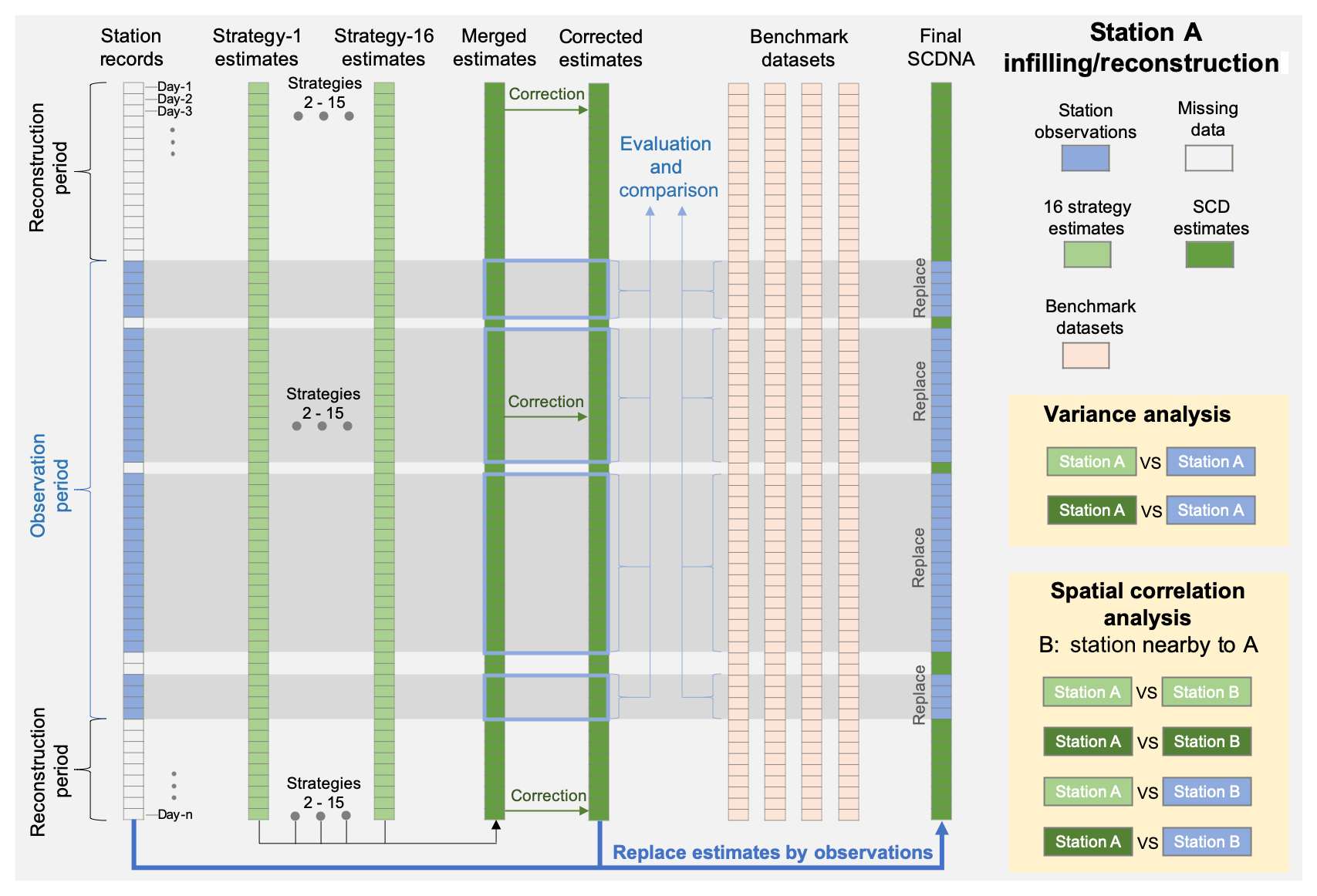
Figure 5Diagram of the infilling and reconstruction for a specific station (referred to as A). The entire period from 1979 to 2018 is divided into the observation period and the reconstruction period. The data flows of variance and spatial correlation analyses are shown in the nested yellow boxes. Station B is a nearby station to A.
Only stations with at least 3000 valid values are included in the infilling and reconstruction effort. The nine steps (termed Step-1 to Step-9) of SCDNA production are described below. Unless otherwise stated, the steps are implemented for each target station (s), each variable (precipitation, Tmin, and Tmax), and each day of the year (DOY, i.e., 1–366).
3.3.1 Data extraction
-
Step-1. Spatiotemporally concurrent reanalysis estimates (ERA5, JRA-55, and MERRA-2) are extracted, including precipitation, Tmin, Tmax, and TLR. Precipitation is linearly interpolated from gridded reanalysis estimates, and temperature is downscaled (i.e., corrected for the elevation difference between the reanalysis grid cell and the station elevation) based on TLR (Sect. 3.1).
-
Step-2. Neighboring stations (at least 1 and at most 30) with at least an 8-year overlapping period with station s are found within the search radius of 200 km. These stations are ranked from closest to farthest according to their CC with the target station. The SCC is used for precipitation, and Pearson CC (PCC) is used for Tmin and Tmax. CC is calculated using data within a 31 d window centered around the current DOY from all years.
-
Step-3. The empirical CDFs of s, neighboring stations, and reanalysis estimates are obtained using data within the same 31 d window.
3.3.2 Infilling and reconstruction
-
Step-4. For each day (d) corresponding to the DOY, the estimated data are acquired based on 16 strategies which are divided into five groups.
Group 1: quantile mapping with neighboring stations (QMN)
-
QMN-1. For all neighboring stations with valid records, the station with the highest CC in Step-2 is selected. The estimated data for s and d are obtained using Eq. (2):
where Xi is precipitation or temperature for d from the selected neighboring station i, Fi is the empirical CDF of i corresponding to the DOY, is the inverse CDF of s corresponding to the DOY, and Xs is the estimated data.
-
QMN-2. For all neighboring stations with observations, estimated values are obtained using Eq. (2) which are merged based on Eq. (3):
where n is the number of neighboring stations, is the QM-based estimate from i, and Wi is the weight calculated using Eq. (4). CCi is the CC (SCC or PCC) between data from s and i corresponding to the DOY. Wi is assigned 0 if CCi is negative.
-
QMN-3. Similar to QMN-2 but the weight is calculated according to the distance (Di) between s and i based on Eq. (5). Although the exponent of distance (k) varies in different studies, −2 is the most common choice (Teegavarapu and Chandramouli, 2005):
-
QMN-4. The median of QMN-1 to QMN-3 is used as the estimated data. The strategy of using median values is the same with Eischeid et al. (2000), which could be closer to actual observations than QMN-1 to QMN-3.
Group 2: quantile mapping with reanalysis products (QMR)
Reanalysis products provide useful information for SCDNA production as (1) remote regions may not have enough neighboring stations and (2) neighboring stations also have missing values which could result in gaps of estimates at the target station.
-
QMR-1–QMR-3. They are similar to QMN-1, but the neighboring station is replaced by concurrent ERA5, JRA-55, and MERRA-2 estimates, respectively.
-
QMR-4. The median of QMR-1 to QMN-3 is used as the estimated data.
Group 3: interpolation (INT)
The three interpolation methods used in this study are MLAD (referred to as INT-1), NR (referred to as INT-2), and inverse distance weighting (IDW; referred to as INT-3). They are described below. Following Eischeid et al. (2000), neighboring stations with a CC lower than 0.35 are excluded. The remaining stations are ranked from high CC to low CC. A maximum of four neighboring stations are used in the interpolation. For Tmin and Tmax, direct interpolation from neighboring stations to s could be biased due to the elevation differences between stations. Temperature data from neighboring stations are downscaled to the elevation of s based on Eq. (1).
-
INT-1. MLAD minimizes the sum of absolute errors. It is more robust than regression based on least squares because, while least square estimation is effective when the errors are normally distributed and independent, environmental variables, especially precipitation, often violate the assumption of normality (Eischeid et al., 2000). MLAD has been well documented with better performance in gap infilling than other interpolation methods (Eischeid et al., 1995, 2000; Kanda et al., 2018; Young, 1992). The formula is shown in Eq. (6):
where ci (i=0, 1, …, n) is regression coefficients estimated using data within a 31 d window for each DOY. Different d values corresponding to the same DOY could have different combinations of neighboring stations due to the limitation of observation availability. MLAD is performed for each combination to ensure that effective estimates are available for all days.
-
INT-2. NR is an interpolation method proposed by Paulhus and Kohler (1952) and modified by Young (1992). The modified version is adopted in this study, which combines information from neighboring stations by replacing with Xi in Eq. (3). The weight is calculated using Eq. (7):
where Ni is the number of samples used to calculate CCi between s and i. The SCC is used for precipitation, and the PCC is used for temperature.
-
INT-3. IDW is one of the most common interpolation methods. It is implemented similar to NR in that the inverse squared distance, as shown in Eq. (5), is used as the weight.
-
INT-4. The median of INT-1, INT-2, and INT-3 is used as the estimated data.
Group 4: machine learning (MAL)
The two MAL methods used in this study are ANN (referred to as MAL-1) and random forest (RF; referred to as MAL-2; Breiman, 2001). Unlike QMN, QMR, and INT that are carried out for each DOY, MAL uses complete observation records of s to ensure that ANN and RF are trained with enough values. MAL models are trained using the first 70 % of observations and tested using the remaining 30 % of observations. The MAL models' validation based on the 30 % of observations can indicate their performance in the reconstruction period.
The input data are from neighboring stations and concurrent reanalysis estimates. For each s, neighboring stations are determined in a way similar to Step-2, but the CC is calculated using data from the entire observation period. Neighboring stations with a CC lower than all reanalysis products (ERA5, JRA-55, and MERRA-2) are excluded. The remaining neighboring stations and three reanalysis products form a complete repository of input features. Then, for each day that s has no observation, the input features are extracted from the repository in three steps: (1) neighboring stations without observations for the day are excluded, (2) the remaining neighboring stations and reanalysis products are ranked according to their CC with s, and (3) at most five stations/reanalysis products with the highest CC are selected. In this way, s will have multiple combinations of input features to ensure that all days with missing values have estimates. All combinations are used to train and test the ANN and RF models, resulting in multiple estimated series for s. The final estimates of s are generated in three steps: (1) the Kling–Gupta efficiency (KGE′; Kling et al., 2012) of all estimated series is calculated using all observations of s and ranked from high to low KGE′ (see Sect. 3.4 for definition of KGE′), (2) the series with a higher KGE′ is used to constitute the estimates of s in sequence, and (3) the second step is repeated until there are no missing values for s. This approach ensures that the “best” and complete estimates are provided for s.
-
MAL-1. A four-layer ANN is used. The input layer has a maximum of five nodes (depending on the number of input features), the two hidden layers both have 20 nodes, and the output layer has one node for generating precipitation or temperature estimates. The transfer functions are hyperbolic tangent sigmoid for hidden layers and linear for the output layer. The training function is resilient backpropagation. The model is trained using the first 50 % of data, validated using the subsequent 20 % of data, and tested using the final 30 % of data.
-
MAL-2. An RF model with 50 trees is built with 70 % training data and 30 % testing data. The minimum number of samples per tree leaf is five. The input nodes depend on the number of input features like MAL-1.
Group 5: multi-strategy merging (MRG)
-
MRG-1. KGE′ is used to rank the performance of the 11 strategies (QMN-1 to QMN-3, QMR-1 to QMN-3, INT-1 to INT-3, and MAL-1 to MAL-2) as a CC cannot reflect the magnitude difference (e.g., bias) between target and reference series. The first three cases of the 11 strategies are merged using squared KGE′ as the weight. The individual weight is assigned 0 if KGE′ is negative.
-
MRG-2. The median of the three selected strategies in MRG-1 is used as the estimated data.
3.3.3 Generating serially complete records
-
Step-5. In this step, Step-3 and Step-4 are repeated based on 70 % of data of s from the observation period. Then, the KGE′ of estimates from all strategies is calculated using the remaining 30 % of observations. MAL-1 and MAL-2 are not repeated because they are trained on 70 % of observations. Although the evaluation samples are different among stations, the results are reliable and stable as shown in the results section. This step is implemented because QMN-1 to QMN-4, QMR-1 to QMR-4, and INT-1 in Step-4 use all data of s from the observation period to select stations, estimate empirical CDFs, and carry out regression. This potential overfitting problem could lead to the better performance of these strategies in the observation period but worse performance in the reconstruction period. KGE′ calculated in Step-4 can represent the accuracy of estimates in the observation period, while KGE′ calculated in Step-5 can represent the accuracy of estimates in the reconstruction period.
-
Step-6. In the observation period, the strategy with the highest KGE′ in Step-4 is selected to contribute the extension/reconstruction to the SCDNA. In the reconstruction period, first, the strategy with the highest KGE′ in Step-5 is determined; then, the estimates from the corresponding strategy in Step-4 are used to constitute the SCDNA because the empirical CDF and regression based on all observations in Step-4 could be more representative than the 70 % of observations in Step-5.
-
Step-7. Estimates in Step-6 are corrected for certain climatological biases using station data from the observation period. Precipitation estimates are often subjected to wet-day bias. Two methods are implemented to address this problem. First, QM is performed based on the CDF of s in Step-3. However, QM may reduce the accuracy of estimated precipitation in some cases, for which the method used in Beck et al. (2019) is adopted. This method subtracts a tiny value (0.01 mm) from the original precipitation series and rescales the series to restore the original mean value. This operation is repeated until the estimated series shows an equal number of wet days () with observations of s. In addition to wet-day bias correction, mean value correction is implemented. The ratio between the mean values of precipitation estimates and observations is calculated for the observation period, which is used to rescale estimated series in both observation and reconstruction periods. For Tmin and Tmax, QM correction and mean value correction are also implemented.
-
Step-8. The accuracy of the SCDNA is evaluated and compared to benchmark datasets based on actual observations (Fig. 5). Then, the estimates are replaced by observations whenever possible to generate the final SCDNA. Very occasionally, estimated Tmin could be larger than estimated Tmax, for which Tmax is replaced by the maximum Tmax and Tmin is replaced by the minimumTmin of the estimates from the 16 strategies.
-
Step-9. The serially complete data of SCDNA is quality controlled again using methods introduced in Sect. 3.1.2 to exclude stations with unreliable estimates.
3.4 Evaluate the precipitation and temperature estimates
KGE′, which was proposed by Gupta et al. (2009) and modified by Kling et al. (2012), is used to support the merging of different strategies (Sect. 3.3) and the evaluation of the estimated precipitation and temperature:
where r is the PCC, β is the bias ratio, γ is the variability ratio, μ is the mean value, and σ is the standard deviation (SD). The subscripts e and o represent estimated and reference time series, respectively. KGE′ ranges from negative infinity to 1. If two series exactly match, the KGE′ is 1. A β or γ value smaller/larger than 1 indicates that the mean value or variability of observations is underestimated/overestimated.
In Sect. 4, the evaluation during the observation period is based on the complete station observations (i.e., Step-4 in Sect. 3.3.2), while the evaluation during the reconstruction period is realized using 30 % of independent station observations (i.e., Step-5 in Sect. 3.3.3). Unless otherwise stated, SCDNA estimates in Sect. 4 are after correction (Step-7 in Sect. 3.3.3). In Sect. 4.5, SCDNA estimates are compared with gridded products (ERA5, JRA-55, MERRA-2, and MSWEP). In addition to the three SCDNA variables (precipitation, Tmin, and Tmax), mean temperature (Tmean, the mean of Tmin and Tmax) and daily temperature range (Trange, the difference between Tmax and Tmin) are also included. The involvement of Trange can contribute to a more objective comparison between SCDNA and reanalysis products because the TLR-based downscaling of reanalysis temperature contains uncertainties which could affect the evaluation of Tmin, Tmax, and Tmean. Although there exist differences between the TLRs of Tmin and Tmax, Trange can reduce the effect of scale mismatch between gridded reanalysis temperature and point station temperature on evaluation results.
4.1 Comparison of infilling and reconstruction strategies
The value of a given infilling/reconstruction strategy can be quantified by the extent that a strategy is selected for use in the final SCDNA dataset. In this sense, the contribution ratios define the proportion of estimates that come from a specific strategy. Figure 6 shows that the contribution ratios of QMN, QMR, and INT to missing value estimation are generally smaller than 20 % in North America. Please note that QMN refers to all strategies within this group unless the strategy number is specified right after QMN. This also applies to other groups. QMR shows the smallest contribution ratios for almost all stations among the five groups. Compared to other regions in North America, contribution ratios of QMR are higher for precipitation stations in the western US and temperature stations in Mexico. INT shows lower contribution ratios in the Rocky Mountains compared to the western US, indicating that statistical interpolation without considering topographic effect is subjected to substantial uncertainties in complex terrain. MAL shows notably higher contribution ratios than QMN, QMR, and INT, particularly for Tmin and Tmax. The ratios of MAL are higher than 20 % for ∼30 % of precipitation stations, ∼65 % of Tmin stations, and ∼68 % of Tmax stations. MRG has the highest contribution ratios throughout North America. The average contribution ratios of MRG are 59.88 %, 41.59 %, and 40.56 % for precipitation, Tmin, and Tmax, respectively. For precipitation, MRG is particularly effective in high-latitude regions (northern Canada and Alaska), the western US, and Mexico.
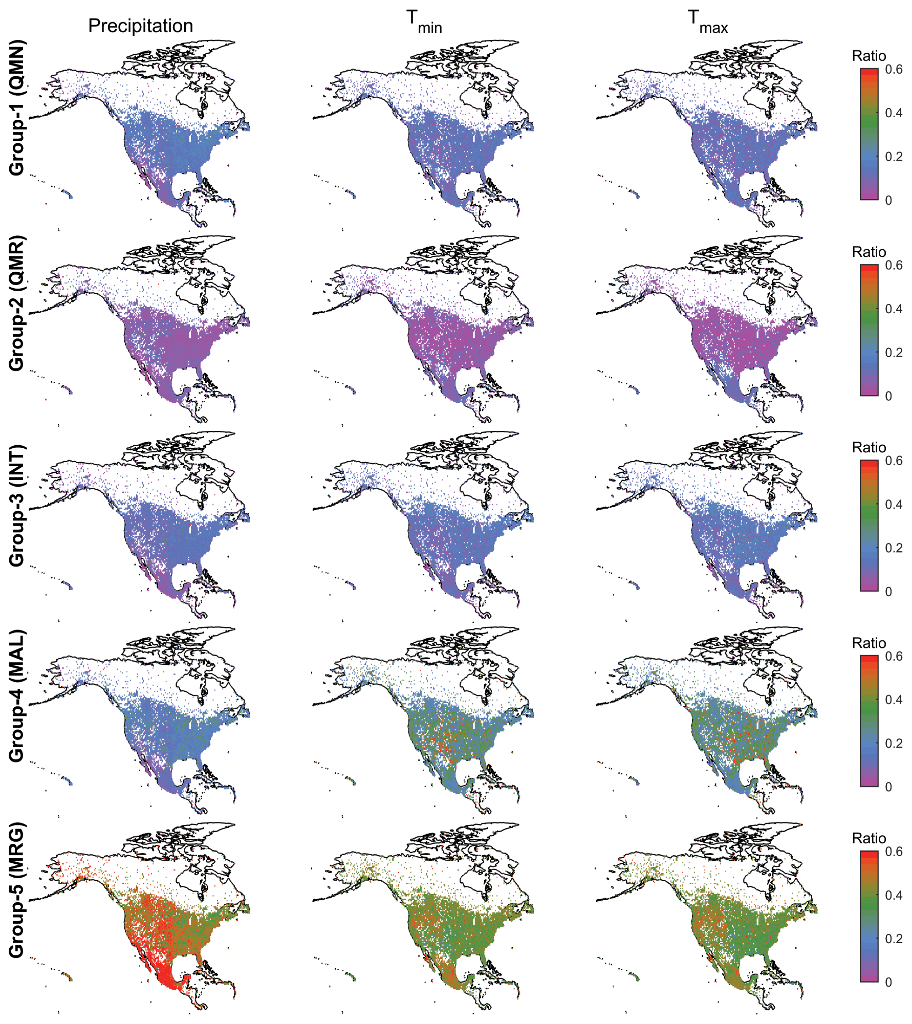
Figure 6The contribution ratios of estimates from five infilling/reconstruction groups to the missing values of all stations from 1979 to 2018. The three columns from left to right represent precipitation, Tmin, and Tmax, respectively. The five rows from top to bottom represent Group-1 (QMN), Group-2 (QMR), Group-3 (INT), Group-4 (MAL), and Group-5 (MRG), respectively. The maps are at a resolution of 0.5∘. The ratio for each grid cell is the mean value of all stations within this grid cell.
Figure 7 shows the KGE′ and contribution ratios of 16 strategies. The KGE′ of estimated precipitation is lower than that of estimated Tmin and Tmax due to the stronger spatial and temporal homogeneity of temperature (Fig. 7). The median KGE′ values of Tmin and Tmax are generally above 0.9, and the accuracy of estimated Tmax is higher than that of Tmin. The KGE′ during the reconstruction period is smaller than that during the observation period, which is particularly obvious for QMN, QMR, and INT-1 compared to other strategies, because QMN and QMR transfer CDF during the observation period to other periods, and INT-1 transfers the regression relationship during the observation period to other periods. MAL suffers a slight degradation in the reconstruction period, and the better performance of MAL-2 than MAL-1 shows that RF could be a better choice than ANN to estimate missing data. For MRG, the differences of KGE′ between the two periods are relatively small. For example, the median KGE′ values of MRG-1 for Tmax are 0.99 and 0.98 for the observation and reconstruction periods, respectively. MRG also shows higher KGE′ and a narrower quantile range than other strategies, particularly for precipitation, as it benefits from merging estimates from multiple strategies.
Regarding contribution ratios (Fig. 7), strategies with higher KGE′ often have larger contributions to the estimated series. However, this is not always true because the selection of strategies is performed for each DOY. Note that the contribution ratios of MAL-2 are even higher than MRG-1 during the observation period for Tmin and Tmax, although MRG-1 achieves higher KGE′ than MAL-2 for most stations. This is because MAL-2 could be the best choice for more DOY than MRG-1 even though MRG-1 may achieve the best overall performance. An example using Tmin data from one station is shown in Fig. S5 in the Supplement.
In the reconstruction period when observations are absent, the contribution ratios of MAL-2 decrease drastically compared to the observation period, contributing to the increased ratios of other strategies (particularly MRG-1). Although QMR shows the lowest contribution ratios, reanalysis products have implicit contributions to other strategies (e.g., MAL and MRG). Overall, MRG-1 shows much higher contribution ratios than all the other strategies (including MRG-2) during the reconstruction periods, indicating that it is the most important strategy in missing value estimation. Hence, combining information from multiple strategies is more reliable, and KGE′-based merging is more effective than the median-value-based estimation.
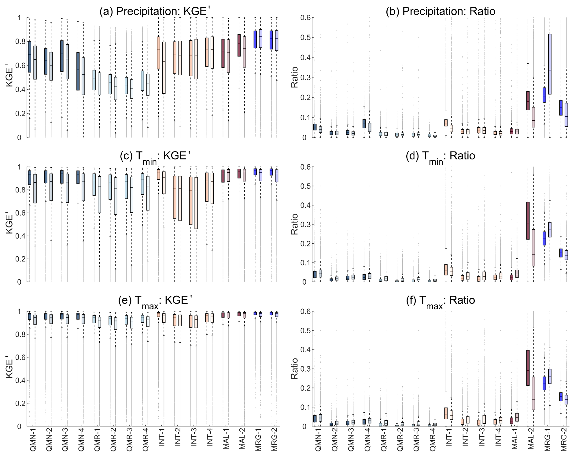
Figure 7Boxplots of (a, c, e) KGE′ and (b, d, f) the contribution ratio of 16 strategies for all stations. Each strategy corresponds to two boxes in each panel; the left one with the darker color represents the observation period, and the right one with the lighter color represents the reconstruction period. The line within the box is the median. The upper and lower edges of the box represent the 25th and 75th percentiles, respectively. Values more than 1.5 times the interquartile range away from the upper or lower edges are outliers (dots).
4.2 Impact of reconstruction on spatial correlation and series variance
All infilling/reconstruction strategies except QMR rely on information from neighboring stations; this could affect the spatial correlation structure and the variance of SCDNA series. Space–time correlations and other properties (e.g., intermittency of precipitation) are important considerations because they can influence the performance of follow-on applications that use the SCDNA as input. Theoretically, QMN strategies could significantly inflate the spatial correlation but retain variance of station observations. The spatial correlation inflation in INT strategies could be lower, but the variance would be underestimated due to smoothing. QMR-1 is used as an example to demonstrate the effect of QM on the spatial correlation and series variance (Fig. S6 in the Supplement) because QMN uses different station combinations for every DOY, which would mask the effect of QM on final estimates. If the ERA5 used by QMR-1 is replaced by station observations, the results should be generally consistent. According to Fig. S6, the spatial correlation is substantially inflated by QMR-1, particularly for Tmin and Tmax, while the SD of QMR-1 estimates is very close to that of observations. This supports the design of estimating missing data using neighboring stations for each DOY as otherwise the inflation of CCs could be very substantial for the entire period.
The spatial correlation based on station observations (Fig. 8a, d, and g) shows obvious seasonal variations with CCs lower in the warm season and higher in the cold season. The seasonality of CCs for Tmax is weaker compared to that for precipitation and Tmin. The SCDNA estimates capture the seasonal patterns but underestimates the variation (Fig. 8b, e, and h) because the inflation of spatial CCs is larger in the warm season than cold season (Fig. 8c, f, and i). Moreover, the inflation is larger for neighboring stations with a lower correlation with the target station. We tested selected neighboring stations according to their distance from the target station, and similar results were acquired. For precipitation, the median CC differences of all stations are close to 0.1 in the cold season and range between 0.1 and 0.15 in the warm season. For Tmin, the median CC differences are generally between 0.05 and 0.15. The CC differences of Tmax are relatively homogeneous for different seasons and generally fluctuate between 0.05 and 0.1. The inflation of CC is because (1) the estimates from the 10 neighboring stations and the target station are generally derived using highly overlapped information (Sect. 3.3.1) and (2) the estimation is realized for each DOY for all strategies except MAL, meaning that calculating CCs for each DOY shows the inflation to the largest extent.
The final SCDNA replaces estimates by observations, which can largely relieve the inflation of spatial correlation (Fig. S7 in the Supplement) depending on the degree to which observations are present in the record. For Tmin and Tmax, the CC is very close to that based on observations; for precipitation, the correlation in wintertime is even lower than that based on observations.
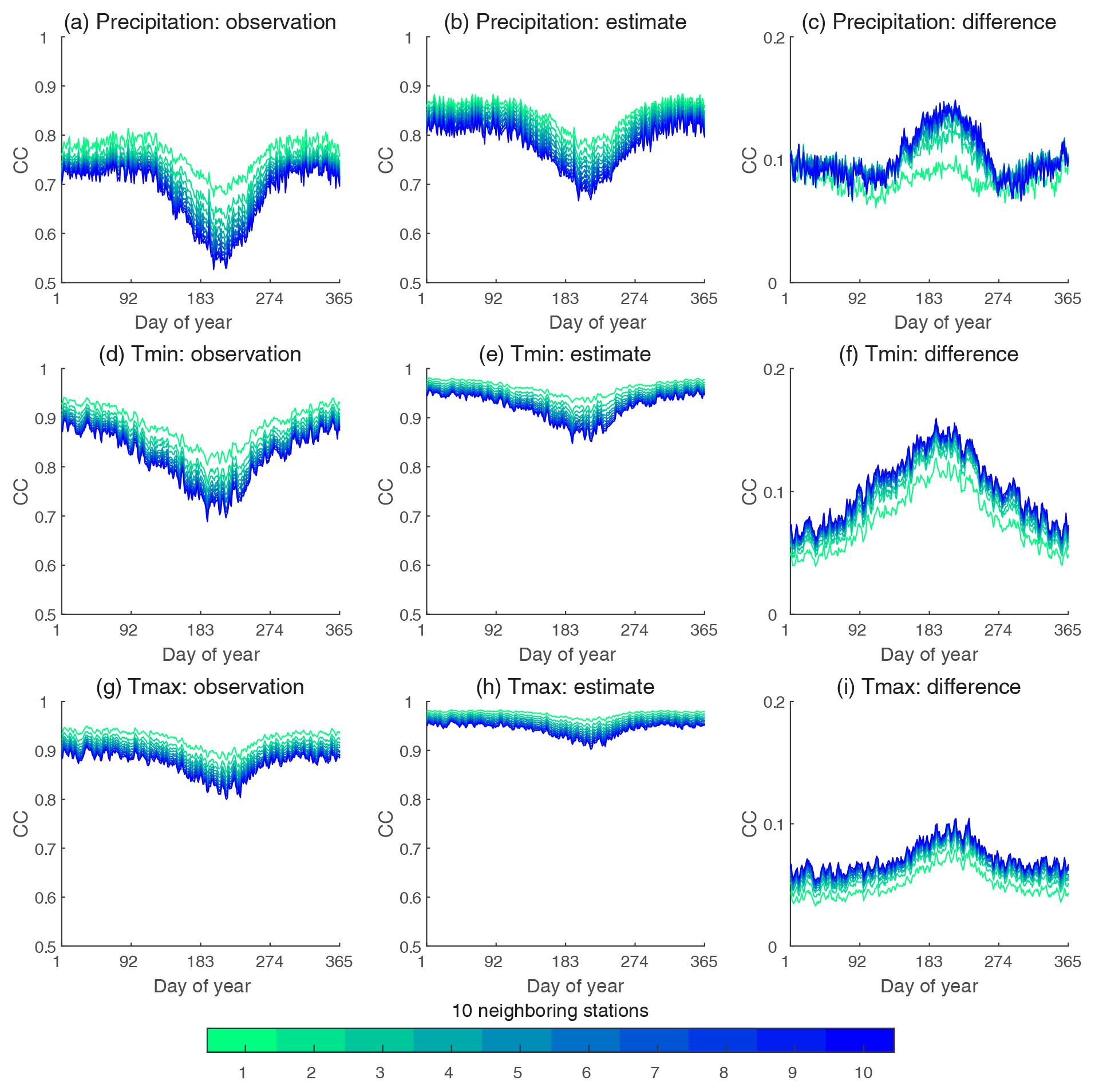
Figure 8CC between target and neighboring stations for all DOY using station observations (the first column), SCDNA estimates (second column), and differences between SCDNA- and observation-based CCs (the third column). The CC is calculated for the observation period. For each target station, 10 neighboring stations are selected according to the correlation between time series from target and neighboring stations. Smaller numbers represent a higher correlation. For example, station 1 represents the neighbor with the highest CC in comparison to the target station. Each curve represents the median CC of all stations.
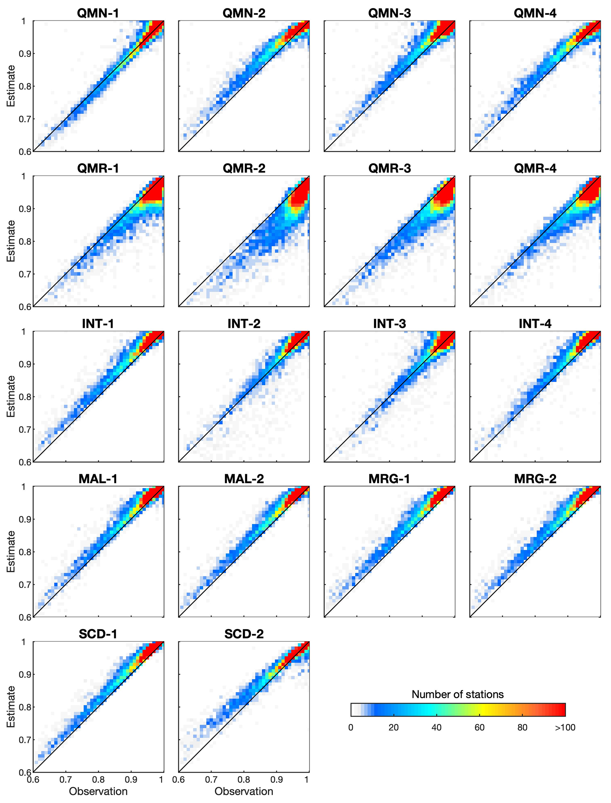
Figures 9 and 10 show CCs between estimates at the target station and observations at the neighboring station. For precipitation, most strategies exhibit a similar spatial correlation structure with observations for most stations. QMR largely underestimates CCs compared to observations, which should be attributed to the differences between precipitation of reanalysis products and stations. There are notable differences in different strategies within one group. For example, QMN-1 shows larger inflation when observation-based CCs are higher, which is not seen in QMN-2 to QMN-4. This is probably because QMN-1 only uses information from the one neighboring station with the highest correlation with the target station for each DOY. The higher observation-based CC in Fig. 9 means this neighboring station could be more frequently used by QMN-1 to estimate data for the target station, resulting in the larger inflation of the CC. Another example is that INT-1 underestimates the CC for 68.75 % of stations, whereas INT-2 to INT-4 overestimates the CC for almost all stations. For SCD-1, the inflation of the CC is observed for 76.60 % of stations, whereas the magnitude of overestimation is smaller than that in Fig. 8. The mean values of observation-based and estimate-based CCs are 0.71 and 0.77, respectively. SCD-2 replaces estimates by observations and is the final dataset of this study. It reduces the mean estimate-based CC to 0.70. The overall spatial correlation structure of observations is generally preserved by SCD-2. However, SCD-2 calculates the CC for the entire period which is different from the period of observation-based CCs, resulting in uncertainties such as the underestimation for some stations when observation-based CCs are larger than 0.7.
The spatial correlation of Tmin is much stronger than that of precipitation (Fig. 10). Most strategies overestimate the CC for most stations, whereas the magnitude is quite small. For example, SCD-1 inflates the CC for 96.96 % of stations, while the mean CC values for observations (0.95) and SCD-1 (0.96) are very close to each other. QMR still underestimates CCs similar to Fig. 9 for precipitation. The CC based on SCD-2 is generally consistent with that based on observations, while slight underestimation exists for some stations when observation-based CCs are higher than 0.9. Tmax shows similar spatial correlation patterns to Tmin (Fig. S8 in the Supplement).
In summary, the inflation of the CC is inevitable particularly when estimates are obtained using information from a sole data source such as one neighboring station or one reanalysis product. The inflation is larger if each DOY is treated separately (Fig. 8; Fig. S7 in the Supplement) but smaller if the CC is calculated for all years (Figs. 9, 10; Fig. S8 in the Supplement). Combining information from multiple sources (stations and reanalysis) and combining multiple strategies for each DOY are beneficial for estimating the overall spatial correlation structure. The spatial correlation structures vary for different strategies, and further studies are needed to clearly demonstrate how and why the estimation-based CCs differ from observation-based CCs.
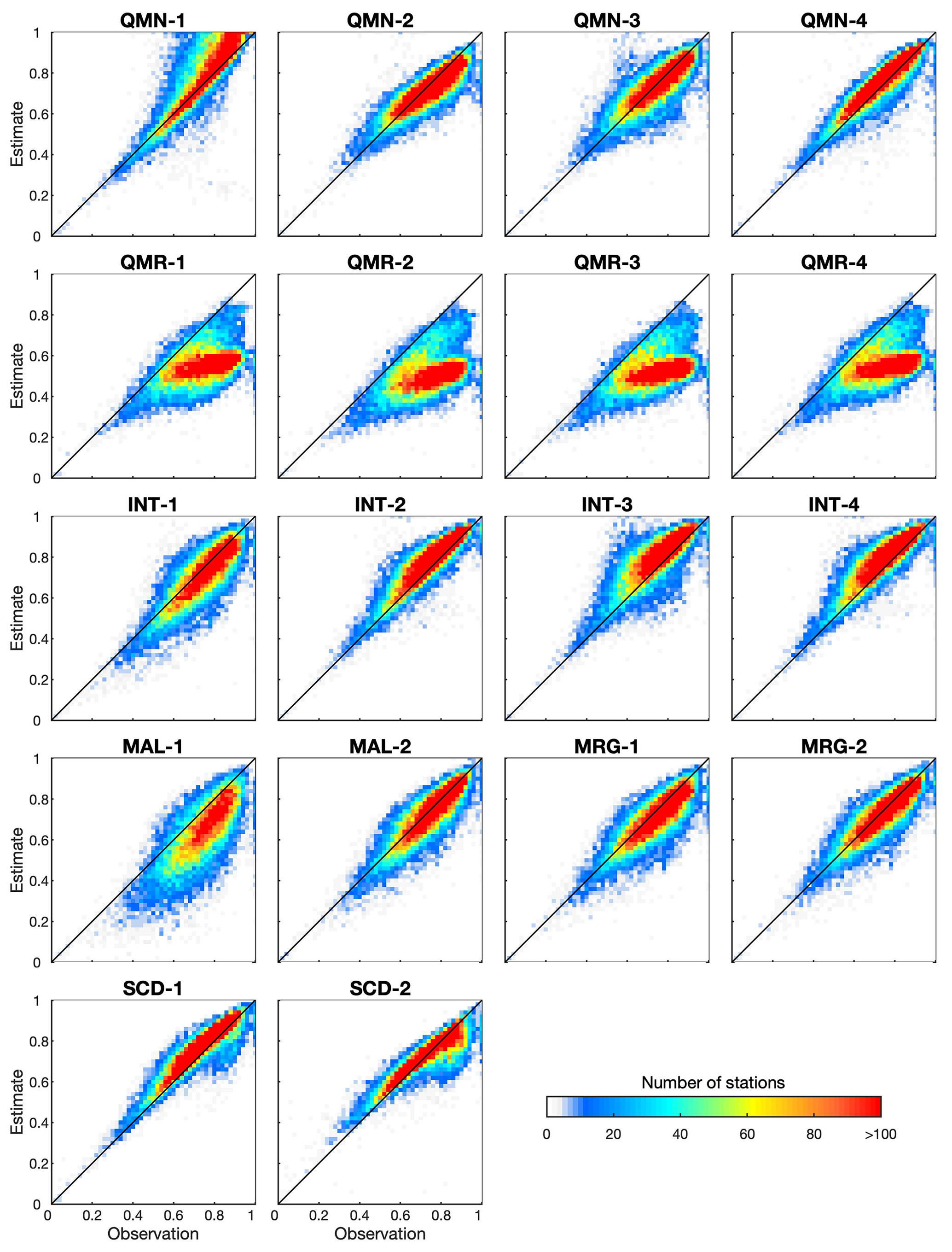
Figure 9Scatter density plots of CCs between precipitation from the target station and neighboring stations. For each target station, the neighboring station with the highest correlation with the target station is selected. The x axis represents the CC between observed precipitation from target and neighboring stations. The y axis represents the CC between estimated precipitation from the target station and the observed precipitation from the neighboring station. Each panel corresponds to one strategy in Sect. 3.3.2. SCD-1 represents SCD estimates after correction, while SCD-2 replaces estimates with observations. The CC is calculated for the overlapping observation period between target and neighboring stations, and the only exception is SCD-2 which calculates the CC using precipitation from target and neighboring stations during the entire period.
The variability of observations and of the corrected and uncorrected SCDNA estimates (Step-7 in Sect. 3.3.3) is compared using the SD of the observation period (Fig. 11). The SD of uncorrected SCDNA precipitation is lower than that of observations, while after correction the SD agrees very well with observations. The mean values of SD are 7.36, 6.30, and 7.36 for observations, uncorrected SCDNA, and corrected SCDNA, respectively. For Tmin and Tmax, corrected and uncorrected SCDNA estimates both show consistent variability to observations.

Figure 11The SD of observations and SCDNA estimates before and after correction. Data from the observation period are used.
4.3 The performance of the serially complete dataset
Uncorrected SCDNA estimates show high accuracy in North America (Fig. 12). For precipitation, the median KGE′ of all stations is 0.87, and the median values of r, β, and γ are 0.91, 0.92, and 0.96, respectively. The KGE′ for Mexican stations generally ranges between 0.6 and 0.8, which is smaller than that in the US and southern Canada. Some stations in the Rocky Mountains, the Caribbean, Alaska, and northern Canada (regions with complex topography or climate) also show lower KGE′ for precipitation estimates. The spatial distribution of r is similar to that of KGE′, while the magnitude is higher. According to γ, most stations underestimate precipitation variability, which is consistent with Fig. 11; β is generally lower than 1 in most regions of North America, particularly in the Rocky Mountains and Mexico where SCDNA underestimates precipitation.
Estimated temperature shows much higher KGE′ compared to precipitation. The median KGE′ and r of Tmin are 0.97 and 0.99, respectively. For Tmax, the median of KGE′ and r are 0.99 and 0.99, respectively. The median γ and β are both between 0.99 and 1 for Tmin and Tmax with small variations, particularly for Tmax (Fig. 12); the KGE′ of Tmin and Tmax is lower in the Caribbean and Mexico. For Tmin, the KGE′ for some stations around 45∘ N and the Rocky Mountains is lower than surrounding regions, although γ is spatially homogeneous for the same region. This is because the mean Tmin is close to 0 for some stations in this region, resulting in the large magnitude of β and γ. In contrast, Tmax exhibits homogeneous performance in the same region for all metrics.
Corrected SCDNA estimates (see Step-7 in Sect. 3.3.3 and Fig. S9 in the Supplement) have higher accuracy than uncorrected estimates (Fig. 12). For example, the median KGE′ for precipitation is improved from 0.87 to 0.90 after correction. The KGE′ for Tmin and Tmax is also improved but not as significantly as precipitation. The value of β equals 1 for all stations due to the mean value correction. For precipitation, γ changes from negative to positive for all stations, whereas the magnitude of the bias (deviation from 1) is smaller after correction. As a result, the spatial distribution of metrics for Tmin is also more homogeneous.
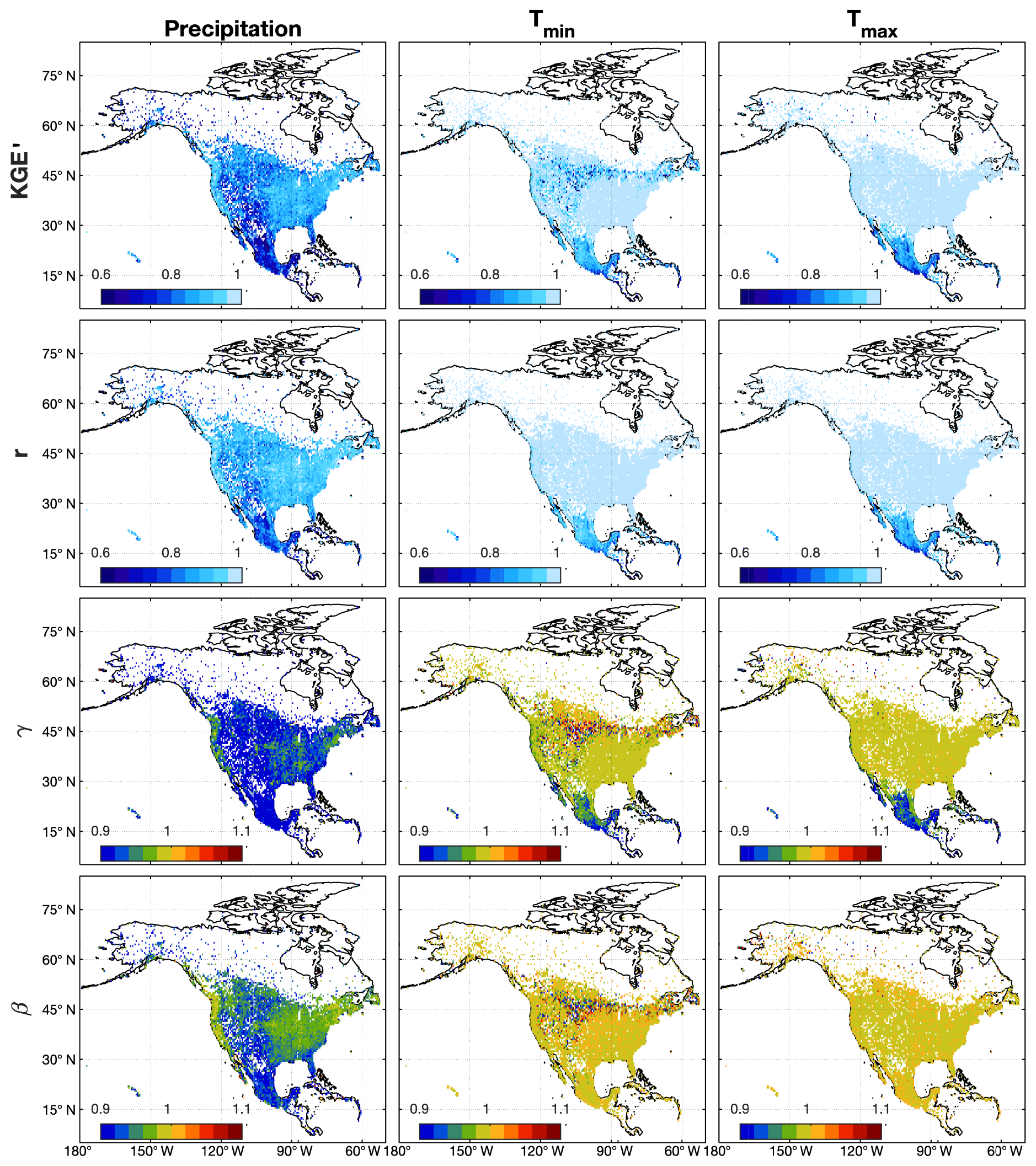
Figure 12The spatial distributions of KGE′ and its three components (r is the CC, β is the bias ratio, and γ is the variability ratio) for uncorrected SCDNA estimates over North America during the observation period. The maps are at a resolution of 0.5∘. The value for each grid cell is the median value of all stations within this grid cell.
The distributions of KGE′ vary during the year (Fig. 13). For precipitation, more stations show lower KGE′ during summer (DOY 150 to 250) than at other times of the year, which may be due to the variability of summertime convective precipitation. For Tmin, some stations show lower KGE′ from DOY 100 to 250. The seasonal variation of KGE′ for Tmax is relatively weak, although KGE′ is slightly more concentrated at a higher level during spring and autumn than winter and summer. The overall performance of Tmax is better than Tmin and precipitation.
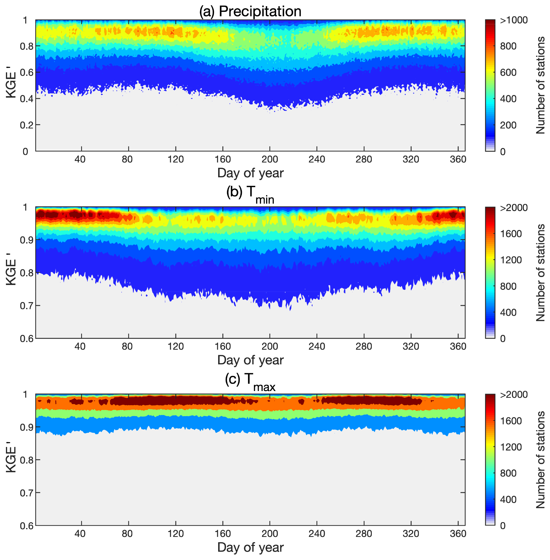
Figure 13The distribution of KGE′ for each day of the year for (a) precipitation, (b) Tmin, and (c) Tmax. Corrected SCDNA estimates are used.
4.4 Comparison between the serially complete dataset and gridded products
SCDNA precipitation and temperature are compared with benchmark gridded products to demonstrate whether the SCDNA is a good choice when station data are unavailable. Actual station observations are used as reference. Although assessing gridded products using point-scale station data contains uncertainties (Tang et al., 2018a), the objective of this section is to illustrate their agreement with station observations in lieu of providing an exhaustive quantitative assessment of their real-world accuracy.
Overall, the SCDNA achieves much higher KGE′ than reanalysis products for all variables (Fig. 14). For precipitation, the median KGE′ differences between the SCDNA and ERA5, JRA-55, and MERRA-2 are 0.48, 0.57, and 0.54, respectively. The corresponding KGE′ differences for Tmin are 0.46, 0.61, and 0.36, respectively. The improvement for Tmax is smaller, particularly in the eastern US where the topography is relatively flatter compared to the western US. The KGE′ differences of Tmean are lower than Tmin but higher than Tmax due to the offset effect. Trange suffers little from the elevation differences between stations and reanalysis grids and is suitable to demonstrate the differences between SCDNA and reanalysis products. The median KGE′ differences for Trange between the SCDNA and ERA5, JRA-55, and MERRA-2 are 0.31, 0.48, and 0.31, respectively.
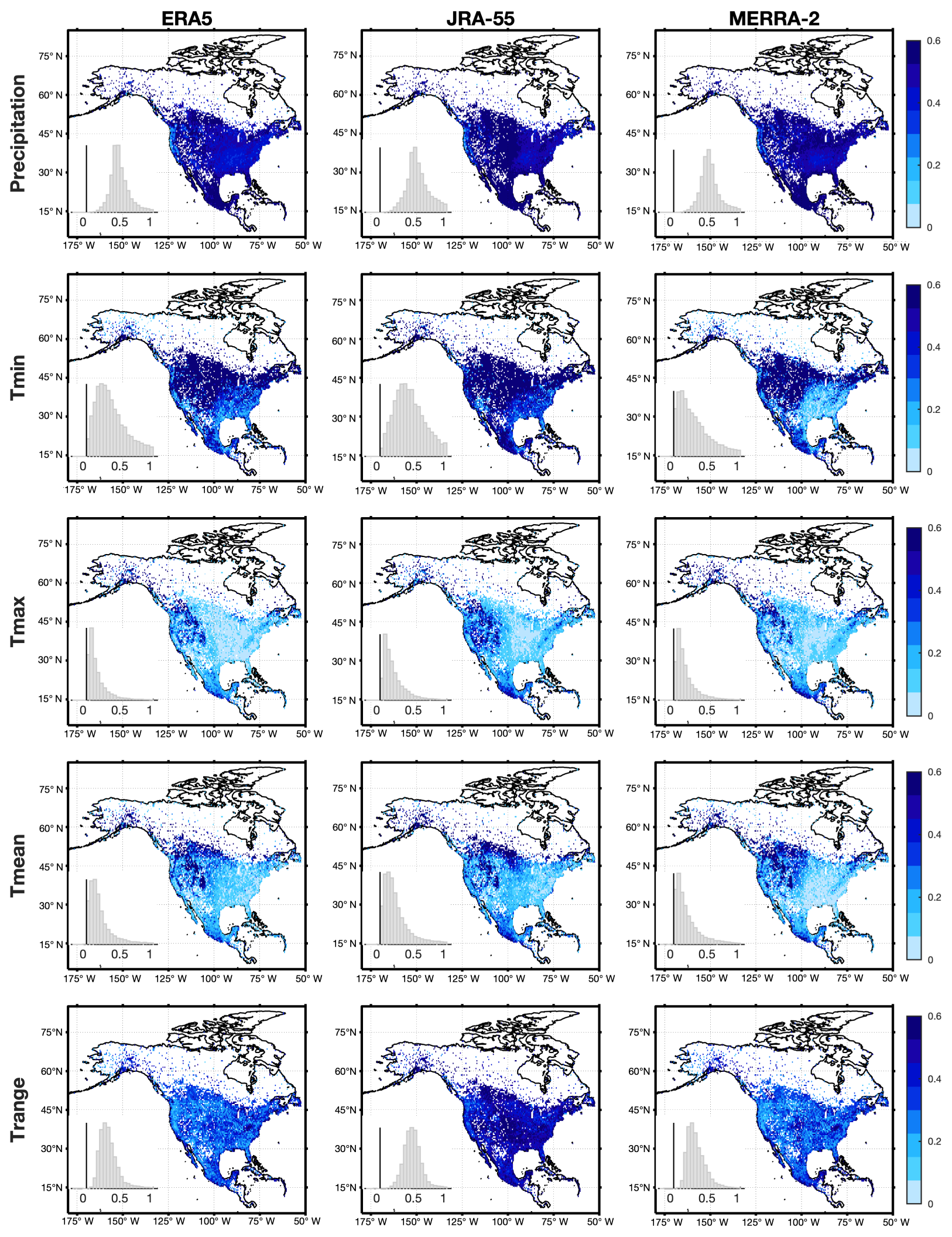
Figure 14Spatial distributions of KGE′ differences between SCDNA estimates and three reanalysis products (ERA5, JRA-55, and MERRA-2). The nested histograms show KGE′ differences between the SCDNA and reanalysis products. Corrected SCDNA estimates are used.
SCDNA and MSWEP precipitation is compared (Fig. 15). Since MSWEP merges data from numerous stations, the evaluation of MSWEP based on station data is not independent, which could result in the overestimation of its KGE′. Even so, SCDNA precipitation shows higher KGE′ than MSWEP for 98.97 % of stations with a median KGE′ difference of 0.31. Figure 15 shows notable differences between MSWEP and SCDNA at the Canada–US border and the US–Mexico border. This is because MSWEP infers gauge reporting times by searching for the highest correlation between gauge data and the temporally shifted reanalysis/satellite estimates (Beck et al., 2019). The estimated temporal shift could vary with countries, which results in distinct differences of station-based evaluation results along national boundaries. The accumulation periods of station and MSWEP precipitation are inconsistent in some cases, which could affect the evaluation of MSWEP (see Sect. 5.1).
Note that the evaluation does not indicate that the SCDNA has higher accuracy than the gridded products; rather, the results show that SCDNA is a better substitute than gridded products when station observations are unavailable.

Figure 15Spatial distributions of KGE′ differences between SCDNA and MSWEP precipitation. Corrected SCDNA estimates are used.
5.1 Observation time of stations
Meteorological stations in different countries usually have different local observation times, and stations in the same country may also experience changes in observation time (Vincent et al., 2012). Most station databases including those used in this study do not account for reporting time inconsistencies due to lack of hourly observations and well-documented station metadata. Vincent et al. (2009) examined several methods to adjust the time of daily precipitation observations, which, however, often altered observed precipitation intensity. Beck et al. (2019) inferred the reporting time of daily precipitation observations by calculating the SCC between the series of stations and gridded products, which is useful to correct the bias of gridded products. A simple experiment is carried out using the method of Beck et al. (2019) to infer the lag day of station series. For precipitation, 6418 stations show a non-negligible time shift from the reporting date (Fig. S10 in the Supplement). However, this method may be unsuitable for temperature because the estimated lag day is mostly zero, and the inferred reporting time cannot be directly applied to adjust station observations.
The inconsistent reporting time has different impacts on precipitation, Tmin, and Tmax. For example, if a station records data from 08:00 on 1 January to 08:00 on 2 January, the station will probably use 2 January as the reporting time. However, two-thirds of the 24 h time is on 1 January, indicating that the accumulated precipitation could mostly occur on 1 January. Tmax could also occur during the daytime on 1 January, but it is hard to determine on which day Tmin occurs, which makes it challenging to adjust precipitation, Tmin, and Tmax at the same time. The difference between universal and local time makes this problem more complicated. Thus, the reporting time of stations is not corrected here due to aforementioned difficulties.
5.2 Homogenization
Inhomogeneities in station observations are defined as variations that are not caused by weather and climate factors. Long-term station records are often subjected to inhomogeneities due to factors like station relocation, observation time change, instrument change, and surrounding environment change (Venema et al., 2012). Many methods have been developed to identify breakpoints and homogenize station series at annual, monthly, or even daily scales (e.g., Ma et al., 2008; Vincent et al., 2002, 2012). Different methods could generate different estimates of inhomogeneities as shown by many comparison studies (e.g., Beaulieu et al., 2008; Reeves et al., 2007; Venema et al., 2012). The four station databases (Sect. 2.1) used in this study provide original station records without homogenization. The SCDNA would inherit the potential inhomogeneities contained in these databases, and the infilling/reconstruction may also lead to discontinuities. The homogenization of the SCDNA is challenging considering that (1) the dataset covers a broad range of climate, topography, and countries, (2) the number of stations is large and differences between station periods (ranging from 8 to 40 years) are substantial, and (3) the suitability of existing methods for the homogenization of infilling/reconstruction estimates needs exploration. Therefore, homogenization is not carried out in this study, which, however, is an important direction for future studies.
5.3 Limitations of the KGE′ statistic
We use KGE′ because it incorporates information about correlation, bias, and variability and hence provides more information on methodological performance than an individual metric. For example, the PCC between temperature estimates and observations is usually close to 1 and cannot reflect the bias term, while the mean square error is prone to the effect of extreme values (or outliers). However, KGE′ also has limitations. For example, the values of KGE′ depend on the units of measurement (e.g., Santos et al., 2018) – in our case, the β values for temperature are clearly always close to 1 if the units of measurement for temperature are in Kelvin. Since these statistics incorrectly indicate very small temperature biases, we used degrees (∘) for all KGE′ calculations in this study, ensuring that β has more leverage in the KGE′ statistics. Moreover, and critical to our analysis, the normalization used in the KGE′ formula (β and γ) means that the KGE′ values are low when the denominators of β and γ are close to 0 (e.g., Santos et al., 2018). This problem is especially acute for temperature – for instance, we found that KGE′ values were very small for cases when μo is close to 0. Nevertheless, the number of cases where μo is close to 0 is rather small, where ∼0.5 % of all cases (based on all stations and all DOY) show absolute values of mean Tmin smaller than 0.1∘. For cases with μo close to 0, the ranking based on KGE′ is similar to the ranking based on mean absolute error, which means that KGE′ can still function as a ranking indicator when its value is low. Further work is needed to both comprehensively evaluate the alternative infilling strategies presented in this paper and evaluate more advanced multi-method merging strategies.
5.4 Potential improvement directions
Several steps could be taken to improve the SCDNA. First, the optimal strategy could be different for each station as shown in the results in this study. Therefore, the quality of SCDNA may be further improved by using more infilling/reconstruction methods, which would yield diminishing returns at some point. For example, the long short-term memory (LSTM) could be suitable for providing missing station observations. Optimizing the configuration of various strategies will be necessary to balance computation efficiency and estimation accuracy, particularly when the number of stations is large. Second, some stations suffer from undercatch, which depends on gauge type, precipitation phase, environmental conditions, etc. The bias caused by undercatch can be substantial for stations located at high latitudes and the mountains (Yang et al., 2005; Scaff et al., 2015). Third, the SCDNA does not distinguish between rainfall and snowfall. Considering that a large part of North America has frequent snowfall in winter, precipitation phase classification will be useful for hydrometeorological studies. Auxiliary data from reanalysis and satellite products could be used to partition precipitation into rain and snow. Finally, although the SCDNA agrees well with station observations, long-term trends are difficult to reconstruct when actual observations are unavailable, meaning the SCDNA may not be suitable for climate trend analysis in the reconstruction period. Some gridded datasets use only stations with long-term records (e.g., Wood, 2008; Werner et al., 2019) to achieve temporally consistent estimates, whereas such stations are very few. Reasonable trend estimation is challenging but meaningful for SCD.
Furthermore, other variables such as wind and humidity observed by stations also suffer from the same problems faced by precipitation and temperature. Future studies should explore whether the current methodology is applicable to other variables. An SCD covering more variables would be useful for research in various fields.
The SCDNA dataset is available at https://doi.org/10.5281/zenodo.3735533 (Tang et al., 2020) in netCDF format. The basic variables are station identification, latitude, longitude, elevation, date, and TLR derived in Sect. 3.2. Stations that undergo location merging (Sect. 3.1.1) are identified, and all relevant stations are included in the data file. For precipitation, Tmin, and Tmax, the variables in the netCDF4 file include original station observations, quality flags provided by original station databases, quality flags provided by this study, estimates from 16 strategies, uncorrected SCDNA estimates, corrected SCDNA estimates, the final SCDNA with estimates replaced by observations, data source flags indicating the source of each record in SCDNA (observations or 16 strategies), and accuracy metrics (KGE′ and its three components) for all estimates (16 strategies and SCDNA).
Scripts used to produce the SCDNA are available at https://github.com/tgq14/GapFill (last access: 21 July 2020). The dataset will be regularly updated to cover the latest periods.
This study developed a daily SCD of precipitation, Tmin, and Tmax for 27 276 stations from 1979 to 2018 over North America (SCDNA). The original station data are compiled from multiple sources and undergo strict quality control. Many stations have non-negligible fractions of missing values in the observation and reconstruction periods. For each station, the infilling and reconstruction are implemented using 16 strategies (quantile mapping, statistical interpolation, and machine learning) based on information from neighboring stations and concurrent reanalysis estimates (ERA5, JRA-55, and MERRA-2). The final SCDNA combines estimates from the 16 strategies and is corrected using station observations. The spatial correlation is preserved and might be slightly inflated. The SCDNA estimates reproduce the variance of original station observations very well, particularly for temperature. The median KGE′ of the final precipitation, Tmin, and Tmax for all stations is 0.90, 0.98, and 0.99, respectively. The comparison with four benchmark gridded products shows that the SCDNA has much better agreement with station observations. The SCDNA will be useful for a variety of hydrometeorological studies in North America.
Five types of checks (Durre et al., 2010) are adopted for the quality control of temperature.
-
Integrity checks. The first type of integrity check is a duplication check to identify duplicated records for time series in different time periods. The second type of integrity check includes the streak check to identify consecutive identical values and the frequent-value check to identify close but not necessarily consecutive identical values. The world record exceedance check sets lower (−89.4 ∘C) and upper (57.7 ∘C) bounds of temperature.
-
Outlier checks. These include the gap check that examines the frequency distributions for all calendar months and the climatological outlier check that is based on the traditional z score (e.g., Hubbard and You, 2005).
-
Internal and temporal consistency checks, including the iterative temperature consistency check. These ensure some inherent relationships are abided (e.g., Tmin cannot be larger than Tmax). The spike/dip check identifies temperatures which deviate from previous and following days by at least 25∘. The lagged temperature range check identifies abnormally large differences between Tmin and Tmax during a 3 d time window.
-
Spatial consistency checks, including the regression check and the spatial corroboration check. The regression check builds regression relationships between temperature at the target location and selected nearby stations to determine whether temperature at the target station should be flagged according to regression residuals and standardized residuals. The spatial corroboration check flags temperature at the target station if the value deviates far from the temperature at neighboring stations.
-
Extreme mega consistency checks. These ensure that certain relationships hold for the entire record of stations. For example, Tmax cannot be higher than the lowest Tmin for the calendar month, and vice versa.
For precipitation, quality control strategies are from three studies. The first part is similar to temperature but does not include the third type of checks (internal and temporal consistency checks). The second part is from Hamada et al. (2011).
-
Repetition checks. The nonzero check identifies constant daily values () that occur for more than 4 d. The zero check compares the annual zero-precipitation frequency with its climatological value to spot unusual frequencies of zero.
-
Duplicated monthly or sub-monthly record check. The temporal CC and the number of days with equal precipitation are used to identify whether 2 different months have the same records caused by human errors.
-
Z-score-based outlier check. Daily precipitation is flagged if its difference with the mean value from precipitation within a 15 d window of all years is larger than 9 SDs. This step is repeated until no outlier is identified.
-
Spatiotemporally isolated value check. Extremely large precipitation is identified in both space and time based on the percentiles of precipitation differences between the target station and neighboring stations within a radius of 400 km.
The third part is from Beck et al. (2019).
-
The empirical criterion is based on the fraction of days without precipitation (fD). This was designed to identify the long series of erroneous zero precipitation contained in GSOD station records. However, we found that this criterion misidentifies some acceptable records in GHCN-D. Therefore, the fD-based check is only implemented for GSOD.
-
Stations with fewer than 15 unique values or more than 99.5 % dry records (< 0.5 mm d−1) are discarded.
The supplement related to this article is available online at: https://doi.org/10.5194/essd-12-2381-2020-supplement.
GT and MC designed the study. GT collected data, performed the analyses, and wrote the paper. AN and AW helped design the framework and collect part of the data of the original databases. SP and VV helped determine the methodology and perform analysis on results. PW contributed to the design of infilling strategies and evaluation of the dataset. All authors contributed to data analysis, discussions about the methods and results, and paper improvement.
The authors declare that they have no conflict of interest.
The authors appreciate the extensive efforts from the developers of the ground and reanalysis datasets to make their products available. We thank chief editor Jens Klump and topical editor Scott Stevens for the handling of this paper and two anonymous referees for providing helpful feedback on the paper. The authors also thank Zenodo (https://zenodo.org/, last access: 29 September 2020) for publishing our dataset as open access to users.
This research has been supported by the Canada First Research Excellence Fund (Global Water Futures).
This paper was edited by Scott Stevens and reviewed by two anonymous referees.
Alexander, L. V., Zhang, X., Peterson, T. C., Caesar, J., Gleason, B., Tank, A. M. G. K., Haylock, M., Collins, D., Trewin, B., Rahimzadeh, F., Tagipour, A., Kumar, K. R., Revadekar, J., Griffiths, G., Vincent, L., Stephenson, D. B., Burn, J., Aguilar, E., Brunet, M., Taylor, M., New, M., Zhai, P., Rusticucci, M., and Vazquez-Aguirre, J. L.: Global observed changes in daily climate extremes of temperature and precipitation, J. Geophys. Res.-Atmos., 111, D05109, https://doi.org/10.1029/2005JD006290, 2006.
Anderson, B. T., Wang, J., Salvucci, G., Gopal, S., and Islam, S.: Observed Trends in Summertime Precipitation over the Southwestern United States, J. Climate, 23, 1937–1944, https://doi.org/10.1175/2009JCLI3317.1, 2009.
Beaulieu, C., Seidou, O., Ouarda, T. B. M. J., Zhang, X., Boulet, G., and Yagouti, A.: Intercomparison of homogenization techniques for precipitation data, Water Resour. Res., 44, W02425, https://doi.org/10.1029/2006WR005615, 2008.
Beck, H. E., van Dijk, A. I. J. M., Levizzani, V., Schellekens, J., Miralles, D. G., Martens, B., and de Roo, A.: MSWEP: 3-hourly 0.25∘ global gridded precipitation (1979–2015) by merging gauge, satellite, and reanalysis data, Hydrol. Earth Syst. Sci., 21, 589–615, https://doi.org/10.5194/hess-21-589-2017, 2017.
Beck, H. E., Wood, E. F., Pan, M., Fisher, C. K., Miralles, D. G., van Dijk, A. I. J. M., McVicar, T. R., and Adler, R. F.: MSWEP V2 Global 3-Hourly 0.1∘ Precipitation: Methodology and Quantitative Assessment, B. Am. Meteorol. Soc., 100, 473–500, https://doi.org/10.1175/BAMS-D-17-0138.1, 2019.
Breiman, L.: Random Forests, Mach. Learn., 45, 5–32, https://doi.org/10.1023/A:1010933404324, 2001.
Cannon, A. J., Sobie, S. R., and Murdock, T. Q.: Bias Correction of GCM Precipitation by Quantile Mapping: How Well Do Methods Preserve Changes in Quantiles and Extremes?, J. Climate, 28, 6938–6959, https://doi.org/10.1175/JCLI-D-14-00754.1, 2015.
Che Ghani, N. Z., Abu Hasan, Z., and Tze Liang, L.: Estimation of Missing Rainfall Data Using GEP: Case Study of Raja River, Alor Setar, Kedah, Adv. Artif. Intell., 2014, 716398, https://doi.org/10.1155/2014/716398, 2014.
Copernicus Climate Change Service (C3S): ERA5: Fifth generation of ECMWF atmospheric reanalyses of the global climate, Copernic. Clim. Change Serv. Clim. Data Store CDS Access Date July 2019, available at: https://cds.climate.copernicus.eu/cdsapp{#}!/home (last access: 19 October 2019), 2017.
Coulibaly, P. and Evora, N. D.: Comparison of neural network methods for infilling missing daily weather records, J. Hydrol., 341, 27–41, https://doi.org/10.1016/j.jhydrol.2007.04.020, 2007.
Dastorani, M. T., Moghadamnia, A., Piri, J., and Rico-Ramirez, M.: Application of ANN and ANFIS models for reconstructing missing flow data, Environ. Monit. Assess., 166, 421–434, https://doi.org/10.1007/s10661-009-1012-8, 2010.
Devi, U., Shekhar, M. S., Singh, G. P., Rao, N. N., and Bhatt, U. S.: Methodological application of quantile mapping to generate precipitation data over Northwest Himalaya, Int. J. Climatol., 39, 3160–3170, https://doi.org/10.1002/joc.6008, 2019.
Devine, K. A. and Mekis, E.: Field accuracy of Canadian rain measurements, Atmos.-Ocean, 46, 213–227, 2008.
Di Luzio, M., Johnson, G. L., Daly, C., Eischeid, J. K., and Arnold, J. G.: Constructing Retrospective Gridded Daily Precipitation and Temperature Datasets for the Conterminous United States, J. Appl. Meteorol. Climatol., 47, 475–497, https://doi.org/10.1175/2007JAMC1356.1, 2008.
Di Piazza, A., Conti, F. L., Noto, L. V., Viola, F., and La Loggia, G.: Comparative analysis of different techniques for spatial interpolation of rainfall data to create a serially complete monthly time series of precipitation for Sicily, Italy, Int. J. Appl. Earth Obs. Geoinf., 13, 396–408, https://doi.org/10.1016/j.jag.2011.01.005, 2011.
Durre, I., Menne, M. J., Gleason, B. E., Houston, T. G., and Vose, R. S.: Comprehensive Automated Quality Assurance of Daily Surface Observations, J. Appl. Meteorol. Climatol., 49, 1615–1633, https://doi.org/10.1175/2010JAMC2375.1, 2010.
Eischeid, J. K., Bruce Baker, C., Karl, T. R., and Diaz, H. F.: The Quality Control of Long-Term Climatological Data Using Objective Data Analysis, J. Appl. Meteorol., 34, 2787–2795, https://doi.org/10.1175/1520-0450(1995)034<2787:TQCOLT>2.0.CO;2, 1995.
Eischeid, J. K., Pasteris, P. A., Diaz, H. F., Plantico, M. S., and Lott, N. J.: Creating a Serially Complete, National Daily Time Series of Temperature and Precipitation for the Western United States, J. Appl. Meteorol., 39, 1580–1591, https://doi.org/10.1175/1520-0450(2000)039<1580:CASCND>2.0.CO;2, 2000.
Gao, L., Bernhardt, M., and Schulz, K.: Elevation correction of ERA-Interim temperature data in complex terrain, Hydrol. Earth Syst. Sci., 16, 4661–4673, https://doi.org/10.5194/hess-16-4661-2012, 2012.
Gao, L., Wei, J., Wang, L., Bernhardt, M., Schulz, K., and Chen, X.: A high-resolution air temperature data set for the Chinese Tian Shan in 1979–2016, Earth Syst. Sci. Data, 10, 2097–2114, https://doi.org/10.5194/essd-10-2097-2018, 2018.
Gardner, A. S., Sharp, M. J., Koerner, R. M., Labine, C., Boon, S., Marshall, S. J., Burgess, D. O., and Lewis, D.: Near-Surface Temperature Lapse Rates over Arctic Glaciers and Their Implications for Temperature Downscaling, J. Climate, 22, 4281–4298, https://doi.org/10.1175/2009jcli2845.1, 2009.
Gelaro, R., McCarty, W., Suárez, M. J., Todling, R., Molod, A., Takacs, L., Randles, C. A., Darmenov, A., Bosilovich, M. G., Reichle, R., Wargan, K., Coy, L., Cullather, R., Draper, C., Akella, S., Buchard, V., Conaty, A., da Silva, A. M., Gu, W., Kim, G.-K., Koster, R., Lucchesi, R., Merkova, D., Nielsen, J. E., Partyka, G., Pawson, S., Putman, W., Rienecker, M., Schubert, S. D., Sienkiewicz, M., and Zhao, B.: The Modern-Era Retrospective Analysis for Research and Applications, Version 2 (MERRA-2), J. Climate, 30, 5419–5454, https://doi.org/10.1175/jcli-d-16-0758.1, 2017.
Gruber, S.: Derivation and analysis of a high-resolution estimate of global permafrost zonation, The Cryosphere, 6, 221–233, https://doi.org/10.5194/tc-6-221-2012, 2012.
Gupta, H. V., Kling, H., Yilmaz, K. K., and Martinez, G. F.: Decomposition of the mean squared error and NSE performance criteria: Implications for improving hydrological modelling, J. Hydrol., 377, 80–91, 2009.
Hamada, A., Arakawa, O., and Yatagai, A.: An Automated Quality Control Method for Daily Rain-gauge Data, Glob. Environ. Res., 15, 183–192, 2011.
Hasanpour Kashani, M., and Dinpashoh, Y.: Evaluation of efficiency of different estimation methods for missing climatological data, Stoch. Environ. Res. Risk Assess., 26, 59–71, https://doi.org/10.1007/s00477-011-0536-y, 2012.
Hubbard, K. G. and You, J.: Sensitivity Analysis of Quality Assurance Using the Spatial Regression Approach—A Case Study of the Maximum/Minimum Air Temperature, J. Atmospheric Ocean. Technol., 22, 1520–1530, https://doi.org/10.1175/JTECH1790.1, 2005.
Kanda, N., Negi, H. S., Rishi, M. S., and Shekhar, M. S.: Performance of various techniques in estimating missing climatological data over snowbound mountainous areas of Karakoram Himalaya, Meteorol. Appl., 25, 337–349, https://doi.org/10.1002/met.1699, 2018.
Kemp, W. P., Burnell, D. G., Everson, D. O., and Thomson, A. J.: Estimating Missing Daily Maximum and Minimum Temperatures, J. Clim. Appl. Meteorol., 22, 1587–1593, https://doi.org/10.1175/1520-0450(1983)022<1587:EMDMAM>2.0.CO;2, 1983.
Kenawy, A. E., López-Moreno, J. I., Stepanek, P., and Vicente-Serrano, S. M.: An assessment of the role of homogenization protocol in the performance of daily temperature series and trends: application to northeastern Spain, Int. J. Climatol., 33, 87–108, https://doi.org/10.1002/joc.3410, 2013.
Kling, H., Fuchs, M., and Paulin, M.: Runoff conditions in the upper Danube basin under an ensemble of climate change scenarios, J. Hydrol., 424, 264–277, 2012.
Knowles, N., Dettinger, M. D., and Cayan, D. R.: Trends in Snowfall versus Rainfall in the Western United States, J. Climate, 19, 4545–4559, https://doi.org/10.1175/JCLI3850.1, 2006.
Kobayashi, S., Ota, Y., Harada, Y., Ebita, A., Moriya, M., Onoda, H., Onogi, K., Kamahori, H., Kobayashi, C., Endo, H., Miyaoka, K., and Takahashi, K.: The JRA-55 Reanalysis: General Specifications and Basic Characteristics, J. Meteorol. Soc. Jpn. Ser II, 93, 5–48, https://doi.org/10.2151/jmsj.2015-001, 2015.
Livneh, B., Bohn, T. J., Pierce, D. W., Munoz-Arriola, F., Nijssen, B., Vose, R., Cayan, D. R., and Brekke, L.: A spatially comprehensive, hydrometeorological data set for Mexico, the U.S., and Southern Canada 1950–2013, Sci. Data, 2, 150042, https://doi.org/10.1038/sdata.2015.42, 2015.
Longman, R. J., Frazier, A. G., Newman, A. J., Giambelluca, T. W., Schanzenbach, D., Kagawa-Viviani, A., Needham, H., Arnold, J. R., and Clark, M. P.: High-Resolution Gridded Daily Rainfall and Temperature for the Hawaiian Islands (1990–2014), J. Hydrometeorol., 20, 489–508, https://doi.org/10.1175/JHM-D-18-0112.1, 2019.
Longman, R. J., Newman, A. J., Giambelluca, T. W., and Lucas, M.: Characterizing the Uncertainty and Assessing the Value of Gap-Filled Daily Rainfall Data in Hawaii, J. Appl. Meteorol. Climatol., 59, 1261–1276, https://doi.org/10.1175/JAMC-D-20-0007.1, 2020.
Ma, C., Fassnacht, S. R., and Kampf, S. K.: How Temperature Sensor Change Affects Warming Trends and Modeling: An Evaluation Across the State of Colorado, Water Resour. Res., 55, 9748–9764, 2019.
Ma, L., Zhang, T., Li, Q., Frauenfeld, O. W., and Qin, D.: Evaluation of ERA-40, NCEP-1, and NCEP-2 reanalysis air temperatures with ground-based measurements in China, J. Geophys. Res., 113, D15115, https://doi.org/10.1029/2007jd009549, 2008.
Ma, Y., Hong, Y., Chen, Y., Yang, Y., Tang, G., Yao, Y., Long, D., Li, C., Han, Z., and Liu, R.: Performance of Optimally Merged Multisatellite Precipitation Products Using the Dynamic Bayesian Model Averaging Scheme Over the Tibetan Plateau, J. Geophys. Res.-Atmos., 123, 814–834, https://doi.org/10.1002/2017jd026648, 2018.
Maraun, D.: Bias Correction, Quantile Mapping, and Downscaling: Revisiting the Inflation Issue, J. Climate, 26, 2137–2143, https://doi.org/10.1175/JCLI-D-12-00821.1, 2013.
Marshall, S. J., Sharp, M. J., Burgess, D. O., and Anslow, F. S.: Near-surface-temperature lapse rates on the Prince of Wales Icefield, Ellesmere Island, Canada: implications for regional downscaling of temperature, Int. J. Climatol., 27, 385–398, https://doi.org/10.1002/joc.1396, 2007.
Mekis, É. and Brown, R.: Derivation of an adjustment factor map for the estimation of the water equivalent of snowfall from ruler measurements in Canada, Atmos.-Ocean, 48, 284–293, https://doi.org/10.3137/AO1104.2010, 2010.
Menne, M. J., Durre, I., Vose, R. S., Gleason, B. E., and Houston, T. G.: An overview of the global historical climatology network-daily database, J. Atmospheric Ocean. Technol., https://doi.org/10.1175/JTECH-D-11-00103.1, 2012.
Metcalfe, J. R., Routledge, B., and Devine, K.: Rainfall measurement in Canada: changing observational methodsand archive adjustment procedures, J. Climate, 10, 92–101, 1997.
Minder, J. R., Mote, P. W., and Lundquist, J. D.: Surface temperature lapse rates over complex terrain: Lessons from the Cascade Mountains, J. Geophys. Res.-Atmos., 115, D14122. https://doi.org/10.1029/2009JD013493, 2010.
Newman, A. J., Clark, M. P., Craig, J., Nijssen, B., Wood, A., Gutmann, E., Mizukami, N., Brekke, L., and Arnold, J. R.: Gridded Ensemble Precipitation and Temperature Estimates for the Contiguous United States, J. Hydrometeorol., 16, 2481–2500, https://doi.org/10.1175/JHM-D-15-0026.1, 2015.
Newman, A. J., Clark, M. P., Longman, R. J., Gilleland, E., Giambelluca, T. W., and Arnold, J. R.: Use of Daily Station Observations to Produce High-Resolution Gridded Probabilistic Precipitation and Temperature Time Series for the Hawaiian Islands, J. Hydrometeorol., 20, 509–529, https://doi.org/10.1175/JHM-D-18-0113.1, 2019.
Papalexiou, S. M. and Montanari, A.: Global and regional increase of precipitation extremes under global warming, Water Resour. Res., 55, 4901–4914, 2019.
Papalexiou, S. M., AghaKouchak, A., Trenberth, K. E., and Foufoula-Georgiou, E.: Global, regional, and megacity trends in the highest temperature of the year: Diagnostics and evidence for accelerating trends, Earths Future, 6, 71–79, 2018.
Pappas, C., Papalexiou, S. M., and Koutsoyiannis, D.: A quick gap filling of missing hydrometeorological data, J. Geophys. Res.-Atmos., 119, 9290–9300, 2014.
Paulhus, J. L. H. and Kohler, M. A.: Interpolation of missing precipitation records, Mon. Weather Rev., 80, 129–133, https://doi.org/10.1175/1520-0493(1952)080<0129:IOMPR>2.0.CO;2, 1952.
Pielke Sr, R., Nielsen-Gammon, J., Davey, C., Angel, J., Bliss, O., Doesken, N., Cai, M., Fall, S., Niyogi, D., and Gallo, K.: Documentation of uncertainties and biases associated with surface temperature measurement sites for climate change assessment, B. Am. Meteorol. Soc., 88, 913–928, 2007.
Ramos-Calzado, P., Gómez-Camacho, J., Pérez-Bernal, F., and Pita-López, M. F.: A novel approach to precipitation series completion in climatological datasets: application to Andalusia, Int. J. Climatol., 28, 1525–1534, https://doi.org/10.1002/joc.1657, 2008.
Reeves, J., Chen, J., Wang, X. L., Lund, R., and Lu, Q. Q.: A Review and Comparison of Changepoint Detection Techniques for Climate Data, J. Appl. Meteorol. Climatol., 46, 900–915, https://doi.org/10.1175/JAM2493.1, 2007.
Rubin, D. B.: Inference and missing data, Biometrika, 63, 581–592, https://doi.org/10.1093/biomet/63.3.581, 1976.
Santos, L., Thirel, G., and Perrin, C.: Technical note: Pitfalls in using log-transformed flows within the KGE criterion, Hydrol. Earth Syst. Sci., 22, 4583–4591, https://doi.org/10.5194/hess-22-4583-2018, 2018.
Sattari, M.-T., Rezazadeh-Joudi, A., and Kusiak, A.: Assessment of different methods for estimation of missing data in precipitation studies, Hydrol. Res., 48, 1032–1044, https://doi.org/10.2166/nh.2016.364, 2017.
Scaff, L., Yang, D., Li, Y., and Mekis, E.: Inconsistency in precipitation measurements across the Alaska–Yukon border, The Cryosphere, 9, 2417–2428, https://doi.org/10.5194/tc-9-2417-2015, 2015.
Serrano-Notivoli, R., Beguería, S., and de Luis, M.: STEAD: a high-resolution daily gridded temperature dataset for Spain, Earth Syst. Sci. Data, 11, 1171–1188, https://doi.org/10.5194/essd-11-1171-2019, 2019.
Shepard, D.: A two-dimensional interpolation function for irregularly-spaced data, in: Proceedings of the 1968 23rd ACM national conference, pp. 517–524, ACM, Association for Computing Machinery, New York, NY, United States, 1968.
Simolo, C., Brunetti, M., Maugeri, M., and Nanni, T.: Improving estimation of missing values in daily precipitation series by a probability density function-preserving approach, Int. J. Climatol., 30, 1564–1576, https://doi.org/10.1002/joc.1992, 2010.
Stooksbury, D. E., Idso, C. D., and Hubbard, K. G.: The Effects of Data Gaps on the Calculated Monthly Mean Maximum and Minimum Temperatures in the Continental United States: A Spatial and Temporal Study, J. Climate, 12, 1524–1533, https://doi.org/10.1175/1520-0442(1999)012<1524:TEODGO>2.0.CO;2, 1999.
Tang, G., Behrangi, A., Long, D., Li, C., and Hong, Y.: Accounting for spatiotemporal errors of gauges: A critical step to evaluate gridded precipitation products, J. Hydrol., 559, 294–306, https://doi.org/10.1016/j.jhydrol.2018.02.057, 2018a.
Tang, G., Behrangi, A., Ma, Z., Long, D., and Hong, Y.: Downscaling of ERA-Interim Temperature in the Contiguous United States and Its Implications for Rain–Snow Partitioning, J. Hydrometeorol., 19, 1215–1233, https://doi.org/10.1175/jhm-d-18-0041.1, 2018b.
Tang, G., Clark, M. P., Newman, A. J., Wood, A. W., Papalexiou, S. M., Vionnet, V., Whitfield, P. H.: SCDNA: a serially complete precipitation and temperature dataset for North America from 1979 to 2018, Zenodo, https://doi.org/10.5281/zenodo.3735533, 2020.
Tang, Q., Wood, A. W., and Lettenmaier, D. P.: Real-Time Precipitation Estimation Based on Index Station Percentiles, J. Hydrometeorol., 10, 266–277, https://doi.org/10.1175/2008JHM1017.1, 2009.
Teegavarapu, R. S. V. and Chandramouli, V.: Improved weighting methods, deterministic and stochastic data-driven models for estimation of missing precipitation records, J. Hydrol., 312, 191–206, https://doi.org/10.1016/j.jhydrol.2005.02.015, 2005.
Ustaoglu, B., Cigizoglu, H. K., and Karaca, M.: Forecast of daily mean, maximum and minimum temperature time series by three artificial neural network methods, Meteorol. Appl., 15, 431–445, https://doi.org/10.1002/met.83, 2008.
Venema, V. K. C., Mestre, O., Aguilar, E., Auer, I., Guijarro, J. A., Domonkos, P., Vertacnik, G., Szentimrey, T., Stepanek, P., Zahradnicek, P., Viarre, J., Müller-Westermeier, G., Lakatos, M., Williams, C. N., Menne, M. J., Lindau, R., Rasol, D., Rustemeier, E., Kolokythas, K., Marinova, T., Andresen, L., Acquaotta, F., Fratianni, S., Cheval, S., Klancar, M., Brunetti, M., Gruber, C., Prohom Duran, M., Likso, T., Esteban, P., and Brandsma, T.: Benchmarking homogenization algorithms for monthly data, Clim. Past, 8, 89–115, https://doi.org/10.5194/cp-8-89-2012, 2012.
Vicente-Serrano, S. M., Saz-Sanchez, M. A., and Cuadrat, J. M.: Comparative analysis of interpolation methods in the middle Ebro Valley (Spain): application to annual precipitation and temperature, Clim. Res., 24, 161–180, https://doi.org/10.3354/cr024161, 2003.
Vincent, L. A., Zhang, X., Bonsal, B. R., and Hogg, W. D.: Homogenization of Daily Temperatures over Canada, J. Climate, 15, 1322–1334, https://doi.org/10.1175/1520-0442(2002)015<1322:HODTOC>2.0.CO;2, 2002.
Vincent, L. A., Milewska, E. J., Hopkinson, R., and Malone, L.: Bias in Minimum Temperature Introduced by a Redefinition of the Climatological Day at the Canadian Synoptic Stations, J. Appl. Meteorol. Climatol., 48, 2160–2168, https://doi.org/10.1175/2009JAMC2191.1, 2009.
Vincent, L. A., Wang, X. L., Milewska, E. J., Wan, H., Yang, F., and Swail, V.: A second generation of homogenized Canadian monthly surface air temperature for climate trend analysis, J. Geophys. Res.-Atmos., 117, D18110, https://doi.org/10.1029/2012JD017859, 2012.
Wambua, R. M., Mutua, B. M., and Raude, J. M.: Prediction of Missing Hydro-Meteorological Data Series Using Artificial Neural Networks (ANN) for Upper Tana River Basin, Kenya, Am. J. Water Resour., 4, 35–43, , 2016.
Wang, X. L., Xu, H., Qian, B., Feng, Y., and Mekis, E.: Adjusted daily rainfall and snowfall data for Canada, Atmos.-Ocean, 55, 155–168, 2017.
Werner, A. T., Schnorbus, M. A., Shrestha, R. R., Cannon, A. J., Zwiers, F. W., Dayon, G., and Anslow, F.: A long-term, temporally consistent, gridded daily meteorological dataset for northwestern North America, Sci. Data, 6, 1–16, https://doi.org/10.1038/sdata.2018.299, 2019.
Whitfield, P. H.: Climate Station Analysis and Fitness for Purpose Assessment of 3053600 Kananaskis, Alberta, Atmos.-Ocean, 52, 363–383, https://doi.org/10.1080/07055900.2014.946388, 2014.
Woldesenbet, T. A., Elagib, N. A., Ribbe, L., and Heinrich, J.: Gap filling and homogenization of climatological datasets in the headwater region of the Upper Blue Nile Basin, Ethiopia, Int. J. Climatol., 37, 2122–2140, https://doi.org/10.1002/joc.4839, 2017.
Wood, A. W.: The University of Washington Surface Water Monitor: An experimental platform for national hydrologic assessment and prediction, in: Proceedings of the AMS 22nd Conference on Hydrology, New Orleans, Louisiana, USA, 2008.
Yamazaki, D., Ikeshima, D., Tawatari, R., Yamaguchi, T., O'Loughlin, F., Neal, J. C., Sampson, C. C., Kanae, S., and Bates, P. D.: A high-accuracy map of global terrain elevations, Geophys. Res. Lett., 44, 5844–5853, https://doi.org/10.1002/2017GL072874, 2017.
Yang, D., Kane, D., Zhang, Z., Legates, D., and Goodison, B.: Bias corrections of long-term (1973-2004) daily precipitation data over the northern regions, Geophys. Res. Lett., 32, L19501, https://doi.org/10.1029/2005gl024057, 2005.
Yatagai, A., Kamiguchi, K., Arakawa, O., Hamada, A., Yasutomi, N., and Kitoh, A.: APHRODITE: Constructing a Long-Term Daily Gridded Precipitation Dataset for Asia Based on a Dense Network of Rain Gauges, B. Am. Meteorol. Soc., 93, 1401–1415, https://doi.org/10.1175/bams-d-11-00122.1, 2012.
Young, K. C.: A Three-Way Model for Interpolating for Monthly Precipitation Values, Mon. Weather Rev., 120, 2561–2569, https://doi.org/10.1175/1520-0493(1992)120<2561:ATWMFI>2.0.CO;2, 1992.