the Creative Commons Attribution 4.0 License.
the Creative Commons Attribution 4.0 License.
 | 05 Feb 2020
Paleo-hydrologic reconstruction of 400 years of past flows at a weekly time step for major rivers of Western Canada
Andrew R. Slaughter
Saman Razavi
The assumption of stationarity in water resources no longer holds, particularly within the context of future climate change. Plausible scenarios of flows that fluctuate outside the envelope of variability of the gauging data are required to assess the robustness of water resource systems to future conditions. This study presents a novel method of generating weekly time step flows based on tree-ring chronology data. Specifically, this method addresses two long-standing challenges with paleo-reconstruction: (i) the typically limited predictive power of tree-ring data at the annual and sub-annual scale and (ii) the inflated short-term persistence in tree-ring time series and improper use of pre-whitening. Unlike the conventional approach, this method establishes relationships between tree-ring chronologies and naturalized flow at a biennial scale to preserve persistence properties and variability of hydrological time series. Biennial flow reconstructions are further disaggregated to weekly flow reconstructions, according to the weekly flow distribution of reference 2-year instrumental periods, identified as periods with broadly similar tree-ring properties to those of every 2-year paleo-period. The Saskatchewan River basin (SaskRB) in Western Canada is selected as a study area, and weekly flows in its four major tributaries are extended back to the year 1600. The study shows that the reconstructed flows properly preserve the statistical properties of the reference flows, particularly in terms of short- to long-term persistence and the structure of variability across timescales. An ensemble approach is presented to represent the uncertainty inherent in the statistical relationships and disaggregation method. The ensemble of reconstructed weekly flows are publicly available for download from https://doi.org/10.20383/101.0139 (Slaughter and Razavi, 2019).
- Article
(5804 KB) - Full-text XML
- BibTeX
- EndNote


Water management has traditionally assumed that variability in streamflow fluctuates within a boundary represented by the limited amount of observed data provided by gauging stations. This limited variability has been used to evaluate and manage risks to water management systems. However, it is becoming increasingly clear that the assumption of stationarity can no longer be taken for granted (Milly et al., 2008), particularly within the context of future climate change.
An opportunity exists to derive a paleo-hydrological record that will contain the effects of past climate change. Earth has always experienced strong climate change effects in the past, even in the absence of anthropogenic effects. Of course, these effects have been intensified in the Anthropocene; for example, refer to Cohn and Lins (2005) and Razavi et al. (2015). Reconstructions of flow from tree-ring records for various parts of the world have shown relatively high long-term variability in hydrologic conditions at the multi-decadal to multi-century temporal scale (Agafonov et al., 2016; Axelson et al., 2009; Boucher et al., 2011; Brigode et al., 2016; Case and MacDonald 2003; Cook et al., 2004; Ferrero et al., 2015; Gangopadhyay et al., 2009; Lara et al., 2015; Maxwell et al., 2011; Mokria et al., 2018; Razavi et al., 2015, 2016; Sauchyn et al., 2011; Urrutia et al., 2011; Woodborne et al., 2015; Woodhouse and Lukus, 2006; Woodhouse et al., 2006). Therefore, tree-ring records could provide an opportunity to evaluate water resource systems against a wider envelope of hydrological variability than what is represented in the gauged records. This is critical for improving the resilience of water resource systems to future conditions.
However, there are various challenges associated with the use of tree-ring data to reconstruct streamflows, as outlined by Razavi et al. (2016) and Elshorbagyet al. (2016), that add to the uncertainty of flow reconstructions, the most important being (1) tree-ring widths can only explain a portion of the variance in observed streamflow, and past studies correlating tree-ring chronologies to streamflow have obtained relatively low R2 values, with some values as low as 0.37 but some as high as 0.76 (Razavi et al., 2016), and (2) there is short-term persistence in tree-ring chronologies that is typically higher than that in observed streamflow. Pre-whitening techniques are commonly used to remove short-term persistence within chronology datasets. However, Razavi and Vogel (2018) found that pre-whitening can distort and reduce the structure of variability across timescales. A viable strategy of reducing the disparities in persistence between tree-ring chronologies and flow while at the same time increasing their correlative strength is to establish the statistical relationships at longer timescales of 2 to 3 years (Razavi et al., 2016; Razavi and Vogel, 2018).
Because water resources models require flow input data at daily to monthly time steps and flow reconstructions from tree-ring data are typically at a yearly time step, some kind of method of flow disaggregation is required. Although many studies have established relationships between tree-ring chronologies and flow at the annual scale, very few published studies have attempted to further disaggregate reconstructed flow. Sauchyn and Ilich (2017) estimated 900 years of weekly flows for the North Saskatchewan River at Edmonton and for the South Saskatchewan River at Medicine Hat. They determined the statistical relationships between tree-ring chronologies and mean annual naturalized flow using standard dendrohydrological techniques but further disaggregated yearly flows to weekly using stochastic downscaling while constraining the resulting weekly flows by the statistical properties of the historical record.
This study presents a novel approach for reconstructing flows from tree-ring data and disaggregating these flows to a weekly time step while taking into account reconstruction uncertainty through an ensemble approach. As a result, 400 years of weekly flows were generated for the four major sub-basins of the Saskatchewan River basin. The Saskatchewan River is a river of great ecological, social and economic importance in Western Canada. The approach of reconstructing flow from tree-ring chronologies contains multiple sources of uncertainty, including the choice of predictor chronologies and the choice of disaggregation technique (Razavi et al., 2016). The present study presents an ensemble approach for encompassing these uncertainties.
2.1 Case study
The Saskatchewan River basin (SaskRB) in Western Canada is a large river basin with an area of approximately 400 000 km2, which transcends Alberta, Saskatchewan and Manitoba provinces, and also extends into a small part of the American state of Montana (Fig. 1). The east-facing Rocky Mountains to the west, at over 3000 m in elevation, act as the “water tower” of the basin (Martz et al., 2007; Pomeroy et al., 2005), contributing up to 95 % of the total basin flow, after which the elevation of the basin drops to 750, 450 and 300 m on the plains of Alberta, Saskatchewan and Manitoba, respectively, transitioning from alpine forest to prairie grasslands and river valley forest. Long sunny winters and short hot summers characterize the climate of the basin, and there is a dramatic rainfall gradient from west to east, with precipitation of up to 1500 mm yr−1 in the mountains to 300–500 mm yr−1 on the semi-arid plains.
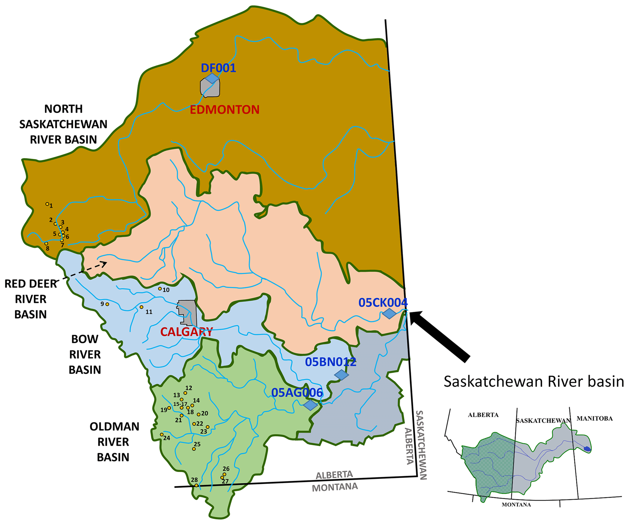
Figure 1Map (adapted from Razavi et al., 2016) of the tributaries of the Saskatchewan River basin and the locations of the chronology sites (circles) and streamflow gauges (diamonds).
2.2 Data
Tree-ring data for the major headwater tributaries of the SaskRB were used, namely the North Saskatchewan, Red Deer, Bow and Oldman rivers. Naturalized flows generated by Alberta Environment and Sustainable Resource Development for four gauging stations (1912–2001) representing each of the four headwater tributaries were used in the analysis (see Fig. 1). A total of 16 tree-ring chronology sites were used, with most from sites chosen for soil moisture availability only during snowmelt or rainfall. These chronology data were obtained from the Prairie Adaptation Research Collaborative (PARC; https://www.parc.ca/, last access: February 2020). Razavi et al. (2016) describe the tree-ring measurement, detrending and averaging procedures used. The tree-ring chronologies used represent tree growth rates from 1600 to 2001.
2.3 Methodology
2.3.1 Reconstruction of flows based on tree-ring chronologies
The traditional method of reconstructing streamflow based on tree-ring chronologies is through correlations between tree-ring chronologies and observed streamflow at the yearly scale. However, as shown by Razavi et al. (2016), there are stronger correlations between tree-ring chronologies and streamflow at multi-year timescales. In addition, establishing correlations at multi-year timescales can be a viable method of overcoming the significantly higher persistence in tree-ring chronologies compared to streamflow without resorting to pre-whitening techniques, which have been shown to result in a loss of information not related to autocorrelation (Razavi et al., 2016; Razavi and Vogel, 2017). The persistence present in tree-ring chronologies is due to a mixture of the persistence in the climate signal and the biological carry-over effects of trees, which, for example, would allow trees to tolerate a water shortage in a dry year if the preceding year was wet. In addition, teleconnection signals typically occur in concert with precipitation in a region and thus with water availability for tree growth. Therefore, tree-ring chronologies and their respective streamflow reconstructions should carry the teleconnection signals. As shown by Razavi et al. (2016), the persistence effect diminishes over a longer timescale. Although the relationship between streamflow and tree-ring chronologies strengthens at multi-year timescales, establishing this relationship at an optimal timescale that can be in the order of 5 years (Razavi et al., 2016) would disadvantage the process of disaggregation of reconstructed flow. Therefore, as a compromise, the present study established statistical relationships between 2-year moving averages of tree-ring chronologies and naturalized streamflows. Multiple linear regression (MLR) fitted by least squares was the statistical approach taken to establish the relationships between tree-ring chronologies and streamflows. We can expect a fairly linear relationship between flow and tree-ring growth, as observed in many regions of the world (Axelson et al., 2009; Boucher et al., 2011; Case and MacDonald, 2003; Gou et al., 2007; Souchyn and Ilich, 2017), and MLR is a simple but effective method of representing this direct monotonic (approximately linear) relationship between tree growth rate and flow. The predictive ability of the models was assessed through the coefficient of determination, R2. Similar to Razavi et al. (2016), since the North Saskatchewan River and Oldman River sub-basins contained sufficient chronology sites, only the four and eight chronology sites falling within the sub-basins, respectively, were used to establish their respective MLR models; whereas since few or no sites were present in the Red Deer River and Bow River sub-basins (Fig. 1), all 16 chronologies were used to establish their MLR models. Building on the experience of Razavi et al. (2016) and employing the Akaike Information Criterion, models using both three and two chronology predictors (tree-ring stations) were established for the North Saskatchewan River and Oldman River sub-basins, whereas MLR models with only two chronology predictors were established for Bow River and Red Deer River sub-basins. MLR models were generated for the shared period between tree-ring chronologies and naturalized streamflows of 1912–2001. A leave-one-out cross-validation strategy was used to test the performance of each model. This validation strategy maximizes our ability in validating the MLR models using the relatively short overlap period between the tree-ring chronologies and reference flow and provides a more accurate measure of model goodness of fit and can identify and avoid overfitting. To account for the uncertainty in streamflow reconstructions, multiple MLR models with the best performances were selected for each sub-basin. The choice of the best models for each sub-basin was rather subjective and depended on relative R2 values achieved for all the models generated.
2.3.2 Disaggregation of 2-year reconstructed flows to weekly flows
Although there are definite advantages to reconstructing streamflow from tree-ring chronologies at multi-year timescales (Razavi et al., 2016), the usefulness of these flows for evaluating water resource systems is limited. Generating weekly reconstructed streamflow would be of more use in evaluating water resource systems, for example, the established water management model, the Water Resources Management Model (WRMM) (Alberta Environment, 2002) used within the Prairie Provinces, runs on a weekly time step. The conceptual approach taken can be represented in Fig. 2. The basic premise adopted is that biennial reconstructed flow can be disaggregated to weekly reconstructed flow by the selection of biennial flow periods from the reference naturalized flow (1912–2001) (2-year instrumental periods) with similar attributes to the biennial reconstructed flow, after which the weekly flow distribution of the selected reference flow period can be used to construct the weekly flows. The attributes used to match the biennial reconstructed flow with biennial reference flow were hydrological condition, simply defined as dry, normal and wet conditions corresponding to flow lower than the 25th percentile, between the 25th percentile and the 75th percentile, and greater than the 75th percentile, respectively, and which year in each biennial flow, year 1 or year 2, contributes the greater amount of flow. In Fig. 2, (1) represents the average tree-ring growth rates of all the tree-ring chronologies used to generate a particular MLR model for a sub-basin on a yearly time step. By examining the yearly tree-ring growth rates in pairs (on a biennial scale), it can be determined which yearly growth rate, i.e. of year 1 or year 2, is larger. Since we constructed biennial flows from biennial tree-ring growth rates, this allows B for each biennial flow in (2) to be set to 1 or 2 to indicate whether the first or second year of that biennial flow value contributed the greater flow. In Fig. 2, “A” in (2) represents the hydrological condition explained earlier. A similar process is performed for the weekly naturalized reference flow in (3), except that average yearly flows are used to set “B”. The biennial reconstructed flow is then stepped through in (4), and a similar period according to A and B is randomly selected from the biennial reference flow. The approach of random matching allows an ensemble of weekly flow reconstructions to be generated for each single biennial flow reconstruction while retaining the same underlying statistical properties. The weekly distribution of flows in the selected biennial reference flow period is then used to construct the weekly flow reconstruction, scaled to have the same biennial average as the original reconstructed biennial flow. An argument could be made that the scaling should be according to the variance of the biennial reference flow; however, the variance of the reconstructed flow was found to be similar to that of the reference flow using this approach.
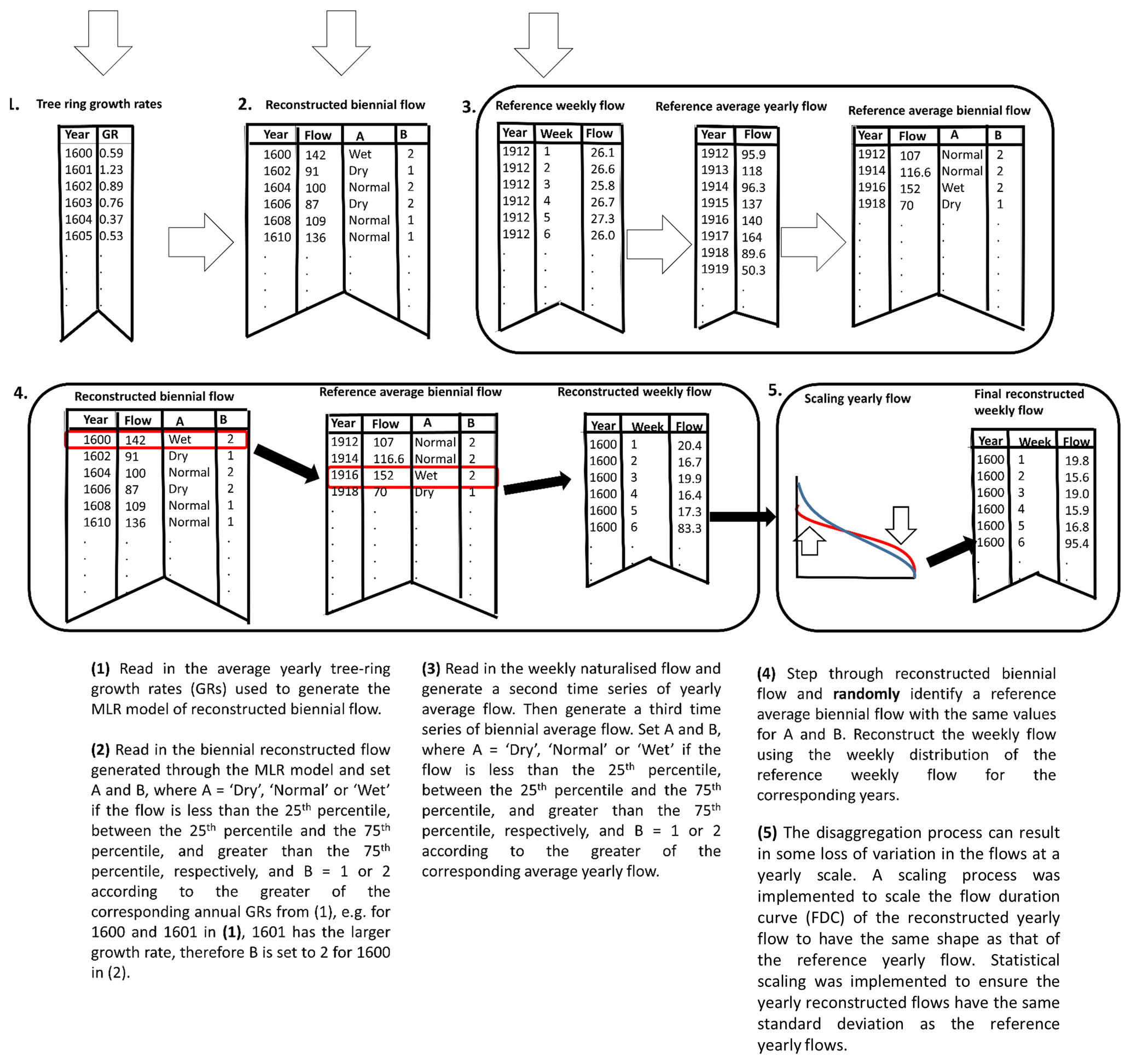
Figure 2Conceptual representation of the process for disaggregating 2-year (biennial) tree-ring reconstructed streamflow to weekly reconstructed streamflow.
As expected, the biennial reconstructed time series demonstrate smaller variability compared with the biennial flows in the reference period when MLR models are used for reconstruction, as the MLR models fitted by the least-squares method always produce smaller variance compared with the variance of observations. Therefore, the resulting annual and weekly time series also have less variability compared with their counterparts in the reference period. To rectify this problem, the reconstructed flows generated by stage (4) in Fig. 2 over the reference period (1912–2001) were compared to the reference flow at a yearly scale in the form of flow duration curves (FDCs). Typically, loss of variance in the reconstructed flows will manifest as fewer extreme high and low flows. A scaling equation was implemented to scale the FDC of the reconstructed flow to have the same shape as that of the reference flow:
where q′ is the scaled yearly reconstructed flow (m3 s−1), q is the yearly reconstructed flow (m3 s−1), P is the duration (%) and A, B and C are parameters that are calibrated by fitting the scaled yearly flow reconstructions for the reference period (1912–2001) to the yearly reference flow FDC.
In addition, the scaled yearly reconstructed flows were rescaled according to the mean and standard deviation of the yearly reference flows:
where and are the standard deviation and mean of the scaled yearly reconstructed flow for the reference period (1912–2001), respectively, Qstdev and Qmean are the standard deviation and mean of the yearly reference flow, respectively, and q′′ is the final (rescaled) yearly reconstructed flow for the entire reconstruction period (1600–2001).
This update of the yearly reconstructed flows was used to scale the weekly flow reconstructions, which were in turn scaled to have the same biennial average as the original biennial flow reconstructions.
2.3.3 Comparisons of autocorrelation between weekly flow reconstructions and reference flow
Weekly reference flows and weekly reconstructed flows were averaged to yearly over the reference period (1912–2001), and autocorrelation was calculated for different yearly time lags from 1 to 10 years. This was performed to confirm that the important statistical property of autocorrelation in the reference flows was carried over into the reconstructed flows.
3.1 Reconstruction of biennial flows based on tree-ring chronologies
MLR models with the best R2 values for each sub-basin were chosen to reconstruct biennial flows based on tree-ring chronologies (Table 1). A total of 4, 9, 6 and 10 MLR models were chosen for the North Saskatchewan, Oldman, Red Deer and Bow sub-basins, respectively, with R2 values ranging from 0.50 and 0.56, 0.44 and 0.51, 0.45 and 0.55, and 0.49 and 0.56, respectively. Figure 3 shows the time series of reconstructed 2-year (biennial) flows for all the MLR models shown in Table 1 for the four sub-basins, along with the reference flow over the calibration period.
Table 1Regression equations and R2 values obtained in 2-year (biennial) flow reconstructions using tree-ring chronologies for the Saskatchewan River basin. Tree-ring chronology site code definitions can be found in Sauchyn et al. (2011).
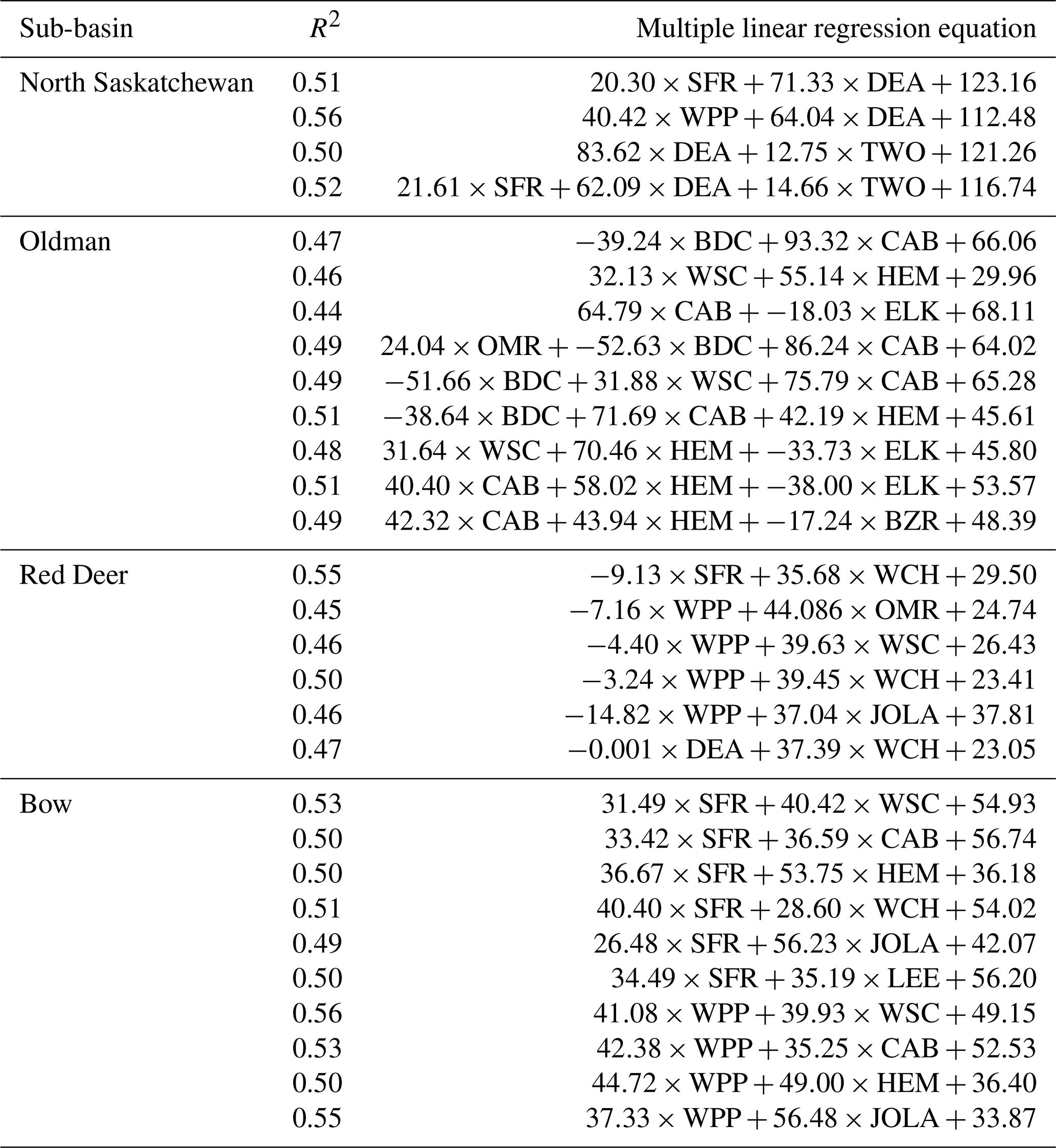
Figure 3 shows a relatively narrow distribution of reconstructed flows for the North Saskatchewan and Oldman sub-basins relative to those of the Red Deer and Bow River sub-basins, indicating a higher degree of uncertainty in the reconstructed flow for the latter pair of sub-basins. This could be related to the fact that the Red Deer and Bow River sub-basins contained few or none of the 16 tree-ring chronologies used in the biennial flow reconstructions.
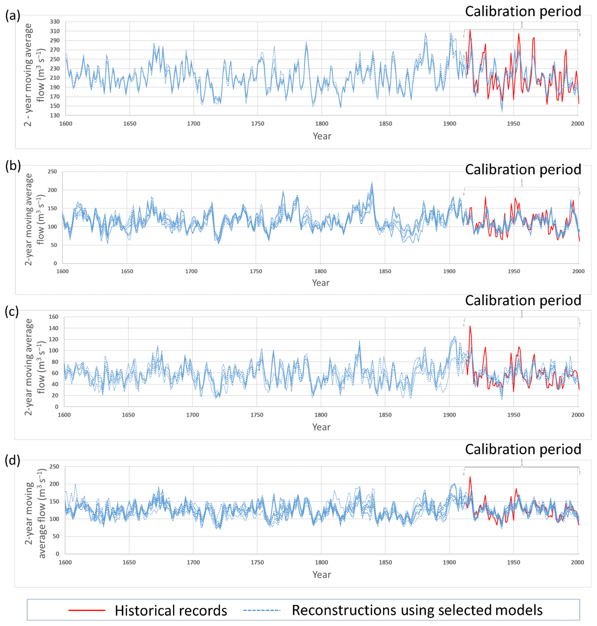
Figure 3Time series of reconstructed 2-year moving average (biennial) flows in the (a) North Saskatchewan, (b) Oldman, (c) Red Deer and (d) Bow rivers. The shown reconstructed flows for the calibration period are the results of cross-validation.
3.2 Disaggregation of 2-year (biennial) reconstructed flows to weekly flows
Figure 4 shows an example of how the scaling equation was derived for step (5) in Fig. 2 of the disaggregation process. This example is for Bow River for one of the MLR models and shows the FDCs of the yearly reconstructed flow up to step (4) and the yearly reference flow. The differences in the shapes of the FDCs illustrate some loss of variation in the reconstructed flows, with fewer extreme (high and low) flows. The values of A, B and C in Eq. (1) were changed to obtain a scaling of the reconstructed flow FDC to take a similar shape to that of the reference flow.
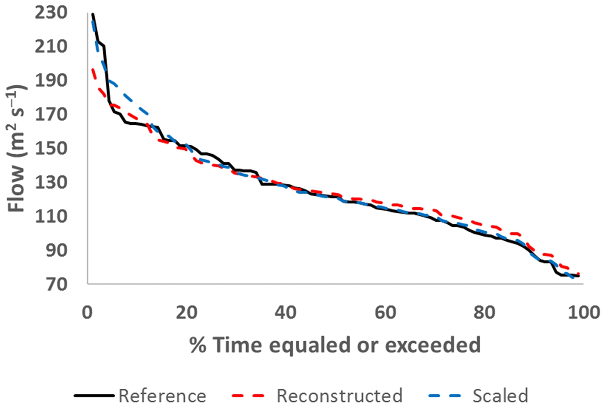
Figure 4An example of a comparison between a yearly flow reconstruction and yearly reference naturalized flow for the reference period (1912–2001) for Bow River using a flow duration curve (FDC). A scaling method was used to scale the yearly flow reconstruction FDC so that it would have the same shape as the FDC of the yearly reference flow.
For the present study, an ensemble of 30 weekly flow reconstructions for a single biennial flow reconstruction for each sub-basin was generated to illustrate the method. Figure 5 shows the ensemble time series of the weekly flow reconstructions in relation to the reference weekly naturalized flow for a short window of the reference period for the Oldman River. It is evident that the reconstructed flows have the correct timing and similar range of flows to the reference flow and also respond to periods of increased and decreased flow. However, further analysis was required to determine if the reconstructed flows have similar statistical properties to the reference flows.

Figure 5A time series comparison of an ensemble of 30 weekly flow reconstructions (dotted blue) and weekly naturalized flow (solid black) for the Oldman River basin.
Figure 6 shows the cumulative frequency distributions (CFDs) for the reconstructed flows in relation to the reference flows for a yearly time step, for both the reference period (1912–2001) and the full reconstruction period (1600–2001). The minimum and maximum bounds of the CFDs of the 30 reconstructed flows for the reference and full period are represented by the dotted red and dotted blue lines, respectively, whereas the CFD for the reference flow is indicated by the solid black line.
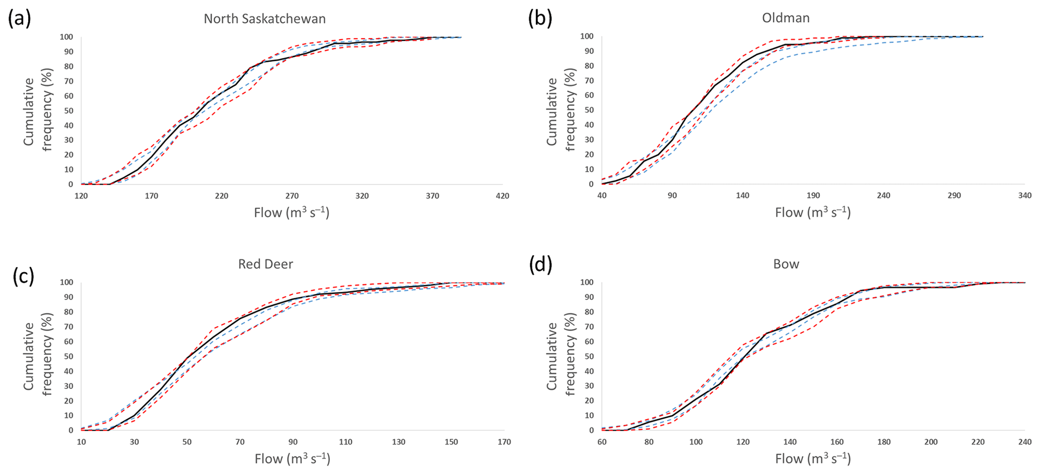
Figure 6Cumulative frequency distributions (CFDs) between reconstructed flow and reference naturalized flow at a yearly time step. The minimum and maximum bounds of the CFDs of the 30 reconstructed flows for the reference and full period are represented by the dotted red and dotted blue lines, respectively, whereas the CFD for the reference flow is indicated by the solid black line: (a) North Saskatchewan River, (b) Oldman River, (c) Red Deer River (d) Bow River.
It is evident from Fig. 6 that for each sub-basin, the bounds of the CFDs for reconstructed flows for the reference period encompass the CFD of the reference flow. The bounds of the CFDs for reconstructed flows for the full period show some shifts in some cases compared to the reference flow. For example, the reconstructed flows for the Oldman River for the full period appear to be slightly higher than those of the reference period (Fig. 6b), whereas the reconstructed flows for the North Saskatchewan River over the full period may have a smaller proportion of high flows compared to the reference period (Fig. 6a). It is important to emphasize that this example considers only one reconstruction model for each sub-basin, and Fig. 3 shows a fairly high variability between reconstructions for some sub-basins; therefore, the final set of flow reconstructions will contain considerably higher variability.
Figure 7 shows a comparison of autocorrelation for reconstructed and reference flows for the reference period 1912–2001 at a yearly time step for each sub-basin, where the dotted red lines indicate the maximum and minimum of the autocorrelation values of the 30 flow reconstructions and the solid black line is the autocorrelation of the reference flow. It is evident in Fig. 7 for all sub-basins for both the reconstructed and reference flows, i.e. for each sub-basin, the autocorrelations of the reconstructed flows are generally comparable with that of the reference flow.

Figure 7A comparison of autocorrelation between the 30 reconstructed flows and reference naturalized flow at a yearly time step over the reference period (1912–2001), where the dotted red lines indicate the maximum and minimum bounds of the autocorrelation values of the 30 reconstructed flows and the solid black line indicates the autocorrelation of the reference flow: (a) North Saskatchewan River, (b) Oldman River, (c) Red Deer River, and (d) Bow River.
Biennial reconstructions achieved for the four sub-basins in the present study were generally broadly similar to 5-year reconstructions obtained for the same sub-basins by Razavi et al. (2016) using the same set of tree-ring chronologies. The major differences between the results of the present study and those of Razavi et al. (2016) are higher variation in the reconstructed flows and greater divergence between the reconstructed flows for individual sub-basins for the present study (Fig. 3). This can be related to the fact that Razavi et al. (2016) found a stronger relationship between flow and tree-ring chronologies on a 5-year time step, whereas the present study used a 2-year time step. The R2 values achieved for 5-year flow reconstructions by Razavi et al. (2016) were higher in addition, ranging from 0.54 to 0.72, whereas R2 values achieved in the present study ranged from 0.44 to 0.56. The present study established the relationship between flow and tree-ring chronologies on a 2-year time step as a compromise to more easily facilitate the disaggregation of flows while still achieving a relatively strong relationship between flows and tree-ring chronologies and overcoming the discrepancies in persistence between flow and tree-ring chronologies without resorting to pre-whitening techniques.
While the MLR R2 values obtained in the current study are within the range of those of previous studies describing the relationship between tree-ring chronologies and river flow, the present study did not focus merely on improving the regression fits. Instead, it introduced a method that first constructs these relationships between tree-ring chronologies and naturalized flow in a way that preserves persistence properties and variability of hydrological time series and second introduces a novel method of disaggregating biennial reconstructed flow to weekly flows. The uncertainty, firstly in the relationships between tree-ring chronologies and naturalized flow and secondly within the disaggregation technique, is addressed through an ensemble approach, by producing a range of viable MLR models for individual catchments and multiple plausible flow time series within the disaggregation. The selection of the number of regressors was based on a former study with the same data (Razavi et al., 2016), where the Akaike Information Criterion was used to limit the risk of over-parametrization and overfitting.
The tree growth and water availability, as represented by tree-ring width and streamflows here, respectively, are always positivity correlated in moisture-limited settings (although this is not necessarily true in energy-limited settings). This means that a regression coefficient in a single linear regression should always be positive. However, as evident from the negative coefficients of the MLR models shown in Table 1, in multiple linear regression, the signs of some of the coefficients might become negative because of collinearity, which relates to the dependence of the tree-ring chronologies. The application of principal component analysis (PCA) to the regressors before doing regression is a way of circumventing collinearity and avoiding negative coefficients in the models. Although not reported here, PCA was applied to the tree-ring chronologies and results of MLR with and without PCA were compared, with no noticeable difference found.
We note that tree rings provide no meaningful information on sub-annual variability. Therefore, the process of disaggregating 2-year (biennial) tree-ring reconstructed streamflow to weekly reconstructed streamflow is merely statistical, based on the information on the seasonality in the reference record. As such, a caveat of this approach is the absence of information on any possible change in seasonality due to climate change effects. Although, from a water resources modelling perspective, the longer-term inter-year variability is arguably more important to represent than intra-year variability; for example, it would be persistent long-term droughts that challenge the robustness of water resource systems. The discussion below shows that statistical properties of the reference flows are preserved in the reconstructed flows. This is important as the outcomes of modelling studies that would use these flows will depend largely on the presence of these statistical properties.
The approach of using the weekly distribution of the reference flow within the disaggregation of biennial reconstructed flows (see Fig. 2, step 4), along with the scaling of the yearly reconstructed flow (see Fig. 2, step 5), appears to resolve the issue of discrepancies in variation and persistence between the reconstructed and reference flow. Figure 5 shows that the weekly reconstructed flow displays the same timing and range of flow in comparison to the reference flow and also similar timing for dry and wet periods. Figures 5 and 6 show that the disaggregation approach used was successful in replicating the variance in the reference flow within the reconstructed flow. The persistence between flows for both the reference and reconstructed flows were similar, and both showed a generally decreasing trend with increasing time lag (Fig. 7).
Razavi et al. (2016) showed that tree-ring chronologies and flows at the annual timescale may possess inconsistent persistence properties. This inconsistency leads to dissimilar patterns of change and variability in the two types of time series across other timescales, which might invalidate any resulting flow reconstructions. To investigate this, Fig. 8 shows the variance of the reconstructed and reference flows at different timescales on a log–log scale for the four sub-basins. The variance values at different timescales were calculated through averaging; for example, a flow period of 100 years would yield 50 and 10 values when the average of every 2 and 10 years is calculated, respectively. The graph represents variance of the different time series over different timescales. The slopes of the different time series can be benchmarked against a random process (the dotted red line in the plot), which contains no persistence at any timescale. The differences in slopes between the reconstructed and reference flows shown in Fig. 8 compared to that of the random process can be attributed to persistence at the range of timescales represented. Razavi et al. (2016), using a similar plot, showed that tree-ring growth rates have considerably different persistence at shorter timescales compared to flow, and this persistence could be expected to be transferred to flow reconstructed from tree-ring chronologies using relationships established at shorter timescales. The slope associated with reference flow would however be closer to that of the random process at a shorter timescale. Figure 8 demonstrates that the flow reconstruction and disaggregation method used in the present study appears to overcome the problem of transferal of higher persistence in tree-ring chronologies to the reconstructed flow at shorter timescales. The slopes of both the reference and reconstructed flows appear to be similar. This indicates that the reconstructed flows have similar persistence to the reference flows across the entire reference flow period of 90 years. Variance versus timescale plots provide a method of studying the “Hurst Phenomenon” for long-term persistence in hydrologic time series (Hurst, 1951).
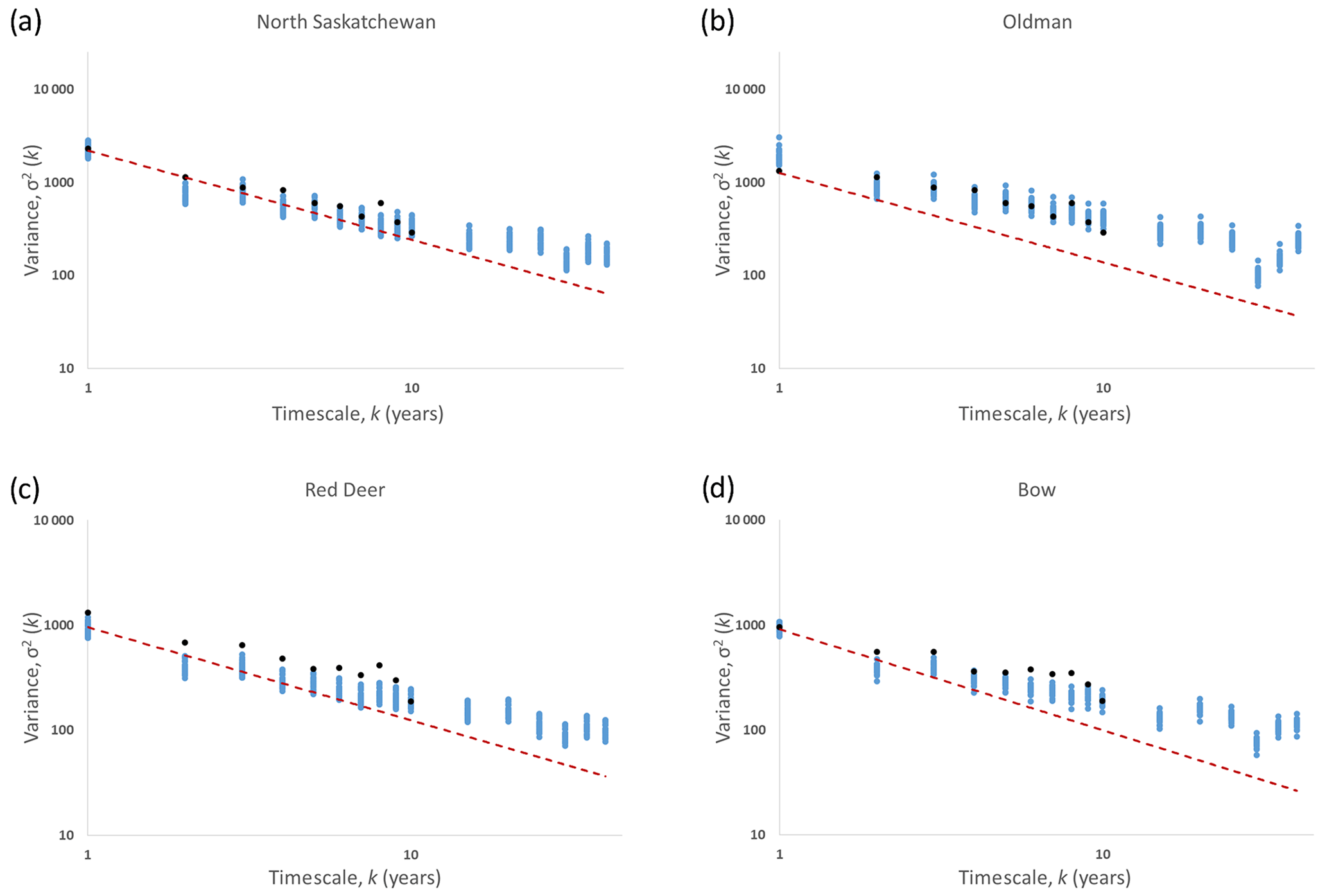
Figure 8Variance versus timescale plot for reference and reconstructed flows in the (a) North Saskatchewan, (b) Oldman, (c) Red Deer and (d) Bow rivers. Black and blue time series represent reference and reconstructed flows, respectively, whereas the red line represents a random process with no long-term persistence.
The present study reconstructed biennial flows based on MLR models of the relationship between tree-ring chronologies and observed flow in the reference period, and an argument can be made that changes in recent physical processes due to climate change could have distorted this relationship. Indeed, with increasing snowmelt under a warming climate, the underlying statistical properties of flow in a water-tower-driven catchment such as the SaskRB may indeed change considerably compared to the pre-reference period. However, since the reference period used ended in 2000, which is now almost 20 years ago, we assume that the more recent climate change trends were absent or at least much weaker prior to the turn of the century.
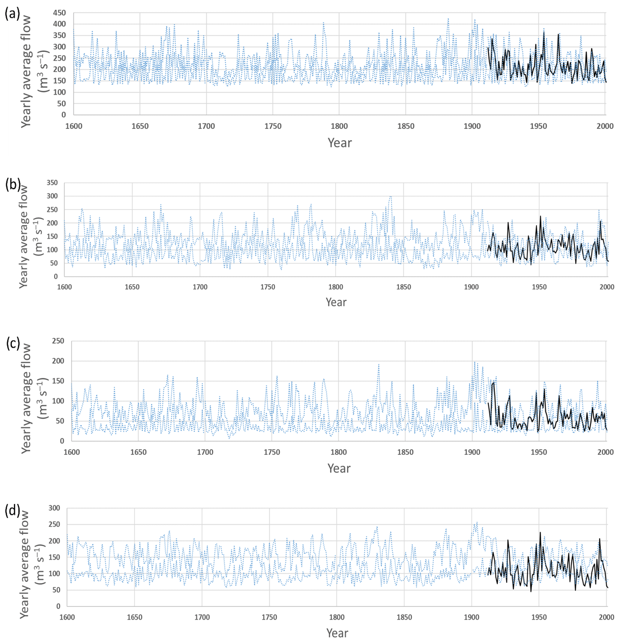
Figure 9Time series of reconstructed yearly average flows in (a) North Saskatchewan, (b) Oldman, (c) Red Deer and (d) Bow rivers, showing the 5th and 95th percentile range of the ensemble of 500 time series flows as a representation of uncertainty for 1600–2001 (dotted blue lines) as well as the observed reference flow (solid black line).
In the present study, the reconstructions of biennial flow for the North Saskatchewan and Oldman River sub-basins showed lower divergence compared to those for the Red Deer and Bow River sub-basins (Fig. 3). This indicates a higher degree of uncertainty in the flow reconstructions for the Red Deer and Bow River sub-basins and is due to the fact that few or none of the 16 tree-ring chronologies used occurred in these sub-basins. There are many additional uncertainties in the statistical relationships constructed between flow and tree-ring chronologies (Razavi et al., 2016). These uncertainties are amplified by the further disaggregation of biennial flow reconstructions to weekly flows. An approach to represent this uncertainty is to generate a large reconstructed flow ensemble. Uncertainty within the statistical relationship between flow and tree-ring chronologies can be represented by using multiple acceptable MLR models. For each biennial reconstructed flow generated by a single MLR model, the uncertainty in the disaggregation process can be represented by generating a large number of weekly reconstructed flows. In the present study, the number of weekly reconstructed flows generated for each acceptable MLR model was chosen to obtain an ensemble of 500 weekly flow time series for each sub-basin. To demonstrate the full range of uncertainty of the reconstructed flows, Fig. 9 shows the yearly average flow range (5th and 95th percentiles) of the 500 time series of weekly reconstructed flows for each sub-basin. It is evident that the higher uncertainty between reconstructed biennial flows, as represented in Fig. 3, results in higher uncertainty in the weekly flow reconstructions, as represented in Fig. 9. For example, there are relatively few differences between the biennial flow reconstructions for the North Saskatchewan River (Fig. 3a), and this results in relatively small uncertainty in the weekly flow reconstructions (Fig. 9a), whereas the large uncertainties in the biennial flow reconstructions for the Red Deer (Fig. 3c) translate into larger uncertainty in the corresponding weekly flow reconstructions (Fig. 9c). In general, Fig. 9 shows that there is a large uncertainty range in the weekly flow reconstructions. Reducing the total uncertainty in the weekly flow reconstructions therefore requires establishing stronger statistical relationships between the reference biennial flow and biennial tree-ring chronologies for each sub-basin. If new tree-ring chronology data falling within the Red Deer River and Bow River catchments become available, future studies could attempt to establish stronger statistical relationships with the reference flow for these two sub-basins.
The data generated in this study are available from https://doi.org/10.20383/101.0139 (Slaughter and Razavi, 2019).
The tree-ring data used in this paper are archived in the International Tree-ring Data Bank (ITRDB), available online at http://www.ncdc.noaa.gov/data-access/paleoclimatology-data/datasets/tree-ring (NOAA, 2020).
This study presented a novel method for generating weekly flows for a period preceding the period of record, based on tree-ring data, while maintaining the statistical properties of the reference (measured) flows, including variability and persistence across all timescales. The method featured two novel components; unlike the conventional approach that mainly bases the analysis on annual (or sub-annual) flow chronology correlations, the method (i) first reconstructs flows on a biennial (2-year) scale, which demonstrates higher correlation with chronologies (tree growth), thereby resulting in a higher explanatory power, and (ii) then disaggregates the biennial flows into annual and weekly scales based on information contained in the annual chronologies and weekly flow data in the reference period. The weekly reconstructed flows for the Saskatchewan River basin, a large river basin in Western Canada, which is of great social and economic importance, facilitates the investigation of multiple flow futures, which could contribute to increasing the resilience of the basin to future climatic changes.
SR provided guidance for all aspects of the study and critically evaluated the methods and results as well as the manuscript. SR specified the statistical techniques used, a broad concept of the disaggregation technique and the methods used to validate the results. ARS conducted all analyses, wrote the code for the disaggregation technique and prepared the manuscript.
The authors declare that they have no conflict of interest.
This article is part of the special issue “Water, ecosystem, cryosphere, and climate data from the interior of Western Canada and other cold regions”. It is not associated with a conference.
The authors wish to acknowledge David Sauchyn and the Prairie Adaptation Research Collaborative (PARC) at the University of Regina for generating the tree-ring data used in this paper. The International Tree-ring Data Bank (ITRDB) is acknowledged for providing access to the tree-ring data used in this study.
This research has been supported by the Integrated Modelling Program for Canada (IMPC) and the Global Wate Futures (GWF).
This paper was edited by Chris DeBeer and reviewed by two anonymous referees.
Agafonov, L. I., Meko, D. M., and Panyushkina, I. P.: Reconstruction of Ob River, Russia, discharge from ring widths of floodplain trees, J. Hydrol., 543, 198–207, 2016.
Alberta Environment: Water Resources Management Model (WRMM), Government of Alberta, Edmonton, Alberta, 2002.
Axelson, J. N., Sauchyn, D. J., and Barichivich, J.: New reconstructions of streamflow variability in the South Saskatchewan River Basin from a network of tree ring chronologies, Alberta, Canada, Water Resour. Res., 45, W09422, https://doi.org/10.1029/2008WR007639, 2009.
Boucher, Ė., Ouarda, T. B. M. J., Bėgin, Y., and Nicault, A.: Spring flood reconstruction from continuous and discrete tree ring series, Water Resour. Res., 47, W07516, https://doi.org/10.1029/2010WR010131, 2011.
Brigode, P., Brissette, F., Nicault, A., Perreault, L., Kuentz, A., Mathevet, T., and Gailhard, J.: Streamflow variability over the 1881–2011 period in northern Québec: comparison of hydrological reconstructions based on tree rings and geopotential height field reanalysis, Clim. Past, 12, 1785–1804, https://doi.org/10.5194/cp-12-1785-2016, 2016.
Case, R. A. and MacDonald, G. M.: Tree ring reconstructions of streamflow for three Canadian prairie rivers, J. Am. Water Resour. As., 39, 703–716, 2003.
Cohn, T. A. and Lins, H. F.: Nature's style: Naturally trendy, Geophys. Res. Lett., 32, L23402, https://doi.org/10.1029/2005GL024476, 2005.
Cook, E. R., Woodhouse, C. A., Eakin, C. M., Meko, D. M., and Stahle, D. W.: Long-term aridity changes in the Western United States, Science, 306, 1015–1018, 2004.
Elshorbagy, A., Wagener, T., Razavi, S., and Sauchyn, D.: Correlation and causation in tree-ring-based reconstruction of paleohydrology in cold semiarid regions, Water Resour. Res., 52, 7053–7069, 2016.
Ferrero, M. E., Villalba, R., De Membiela, M. D., Hidalgo, L. F., and Luckman, B. H.: Tree-ring based reconstruction of Río Bermejo streamflow in subtropical South America, J. Hydrol., 525, 572–584, 2015.
Gangopadhyay, S., Harding, B. L., Rajagopalan, B., Lukas, J. J., and Fulp, T. J.: A nonparametric approach for paleohydrologic reconstruction of annual streamflow ensembles, Water Resour. Res., 45, W06417, https://doi.org/10.1029/2008WR007201, 2009.
Hurst, H. E.: Long-term storage capacity of reservoirs, T. Am. Soc. Civ. Eng., 116, 770–808, 1951.
Lara, A., Bahamondez, A., González-Reyes, A., Muñoz, A. A, Cuq, E., and Ruiz-Gómez, C.: Reconstructing streamflow variation of the Baker River from tree-rings in Northern Patagonia since 1765, J. Hydrol., 529, 511–523, 2015.
Martz, L., Armstrong, R., and Pietroniro, E.: Climate Change and Water: SSRB Final Technical Report, GIServices, University of Saskatchewan: Saskatoon, Canada, 2007.
Maxwell, R. S., Hessl, A. E., Cook, E. R., and Pederson, N.: A multispecies tree ring reconstruction of Potomac River streamflow (950–2001), Water Resour. Res., 47, W05512, https://doi.org/10.1029/2010WR010019, 2011.
Milly, P. C. D., Betancourt, J., Falkenmark, M., Hirsch, R. M., Kundzewicz, Z. W., Lettenmaier, D. P., and Stouffer, R. J.: Stationarity is dead: whither water management?, Science, 319, 573–574, 2008.
Mokria, M., Gebrekirstos, A., Abiyu, A., and Bräuning, A.: Upper Nile River flow reconstructed to A.D. 1784 from tree-rings for a long-term perspective on hydrologic-extremes and effective water resource management, Quaternary Sci. Rev., 199, 126–143, 2018.
NOAA: Tree-ring Data, available online at: http://www.ncdc.noaa.gov/data-access/paleoclimatology-data/datasets/tree-ring, last access: February 2020.
Pomeroy, J., De Boer, D., and Martz, L.: Hydrology and water resources of Saskatchewan, Center for Hydrology, Report no. 1, Saskatoon, Canada, 2005.
Razavi, S. and Vogel, R.: Prewhitening of hydroclimatic time series? Implications for inferred change and variability across time scales, J. Hydrol., 557, 109–115, 2018.
Razavi, S., Elshorbagy, A., Wheater, H., and Sauchyn, D.: Toward understanding nonstationarity in climate and hydrology through tree ring proxy records, Water Resour. Res., 51, 1813–1830, https://doi.org/10.1002/2014WR015696, 2015.
Razavi, S., Elshorbagy, A., Wheater, H., and Sauchyn, D.: Time scale effect and uncertainty in reconstruction of paleo-hydrology, Hydrol. Process., 30, 1985–1999, 2016.
Sauchyn, D. and Ilich, N.: Nine hundren years of weekly streamflows: stochastic downscaling of ensemble tree-ring reconstructions, Water Resour. Res., 53, 9266–9283, https://doi.org/10.1002/2017WR021585, 2017.
Sauchyn, D., Vanstone, J., and Perez-Valdivia, C.: Modes and forcing of hydroclimatic variability in the Upper North Saskatchewan River Basin since 1063, Can. Water Resour. J., 36, 205–218, 2011.
Slaughter, A. and Razavi, S.: An ensemble of 500 time series of weekly flows from 1600–2001 for the four sub-basins of the Saskatchewan River Basin generated through disaggregating tree-ring reconstructed flow [Dataset], Federated Research Data Repository, https://doi.org/10.20383/101.0139, 2019.
Urrutia, R. B., Lara, A., Villalba, R., Christie, D. A., Le Quesne, C., and Cuq, A.: Multicentury tree ring reconstruction of annual streamflow for the Maule River watershed in south central Chile, Water Resour. Res., 47, W06527, https://doi.org/10.1029/2010WR009562, 2011.
Woodborne, S., Hall, G., Robertson, I., Patrut, A., Rouault, M., Loader, N. J., and Hofmeyer, M.: A 1000-Year Carbon Isotope Rainfall Proxy Record from South African Baobab Trees (Adansonia digitata L.), PLOS ONE, 10, e0124202, https://doi.org/10.1371/journal.pone.0124202, 2015.
Woodhouse, C. A. and Lukas, J. J.: Drought, tree rings and water resource management in Colorado, Can. Water Resour. J., 31, 297–310, 2006.
Woodhouse, C. A., Gray, S. T., and Meko, D. M.: Updated streamflow reconstructions for the Upper Colorado River Basin, Water Resour. Res., 42, W05415, https://doi.org/10.1029/2005WR004455, 2006.