the Creative Commons Attribution 4.0 License.
the Creative Commons Attribution 4.0 License.
 | 02 Sep 2020
Earth transformed: detailed mapping of global human modification from 1990 to 2017
Christina Kennedy
Bin Chen
James Oakleaf
Sharon Baruch-Mordo
Joe Kiesecker
Data on the extent, patterns, and trends of human land use are critically important to support global and national priorities for conservation and sustainable development. To inform these issues, we created a series of detailed global datasets for 1990, 2000, 2010, and 2015 to evaluate temporal and spatial trends of land use modification of terrestrial lands (excluding Antarctica). We found that the expansion of and increase in human modification between 1990 and 2015 resulted in 1.6 M km2 of natural land lost. The percent change between 1990 and 2015 was 15.2 % or 0.6 % annually – about 178 km2 daily or over 12 ha min−1. Worrisomely, we found that the global rate of loss has increased over the past 25 years. The greatest loss of natural lands from 1990 to 2015 occurred in Oceania, Asia, and Europe, and the biomes with the greatest loss were mangroves, tropical and subtropical moist broadleaf forests, and tropical and subtropical dry broadleaf forests. We also created a contemporary (∼2017) estimate of human modification that included additional stressors and found that globally 14.6 % or 18.5 M km2 (±0.0013) of lands have been modified – an area greater than Russia. Our novel datasets are detailed (0.09 km2 resolution), temporal (1990–2015), recent (∼2017), comprehensive (11 change stressors, 14 current), robust (using an established framework and incorporating classification errors and parameter uncertainty), and strongly validated. We believe these datasets support an improved understanding of the profound transformation wrought by human activities and provide foundational data on the amount, patterns, and rates of landscape change to inform planning and decision-making for environmental mitigation, protection, and restoration.
The datasets generated from this work are available at https://doi.org/10.5281/zenodo.3963013 (Theobald et al., 2020).
Please read the corrigendum first before continuing.
-
Notice on corrigendum
The requested paper has a corresponding corrigendum published. Please read the corrigendum first before downloading the article.
-
Article
(5999 KB)
-
The requested paper has a corresponding corrigendum published. Please read the corrigendum first before downloading the article.
- Article
(5999 KB) - Full-text XML
- Corrigendum
- BibTeX
- EndNote


Humans have transformed the Earth in profound ways (Marsh, 1885; Jordan et al., 1990; Vitousek et al., 1997; Hurtt et al., 2006), contributing to global climate change (IPCC, 2019), causing global habitat loss and fragmentation, and contributing to declines in biodiversity and critical ecosystem services (IPBES, 2019). Addressing the consequences of rapid habitat loss and land use change is essential for the implementation of various international initiatives, including the Convention on Biological Diversity 2020 Aichi Biodiversity Targets, the United Nations 2030 Sustainable Development Goals (especially Goal 15; Secretariat of the Convention on Biological Diversity, 2010), the Bonn Challenge (Verdone and Seidl, 2017), and the Global Deal for Nature (Dinerstein et al., 2019). Foundational to addressing these goals is a firm understanding of the rates, trends, and extent of these land use changes. Efforts to date have focused on historical patterns (Klein Goldewijk et al., 2007, 2017; Ramankutty et al., 2008; Ellis, 2018) or have been limited due to the unavailability of contemporary, temporally comparable, and high-resolution (<1 km2) data (Venter et al., 2016; Geldmann et al., 2019a; Kennedy et al., 2019b).
Here we describe a new dataset that maps the degree of human modification of terrestrial ecosystems globally, for recent changes from 1990 to 2015 and for contemporary (circa 2017) conditions. We mapped human activities that directly or indirectly alter natural systems, which we call anthropogenic drivers of ecological stress or “stressors” (following Salafsky et al., 2008; Theobald, 2013). Similarly to other efforts (Sanderson et al., 2002; Theobald, 2010, 2013; Geldmann et al., 2014; Venter et al., 2016; Kennedy et al., 2019b), we augmented remotely sensed data with traditionally mapped cartographic features. This is because remotely sensed imagery has limitations for this application – especially prior to ∼2010 – because it can require human interpretation to classify adequately and can miss development features that are obstructed by vegetation canopy or are small or narrow features (e.g., towers, wind turbines, power lines).
We mapped the degree of human modification based on an established approach that has been applied nationally, internationally, and globally (Theobald, 2010, 2013; González-Abraham et al., 2015; Kennedy et al., 2019b). It uses an existing classification system (Salafsky et al., 2008) to (a) ensure parsimony, (b) distinguish two spatial components (area of use and intensity of use), (c) use a physically based measure that is needed to estimate change (Gardner and Urban, 2007), (d) incorporate spatial and classification uncertainty, and (e) combine multiple stressors into an overall measure that assumes additive relationships among stressors and addresses the correlation among variables (Theobald, 2010). The resulting quantitative estimate of human modification has values ranging from 0 to 1 that support robust landscape assessments (Schultz, 2001; Hajkowicz and Collins, 2007).
To understand temporal landscape change, we calculated the degree of human modification – denoted by H – for the years 1990, 2000, 2010, and 2015 using methods and datasets that minimize noise and bias. Second, we included additional stressors not incorporated previously, including disturbance of natural processes due to reservoirs, effects from air pollution, and human intrusion (Theobald, 2008). Third, we calculated human stressors using data that are of a resolution up to 2 orders of magnitude finer (0.09 vs. 1–86 km2) than past efforts (Ellis and Ramankutty, 2008; Geldmann et al., 2014, 2019a; Haddad et al., 2015; Venter et al., 2016; Kennedy et al., 2019b). This higher resolution reduces the loss of information of the spatial pattern within a pixel; better identifies rare features; facilitates the application of these data for species and ecological processes that often occur at a fine scale; and improves the utility and relevance of these products for policy makers, decision makers, and land use managers.
Calculating H as a real value across the full gradient of landscape change is valuable because it can be applied rigorously to a variety of questions (Theobald, 2010, 2013), including discerning the heterogeneity of human uses that are often lumped within broad classes like “urban”, capturing the extent and pattern of the agricultural lands typically occurring beyond urban centers and protected areas, and delineating areas of low modification, all of which are useful for conservation prioritization and planning efforts (Kennedy et al., 2019b, c). Here, we describe the technical methods and briefly report on results on the temporal trends and current spatial patterns of human modification across all terrestrial lands, continents, biomes, and ecoregions. Because conservation organizations often use these types of data to focus their activities on specific regions (e.g., Jantke et al., 2019), we provide rankings by biome and ecoregion (Dinerstein et al., 2017) and briefly compare our results to other available studies.
2.1 Overview
We calculated the degree of human modification using the Direct Threats Classification v2 (Salafsky et al., 2008; http://cmp-openstandards.org, last access: 28 December 2019), which defines a stressor as the proximate human activities or processes that have caused, are causing, or may cause impacts on biodiversity and ecosystems. Table 1 lists the specific stressors and data sources we included in our maps: urban and built-up, crop and pasture lands, livestock grazing, oil and gas production, mining and quarrying, power generation (renewable and nonrenewable), roads, railways, power lines and towers, logging and wood harvesting, human intrusion, reservoirs, and air pollution.
Table 1Overview of stressors, datasets, spatial resolution, and years data were available and used in the maps of human modification. Stressor classification levels in parentheses correspond to those within the Direct Threats Classification v2 (Salafsky et al., 2008). Acronyms of source data are in bold in the “Source” column for reference throughout the paper. For each stressor, the years 1990–2015 are used for change analysis, and ∼2017 is a compilation of all stressors that represents “current” conditions with the median year of 2017.
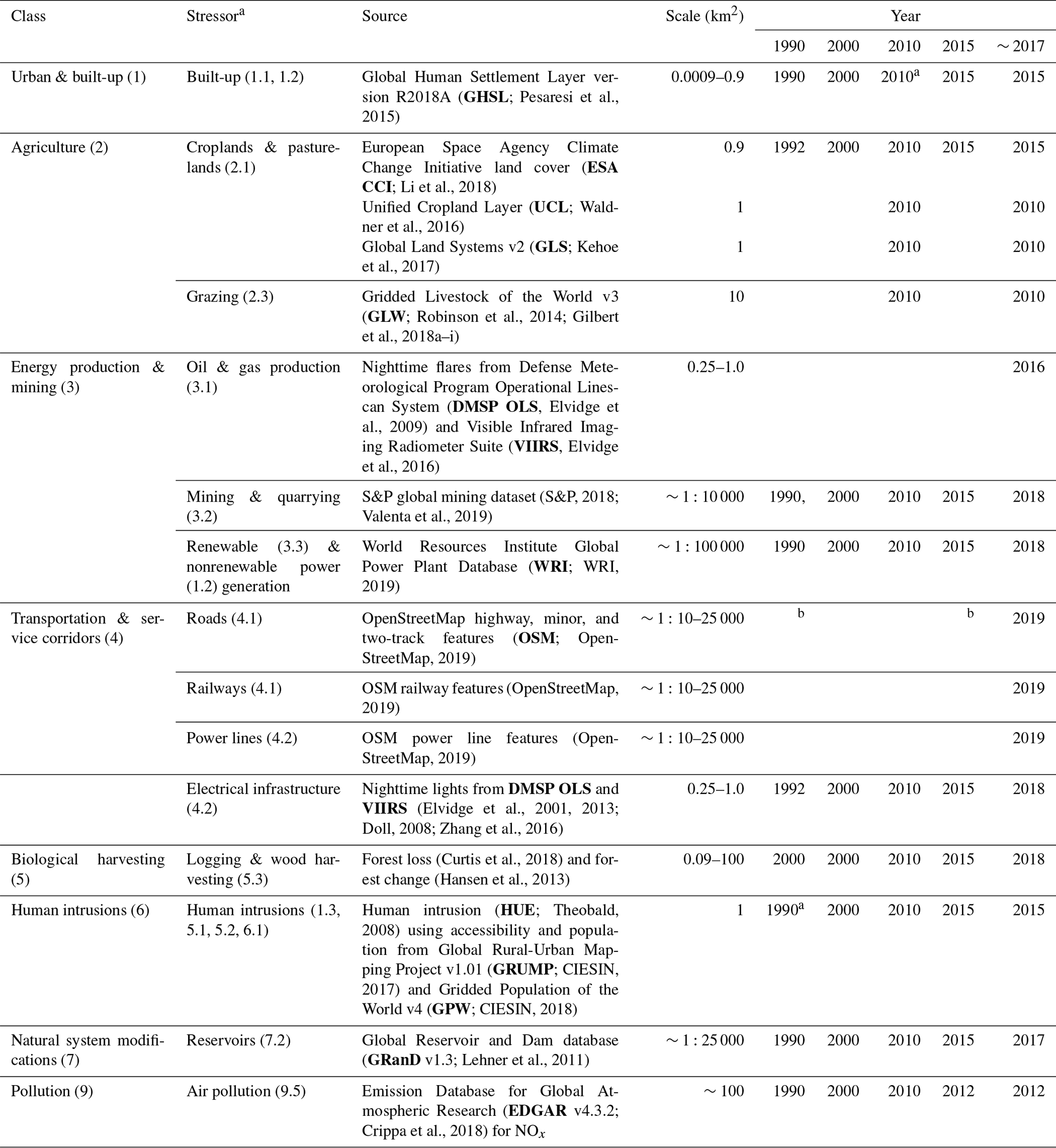
a Based on interpolation. b Used major roads (i.e., highways) for 2019.
To estimate temporal change in H from 1990 to 2015, we followed established criteria (Geldmann et al., 2014) and included 11 stressors for which we could obtain global data with a fine-grained resolution (≤1 km2) and that provided consistent and comparable repeated measurements, especially in regards to the data source, methods used, and appropriate time frame (Table 1). We included current major roads and railways as a static layer in the temporal maps because in most cases some form of road existed prior to our baseline year of 1990 (except for the relatively rare, though important, new highways constructed).
To estimate the current amount of H circa 2017 (median = 2017, min = 2012, max = 2019), we included three additional stressors, comprising grazing, oil and gas wells, and power lines. We note that we did not map stressors for invasive species or pathogens and genes, geologic events, or climate change. This was because suitable temporal global data were not available to capture stressors due to invasive species or pathogens and genes, the majority of geological events is not directly caused by humans, and climate change is better modeled as a separate process distinct from the effects of direct human activities and there is a plethora of research on this topic (Geldmann et al., 2014; Titeux et al., 2016).
Table 2Estimates of the intensity value for each stressor. “Best” estimates were determined from Brown and Vivas (2005)1, Theobald (2013)2, Kennedy et al. (2019b)3, or expert judgment4 and are bracketed by a minimum and maximum range, following the lowest–highest–best-estimate elicitation procedure to reduce bias (McBride et al., 2012). Results presented here use the best estimate, while minimum and maximum estimates are used to specify the range of possible randomized intensity values in the uncertainty analysis.
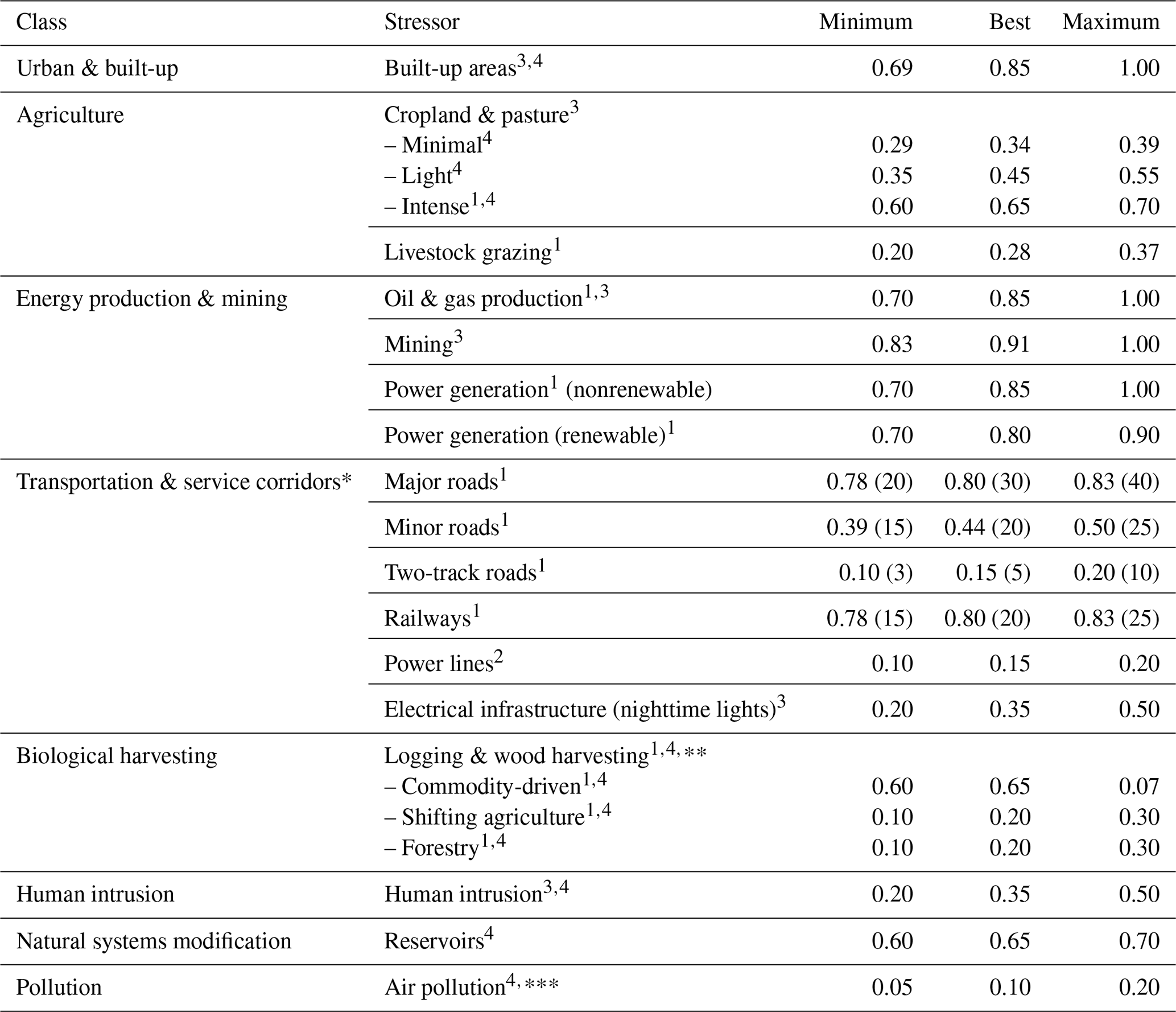
∗ Assumed width of roads and railways (meters) provided in parentheses. Use of
roads is incorporated into estimates of human intrusion.
Forest loss due to wildfire was not included because of the
challenges in understanding human causation and suppression, especially over a
global extent. Also, loss due to urbanization was not included in
this stressor because it is incorporated directly into the built-up stressor.
Minimum value is half of best; maximum is twice the best.
For each stressor s we quantified the degree of human modification as
where Fs is the proportion of a pixel occupied (i.e., the footprint) by stressor s, p(Cs) is the probability that a stressor occurs at a location to account for spatial and classification uncertainty, and Is is the intensity. Importantly, F and I have a direct physical interpretation (Gardner and Urban, 2007), are well bounded, and range from 0 to 1 and values are a “real” data type. Consequently, H provides the basis for unambiguous interpretation to assess landscape change (Hajkowicz and Collins, 2007; Riitters et al., 2009). Specific formulas used to map raw stressor data as indicator layers are provided below. Table 2 details our estimates of intensity values for each stressor (modified from Theobald, 2013; Kennedy et al., 2019b), which is used to differentiate land uses that have varying impacts on terrestrial systems (e.g., grazing is less intensive than mining). Our intensity values were informed by standardized measures of the amount of nonrenewable energy required to maintain human activities (Brown and Vivas, 2005) and found to generally correlate with species' responses to land use where examined (Kennedy et al., 2019b).
We generated datasets that represent temporal changes between 1990 and 2015 and for current (∼2017) conditions by combining stressor layers using the fuzzy algebraic sum (Bonham-Carter, 1994; Malczewski, 1999; Theobald, 2013), which is calculated as
where n is the number of stressors (s) included. Of critical importance, the fuzzy sum formula is an increasive function that calculates the cumulative effects of multiple stressors in a way that minimizes the bias associated with nonindependent stressors and assumes that multiple stressors accumulate (Theobald, 2010, 2013; Kennedy et al., 2019b). This differs substantially from simple additive calculations that are commonly used (Halpern et al., 2008; Halpern and Fujita, 2013; Venter et al., 2016) but assume that stressors are independent and results in a metric that is sensitive to the number of stressors included in the model (Malczewski, 1999).
We mapped human modification of all terrestrial lands (excluding Antarctica) and included lands inundated by reservoirs but excluded other rivers and lakes. An often overlooked but critical aspect to understanding human modification is how water is mapped, especially for the interface between land and coastlines, lakes, reservoirs, and large rivers. We mapped nonreservoir areas dominated by water (i.e., oceans, lakes, reservoirs, and rivers) by processing data on ocean from the European Space Agency's Climate Change Initiative program (ESA CCI; 0.15 km, circa 2000) and on surface waters using the Global Surface Water dataset (GSW; 30 m; Pekel et al., 2016). We identified inland water bodies (i.e., lakes, reservoirs, rivers, etc.) using ESA CCI nonocean pixels that were at least 1 km from the interior of the land–ocean interface. We identified interior water pixels using GSW with at least 75 % water occurrence from 1984 to 2019 and that were at least 0.0225 km2 in area (to remove small lakes, ponds, and narrow streams). As a result, inland water bodies and the ocean–land interface are more distinct, more consistent, and better aligned.
We summarized our estimates of human modification across all terrestrial lands, biomes, and ecoregions (defined by Dinerstein et al., 2017) and here report median (Hmedian) and mean (Hmean) statistics. We summarized results of temporal trends using the mean annualized difference (Hmad), calculated as the mean values across each analytical unit (e.g., biomes, ecoregions) of the annualized difference assuming a linear trend (Had):
where u and t are the years of the datasets (e.g., u=2015, t=1990) and u>t. When discussing trends between 1990 and 2015, we emphasize the mean statistic because it better captures locations where H values have changed (mostly increasing over time), partly due to land uses with high values (e.g., urbanization ∼0.8) that are not well represented in the median statistic. We calculated the increase in H, or conversely the amount of natural habitat loss, as the per-pixel value times the pixel area, summed across a given unit of analysis. This assumes that any increase in the level of human modification causes natural land loss regardless of the original H level. We also report the median statistic because, as is typical of spatial landscape data, the distribution of H values is skewed to the right. Finally, we compared our results of the Hmad to those calculated on the human footprint (HF; for 1993–2009; Venter et al., 2016) and the temporal human pressure index (THPI; for 1995–2010; Geldmann et al., 2019a).
2.2 Stressors mapped
2.2.1 Urban and built-up
To map built-up areas that are typically found in urban areas and dominated by residential, commercial, and industrial land uses, we used the most recent version of the Built-up Grid from the Global Human Settlements Layer dataset (GHSL R2018A; Pesaresi et al., 2015; Corbane et al., 2018). The degree of human modification that is contributed by built-up areas, Hbu, is
where Fbu measures the proportion of the area of a pixel classified as built-up, p(Cbu) applies the GHSL-reported confidence mask (for 2014) for locations of the built-up areas (for the target year; Pesaresi et al., 2015), and Ibu is the intensity factor specified in Table 2.
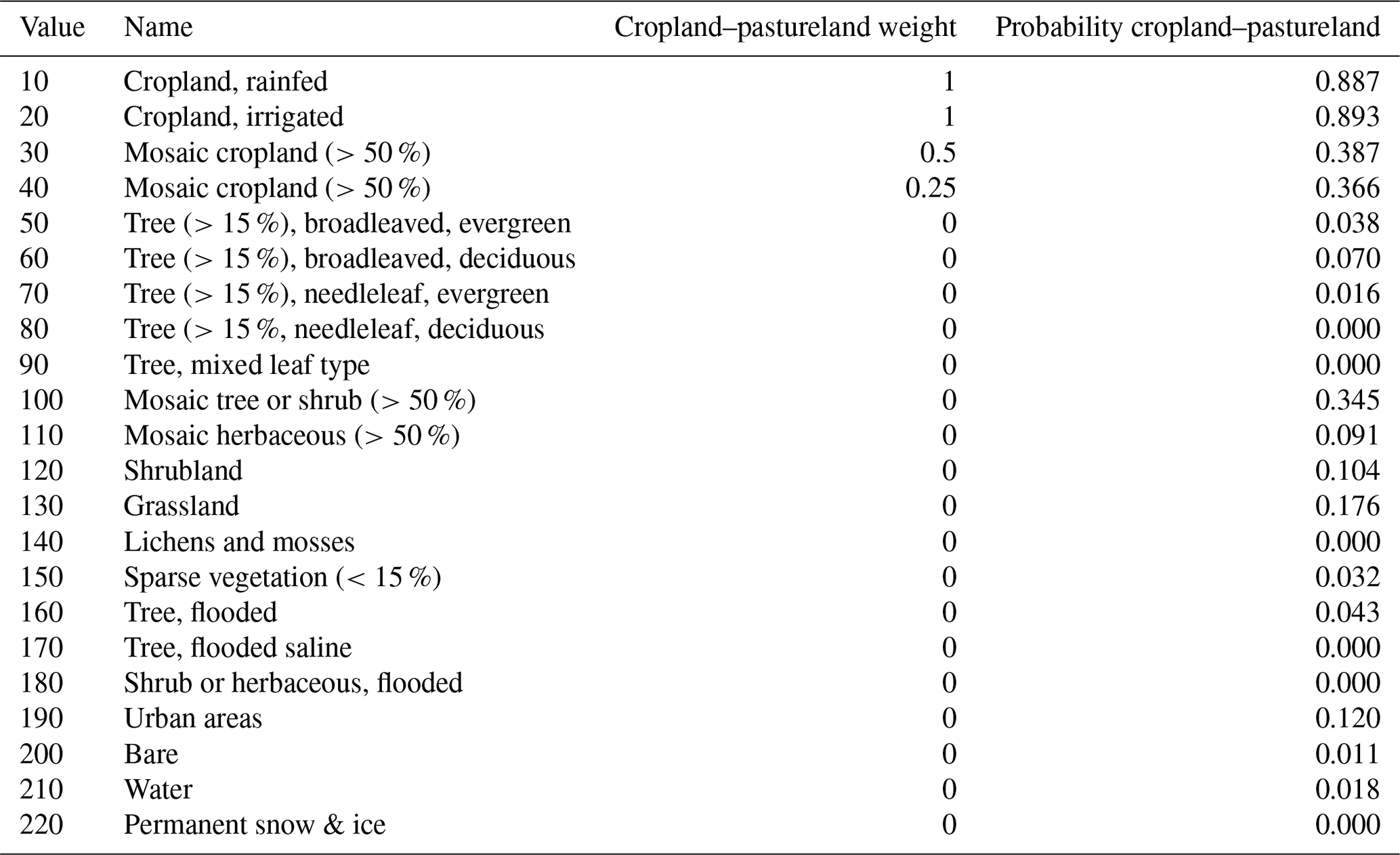
Table 3Probability of a land cover type being classified as cropland or pasture, calculated using the producer's accuracy, which is how often features on the ground are classified or the probability that a certain pixel is classified as a given land cover class. Probabilities of being cropland or pasture cover type (Ccp) are adjusted based on patch size (A) for patches with A<1 km2, where .
2.2.2 Agriculture
We mapped agriculture stressors by identifying land cover classes associated with crop and pastureland from ESA CCI land cover datasets (ESA CCI, 2017; Pérez-Hoyos et al., 2017; Li et al., 2018) available at 0.09 km2 for 1992, 2000, 2010, and 2015. We merged the cropland and pastureland stressors because these two classes are combined in the ESA land cover data and they are challenging to distinguish even at higher resolution (∼30 m; Wickham et al., 2017). To incorporate classification errors associated with all cover classes, we multiplied the footprint Fcp=1.0 with the probability that a pixel with cover class C was found to be cropland or pasture, p(Ccp), by interpreting reported accuracy assessment results (ESA CCI, 2017, in Table 3). To reduce the effects of scattered pixels that have some probability of being mapped as cropland–pastureland (e.g., misclassified pixels of high-elevation tundra or alpine areas), we multiplied p(Ccp) by the proportion of lands estimated to be cropland from the Unified Cropland Layer (Waldner et al., 2016), v, so that
and also reduced the value of p(Ccp)′ based on patch size A, assuming that accuracy declines rapidly with cropland–pastureland small patches (A<1 km2) using
We then calculated Hcp as
We developed spatially explicit estimates of agricultural intensity based on land management, such as cropping and number of rotations, tilling, and cutting operations, because these activities typically vary geographically (van Asselen and Verburg, 2012; Kehoe et al., 2017). We followed existing methods (Chaudhary and Brooks, 2018) to estimate three intensities of agricultural land use – minimal, light, and intense – and then mapped them using cover types from the Global Land Systems v2 dataset (GLS; Kehoe et al., 2017) by estimating intensity values (I) for each of the agricultural intensity types (Table 2). Although GLS v2 represents conditions circa 2005, we incorporated temporal changes by weighting the proportions of agricultural lands from the time-varying ESA CCI land cover datasets.
To estimate the modification associated with the grazing of domestic livestock (Hau), we used Gridded Livestock of the World v3 (Robinson et al., 2014; Gilbert et al., 2018a–i) which maps the density of animals per square kilometer (G) for eight types of livestock (j): buffaloes, cattle, chickens, ducks, goats, horses, pigs, and sheep. To calculate the overall footprint of grazing (Fau), we summed the weighted densities by global averages of livestock unit (LU) coefficients (wi=0.84, 0.67, 0.01, 0.01, 0.10, 0.84, 0.23, 0.10, listed, respectively, for each livestock species stated above). We used a lower threshold found at 10 % to remove values <1.0 LU km−2 (similar to Jacobson et al., 2019) and 1000 LU km−2 as an upper threshold because it is a common breakpoint between grazing and industrial feedlots (Gerber et al., 2010). We assumed (here and below unless otherwise provided) no uncertainty (p(Cau)=1.0), because we lacked explicit data to do so. We then log10 transformed and max-normalized (Kennedy et al., 2019b) to obtain 0–1 values and calculated the mean Hau using a 10 km radius moving window to reduce the effects of the coarser-resolution pixels:
2.2.3 Energy and extractive resources
To estimate stressors associated with extractive energy production, we mapped gas flares derived from nighttime lights using data from the Visible Infrared Imaging Radiometer Suite from the Suomi National Polar-orbiting Partnership (VIIRS; Elvidge et al., 2013). Roughly 90 % of gas flares occur at locations where oil and gas are extracted (Elvidge et al., 2016). We used point data processed specifically to identify gas flares in VIIRS for 2012 and 2013 (Elvidge et al., 2016). For each flare, we approximated a footprint of 0.057 km2 per wellhead (Allred et al., 2015). It is common to approximate the footprint of points (and lines) using a simple “buffer”, which implicitly assumes no location error and no distance decay from the point of origin. Such a buffer approach essentially centers a cylinder on each data point, where volume (V) equals the approximate footprint and height (h) and a perfect certainty of 1.0. Here, however, we assumed some uncertainty in the location of the point and that the effects associated with a feature such as an oil or gas wellhead diminish with distance. That is, rather than use a cylinder with volume V (or similarly a simple uniform buffer away from linear features, e.g., power lines or roads), we used a conic-shaped kernel centered on the point to calculate the uncertainty p(Cog), where the height of the cone h=0.5 represents a conservative estimate of spatial accuracy (Theobald, 2013). We derived the cone radius D=0.329 km by setting V to the footprint of 0.057 km2:
Thereby the uncertainty parameter for each point is calculated using
We assigned the value of p(Cog) that overlapped the center of each pixel, with max p(Cog)=1.0. Human modification was then calculated as
2.2.4 Mines and quarries
To estimate modification due to mines and quarries, we derived locations represented as points from a global mining dataset (n=34 565; S&P, 2018; Valenta et al., 2019). We retained surface mines that were constructed, where construction had started, were in operation, were in the process of being commissioned, or had residual production (n=22 705). For the temporal change analysis, we removed locations that did not have a specified year of construction (n=3634). We calculated the mean disturbed area and associated infrastructure of a mine by intersecting mine point locations with 441 623 polygons that represent footprints of quarries and mines (OpenStreetMap, 2019). For four types of mines – coal, hard rock (bauxite, cobalt, copper, gold, iron ore, lead, manganese, molybdenum, nickel, phosphate, platinum, silver, tin, uranium oxide, and zinc), diamonds, and other (antimony, chromite, graphite, ilmenite, lanthanides, lithium, niobium, palladium, tantalum, and tungsten) – we estimated the mean area (a) to be 12.95 km2 (n=647) for coal, 8.54 km2 (n=860) for hard rock, 5.21 km2 (n=39) for diamonds, and 3.40 km2 (n=27) for other. Finally, following Eqs. (8) and (9), we calculated p(Cm) for each of the four mining types using D values of 4.973, 4.038, 2.548, and 3.154 km, respectively, and calculated Hm as
2.2.5 Power plants
To estimate the effects of where energy is produced, we mapped the location of power plants represented as points (n=29 903; WRI, 2019). For the temporal change analysis, we removed locations that did not have a specified year of construction (n=16 288). We estimated p(Cpp) using a conic-shaped kernel (Eqs. 8 and 9) and h=0.5. We mapped both nonrenewable energy forms (Hppn; coal, oil, natural gas) and renewable energy forms (Hppr; geothermal, hydro, solar, wind), where we assumed Fpp=1 and calculated a single p(Cpp) for both nonrenewable and renewable energy sectors with Dpp=1224 m (following Theobald, 2013):
2.2.6 Transportation and service corridors
For transportation, we mapped roads and railways using OpenStreetMap highway linear features (OpenStreetMap, 2019). We calculated the footprint for the following transportation types: major (motorway, primary, secondary, trunk, link), minor (residential, tertiary, tertiary link), and two-track roads and railways as
where w is the estimated width of a road of type i from Table 2, α is the pixel width (i.e., 300 m), and μ=0.79 to adjust for the fractal dimension of road lines crossing cells (Theobald, 2000) because road lines often cross pixels at random angles. If a divided highway is represented as two separate lines, then each is represented independently. Also, if a cell has two or more roadway types cross it (e.g., where a secondary road joins a highway), the fuzzy sum of Hrr for both roads is calculated. Note that use of roads is incorporated into the “human intrusion” stressor (described below).
To map the modification associated with aboveground power lines (Hpl), we used
where Fpl is calculated using a 500 m buffer (Theobald, 2013), p(Cpl) is calculated using h=0.5, and Ipl is the estimate of intensity.
To estimate a stressor associated with electrical infrastructure and energy use (Hnl), we mapped “nighttime lights” using the Defense Meteorological Satellite Program Operational Linescan System (DMSP OLS; Elvidge et al., 2001) “stable lights” dataset. We included this as a distinct stressor from the energy extraction stressor (oil and gas flares, discussed above) because gas flares are derived by finding anomalies (high values) in the images rather than from the stable lights product and the footprints associated with the flares are an extremely small fraction of the overall extent of energy infrastructure.
To maximize temporal consistency, we used the intercalibrated DMSP OLS dataset and extended their (Zhang et al., 2016; Li and Zhou et al., 2017) approach for 2013 (using a=1.01, b=0.00882, ; Zhang et al., 2016). DMSP OLS values, L, are expected to range from 0 to 63, but because max values differed yearly (ranging from 57.87 to 66.16), we normalized all images (1992–2013) to range from 0 to 1.0 using the max-adjusted value for each year (L′). To reduce the effects of noise in the images in areas with low light and in high northerly latitudes, we removed nighttime light values when – that is, we set values to null when they were below the 25th percentile of the global terrestrial distribution compared to the often-used noise threshold of L=5 (following Elvidge et al., 2001).
To adjust for interannual spatial-misalignment errors (Elvidge et al., 2013), we adjusted the normalized DMSP image for 2013 to align with the 2013 VIIRS product by identifying sharply contrasting and consistent signals at 10 locations (n=10) distributed across the continents. We then visually compared each of the images from 1992 to 2012 to the DMSP image for 2013 and shifted the images to align them (averaged shift in meters – x=359.5, y=476.2). To further reduce interannual variability, we averaged image values at each pixel using a 3-year “tail” and used a rank-ordered-centroid weighting (Roszkowska, 2013) such that the spatially aligned and temporally smoothed nightlight value Y for year t is
Finally, to reduce the blooming effects and to take advantage of the higher-quality VIIRS-based nightlights (i.e., higher spatial resolution, reduction in saturated pixels), we sharpened DMSP nightlight values yt using the VIIRS brightness value y to be proportional to the ratio of the DMSP values:
We then transformed following Kennedy et al. (2019b), capping values above 126.0 (the 99.5 percentile of global values):
2.2.7 Logging
To estimate stressors on forested lands, we used maps of forest loss (Curtis et al., 2018) associated with commodity-driven deforestation, shifting agriculture, and forestry. (Note that we excluded as stressors wildfire because of the challenges of attributing wildfires to human causation – especially over global extent – and urbanization because it is measured directly by the built-up stressor.) We then identified locations where forest was lost due to one of the three mapped stressors (using v1.6, updated to 2018; Hansen et al., 2013) prior to the year of our estimated human modification map and applied the intensity value associated with that stressor. Thus,
where Ffr is pixels of forested loss in a given year and Ifr is an estimate of intensity associated with the cause of forest loss.
2.2.8 Human intrusion
We estimated human intrusion (Hi) using a method that builds on and extends accessibility modeling (Nelson, 2008; Theobald, 2008, 2013; Theobald et al., 2010; Weiss et al., 2018; Nelson et al., 2019). Human intrusion (a.k.a. “use”; Theobald, 2008) uses central place theory (Alonso, 1960) and integrates human accessibility throughout a landscape from defined locations, typically along roads and rails, as well as to off-road areas from urban areas (Theobald et al., 2010; Esteves et al., 2011; Theobald, 2013; Larson et al., 2018).
Accessibility measured in travel time in minutes is calculated from each mapped settlement point j (e.g., cities, towns, villages) from GRUMP v1.01 and GPW v4 (CIESIN, 2017, 2018). This approach is much less sensitive to arbitrary thresholds of city or town size (e.g., 50 000 residents), often used due to computational constraints (e.g., Nelson, 2008; Weiss et al., 2018). Second, to estimate intrusion of people into adjacent areas from a given settlement, we estimated the number of people (using population estimates at settlement j) at a given location (X; population density is people per square kilometer) following the assumption that the human density halved with every 60 min traveled (Theobald, 2008, 2013). The resulting intrusion map for each settlement was then summed to account for typical overlaps of intrusion from nearby settlements. We assumed that there is a limit at very high population densities, and so we capped the maximum value of intrusion, X, at 1 000 000 and then max-normalized using a square-root transform:
Note that accessibility was calculated using estimates of travel time along roads and rails, as well as off-road through different features of the landscape, using established travel time factors (Tobler, 1991) and presuming walking off-trail or via boats on freshwater or along ocean shoreline (Nelson, 2008; Theobald et al., 2010; Weiss et al., 2018; Nelson et al., 2019). This included effects of international borders following Weiss et al. (2018), and accessibility to lands was calculated across oceans.
2.2.9 Natural systems modification
Dams and their associated reservoirs flood natural habitat and strongly impact the natural flow regimes of the adjacent rivers (Grill et al., 2019). We mapped the footprint of reservoirs Fr created from 6849 dams from the Global Reservoir and Dam database (GRanD v1.3; Lehner et al., 2011; http://globaldamwatch.org/grand/, last access: 28 December 2019).
Because there are some potential analyses that would benefit from treating all water bodies consistently, we provided an additional version with all water bodies masked out in the dataset.
2.2.10 Pollution
We estimated the stress of air pollution by using data on nitrogen oxides (NOx) through time from the Emission Database for Global Atmospheric Research (EDGAR v4.3.2; Crippa et al., 2018). We selected NOx because it is a strong contributor to acid rain and fog and tropospheric ozone and because atmospheric levels are predominantly from human sources (Delmas et al., 1997). We used the 99th percentile (46 750 Mt) as the maximum value and then max-normalized (Fnox) and adjusted using the intensity value Inox:
2.3 Uncertainty and validation analyses
To understand the uncertainty in our results associated with our estimated intensity values (Table 2), following Kennedy et al. (2019c), we recalculated H, where Is was randomized (n=50) between the minimum and maximum intensity values for each stressor. We then calculated the per-pixel mean and standard deviation for the 50 randomizations at 1 km2 resolution for computational efficiency and provided corresponding maps.
We also assessed the accuracy of our maps following validation procedures described in Kennedy et al. (2019a, b, c). Because historical ground truth human modification data in a comparable form are not widely available, we restricted our analysis to test the contemporary conditions of human modification (∼2017 map) that included all stressor layers. We used an independent validation dataset from Kennedy et al. (2019b) that quantified the degree of human modification from visual interpretation of high-resolution aerial or satellite imagery across the world. We selected plots using the Global Grid sampling design (Theobald, 2016), a spatially balanced and probability-based random sampling that was stratified on a five-class rural-to-urban gradient using stable nighttime lights 2013 imagery (Elvidge et al., 2001). Within each of the 1000 ∼1 km2 plots, we selected 10 simple random locations to capture rare features and heterogeneity in land use and land cover (for a total of 10 000 subplots), which were separated by a minimum distance of 100 m. The spatially balanced nature of the design maximizes statistical information extracted from each plot, because it increases the number of samples in relatively rare areas that are likely of interest (in contrast to simple random sampling) – especially for urbanized and growing cities (Theobald, 2016).
2.4 Processing platform
We processed, modeled, and analyzed the spatial data using the Google Earth Engine platform (Gorelick et al., 2017). We calculated all distances and areas using geodesic algorithms in decimal degrees (EPSG 4326). We summarized areas and percentages after projecting the data to the Mollweide equal-area projection (WGS84) to simplify calculations. All datasets and maps conform to the Google Earth Engine terms of service. We used program R 3.6.1 (R Core Team, 2019) to generate Fig. 2.
Table 4Summary of estimates of the degree of human modification (H) and the mean annualized difference between 5- or 10-year increments for which change over time can be calculated (1990, 2000, 2010, and 2015) and H values for the contemporary dataset (∼2017, all stressors). Mean annualized mean difference is calculated as the mean value across the continents of the difference in H values divided by the number of years (e.g., ).
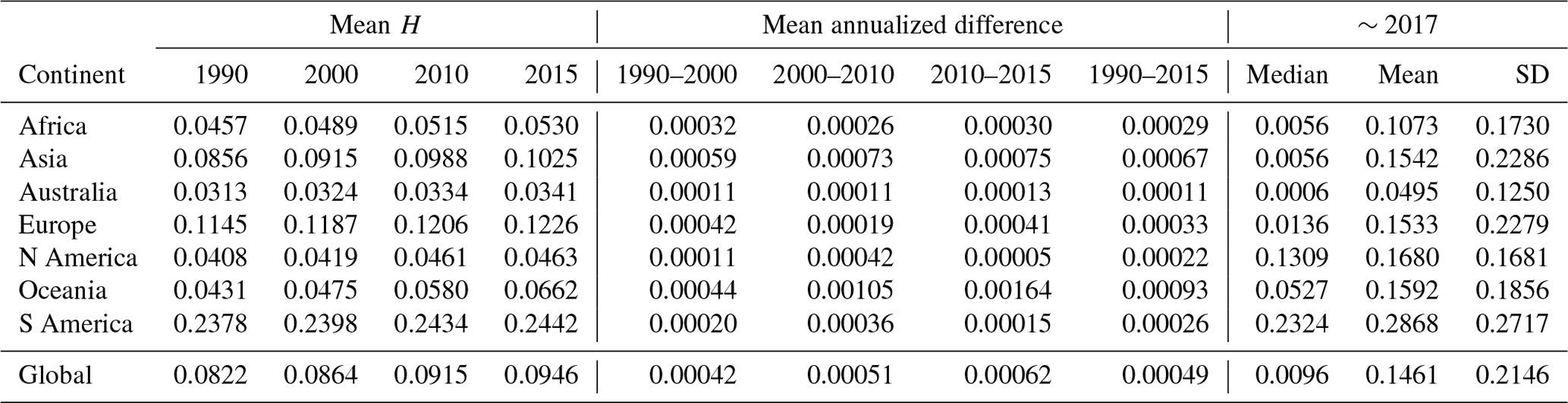
Table 5A comparison of the mean annualized difference in human modification values for changes from 1990 to 2015 (H; 1990–2015), human footprint (HF; 1993–2009; Venter et al., 2016), and the temporal human pressure index (THPI; 1995–2010; Geldmann et al., 2019b). Mean annualized mean difference is calculated as the mean value of the difference in H values divided by the number of years (e.g., ), for each continent. Note that Oceania extends below Papua New Guinea (excluding the country of Australia).

Below we describe the temporal and spatial trends of human modification by continent (Table 4), biome (Table 5), and ecoregion (Fig. 2).
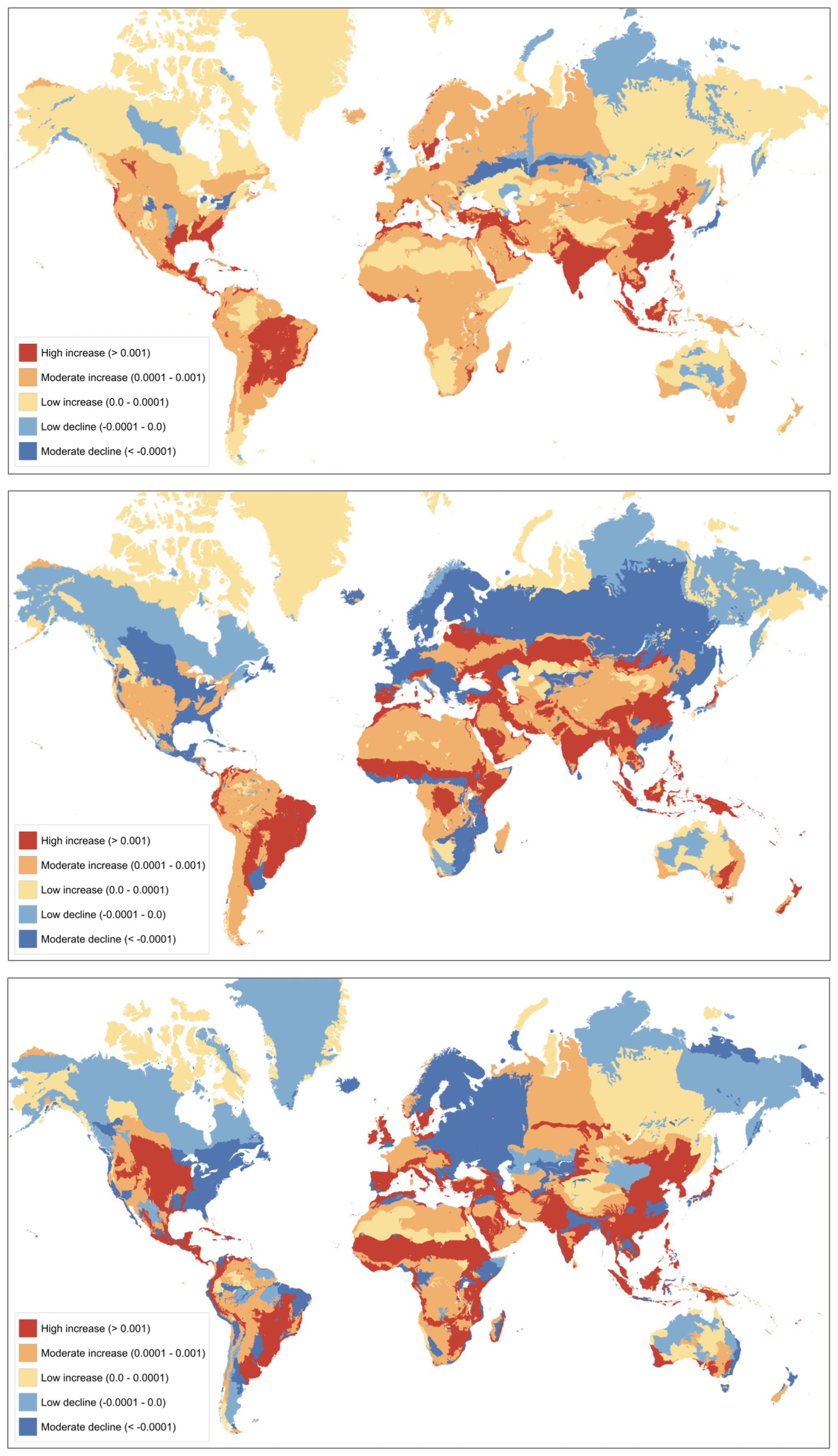
Figure 1A comparison of the recent trends in human activities by ecoregion using the mean annualized difference estimated by (a) human modification (H; from 1990 to 2015), (b) human footprint (for 1993–2009; Venter et al., 2016), and (c) temporal human pressure index (for ∼1995–2010; Geldmann et al., 2019a). Note that interactive maps are available at https://davidtheobald8.users.earthengine.app/view/global-human-modification-change (last access: 29 August 2020).
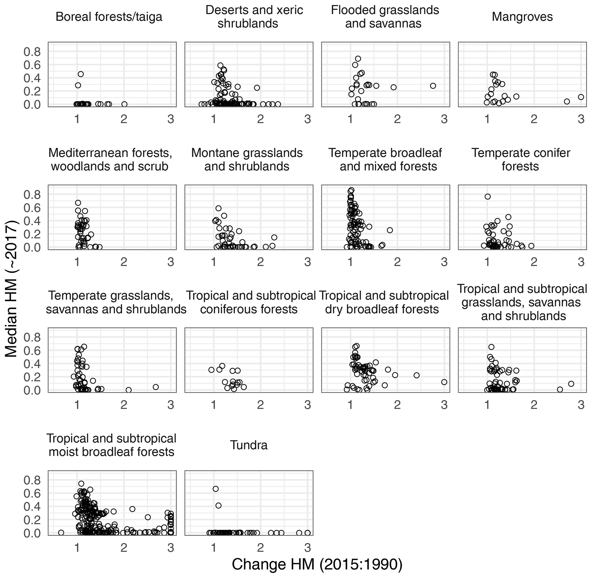
Figure 2Graphs of the ratio of natural land loss (2015:1990) and contemporary (∼2017) degree of human modification (denoted as HM) for each of the 14 biomes and their ecoregions, globally. Note that ecoregions with change ratios ≥3.0 are placed on the maximum x-axis value (3.0).
3.1 Changes from 1990 to 2015
The mean value of H for global terrestrial lands increased from 0.0822 in 1990 to 0.0946 in 2015, a percentage change of 15.04 % overall and 0.60 % annually (Table 4). This equates to 1.6 M km2 of natural lands lost – 178 km2 daily. Increases in human modification occurred globally and in both urban and rural locations. We found that the largest increases in the Hmad occurred in Oceania, followed by Asia and Europe. Australia had the lowest increase followed by North and South America (Table 4). The biomes that exhibited the greatest increases in modification were mangroves, tropical and subtropical moist broadleaf forests, and tropical and subtropical dry broadleaf forests, while the biomes with the smallest increases were tundra, boreal forests and taiga, and deserts and xeric shrublands. Maps of changes in the Hmad between 2015 and 1990 for each ecoregion are shown in Fig. 1a, relative to the HF (Fig. 1b) and THPI (Fig. 1c). Figure 2 shows the ratio of natural land loss between 1990 and 2015, for each ecoregion and grouped by biome, in the context of the contemporary extent of human modification. We found most ecoregions (n=814) had increased in human modification, while the few (n=32) that had decreased were concentrated in higher latitudes and in more remote areas. We also found that changes in the Hmad have increased over time, from 0.0004 to 0.0005 to 0.0006, during 1990–2000 to 2000–2010 to 2010–2015. The percent change has also increased over time from 0.51 % to 0.59 % to 0.68 %.
3.2 Contemporary extent
We found that about 19.1 M km2 (±0.0013) of natural lands was lost by ∼2017 – about 14.6 % of land globally (Table 4). South America was the most transformed (28.7 %), followed by North America (16.8 %), while Australia (5.0 %) and Africa (10.7 %) were the least transformed. Broad-scale patterns of the extent of human modification in ∼2017 are shown in Fig. 3. Note that “natural lands lost” was calculated using the continuous value of H, rather than approximations based on classifying the distribution.
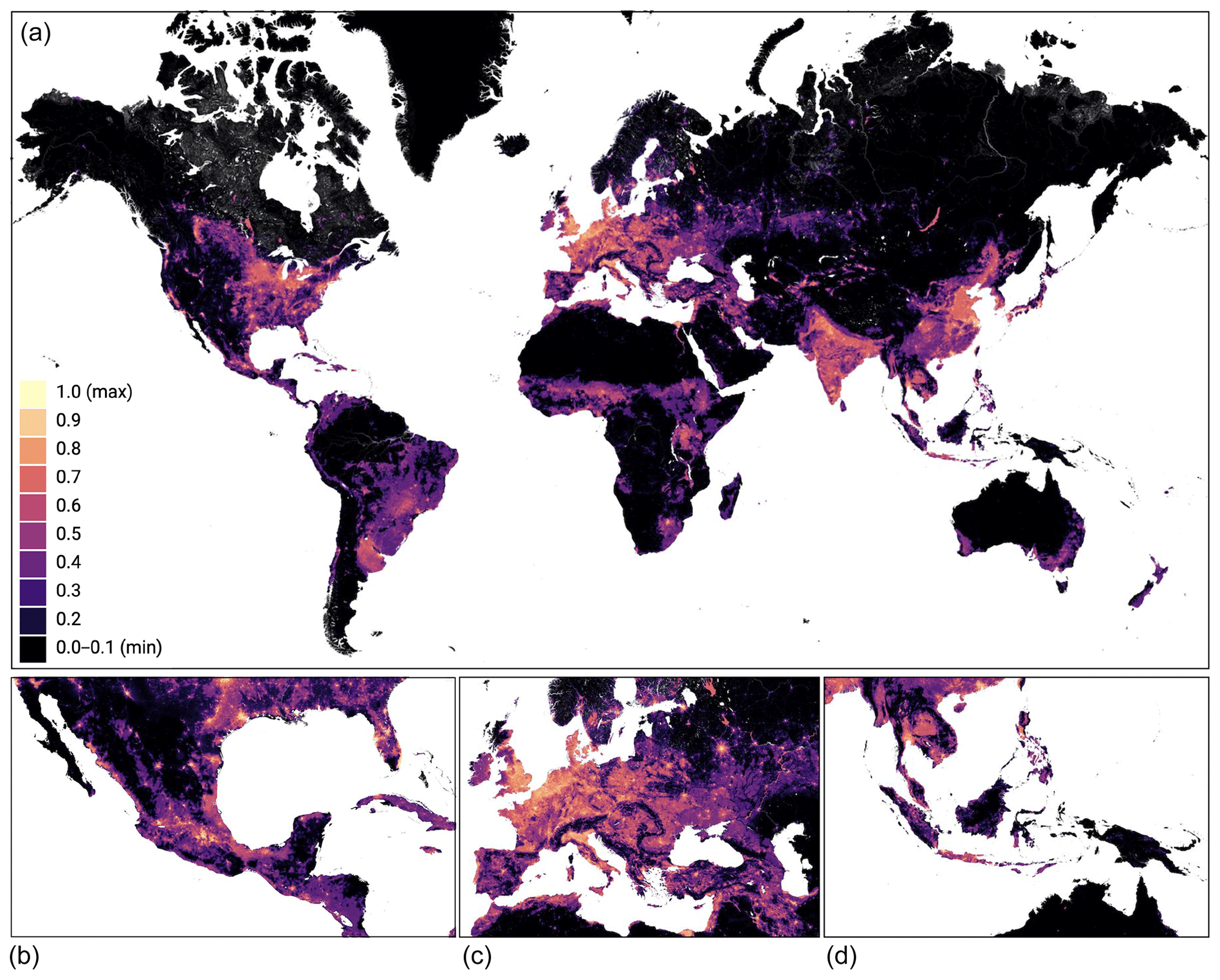
Figure 3The degree of human modification for circa ∼2017: (a) globally; (b) in central America; (c) in Europe, and (d) in Oceania. Note that interactive maps are available at https://davidtheobald8.users.earthengine.app/view/global-human-modification-change (last access: 29 August 2020).
Terrestrial lands with very low levels of human modification (H<0.01; Kennedy et al., 2019a; Riggio et al., 2020) are concentrated in less productive and more remote areas in high latitudes and are dominated by inaccessible permanent rock and ice or are within tundra, boreal forests, desert regions, and to a lesser extent montane grasslands. Table 5 shows that the biomes with the highest levels of H in ∼2017 were temperate broadleaf and mixed forests (H=0.3744); tropical and subtropical dry broadleaf forests (H=0.3317); and Mediterranean forests, woodlands and scrub (H=0.2903). The five least modified biomes were tundra (mean H=0.0023), boreal forests and taiga (H=0.0213), deserts and xeric shrublands (H=0.0572), and montane grasslands and shrublands (H=0.0894).
Following thresholds from Kennedy et al. (2019b), we found that in ∼2017, 51.0 % of global lands had a mean value of H≤0.01 (i.e., very low human modification), 13.3 % had a mean of (low), 21.0 % had a mean of (i.e., moderate), 12.3 % had a mean value of (high), and 2.4 % (3.2 M km2, ±0.0003) had a mean of (very high). By area, these results by class amount to the following: very low = 66.8 M km2 (±0.0067), low = 17.4 M km2 (±0.0017), moderate = 27.6 M km2 (±0.0028), high = 16.1 M km2 (±0.0016), and very high = 3.18 M km2 (±0.0003). Also, we found that 17.6 % had a mean value of H<0.0001 (23.0 M km2, ±0.0023) and 4.2 % had H<0.00001 (5.5 M km2, ±0.0006).
Table 6A summary of the data, methods, and results comparing the degree of human modification (HM; this paper), degree of human modification 1 km (HM1k; Kennedy et al., 2019a, b, c), human footprint (HF; Sanderson et al., 2002; Venter et al., 2016), and temporal human pressure index (THPI; Geldmann et al., 2019b). Also see discussion of comparison in Kennedy et al. (2019a, c), Venter et al. (2019), and Riggio et al. (2020). Data source acronyms are provided in Table 1.
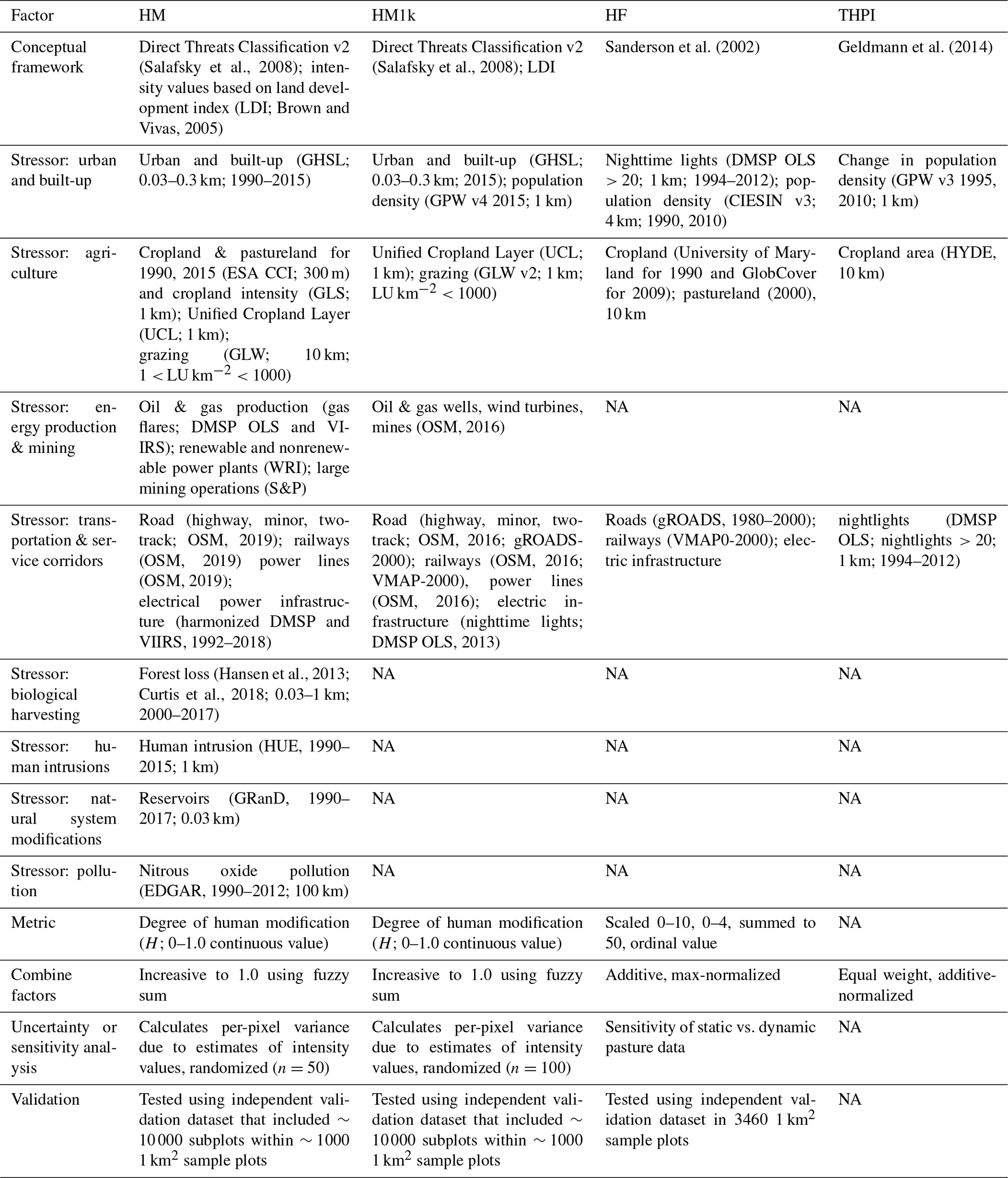
NA: not available
3.3 Comparisons
We compared our work to earlier efforts (summarized in Table 6) to determine if overall trends and extents were generally consistent with similar priorities of biomes and ecoregions. Globally, the Hmad from 1990 to 2015 (t=1990, u=2015) was 0.0005, while for the HF and THPI it was higher (HFmad=0.0006, THPImad=0.0008). Perhaps more important is that the variability of the mean annualized difference values in the HF and THPI was 2.3 and 3.2 times that of H. By continent, we found that the Hmad increased the most in Oceania, followed by Asia, Europe, Africa, South America, North America, and Australia. Continental ranks by the THPI followed H roughly, though the HF differed more substantially (Table 5). The Hmad increased for all continents, but the HFmad showed declines in modification for Europe and South America, while the THPImad showed a decline for North America.
Table 7Summary of results by biome, comparing trends using the mean annualized difference for the human modification (Hmad), human footprint (HFmad; Venter et al., 2016), and the mean temporal human pressure index (THPImad; Geldmann et al., 2019) score. Also provided are estimates of the proportion of terrestrial lands modified as estimated from Kennedy et al. (2018, 2019b; H1k) and the HF (score was max-normalized to rescale to 0–1). The THPI dataset characterizes only change, and so estimates of the proportion of lands modified in 2010 could not be provided. Mean annualized mean difference is calculated as the mean value across the continents and globally of the difference in H values divided by the number of years.
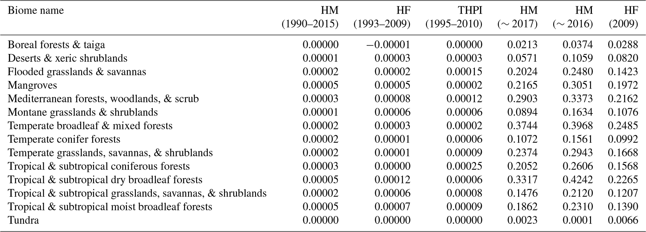
We also found the ranking of biomes by mean annualized difference for the HF and THPI was fairly different from ranks developed from H values (Table 7). Of the three biomes with the largest increase for the Hmad, two were also identified by the HF (tropical and subtropical dry broadleaf forests and tropical and subtropical moist broadleaf forests) and none by the THPI. Of the five biomes with the largest increase for the Hmad, three were also identified by the HF and THPI. The biomes that had the greatest disagreement among the ranking of H, the HF, and the THPI were mangroves, tropical and subtropical coniferous forests, and tropical and subtropical dry broadleaf forests.
The biggest differences in rankings between the H and the HF were for temperate and broadleaf mixed forests (and see comparisons of H1k and the HF in Kennedy et al., 2019b, c; Riggio et al., 2020). The HF was estimated to result in a 12.3 % modification for an earlier date (∼2009; Venter et al., 2016) and is lower likely because fewer stressors were included, because of its additive combination method, and because of its strongly right-skewed distribution caused by max-value normalization. The ranks of the extent of modification by biomes, however, were very similar in H, H1k, and the HF. In general, H had intermediate modification levels compared to H1k and the HF, with H1k levels being slightly higher (difference between 0.00 min and 0.09 max and average difference of 0.05 by biome) and the HF being slightly lower (difference between 0.00 min and 0.13 max and average difference of 0.04 by biome; Table 7). Results for ecoregions shown in Fig. 1 are even more striking, as the mean annualized difference values for the HF and THPI were inconsistent with our results. Of the 814 ecoregions that had increases in the Hmad, a decrease in modification was found for 201 ecoregions for the HFmad and 202 for the THPImad; and for the 32 ecoregions that were found to have decreases in the Hmad, an increase in modification was found for 20 in the HF and 22 in the THPI.
Finally, the global estimate for H1k was likely higher than H because H1k did not limit the livestock stressor at LU km−2 <1.0, used a slightly higher value for the low-threshold on the electrical infrastructure and energy use stressor (i.e., nightlights), and reported results that incorporate uncertainty into estimates of intensity. Furthermore, global modification from farming was estimated at 37 % for 2000 (Ramankutty et al., 2008) compared to 14.6 % with H. The difference with our results is largely due to their (Ramankutty et al., 2008) mapping of the area land cover types without differentiating the intensity of the impact of those cover types (crop and pasture).
3.4 Uncertainty and validation analyses
We addressed uncertainty in our results by incorporating the parameter p(Cs) for every sector s to best quantify uncertainty in its spatial location and classification as detailed in Sect. 2.2; for example, we adjusted p(Ccp) by directly incorporating measured confusion among land cover types using the results from the accuracy assessment of the land cover dataset (from Eq. 4). Additionally, we incorporated uncertainty by calculating the global mean for each of the 50 randomizations, which across the 50 iterations was 0.1434 () and ranged from 0.1243 to 0.1612. Thus, the global mean of 0.1461 obtained using our best-estimate intensity values was in line with our uncertainty results. We also mapped the per-pixel variance (standard deviation) to examine the spatial pattern of uncertainty (Fig. 4). The locations of the highest levels of uncertainty tend to be in more highly developed landscapes.
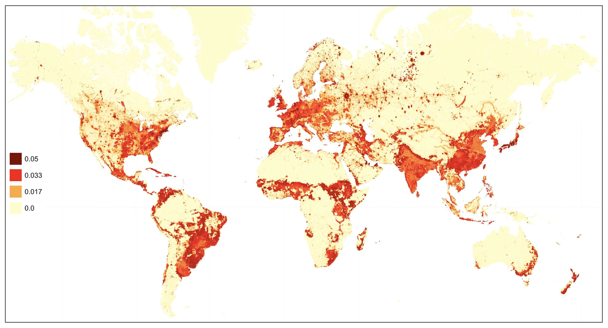
Figure 4A map of the uncertainty as a result of randomizing the intensity factors when calculating the degree of human modification for 2017, showing the per-pixel standard deviation of 50 randomized maps. The highest levels of uncertainty tend to be in more highly developed landscapes (minimum = 0.0, median = 0.0, mean = 0.009, standard deviation = 0.014, maximum = 0.186).
We found strong agreement between H for ∼2017 and our validation data (r=0.783), with an average root mean square error of 0.22 and a mean absolute error of 0.04, for the 926 ∼1 km2 plots (9260 subplots). There were 726 plots within ±20 % agreement, while for 161 plots H was estimated to be higher (and for 39 plots lower) than our visual estimate from the validation data. Estimates of H were biased high, likely because the stressors for human intrusion and electrical infrastructure (based on nighttime lights) are not readily observable from the aerial imagery used to generate the validation data. Our results here are consistent with our earlier findings (Kennedy et al., 2019a, b, c).
The datasets generated from this work are available at https://doi.org/10.5281/zenodo.3963013 (Theobald et al., 2020), which includes the land–water mask used to support subsequent analyses. Extracts of specific geographic areas can be obtained by contacting the authors. All other datasets used in our work are open-source data cited herein.
5.1 Summary
We found rapid and increasing human modification of terrestrial systems, resulting in the loss of natural lands globally. Our findings foreshadow trends and patterns of increased human modification, assuming future trends in the next 25–30 years continue as they have recently. Thus, our study reinforces calls for stronger commitments to help reduce habitat loss and fragmentation (Kennedy et al., 2019b; Jacobson et al., 2019) – which should be considered in conjunction with current commitments to reduce CO2 emissions through the Paris climate accord (Baruch-Mordo et al., 2019; Kiesecker et al., 2019). We believe that the comparisons of ecoregions and biomes offer valuable contextual information that provides initial guidance on conservation strategies that may be most appropriate (Kennedy et al., 2019b). Also, it is important to consider the feasibility of achieving ecoregional (Dinerstein et al., 2017) or ecosystem (Jantke et al., 2019) representation goals as well as additional stresses caused by climate change (Costanza and Terando, 2019). We emphasize that although global, continental, biome, and ecoregional summaries provide a general understanding of trends and patterns, the high resolution of H and its gradient nature support robust estimates of change in human modification within a country and within an ecoregion, which are essential for tracking progress toward international and national conservation commitments (Mace et al., 2018), especially when placed within a broader structured decision-making framework (Tulloch et al., 2015).
Our datasets of human modification provide the most granular, contemporary, comprehensive, high-quality, and robust data currently available to assess temporal and spatial trends of global human impacts on landscapes. Our work is grounded in a structured classification of stressors, uses an internally consistent model, evaluates uncertainty, and incorporates refinements to minimize the effects of scaling and classification errors. Our validation approach uses an independent and spatially balanced random-sample design to provide strong support for the quality of our findings (Kennedy et al., 2019a).
Our overarching goal in producing and publishing these datasets is to support detailed quantification of the rates and trends, as well as the current extent and pattern, of human modification and to understand the degree of human modification across the continuum from low (e.g., wilderness) to high (e.g., intense urban). Beyond the basic findings presented here, we believe there are many potential applications of these datasets, including examining temporal rates and trends of land modification in and around protected areas (e.g., Geldmann et al., 2019b), estimating fragmentation for ecoregions and biomes (Kennedy et al., 2019b; Jacobson et al., 2019), and evaluating conservation opportunities and risks (e.g., the conservation risk index; Hoekstra et al., 2005). We also note that the human modification approach allows, in a straightforward and logically consistent way, for the inclusion of additional stressors and higher-resolution datasets that may become available over time or may be available for specific, local areas.
5.2 Caveats
As with any model, we recognize there are limitations to our work. We did not include data for all human stressors, largely because of incomplete global coverage or coarse mapping units (Klein Goldewijk et al., 2007; Geldmann et al., 2014), an inability to discern human-induced versus natural disturbances, or uncertainty in the location and directionality of their impact (e.g., the impact of climate change on terrestrial systems; Geldmann et al., 2014). In particular and discussed in Kennedy et al. (2019b, c), changes to land cover due to ecological disturbance events, such as wildfires or flooding, are not included in our analysis because of the difficulty in separating natural from human-caused disturbances – yet, we recognize that the broad extent of wildfire in particular could have strong implications. We did not include climate data as a stressor in this product to keep our analysis manageable and tractable. Although we attempted to map each stressor comprehensively, we recognize that some datasets may have missing features, particularly for mine and oil/gas wells – though large mines and concentrated oil/gas fields have been mapped quite well. For more integrated analyses, our data product should be used in combination with datasets of impacts due to climate change (e.g., Parks et al., 2020).
Stressors that are particularly important to improve include effects of grazing (currently coarse data and very broad expanse), pasture land, invasive species, and climate change (especially wildfire and effects of sea-level rise), and we encourage future work to focus on developing appropriate datasets and approaches to include or better capture these stressors. Key datasets we believe should be improved include transportation networks, including logging roads (e.g., van Etten, 2019), that are comparable through time; livestock grazing, rangelands, croplands, timber plantations, and pasturelands and their intensity of use; resource extraction (especially mining footprints); and temporal trends in gas flares, utility-scale solar and wind installations (Dunnett et al., 2020), and electrical substations.
DMT, CK, BC, JO, SBM, and JK conceived the paper; DMT, CK, JO, and BC prepared data; DMT implemented the model; DMT, CK, BC, and SBM conducted summary analyses; DMT, CK, BC, JO, SBM, and JK developed recommendations; all contributed to writing the manuscript.
The authors declare that they have no conflict of interest.
We thank OpenStreetMap contributors (copyright OpenStreetMap and data are available from https://www.openstreetmap.org, last access: 8 October 2019), and Eleonore Lebre for assistance with the global mining data.
This paper was edited by David Carlson and reviewed by three anonymous referees.
Allred, B. W., Smith, W. K., Tidwell, D., Haggerty, J. H., Running, S. W., Naugle, D. E., and Fuhlendorf, S. D.: Ecosystem services lost to oil and gas in North America, Science, 348, 401–402, 2015.
Alonso, W.: A theory of the urban land market, Papers in Regional Science, 6, 149–157, 1960.
Baruch-Mordo, S., Kiesecker, J., Kennedy, C. M., Oakleaf, J. R., and Opperman, J. J.: From Paris to practice: sustainable implementation of renewable energy goals, Environ. Res. Lett., 14, 1–8, https://doi.org/10.1088/1748-9326/aaf6e0, 2019.
Bonham-Carter, G. F.: Geographic information systems for geoscientists: modelling with GIS (Vol. 13), Elsevier, Tarrytown, New York, 1994.
Brown, M. T. and Vivas, M. B.: Landscape development intensity index, Environ. Monitor. Assess., 101, 289–309, 2005.
Chaudhary, A. and Brooks, T. M.: Land use intensity-specific global characterization factors to assess product biodiversity footprints, Environ. Sci. Technol., 52, 5094–5104, 2018.
CIESIN: Global Rural-Urban Mapping Project, Version 1 (GRUMPv1): Settlement Points, Revision 01, Palisades, NY: NASA Socioeconomic Data and Applications Center (SEDAC), https://doi.org/10.7927/H4BC3WG1, 2017.
CIESIN: Gridded Population of the World, Version 4 (GPWv4): Administrative Unit Center Points with Population Estimates, Revision 11, Palisades, NY: NASA Socioeconomic Data and Applications Center (SEDAC), https://doi.org/10.7927/H4BC3WMT, 2018.
Corbane, C., Florczyk, A., Pesaresi, M., Politis, P., and Syrris, V.: GHS built-up grid, derived from Landsat, multitemporal (1975–1990–2000–2014), R2018A. European Commission, Joint Research Centre (JRC), https://doi.org/10.2905/jrc-ghsl-10007, 2018.
Costanza, J. K. and Terando, A. J.: Landscape Connectivity Planning for Adaptation to Future Climate and Land-Use Change, Current Landscape Ecology Reports, 4, 1–13, 2019.
Crippa, M., Guizzardi, D., Muntean, M., Schaaf, E., Dentener, F., van Aardenne, J. A., Monni, S., Doering, U., Olivier, J. G. J., Pagliari, V., and Janssens-Maenhout, G.: Gridded emissions of air pollutants for the period 1970–2012 within EDGAR v4.3.2, Earth Syst. Sci. Data, 10, 1987–2013, https://doi.org/10.5194/essd-10-1987-2018, 2018.
Curtis, P. G., Slay, C. M., Harris, N. L., Tyukavina, A., and Hansen, M. C.: Classifying drivers of global forest loss, Science, 361, 1108–1111, 2018.
Delmas, R., Serca, D., and Jambert, C.: Global inventory of NOx sources, Nutr. Cycl. Agroecosys., 48, 51–60, 1997.
Dinerstein, E., Olson, D., Joshi, A., Vynne, C., Burgess, N. D., Wikramanayake, E., Hahn, N., Palminteri, S., Hedao, P., Noss, R., and Hansen, M.: An ecoregion-based approach to protecting half the terrestrial realm, BioScience, 67, 534–545, 2017.
Dinerstein, E., Vynne, C., Sala, E., Joshi, A. R., Fernando, S., Lovejoy, T. E., and Burgess, N. D.: A Global Deal For Nature: Guiding principles, milestones, and targets, Sci. Adv., 5, eaaw2869, https://doi.org/10.1126/sciadv.aaw2869, 2019.
Doll, C. N.: CIESIN thematic guide to night-time light remote sensing and its applications. Center for International Earth Science Information Network of Columbia University, Palisades, NY, 2008.
Dunnett, S., Sorichetta, A., Taylor, G., and Eigenbrod, F.: Harmonised global datasets of wind and solar farm locations and power, Sci. Data, 7, 1–12, 2020.
Ellis, E.: Anthropocene: A very short introduction, Oxford University Press, Oxford, UK, 2018.
Ellis, E. C. and Ramankutty, N.: Putting people in the map: anthropogenic biomes of the world, Front. Ecol. Environ., 6, 439–447, 2008.
Elvidge, C. D., Imhoff, M. L., and Baugh, K. E.: Night-time lights of the world: 1994–1995, ISPRS J. Photogramm. Remote S., 56, 81–99, 2001.
Elvidge, C., Ziskin, D., Baugh, K., Tuttle, B., Ghosh, T., Pack, D., Erwin, E., and Zhizhin, M.: A Fifteen Year Record of Global Natural Gas Flaring Derived from Satellite Data, Energies, 2, 595, https://doi.org/10.3390/en20300595, 2009.
Elvidge, C. D., Baugh, K. E., Zhizhin, M., and Hsu, F. C.: Why VIIRS data are superior to DMSP for mapping nighttime lights, Proceedings of the Asia-Pacific Advanced Network, 35, 62–69, 2013.
Elvidge, C., Zhizhin, M., Baugh, K., Hsu, F. C., and Ghosh, T.: Methods for global survey of natural gas flaring from visible infrared imaging radiometer suite data, Energies, 9, 14, https://doi.org/10.3390/en9010014, 2016.
ESA CCI: Land Cover CCI Product User Guide v2 (CCI-LC-PUGv2), Table 3–6, Universite catholique de Louvain, Louvain, Belgium, 2017.
Esteves, C. F., de Barros Ferraz, S. F., de Barros, K. M., Ferraz, M. G., and Theobald, D. M.: Human accessibility modelling applied to protected areas management, Natureza Conservacao, 9, 232–923, 2011.
Gardner, R. H. and Urban, D. L.: Neutral models for testing landscape hypotheses, Landscape Ecol., 22, 15–29, 2007.
Geldmann, J., Joppa, L. N., and Burgess, N. D.: Mapping change in human pressure globally on land and within protected areas, Conserv. Biol., 28, 1604–1616, 2014.
Geldmann, J., Joppa, L., and Burgess, N. D.: Temporal Human Pressure Index, v2, Dryad, Dataset, https://doi.org/10.5061/dryad.p8cz8w9kf, 2019a.
Geldmann, J., Manica, A., Burgess, N. D., Coad, L., and Balmford, A.: A global-level assessment of the effectiveness of protected areas at resisting anthropogenic pressures, P. Natl. Acad. Sci. USA, 116, 23209–23215, 2019b.
Gerber, P., Mooney, H. A., Dijkman, J., Tarawal, S., and De Haan, C.: Livestock in a Changing Landscape, Volume 2: Experiences and Regional Perspectives, Island Press, Washington, D.C., 2010.
Gilbert, M., Nicolas, G., Cinardi, G., Van Boeckel, T. P., Vanwambeke, S. O., Wint, G. W., and Robinson, T. P.: Global distribution data for cattle, buffaloes, horses, sheep, goats, pigs, chickens and ducks in 2010, Sci. Data, 5, 180227, https://doi.org/10.1038/sdata.2018.227, 2018a.
Gilbert, M., Nicolas, G., Cinardi, G., Van Boeckel, T. P., Vanwambeke, S., Wint, W. G. R., and Robinson, T. P.: Global sheep distribution in 2010 (5 minutes of arc), Harvard Dataverse, V3, https://doi.org/10.7910/DVN/BLWPZN, 2018b.
Gilbert, M., Nicolas, G., Cinardi, G., Van Boeckel, T. P., Vanwambeke, S., Wint, W. G. R., and Robinson, T. P.: Global pigs distribution in 2010 (5 minutes of arc), Harvard Dataverse, V3, https://doi.org/10.7910/DVN/33N0JG, 2018c.
Gilbert, M., Nicolas, G., Cinardi, G., Van Boeckel, T. P., Vanwambeke, S., Wint, W. G. R., and Robinson, T. P.: Global horses distribution in 2010 (5 minutes of arc), Harvard Dataverse, V3, https://doi.org/10.7910/DVN/7Q52MV, 2018d.
Gilbert, M., Nicolas, G., Cinardi, G., Van Boeckel, T. P., Vanwambeke, S., Wint, W. G. R., and Robinson, T. P.: Global goats distribution in 2010 (5 minutes of arc), Harvard Dataverse, V3, https://doi.org/10.7910/DVN/OCPH42, 2018e.
Gilbert, M., Nicolas, G., Cinardi, G., Van Boeckel, T. P., Vanwambeke, S., Wint, W. G. R., and Robinson, T. P.: Global ducks distribution in 2010 (5 minutes of arc), Harvard Dataverse, V3, https://doi.org/10.7910/DVN/ICHCBH, 2018f.
Gilbert, M., Nicolas, G., Cinardi, G., Van Boeckel, T. P., Vanwambeke, S., Wint, W. G. R., and Robinson, T. P.: Global cattle distribution in 2010 (5 minutes of arc), Harvard Dataverse, V3, https://doi.org/10.7910/DVN/GIVQ75, 2018g.
Gilbert, M., Nicolas, G., Cinardi, G., Van Boeckel, T. P., Vanwambeke, S., Wint, W. G. R., and Robinson, T. P.: Global chickens distribution in 2010 (5 minutes of arc), Harvard Dataverse, V3, https://doi.org/10.7910/DVN/SUFASB, 2018h.
Gilbert, M., Nicolas, G., Cinardi, G., Van Boeckel, T. P., Vanwambeke, S., Wint, W. G. R., and Robinson, T. P.: Global buffaloes distribution in 2010 (5 minutes of arc), Harvard Dataverse, V3, https://doi.org/10.7910/DVN/5U8MWI, 2018i.
González-Abraham, C., Ezcurra, E., Garcillán, P. P., Ortega-Rubio, A., Kolb, M., and Creel, J. E. B.: The human footprint in Mexico: physical geography and historical legacies, PloS ONE, 10, e0121203, https://doi.org/10.1371/journal.pone.0121203, 2015.
Gorelick, N., Hancher, M., Dixon, M., Ilyushchenko, S., Thau, D., and Moore, R.: Google Earth Engine: Planetary-scale geospatial analysis for everyone, Remote Sens. Environ., 202, 18–27, 2017.
Grill, G., Lehner, B., Thieme, M., Geenen, B., Tickner, D., Antonelli, F., and Macedo, H. E.: Mapping the world's free-flowing rivers, Nature, 569, 215–221, 2019.
Haddad, N. M., Brudvig, L. A., Clobert, J., Davies, K. F., Gonzalez, A., Holt, R. D., and Cook, W. M.: Habitat fragmentation and its lasting impact on Earth's ecosystems, Sci. Adv., 1, e1500052, https://doi.org/10.1126/sciadv.1500052, 2015.
Hajkowicz, S. and Collins, K.: A review of multiple criteria analysis for water resource planning and management, Water Resour. Manage., 21, 1553–1566, 2007.
Halpern, B. S. and Fujita, R.: Assumptions, challenges, and future directions in cumulative impact analysis, Ecosphere, 4, 1–11, 2013.
Halpern, B. S., Mcleod, K. L., Rosenberg, A. A., and Crowder, L. B.: Managing for cumulative impacts in ecosystem-based management through ocean zoning, Ocean Coast. Manage., 51, 203–211, 2008.
Hansen, M. C., Potapov, P. V., Moore, R., Hancher, M., Turubanova, S. A. A., Tyukavina, A., and Kommareddy, A.: High-resolution global maps of 21st-century forest cover change, Science, 342, 850–853, 2013.
Hoekstra, J. M., Boucher, T. M., Ricketts, T. H., and Roberts, C.: Confronting a biome crisis: global disparities of habitat loss and protection, Ecol. Lett., 8, 23–29, 2005.
Hurtt, G. C., Frolking, S., Fearon, M. G., Moore, B., Shevliakova, E., Malyshev, S., Pacal, S. W., and Houghton, R. A.: The underpinnings of land-use history: three centuries of global gridded land-use transitions, wood-harvest activity, and resulting secondary lands, Global Change Biol., 12, 1208–1229, https://doi.org/10.1111/j.1365-2486.2006.01150.x, 2006.
IPBES: Summary for policymakers of the global assessment report on biodiversity and ecosystem services of the Intergovernmental Science-Policy Platform on Biodiversity and Ecosystem Services, edited by: Díaz, S., Settele, J., Brondizio, E. S., Ngo, H. T., Guèze, M., Agard, J., Arneth, A., Balvanera, P., Brauman, K. A., Butchart, S. H. M., Chan, K. M. A., Garibaldi, L. A., Ichii, K., Liu, J., Subramanian, S. M., Midgley, G. F., Miloslavich, P., Molnár, Z., Obura, D., Pfaff, A., Polasky, S., Purvis, A., Razzaque, J., Reyers, B., Roy Chowdhury, R., Shin, Y. J., Visseren-Hamakers, I. J., Willis, K. J., and Zayas, C. N., IPBES secretariat, Bonn, Germany, 2019.
IPCC: Climate change and land: summary for policymakers, available at: https://www.ipcc.ch/report/srccl/, last access: 21 November 2019.
Jacobson, A. P., Riggio, J., Tait, A., and Baillie, J.: Global areas of low human impact (“Low Impact Areas”) and fragmentation of the natural world, Sci. Rep.-UK, 9, 14179, https://doi.org/10.1038/s41598-019-50558-6, 2019.
Jantke, K., Kuempel, C. D., McGowan, J., Chauvenet, A. L., and Possingham, H. P.: Metrics for evaluating representation target achievement in protected area networks, Divers. Distrib., 25, 170–175, 2019.
Jordan, M., Meyer, W. B., Kates, R. W., Clark, W. C., Richards, J. F., Turner, B. L., and Mathews, J. T.: The earth as transformed by human action: global and regional changes in the biosphere over the past 300 years, CUP Archive, 1990.
Kehoe, L., Romero-Muñoz, A., Polaina, E., Estes, L., Kreft, H., and Kuemmerle, T.: Biodiversity at risk under future cropland expansion and intensification, Nat. Ecol. Evol., 1, 1129, https://doi.org/10.1038/s41559-017-0234-3, 2017.
Kennedy, C. M., Oakleaf, J., Theobald, D. M., Baruch-Mordo, S., and Kiesecker, J.: Global Human Modification, figshare, Dataset, https://doi.org/10.6084/m9.figshare.7283087.v1, 2018.
Kennedy, C. M., Oakleaf, J. R., Baruch-Mordo, S., Theobald, D. M., and Kiesecker, J.: Finding middle ground: Extending conservation beyond wilderness areas, Global Change Biol., 26, 333–336, https://doi.org/10.1111/gcb.14900, 2019a.
Kennedy, C. M., Oakleaf, J. R., Theobald, D. M., Baruch-Mordo, S., and Kiesecker, J.: Managing the middle: A shift in conservation priorities based on the global human modification gradient, Global Change Biol., 25, 811–826, 2019b.
Kennedy, C. M., Oakleaf, J. R., Theobald, D. M., Baruch-Mordo, S., and Kiesecker, J.: Supplementary information for: Managing the middle: A shift in conservation priorities based on the global human modification gradient, Global Change Biol., 25, 811–826, 2019c.
Kiesecker, J., Baruch-Mordo, S., Kennedy, C. M., Oakleaf, J. R., Baccini, A., and Griscom, B. W.: Hitting the Target but Missing the Mark: Unintended Environmental Consequences of the Paris Climate Agreement, Front. Environ. Sci., https://doi.org/10.3389/fenvs.2019.00151, 2019.
Klein Goldewijk, K., Van Drecht, G., and Bouwman, A. F.: Mapping contemporary global cropland and grassland distributions on a 5×5 minute resolution, J. Land Use Sci., 2, 167–190, 2007.
Klein Goldewijk, K., Beusen, A., Doelman, J., and Stehfest, E.: Anthropogenic land use estimates for the Holocene – HYDE 3.2, Earth Syst. Sci. Data, 9, 927–953, https://doi.org/10.5194/essd-9-927-2017, 2017.
Larson, C. L., Reed, S. E., Merenlender, A. M., and Crooks, K. R.: Accessibility drives species exposure to recreation in a fragmented urban reserve network, Landscape Urban Plan., 175, 62–71, 2018.
Lehner, B., Liermann, C. R., Revenga, C., Vörösmarty, C., Fekete, B., Crouzet, P., and Nilsson, C.: High-resolution mapping of the world's reservoirs and dams for sustainable river-flow management, Front. Ecol. Environ., 9, 494–502, 2011.
Li, W., MacBean, N., Ciais, P., Defourny, P., Lamarche, C., Bontemps, S., Houghton, R. A., and Peng, S.: Gross and net land cover changes in the main plant functional types derived from the annual ESA CCI land cover maps (1992–2015), Earth Syst. Sci. Data, 10, 219–234, https://doi.org/10.5194/essd-10-219-2018, 2018.
Li, X. and Zhou, Y.: Urban mapping using DMSP/OLS stable night-time light: a review, Int. J. Remote Sens., 38, 6030–6046, https://doi.org/10.1080/01431161.2016.1274451, 2017.
Mace, G. M., Barrett, M., Burgess, N. D., Cornell, S. E., Freeman, R., Grooten, M., and Purvis, A.: Aiming higher to bend the curve of biodiversity loss, Nature Sustainability, 1, 448–451, 2018.
Malczewski, J.: GIS and multicriteria decision analysis, John Wiley & Sons, New York, 1999.
Marsh, G. P.: The earth as modified by human action, C. Scribner's Sons, London, 1885.
McBride, M. F., Garnett, S. T., Szabo, J. K., Burbidge, A. H., Butchart, S. H., Christidis, L., and Burgman, M. A.: Structured elicitation of expert judgments for threatened species assessment: a case study on a continental scale using email, Meth. Ecol. Evol., 3, 906–920, 2012.
Nelson, A.: Travel time to major cities: a global map of accessibility, Report to: Global Environment Monitoring Unit, Joint Research Centre of the European Commission, Aspra, Italy, 2008.
Nelson, A., Weiss, D. J., van Etten, J., Cattaneo, A., McMenomy, T. S., and Koo, J.: A suite of global accessibility indicators, Sci. Data, 6, 1–9, 2019.
OpenStreetMap: OpenStreetMap, available at: http://www.openstreetmap.org, last access: 27 April 2019.
Parks, S. A., Carroll, C., Dobrowski, S. Z., and Allred, B. W.: Human land uses reduce climate connectivity across North America, Global Change Biol., 26, 2944–2955, 2020.
Pekel, J. F., Cottam, A., Gorelick, N., and Belward, A. S.: High-resolution mapping of global surface water and its long-term changes, Nature, 540, 418–422, https://doi.org/10.1038/nature20584, 2016.
Pérez-Hoyos, A., Rembold, F., Kerdiles, H., and Gallego, J.: Comparison of global land cover datasets for cropland monitoring, Remote Sensing, 9, 1118, https://doi.org/10.3390/rs9111118, 2017.
Pesaresi, M., Ehrilch, D., Florczyk, A. J., Freire, S., Julea, A., Kemper, T., Soille, P., and Syrris, V.: GHS built-up grid, derived from Landsat, multitemporal (1975, 1990, 2000, 2015), European Commission, Joint Research Centre, JRC Data Catalogue, Aspra, Italy, 2015.
Ramankutty, N., Evan, A. T., Monfreda, C., and Foley, J. A.: Farming the planet: 1. Geographic distribution of global agricultural lands in the year 2000, Global Biogeochem. Cycles, 22, 1–19, https://doi.org/10.1029/2007GB002952, 2008.
R Core Team: R: A language and environment for statistical computing, R Foundation for Statistical Computing, Vienna, Austria, available at: https://www.R-project.org/, last access: 28 December 2019.
Riggio, J., Baillie, J. E. M., Brumby, S., Ellis, E., Kennedy, C. M., Oakleaf, J. R., Tait, A., Tepe, T., Theobald, D. M., Venter, O., Watson, J. E. M., and Jacobson, A. P.: Global human influence maps reveal clear opportunities in conserving Earth's remaining intact terrestrial ecosystems, Global Change Biol., 26, 4344–4356, https://doi.org/10.1111/gcb.15109, 2020.
Riitters, K. H., Wickham, J. D., and Wade, T. G.: An indicator of forest dynamics using a shifting landscape mosaic, Ecol. Indic., 9, 107–117, 2009.
Robinson, T. P., Wint, G. W., Conchedda, G., Van Boeckel, T. P., Ercoli, V., Palamara, E., and Gilbert, M.: Mapping the global distribution of livestock, PloS one, 9, e96084, https://doi.org/10.1371/journal.pone.0096084, 2014.
Roszkowska, E.: Rank ordering criteria weighting methods – a comparative overview, OPTIMUM. STUDIA EKONOMICZNE, 5, 14–33, 2013.
S&P: S&P Global Market Intelligence, Thomson Reuters, New York, United States, 2018.
Salafsky, N., Salzer, D., Stattersfield, A. J., Hilton-Taylor, C., Neugarten, R., Butchart, S. H., and Wilkie, D.: A standard lexicon for biodiversity conservation: unified classifications of threats and actions, Conserv. Biol., 22, 897–911, 2008.
Sanderson, E. W., Jaiteh, M., Levy, M. A., Redford, K. H., Wannebo, A. V., and Woolmer, G.: The human footprint and the last of the wild, BioScience, 52, 891–904, 2002.
Schultz, M. T.: A critique of EPA's index of watershed indicators, J. Environ. Manage., 62, 429–442, 2001.
Secretariat of the Convention on Biological Diversity: Strategic plan for biodiversity 2011–2020 and the Aichi targets, available at: https://www.cbd.int/sp/targets/default.shtml (last access: 24 December 2018), 2010.
Theobald, D. M.: Reducing linear and perimeter measurement errors in raster-based data, Cartogr. Geogr. Inf. Sc., 27, 111–116, 2000.
Theobald, D. M.: Network and accessibility methods to estimate the human use of ecosystems, in: Proceedings of the 11th AGILE international conference on geographic information science, University of Girona, Spain, 2008.
Theobald, D. M.: Estimating natural landscape changes from 1992 to 2030 in the conterminous US, Landscape Ecol., 25, 999–1011, 2010.
Theobald, D. M.: A general model to quantify ecological integrity for landscape assessments and US application, Landscape Ecol., 28, 1859–1874, 2013.
Theobald, D. M.: A general-purpose spatial survey design for collaborative science and monitoring of global environmental change: the global grid, Remote Sensing, 8, 813, https://doi.org/10.3390/rs8100813, 2016.
Theobald, D. M., Norman, J. B., and Newman, P.: Estimating visitor use of protected areas by modeling accessibility: A case study in Rocky Mountain National Park, Colorado, J. Conserv. Plan., 6, 1–20, 2010.
Theobald, D. M., Kennedy, C., Chen, B., Oakleaf, J., Baruch-Mordo, S., and Kiesecker, J.: Data for detailed temporal mapping of global human modification from 1990 to 2017 (Version v1) [Data set], Zenodo, https://doi.org/10.5281/zenodo.3963013, 2020.
Titeux, N., Henle, K., Mihoub, J. B., Regos, A., Geijzendorffer, I. R., Cramer, W., Verburg, P. H., and Brotons, L.: Biodiversity scenarios neglect future land-use changes, Global Change Biol., 22, 2505–2515, 2016.
Tobler, W.: Non-isotropic geographic modeling, National Center for Geographic Information and Analysis Technical Report TR-93-1, 1991.
Tulloch, V. J., Tulloch, A. I., Visconti, P., Halpern, B. S., Watson, J. E., Evans, M. C., and Giakoumi, S.: Why do we map threats? Linking threat mapping with actions to make better conservation decisions, Front. Ecol. Environ., 13, 91–99, 2015.
Valenta, R. K., Kemp, D., Owen, J. R., Corder, G. D., and Lèbre, É.: Re-thinking complex orebodies: Consequences for the future world supply of copper, J. Clean. Prod., 220, 816–826, 2019.
van Asselen, S. and Verburg, P. H.: A Land System representation for global assessments and land-use modeling, Global Change Biol., 18, 3125–3148, 2012.
van Etten, A.: City-scale road extraction from satellite imagery, arXiv:1904.09901v2 [cs.CV], 22 July 2019.
Venter, O., Sanderson, E. W., Magrach, A., Allan, J. R., Beher, J., Jones, K. R., Possingham, H. P., Laurance, W. F., Wood, P., Fekete, B. M., Levy, M. A., Watson, J. E. M.: Global terrestrial Human Footprint maps for 1993 and 2009, Sci. Data, 3, 160067, https://doi.org/10.1038/sdata.2016.67, 2016.
Venter, O., Possingham, H. P., and Watson, J. E.: The human footprint represents observable human pressures: Reply to Kennedy et al., Global Change Biol., 26, 330–332, 2019.
Verdone, M. and Seidl, A.: Time, space, place, and the Bonn Challenge global forest restoration target, Restor. Ecol., 25, 903–911, 2017.
Vitousek, P. M., Mooney, H. A., Lubchenco, J., and Melillo, J. M.: Human domination of Earth's ecosystems, Science, 277, 494–499, 1997.
Waldner, F., Fritz, S., Di Gregorio, A., Plotnikov, D., Bartalev, S., Kussul, N., and Löw, F.: A unified cropland layer at 250 m for global agriculture monitoring, Data, 1, 3, https://doi.org/10.3390/data1010003, 2016.
Weiss, D. J., Nelson, A., Gibson, H. S., Temperley, W., Peedell, S., Lieber, A., Hancher, M., Poyart, E., Belchior, S., Fullman, N., and Mappin, B.: A global map of travel time to cities to assess inequalities in accessibility in 2015, Nature, 553, 333–336, https://doi.org/10.1038/nature25181, 2018.
Wickham, J., Stehman, S. V., Gass, L., Dewitz, J. A., Sorenson, D. G., Granneman, B. J., and Baer, L. A.: Thematic accuracy assessment of the 2011 national land cover database (NLCD), Remote Sens. Environ., 191, 328–341, 2017.
WRI: Global Energy Observatory, Google, KTH Royal Institute of Technology in Stockholm, Enipedia, World Resources Institute, Global Power Plant Database, Published on Resource Watch and Google Earth Engine, available at: http://resourcewatch.org, last access: 14 April 2019.
Zhang, Q., Pandey, B., and Seto, K.C.: A robust method to generate a consistent time series from DMSP/OLS nighttime light data, IEEE T. Geosci. Remote, 54, 5821–5831, https://doi.org/10.1109/TGRS.2016.2572724, 2016.
The requested paper has a corresponding corrigendum published. Please read the corrigendum first before downloading the article.
- Article
(5999 KB) - Full-text XML