the Creative Commons Attribution 4.0 License.
the Creative Commons Attribution 4.0 License.
 | 27 Aug 2020
A comprehensive oceanographic dataset of a subpolar, mid-latitude broad fjord: Fortune Bay, Newfoundland, Canada
Sebastien Donnet
Pascal Lazure
Andry Ratsimandresy
Guoqi Han
While the dynamics of narrow fjords, i.e. narrow with respect to their internal Rossby radius, have been widely studied, it is only recently that interest in studying the physics of broad fjords was sparked due to their importance in glacial ice melting (in Greenland, especially). Here, we present a comprehensive set of data collected in Fortune Bay, a broad, mid-latitude fjord located on the northwest Atlantic shores. Aside from being wide (15–25 km width) and deep (600 m at its deepest), Fortune Bay also has the characteristics of having steep slopes, having weak tides and being strongly stratified from spring to fall. Thus, and since strong along-shore winds also characterize the region, this system is prone to interesting dynamics, generally taking the form of transient upwelling and downwelling travelling along its shores, similar to processes encountered in broad fjords of higher latitudes. The dataset collected to study those dynamics consists of water column physical parameters (temperature, salinity, currents and water level) and atmospheric forcing (wind speed and direction, atmospheric pressure, air temperature, and solar radiation) taken at several points around the fjord using oceanographic moorings and land-based stations. The program lasted 2 full years and achieved a good data return of 90 %, providing a comprehensive dataset not only for Fortune Bay studies but also for the field of broad fjord studies. The data are available publically from the SEANOE repository (https://doi.org/10.17882/62314; Donnet and Lazure, 2020).
- Article
(8689 KB) - Full-text XML
- BibTeX
- EndNote


Fortune Bay is a broad fjord-like embayment located on the south coast of Newfoundland, a large island in the northwest Atlantic (Fig. 1). It is about 130 km long and 15–25 km wide, with a maximum depth of about 600 m. It is semi-enclosed from the shelf by a series of sills of about 100–120 m limiting depth. While situated in mid-latitudes (about 47∘ N) the marine climate of this region can be defined as subpolar due to the cooling effect of the cold, equatorward Labrador Current of Arctic origin (Dunbar, 1951, 1953). As a result, its waters are strongly stratified in summer (de Young, 1983, Donnet et al., 2018a), and its internal Rossby radius Ri is smaller than its width (Ri ∼ 5–10 km), making it similar to large polar fjords in that regard (e.g. Cottier et al., 2010).
While dynamics of narrow fjords, i.e. narrow with respect to their internal Rossby radius, have been well studied, wide fjord dynamics are much less known (see Farmer and Freeland, 1983; Inall and Gillibrand, 2010; Stigebrandt, 2012, for reviews of narrow fjords). Similarly to narrow fjords, and to any coastal areas, tides, winds, freshwater input and remote forcing (e.g. pycnocline and sea-level differences with shelf water) all play a role in the dynamics of broad fjords (e.g. see Cottier et al., 2010, for a review). However, having a width larger than their internal Rossby radius allows for each side to behave independently or have important “wall-to-wall” effects (e.g. Cushman-Roisin et al., 1994; Jackson et al., 2018). In other words, rotation induces cross-fjord variations, in stratification and/or flow, such as surface freshwater distribution, deep water flow and potential transient wind-induced upwelling/downwelling events (Cottier et al., 2010).
Due to their importance in climate change studies, interest in wide fjords such as those present in Greenland has grown in recent years (e.g. Straneo and Cenedese, 2015; Inall et al., 2015; Jackson et al., 2018). Nevertheless and due to their remoteness, available observational data for those important regions remain very scarce.
The first set of oceanographic studies dedicated to Fortune Bay was conducted by researchers and students of Memorial University of Newfoundland (MUN) from the late 1980s to the mid-1990s and focused on deep-water dynamics (de Young and Hay, 1987; Hay and de Young, 1989; White and Hay, 1994) as well as lower trophic biology (Richard, 1987; Richard and Haedrich, 1991). Later on and with the development of the aquaculture industry in the region, renewed interest led to new studies focusing on general geographic and oceanographic characteristics (Donnet et al., 2018b), hydrography (Ratsimandresy et al., 2014; Donnet et al., 2018a), ocean currents (Ratsimandresy et al., 2019) and more specific dynamics induced by strong wind events (Salcedo-Castro and Ratsimandresy, 2013). Based on these latter studies, which focused on the inner part of the embayment, it became evident that a comprehensive and large-scale (i.e. bay scale) survey would be necessary to understand the dominant dynamics of this region.
To this end, an observation program took place from May 2015 to May 2017. The program was centered on the deployment and recovery of oceanographic moorings, deployment and recovery of weather stations and tide gauges, and the collection of temperature and salinity profiles (Fig. 1). The key objective and feature of this program was to measure the water column stratification and currents simultaneously at multiple sites, continuously through the four seasons. Along with the observations, a numerical model is being implemented to help understand the processes involved and to predict the transport of variables of interest (e.g. virus, sea lice or organic material originating from or going into aquaculture farms). The main objective of this paper is to report on the data products, describing the methods, limitations, estimated uncertainties and main results in the hope of being useful not only to further studies of the region but also more generally to the field of broad fjord dynamics studies.
The dataset and its summary description are available at https://doi.org/10.17882/62314.
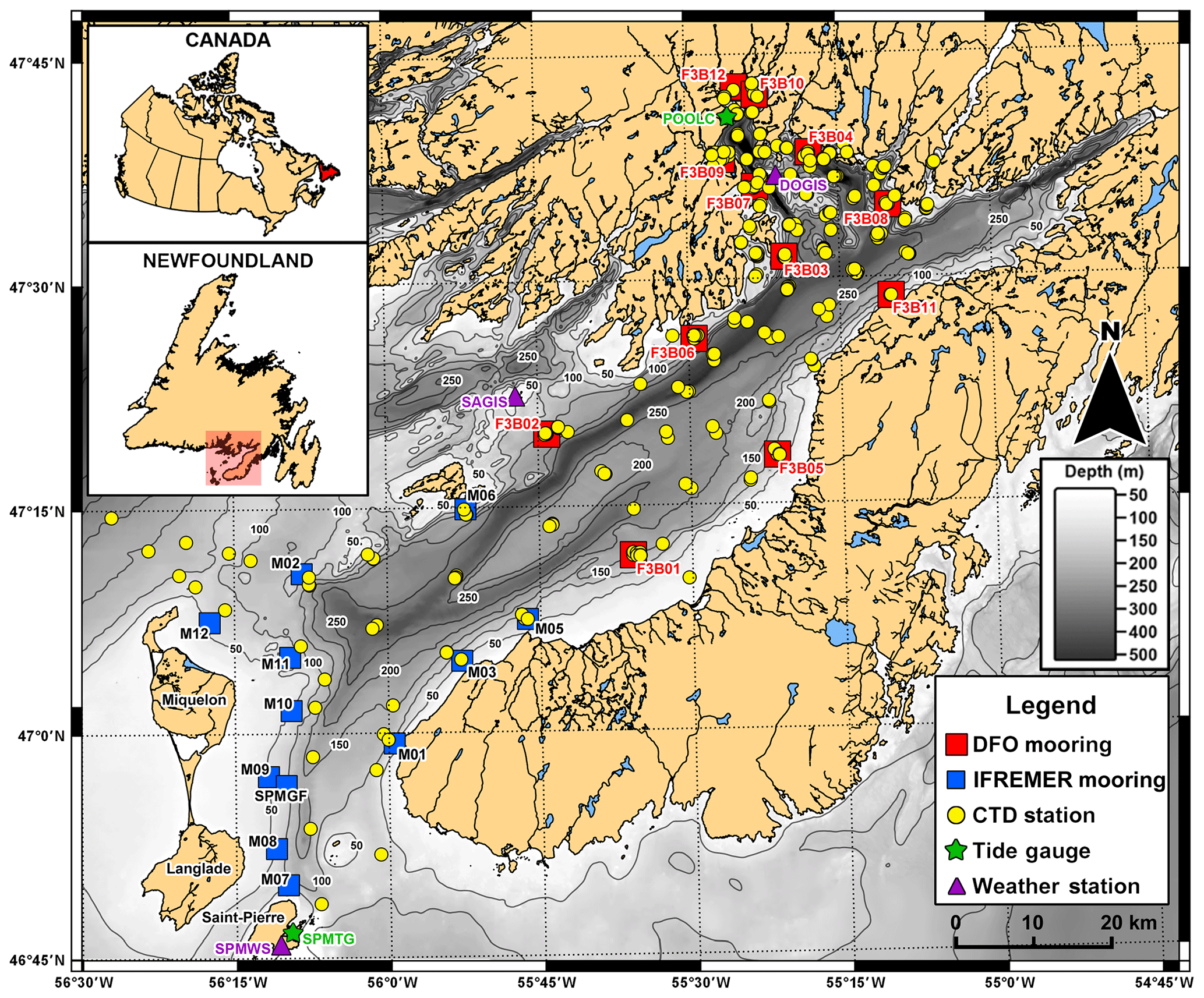
Figure 1Study area and summary of the observation program (May 2015–May 2017).
The observation program started in May 2015 with the deployment of eight moorings at four sites (F3B01-04), a weather station (DOGIS) and a tide gauge (POOLC). The program lasted for 2 full years (May 2015–May 2016 defined herein as “year 1” and May 2016–May 2017 defined herein as “year 2”) with maintenance trips occurring every 6 months. Thus, field operations occurred in May and November of each year for about 10–15 d each time, delimiting four observation periods defined herein as “legs”: May–November 2015 (leg 1), November 2015–May 2016 (leg 2), May–November 2016 (leg 3) and November 2016–May 2017 (leg 4). During each trip, additional measurements consisting of CTD (conductivity, temperature and depth) profiles were collected, and a separate trip was organized in August 2016 to get a better seasonal picture of the temperature and salinity field over the whole region. A small opportunistic survey, restricted to the Belle Bay area, also occurred in June 2016 during the re-deployment of mooring F3B08.
The moorings consisted of a string of thermistors mounted with a couple of CTD sensors (one within each main hydrographic layer) and one (year 2) or two (year 1) Acoustic Doppler Current Profilers (ADCPs) (Fig. 2). The setup changed from year 1 to year 2 by merging the originally separated ADCPs and thermistor–CTD sensor lines (by about 100–150 m), thereby doubling the number of main sites being monitored from four (F3B01-04) to eight (F3B01-08). Two other mooring lines were added, F3B09 and 10 and F3B11 and 12 for legs 3 and 4, respectively, to further increase the spatial resolution. With the exception of two moorings during leg 1 (F3B01 and 02), all moorings were of the subsurface, taut-line type. A surface spar buoy was used during leg 1 on F3B01 and 02 in an attempt to measure near-surface conditions and as a deterrent to fishing and shipping activities. The experiment was, however, unsuccessful with the loss of both surface buoys after about 5 months of deployment due to wave action wearing the mooring lines. Of those surface measurements, only one CTD dataset was partially recovered (RBR#60134 from F3B01, found on the shore with its spar buoy). Two main types of mooring were used during year 1 (Fig. 2), an “ADCP” type having a set of two upward-looking ADCPs separated by a string of thermistors and a “CTD” type consisting of two CTD sensors separated by a string of thermistors. The CTD type was declined in two versions for leg 1: surface (F3B01 and 02) and subsurface (F3B03 and 04). For leg 2, only the subsurface version was retained, adding a 9 m rope on the top part of F3B01 and 02. In year 2, the “CTD” mooring design of year 1 was used as a base and equipped with an ADCP on the bottom part (around 80 m) to combine water stratification with ocean current measures for most of the sites (F3B01-08). On F3B09 and 10, a simpler design was used due to the shallower depth of the sites and the need for less buoyancy and limitation on available hardware. To minimize drag we used 1∕4 in. Dyneema ropes and Open Seas SUBS buoys (Hamilton et al., 1997). CTD sensors were mounted in stainless-steal cages for protection, and thermistors were simply attached to the rope using cable ties and electrical tape. In most cases, acoustic releases were mounted in tandem for redundancy. Cooperation with our partner IFREMER (Institut Français de Recherche pour l'Exploitation de la MER) resulted in other sites being equipped with either bottom-mounted thermistors (M01–10 Mastodon, Lazure et al., 2015) or ADCP moorings (SPMGF) during some of the legs (leg 3 for M01–10 and all along for SPMGF).
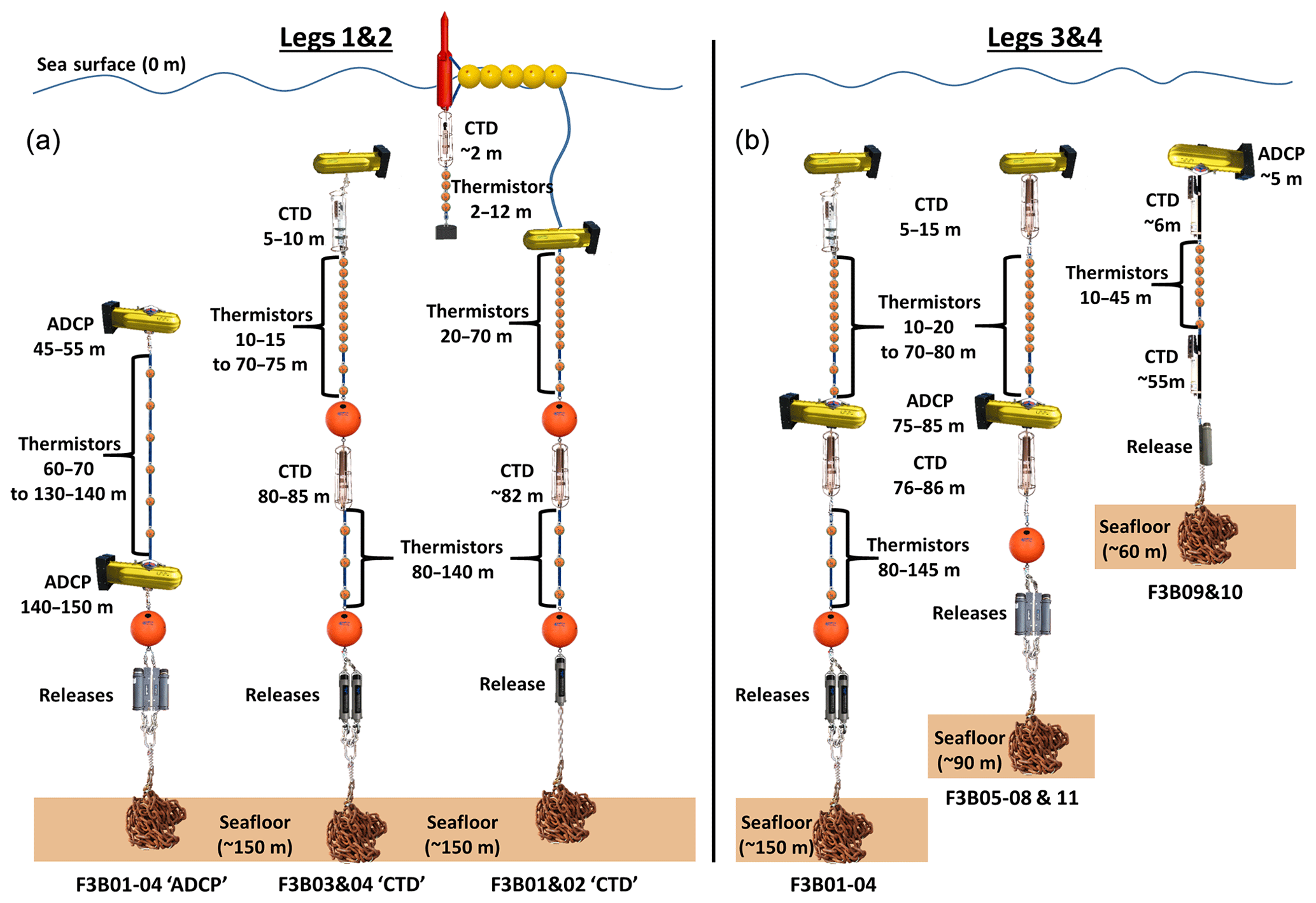
Figure 2DFO taut line moorings: legs 1 and 2 (a); legs 3 and 4 (b). In leg 2, F3B01 and F3B02 CTD lines were converted to the F3B03 and F3B04 design due to failures of the sea-surface part. A 110 m rope, without thermistors, was added under the bottom CTD of F3B08 to be deployed.
The other fixed (and long-term) structures were land-based and consisted of a weather station measuring wind speed and direction (at 2 and 10 m height above ground) as well as barometric pressure, air temperature, solar radiation (Qs) and photosynthetically active radiation (PAR) and of a tide gauge measuring the sea level and sea surface temperature. Two weather station structures were installed on a small, barren island (DOGIS; see Fig. 1 for location and Appendix A for an illustration): a 2 m height tripod on which was mounted a wind sensor, a barometer, a temperature sensor, a pyranometer (i.e solar radiation sensor) and a PAR sensor and a 10 m mast on which was mounted another wind sensor. The tide gauge was installed on a wooden wharf at the head of the bay (POOLC; see Fig. 1 for location and Appendix A for an illustration) and equipped with a vented pressure sensor mounted below chart datum in a black PVC tube to limit biofouling. These atmospheric and tide observations completed existing sites equipped by other agencies (Fig. 1): Sagona Island (SAGIS) weather station (Environment and Climate Change Canada), St Pierre airport weather station (Meteo France) SPMWS and St Pierre harbour tide gauge (Service hydrographique et océanographique de la Marine, France) SPMTG.
2.1 Instruments used
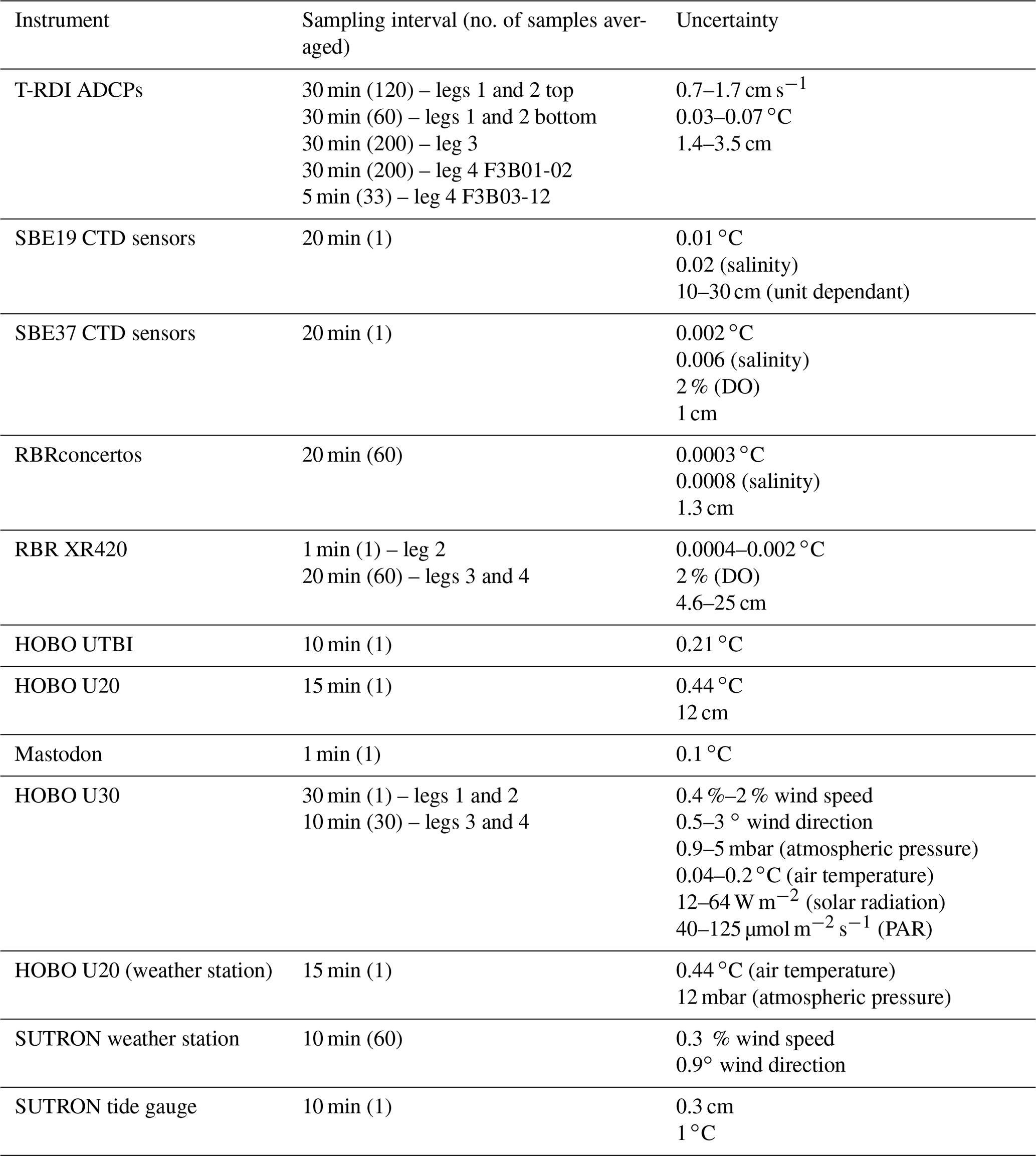
A variety of instruments was used during this program, selected for their proven and common use in the field of physical oceanography and atmospheric science. All our ADCPs were WorkHorse models (WH) from Teledyne RDI (T-RDI); most of them were of the 300 kHz type though a few 600 kHz and one 1200 kHz (WH300, WH600 and WH1200) types were also used during the second year. Most of the CTD sensors were Sea-Bird Electronic (SBE) instruments, model 19 (“SeaCAT” manufactured in the 1990s) with a few 37 models (“microCAT” manufactured in the 2000s). A few RBRconcerto CTD sensors as well as XR420 temperature–depth–dissolved oxygen instruments were used on some legs (typically as backup and/or complementary observations). All the thermistors used were disposable Onset HOBO TidbiTs (UTBI), and a few Onset HOBO U20 thermistors equipped with a pressure sensor were also used to complement the UTBI and provide additional depth information of the mooring line. Gill windsonic sensors were used on our weather stations to measure wind speed and direction and were plugged into an Onset HOBO U30 logger on the 2 m tripod and to a Sutron SatLink2 logger with real-time transmitting capability on the 10 m mast. An Onset smart barometric pressure sensor barometer (model S-BPA-CM10), an Onset 12-bit temperature smart sensor air temperature sensor (model S-TMB-M002), an Onset silicon pyranometer smart sensor (S-LIB-M003) and an Onset PAR smart sensor (S-LIA-M003) were also mounted on the 2 m tripod. A Sutron submersible pressure transducer (model 56-114) was used for the tide gauge, plugged into a Sutron SatLink2 logger with real-time transmitting capability. Characteristics and specifications of all the sensors used are provided in Table 1.
2.2 Instrument limitations and uncertainties
Due to their difference in memory and battery capacity, sampling strategy (i.e. interval) differed from one instrument to another. All the ADCPs were set to sample every 30 min during legs 1–3. For leg 4, a higher sampling rate of 5 min was chosen to increase temporal resolution on moorings F3B03-12. In year 1, ADCPs were set up in “burst mode”, that is sampling for a smaller amount of time than their sampling interval (7.5 min vs. 30 min) to avoid possible cross-talk interference since two instruments of the same frequency were used on the same line. In year 2, all the ADCPs were sampling evenly (i.e. continuously) along the sampling average period. Higher vertical resolution (1 m cell) and broadband mode were used during legs 1 and 2 for the near-surface units while lower vertical resolution (3 m cell) and narrowband mode were used for the near-bottom units to maximize range. Overall, a reduction of about 30 % in profile range from the manufacturer specifications was found due to the clarity of the water (i.e. low backscattering volume conditions). Based on first-year results, the sampling strategy was re-thought to increase the horizontal sampling in year 2 (eight or more sites vs. four) while keeping vertical profiling of the stratified part of the water column, i.e. from about 10 to 80 m depth. Cell size was increased from 2 m (leg 3) to 3 m (leg 4) to prevent loss of range during very clear water conditions usually observed in winter. Narrowband mode was used for all our units during year 2 for the same reason.
SBE and RBR CTD sensors were all set to sample at 20 min intervals while the XR420 instruments were set at 1 min intervals during leg 2 and 20 min during legs 3 and 4. The UTBIs were set to 10 min intervals along with the SUTRON weather station and tide gauge (with a 1 min internal average for the SUTRON). The U30 weather station was initially set up with a 30 min interval with no averaging during legs 1 and 2 and then adjusted to a 10 min interval, 30 samples averaged, during legs 3 and 4.
Table 1Instrumentation used, sampling setup and stated uncertainty (i.e. noise) based on manufacturer specification and sampling setup. “Top” and “bottom” refer to ADCP position on the mooring line during legs 1 and 2 (about 50 m vs. 145 m depth, respectively).
2.3 ADCP backscatter processing
To provide some added value, the ADCP backscatter data were processed to convert the raw returned signal strength indicator (RSSI, E in equation below), a measure of acoustic pressure received by the transducers, to a corrected backscatter volume Sv, proportional to the amount (i.e. volume) of particles present in the water column. The method used to do the correction is an updated version of the popular Deines method (Deines, 1999) published by Mullison (2017) and summarized by this equation (Mullison, 2017; Eq. 3):
Factory-calibrated values of Kc (count to decibel factor) and Er (noise floor) were used to solve this equation, along with the temperature measured at the transducer head by the instrument (Tx). Transducer temperature measured at transducer head and the salinity value selected during instrument setup (ES command; 32 in our deployments) were used to calculate the water absorption (a) along the range (from transducer) R, thereby implying homogeneous water conditions. The transmit pulse length LDBM was calculated using bin size (1–3 m) and beam angle (20∘) values. Default values of constant C and transmit power PDBW provided by Mullison (2017, Table 2) were used.
Overall, a combined uncertainty of 5 dB is estimated due to the assumption of water column homogeneity (constant absorption, 0.5 dB maximum error in summer toward the surface); the assumption of constant power source (±3 dB with alkaline batteries, decreasing in transmit power with time) affecting legs 1 and 2 ADCPs more than legs 3 and 4 ADCPs, which were using lithium batteries (featuring a quasi-constant transmit power all along a deployment), and inherent transducer linearity uncertainties (±1.5 dB according to Deines, 1999). This uncertainty is relatively small in comparison to the 55 dB average range (−90 to −35) observed along the program, i.e. less than 10 %, though not negligible. Note that this uncertainty can be qualified as being “relative” in a sense that it is an uncertainty applicable to any given time series taken separately. In absolute terms, bias can exist due to the assumption made on the constants C and PDBW, which may differ from one instrument to another.
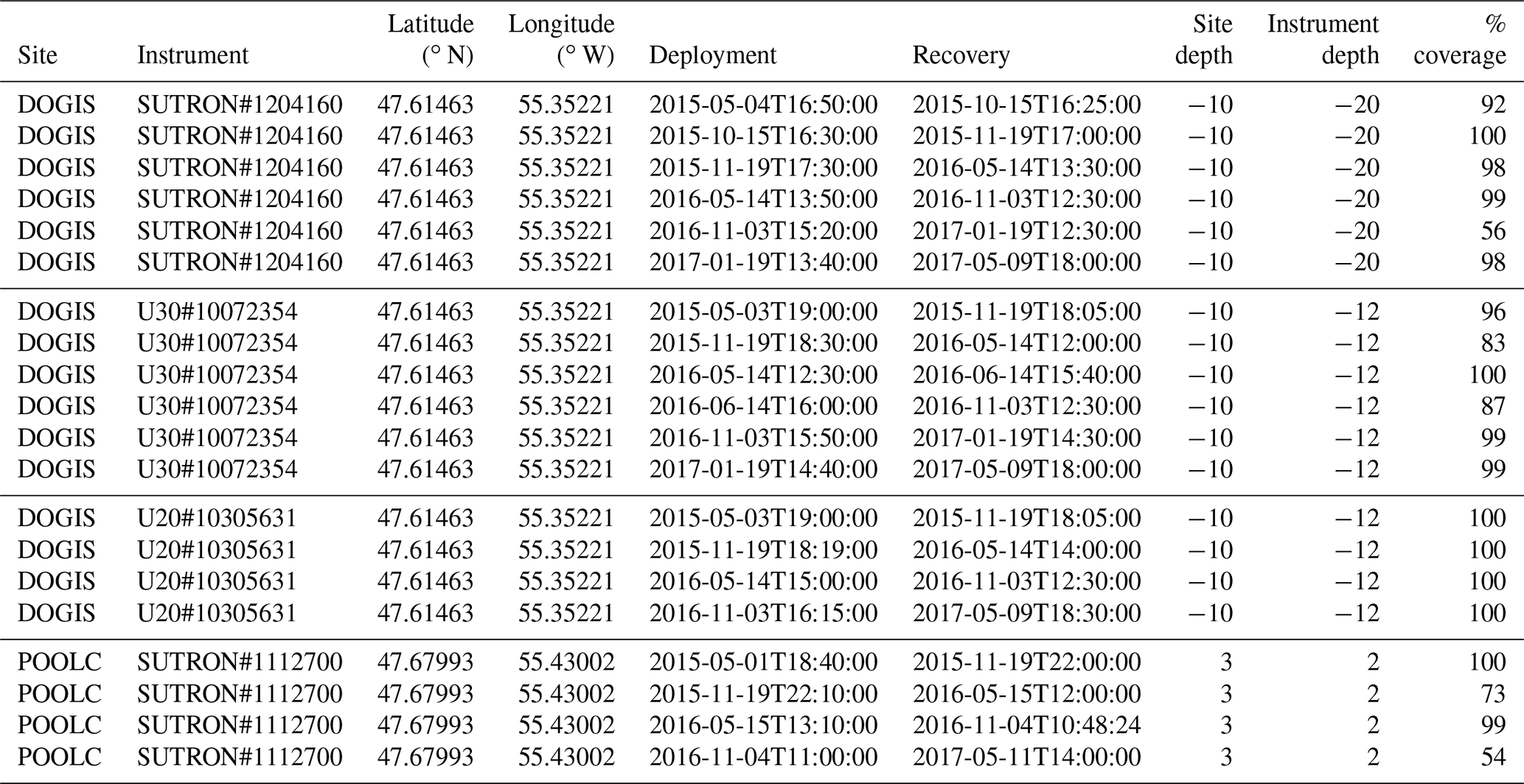
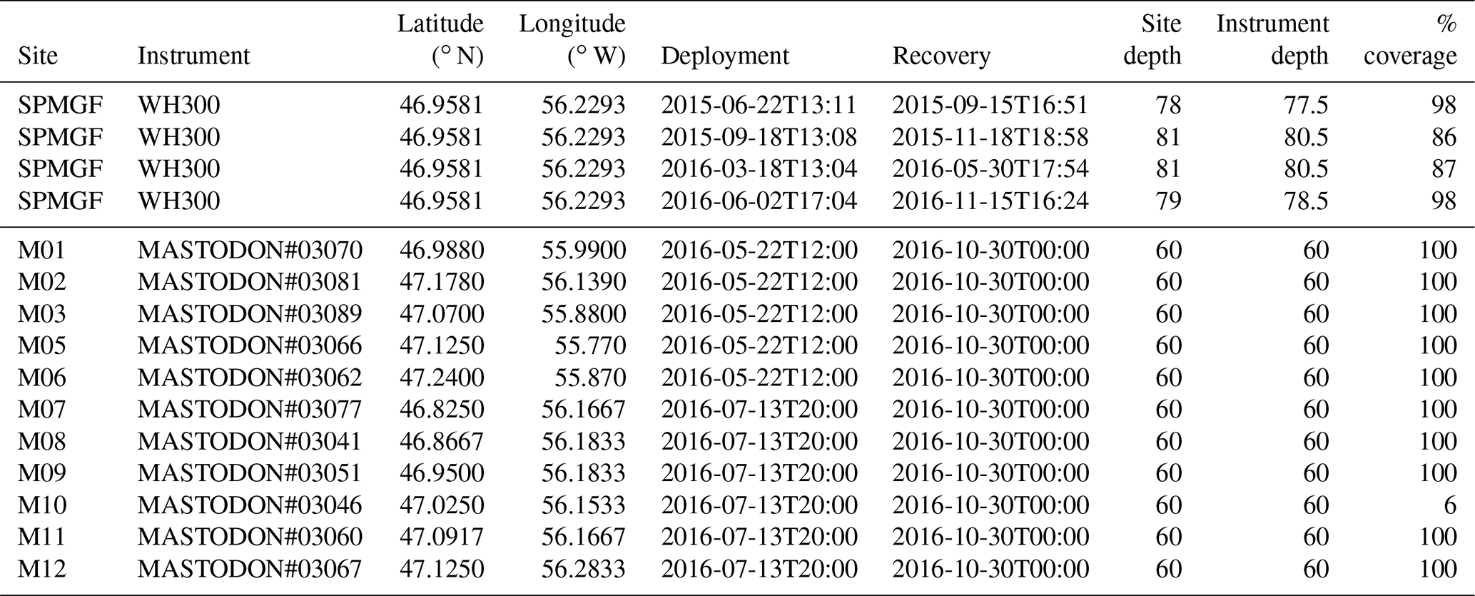
In total, 40 ADCP time series, 60 CTD/TD-DO time series (33 SBE19, 16 SBE37, 6 RBR XR420 and 5 RBRconcerto), 35 UTBI string series, 13 U20 time series, 11 Mastodon thermistor series, 16 weather station series (6 U30, 6 SUTRON and 4 U20) and 4 tide gauge series were collected (Appendix B, Tables B1–B6). Taken together, these time series amount to about 28 715 record days (about 79 years).
Percent coverage presented in Appendix B (Tables B1–B6) is calculated based on the recovered instruments and data only. Lost instruments or instruments from which no data could be recovered are not presented. In total one CTD was lost (RBR#60135 on F3B02, leg 1), one CTD sensor flooded without any possible data recovery (SBE19#1310 on F3B04 leg 2) and 14 UTBIs were lost (5 on F3B01-CTD leg 1, 5 on F3B02-CTD leg 1, 1 on F3B02-ADCP leg 2, 2 on F3B02-CTD legs 2 and 1 on F3B01 leg 3). Outside the failure of F3B01 and 02 top mooring part (10 units lost at once), UTBIs were typically lost during grappling operations when releases could not be triggered. There was also one failed deployment attempt at F3B08 during leg 3 (acoustic release failure in May 2016) which was successfully re-deployed in June 2016 but resulted in about 30 d of observation time lost (from early May to early June).
Percent coverages were calculated based on the good data recovery of current speed, current direction, current vertical speed and water column backscatter volume for the ADCPs; temperature, salinity and depth for the CTD sensors; temperature, dissolved oxygen and depth for the RBR TD-DO sensors; temperature and depth (or atmospheric pressure when used as a weather station sensor) for the U20s; temperature for the UTBIs; depth and temperature for the SUTRON tide gauge; wind speed and direction for the SUTRON weather station; and wind speed, wind direction, atmospheric pressure, air temperature, PAR and solar radiation for the U30 weather station. For each instrument, the percent coverage represents the useable data covering the expected periods of observation; for a multiple-parameter instrument (as listed above) the percent coverage was calculated for each parameter and then averaged per instrument.
Overall, the coverage is about 93 % without considering instrument losses and about 91 % when considering the losses. Illustrations of the data coverage are given in Figs. 3 and 4 as Gantt charts.
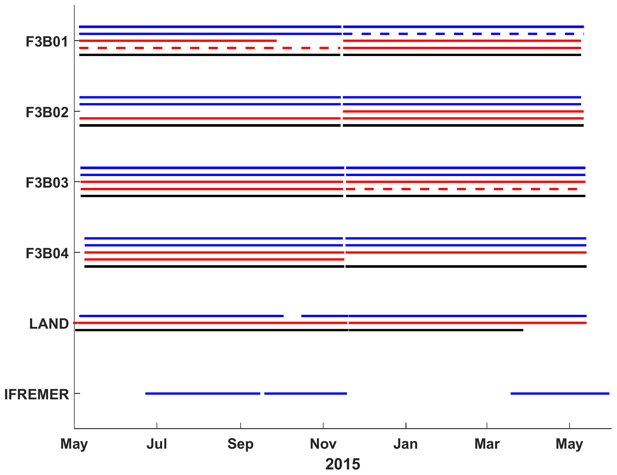
Figure 3Data return, legs 1 and 2. For the moorings F3B01-04, ADCPs are in blue, CTD sensors are in red and UBTIs are in black. The top lines correspond to the shallowest unit. For the land-based stations (LAND), DOGIS SUTRON weather station are in blue, DOGIS U30 weather station is in red and POOLC SUTRON tide gauge is in black. IFREMER ADCP data (SPMGF) is in blue. Dashed lines represent partial data recovery (e.g. ADCP tilted, CTD having no or partial salinity return).

Figure 4Data return legs 3 and 4. For the moorings F3B01-12, ADCPs are in blue, CTD sensors are in red and UBTIs are in black. The top lines correspond to the shallowest unit. For the land-based stations (LAND), DOGIS SUTRON weather station is in blue, DOGIS U30 weather station is in red and POOLC SUTRON tide gauge is in black. IFREMER ADCP (SPMGF) and MASTODON (M01-12) data are in blue and black, respectively. Dashed lines represent partial data recovery (e.g. ADCP tilted, CTD having no or partial salinity return).
The primary objective of this observation program was to collect a robust baseline for studying the main physical processes affecting Fortune Bay. In particular, upwelling and downwelling propagations associated with strong currents along the shoreline were thought to be important features based on previous work done locally (Salcedo-Castro and Ratsimandresy, 2013; Donnet et al., 2018a) and in other embayments of the region (Yao, 1986; de Young et al., 1993; Davidson et al., 2001; Ma et al., 2012). Hence, Fortune Bay's strong seasonal stratification, steep slopes, weak tides, strong along-shore winds and large width all indicated a potential for such “coastally trapped” processes to occur.
The observation program was therefore designed to measure water vertical stratification and currents as well as forcing (i.e. wind and sea level) over timescales of tens of minutes to a year and taken at as many locations as possible along the coast, within one internal Rossby radius, to follow potential disturbances travelling around the bay. Such features were indeed observed, and an example of them is presented in Fig. 5. The study of those features, including their generation, propagation, scale and importance for particle advection and water renewal, key aspects in studying the effect of aquaculture on the environment, will be the focus of future publications.
The uncertainty estimates presented in Table 1 are based on the instrument specifications and sampling strategy. That is, they represent the expected short-term (i.e. noise) fluctuation around the true measure and assume a perfectly calibrated instrument, i.e. no bias. Laboratory testing and in situ performance checks was performed to further assess these estimates and correct for eventual bias. Laboratory testing were performed in a 3 m depth seawater tank (for the CTD sensors, mainly) to check temperature, salinity and depth measurements, and a stable temperature water bath was used to check temperature measurements (for the UTBI, mainly). In situ checks were obtained using CTD casts taken just after deployment and right before recovery of the moorings and by cross-checking/comparing each instrument from the same mooring line (e.g. pressure measurements). The main biases found were with the pressure sensors of the moored Sea-Bird Electronic model 19 (SBE19) instruments, which could be as large as 6 dbar (∼ 6 m of water depth). A combination of tank test results and in situ checks using the ADCP (and other instruments when available) and mooring line length were used to determine these pressure biases. Both pressure sensor data and corrected backscatter data (i.e. converted to volumetric backscatter values Sv in decibels) were used to determine the in situ depth of the ADCP (i.e. the distance to water surface when using backscatter values), which was then used to crosscheck the depth of the CTD sensors along the line. Biases that could not be determined with reasonable certainty resulted in discarding the data. Except for leg 1, each moored CTD was sent to the manufacturer for calibration prior to deployment. For leg 1, only laboratory tests could be done. All the thermistors used were new, i.e. bought for this program, and the ADCPs were 3–7 years old. The CTD profilers used were sent to the manufacturer for calibration on a yearly basis with a 3-year rotation scheme; i.e. three CTD profilers were available for this program and one profiler was sent per year to be used as a reference for the other two in laboratory and in situ calibration/performance checks. Overall, it is estimated that the absolute depth of each instrument is known to the nearest metre, that the temperature is accurate at ±0.2 ∘C (UTBIs) or less (CTD sensors), that the salinity is within 0.1 (moored CTD) or less (CTD profiles) from the true value and that the current speed accuracy is ±2 cm s−1 or better. Note that if further averaging were to be done on those original time series, the uncertainty would go down by the square root of the number of samples taken per sampling average except for the ±1 m uncertainties on depth which can be seen as an unknown bias.
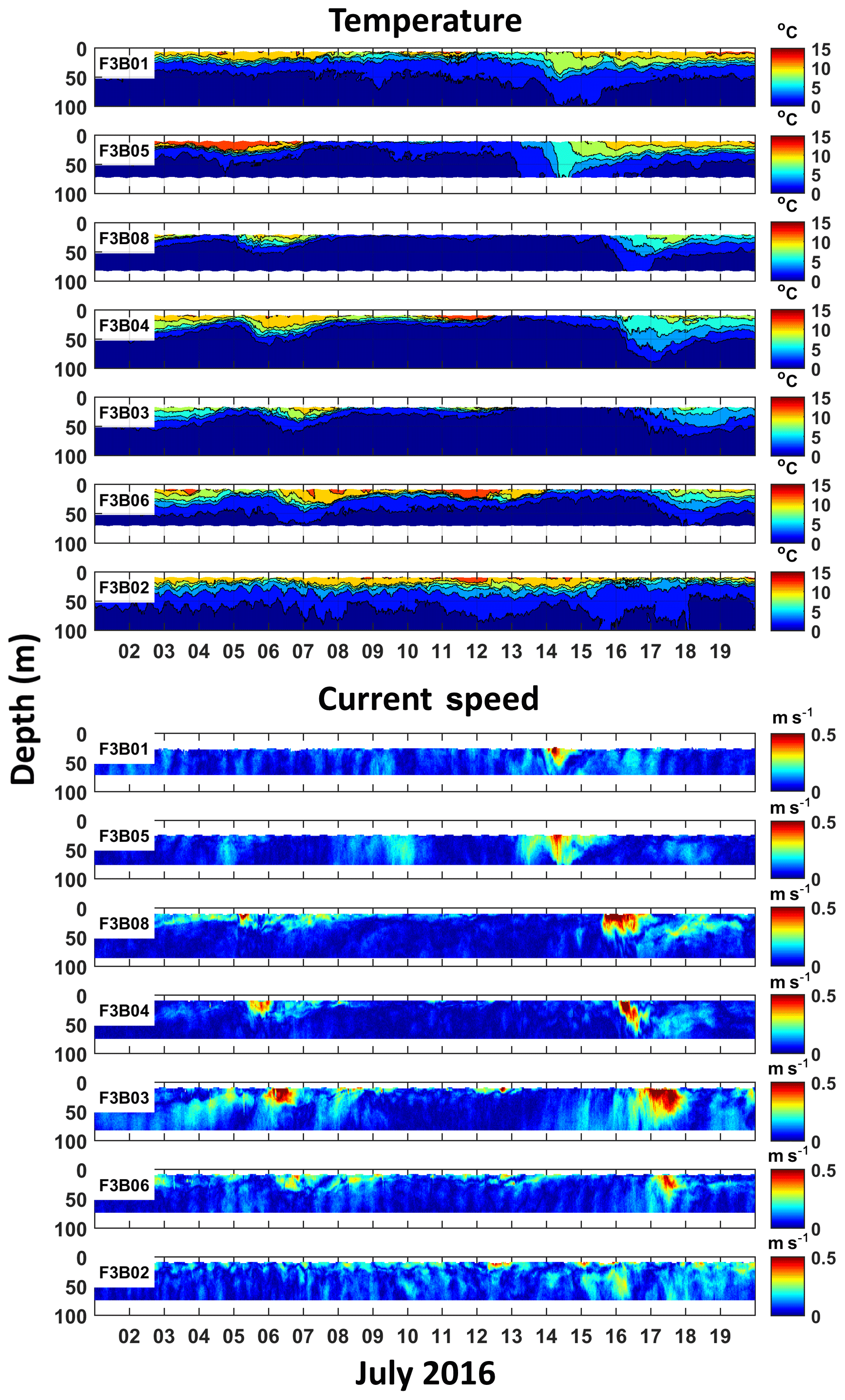
Figure 5Fortune Bay water column thermal stratification and currents from 1 to 20 July 2016 showing several upwelling and downwelling events associated with strong current “pulses” travelling around the bay, i.e. from moorings F3B01 to F3B06.
4.1 Data limitations and issues
The program suffered from some instrument failures. ADCPs from F3B09 and 10 during leg 3 suffered from a battery failure (F3B09) and from a memory card failure (F3B10), resulting in data coverage of only 48 % (slightly less than 3 months) and 17 % (about 1 month), respectively. Two SBE19 CTDs (no. 1310 and no. 1312) got their electronic casing flooded, resulting in a complete loss of data on F3B04, leg 2 (SBE19#1310) and in partial losses (small leak) on F3B03, leg 2, and on F3B07, legs 3 and 4 (SBE#1312, temperature and salinity data corrupted). The DOGIS SUTRON weather station suffered from a solar panel failure during leg 1, resulting in a reduced coverage of 92 % (a loss of about 12 d) and from a wind sensor failure during leg 3 (56 % coverage, a loss of about 33 d). DOGIS U30 weather station suffered from barometer issues during legs 1, 2 and 3, reducing coverages to 96 %, 83 % and 87 %. The POOLC tide gauge also suffered from sensor failures, during both leg 2 and leg 4 of the program, resulting in reduced coverages of 73 % (47 d lost) and 54 % (86 d lost) and no coverage during the late winter–early spring seasons.
The program also suffered from some human errors and practical difficulties. Notably, tangling of mooring ropes has resulted in excessive vertical tilt orientation of the upward-looking ADCP on moorings F3B01, 05 and 07 of leg 3 and on F3B05 of leg 4, corrupting the data (see details below). In the case of leg 3 (F3B01, 05 and 07), problematic deployments in which the mooring line was not properly kept tight prior to releasing the anchor likely played a role. In the case of leg 4 (F3B05) it is less obvious since a stricter mooring deployment procedure was then in place, and those fieldwork records do not indicate any wrongdoing. The use of SUBS buoys, though improving mooring drag and potential “knock-down” from strong currents, increases deployment difficulty when they are placed in the middle of a mooring line (as opposed to the top of a line) since they have a natural tendency of orienting themselves in the flow and thus to have the rope close to their back fin when sinking downward, thereby increasing the chances of being tangled. It should be noted that one case of tangling/excessive ADCP vertical tilt occurred to the bottom ADCP of F3B01 during leg 2, after about 3 weeks of deployment (see below for details and Fig. 7), thus not likely due to a deployment issue. Fishing activities may have caused it, though no evidence of it could be found by looking at the data (e.g. rise and fall of the mooring). The data sampling frequency of the ADCP (30 min) prevents a fine examination, though no obvious evidence of mooring movement could be seen with the higher-frequency UBTI records either (10 min), and fishing activities during that time of the year (December) are not very likely. The issue occurred during a strong current event, indicating that strong current shear could potentially be an actor.
4.2 QA/QC and data processing methods
Data were processed and quality checked similarly for all the instruments as follows.
-
Raw data were first converted to the most convenient format known/available to the authors.
-
Time stamp and all variables of interest were extracted from the raw data, and meta-data were associated with the dataset (i.e. station ID, geographical coordinates, deployment and recovery date and time, and instrumentation ID).
-
Using deployment and recovery time, “out-of-water” data were removed.
-
Clock drift and depth offset were assessed and corrected using concurrent data available on the same line. ADCPs were most often used as a reference since their pressure sensors were systematically “zeroed” prior to deployment, and their clock did not drift more than a few minutes per deployment. U20s and RBRs were usually used as a secondary reference or as a primary one when no ADCPs were available on the same line (e.g. in legs 1 and 2). SBE19 units were the most affected by clock drift and depth offset. A few units (SBE19 as well as UTBI) were also found to have been set up in local time instead of UTC, mistakenly.
-
“Out-of-range” data were removed using automatic filters following the criteria shown in Table 2. ADCP criteria were largely based on the manufacturer recommendations with current speed less than 0 (bad values are actually logged as −32 768; see T-RDI documentation no. P/N 957-6156-00, p. 147), percent good (PG) less than 25 (T-RDI documentation no. P/N 957-6156-00, p. 150) and instrument tilt over 15∘ from the vertical (T-RDI documentation no. P/N 957-6150-00, p. 17) used to remove bad data. Instrument vertical tilt was calculated using the pitch and roll records (see below for details). In addition to those data quality filters, a “surface rejection” filter was applied as a percentage of the range to sea surface (or sea bottom for the downward-looking F3B09 and 10) usually equal to 10 % (i.e. a little higher than the theoretical 6 % stated for 20∘ beam angle ADCPs, T-RDI documentation no. P/N 951-6069-00 p. 38). Trial and error was performed for this latter filter by examining the velocity, backscatter and correlation profiles of each of the time series. In the case of severely tilted instruments (details below) up to 30 % of the range needed to be removed. Speed, PG and surface rejection filters were applied to all the velocity and backscatter data while tilt filter was only applied to the current velocity direction and “earth”, components of the velocity data (i.e. eastward u, northward v and vertical w; details in technical validation section). For the other instruments, out-of-range filters were based on the expected ranges, i.e. values that would be realistically impossible to attain within the study area, and/or based on default values given automatically to bad data by the logger (e.g. PAR and Qs<0; see Table 2 for details).
-
A manual “despiking” was finally performed by plotting the data and examining the time series visually. Minimal rejection was done to avoid rejecting potential “outlier events”. As a result, some spurious data points may still be present in some time series.
The CTD profiles were processed using SBE data analysis software, and recommended procedure as described in Donnet et al. (2018a). CTD profiles were averaged in 1 m bins and visually checked individually.
Table 2“Out-of-range” filters used to quality control the data.

4.3 UTBI depth calculation
Since our thermistors (UTBI) did not have embedded pressure sensors, the depth of their temperature records needed to be estimated. This calculation was done in three steps, increasing the accuracy of the estimate at each step.
-
Once a site depth was accurately determined, mean depth of each UTBI was determined using the mooring diagrams providing with the distance from sea bottom of each instrument. Mean depth (with respect to mean sea level, MSL) was then determined as site depth minus height above sea bottom.
-
“Tidal depth”, i.e. depth varying due to the tide alone, was determined using the results of tidal analyses made on the instruments equipped with a pressure sensor (i.e. ADCP, CTD and U20). One reference per mooring line was used, typically the instrument located the closest to the top of the mooring having the highest data coverage so that the overall mooring tilt was best approximated (CTD or U20). Tidal analysis was done using the T_TIDE programs (Pawlowicz et al., 2002), and UTBI “tidal depths” were calculated as MSL depth plus tide.
-
Finally, to take the mooring movement into account, i.e. lateral movements of the mooring line due to current drag, an “absolute depth” was determined using an estimate of the mooring horizontal tilt angle. Tilt angle was determined using the same depth time series from which a tidal analysis was performed for the previous step. A water level residual was then calculated as measured water level (from MSL) minus tide. This residual was then used to calculate a mooring line tilt angle series as tilt , where H is the instrument height above sea bottom at any given time and L is the instrument height at rest (i.e. its mean height). Using the horizontal tilt angle time series, UTBI series of height above sea bottom were calculated as , where L is the UTBI height above sea bottom at rest. The “absolute depth” series was then determined as site depth minus H plus tide.
Overall, the mooring lines' average vertical tilt was below 5∘ (2–4∘ with a standard deviation of the order of 1–2∘) with maximums on the order of 15–25∘ during extreme events, corresponding to vertical mooring displacements of about 5–15 m. These vertical “knock-downs” are large compared to the 1–2 m tidal range reported in the region (Donnet et al., 2018b) but relatively small in comparison to the mooring line length (about 5 %–10 %), indicating good mooring performances.
It should be noted that these estimates of tilt and therefore instrument depths assume no other external variation in sea level than the tides. Other factors such as storm surges or shelf waves can affect the sea level on the order of 0.2–1 m in the region (e.g. Tang et al., 1998; Thiebaut and Vennel, 2010; Han et al., 2012; Ma et al., 2015). A preliminary inspection of our tide gauge records (not shown) indicate that residuals, i.e. water level variations not attributed to tides, of the same range were observed during our program.
4.4 In situ comparisons (e.g. CTD profile vs. mooring data)
A CTD cast was performed after each mooring deployment and just before mooring recovery (see Fig. 6 as an example). Thus, a total of 52 casts were available for in situ checks (F3B03 and F3B04 pre-recovery casts were missed). The primary goal of those checks was to assess the performance of the moored UTBI lines (temperature) and moored CTDs (salinity).
Overall, a mean difference of 0.12 ∘C and associated mean standard deviation of 0.11 ∘C were found between the CTD profiles and UBTI observations, and an overall mean salinity difference of 0.07 and mean standard deviation of 0.03 between the CTD profiles and moored CTD sensor were obtained.
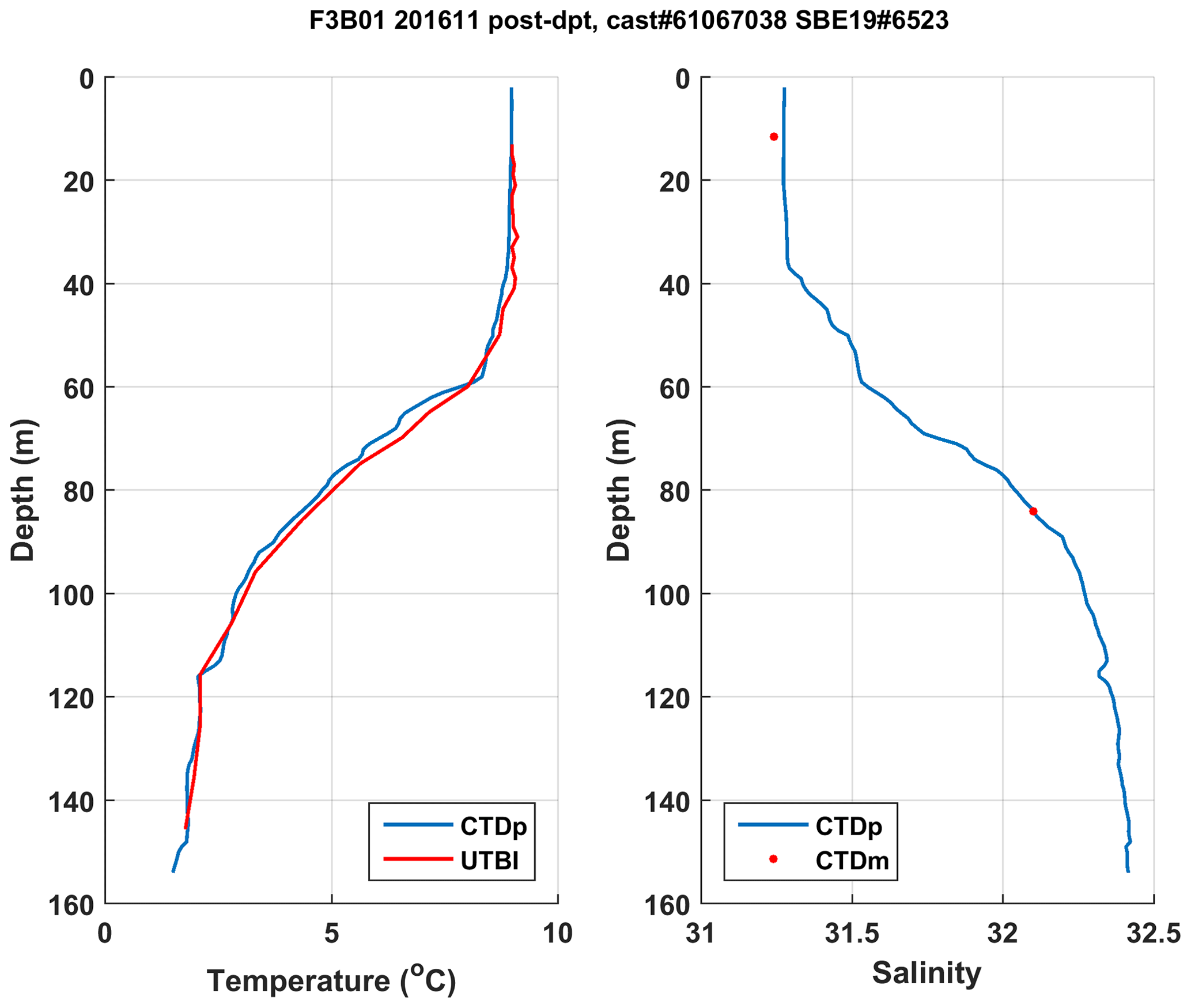
Figure 6In situ CTD profile (CTDp) comparison with moored thermistors (UTBI) and moored CTD (CTDm) on 7 November 2016 at F3B01.
4.5 ADCP tilt issue
Excessive vertical tilt affects ADCPs' gyrocompass by biasing the heading, which corrupts trigonometric rotation from instrument coordinates to earth coordinates (T-RDI, personal communication, 2018, 2020, and details in T-RDI documentation no. P/N 951-6079-00). T-RDI indicates that while their attitude sensor can measure tilts (i.e. pitch and roll) up to about 20∘, tilts above 15∘ will irreversibly corrupt the data (T-RDI documentation no. P/N 957-6150-00 p. 17). If the tilt, however, stays within a measurable range (i.e. 15∘ to about 20∘), bin mapping will still hold (T-RDI, personal communication, 2018; see details in T-RDI documentation no. P/N 951-6079-00), and, thus, horizontal measurements of current speed and backscatter, i.e. variables not affected by erroneous heading, will still be correct and properly “mapped”. At 20∘, any given beam may end up being oriented horizontally, which prevents the derivation of the horizontal component of the current. A three-beam solution may still work but the flow horizontal homogeneity assumption cannot be assessed (the so-called “error velocity”; see T-RDI documentation no. P/N 951-6069-00 p. 14 and P/N 957-6150-00 p. 14 for details), thereby limiting quality control. Beyond the tilt sensor limits (i.e. in pitch and roll axes) which can be anywhere from 20 to about 25∘ (see Table 3), current speed calculation and bin mapping will become biased; profile data will then likely be unrecoverable. An illustration of this issue and potential recoverable data is presented in Fig. 7. The top 50 m (not affected by over-tilted position) and bottom (over-tilted from 7 December) ADCP profiles are plotted together, showing the effects of the tilt on current direction and current vertical component w but not on current speed and acoustic backscatter.
In our quality control process, a “combined” tilt angle, i.e. combination of pitch and roll angles, was used to filter unreliable current direction and earth coordinate velocities (i.e. u, v and w). This combined tilt was calculated as follows:
This rejection is somehow conservative since this combined angle is always larger than the pitch and roll taken individually.
In addition to this automatic filter, bench tests were performed on each of our ADCPs to determine their maximum pitch and roll angles measurable by placing each unit horizontally on a table on each direction, i.e. beam 1–2 and beam 3–4 axes, which helped us to further assess the quality of our data (Table 3).
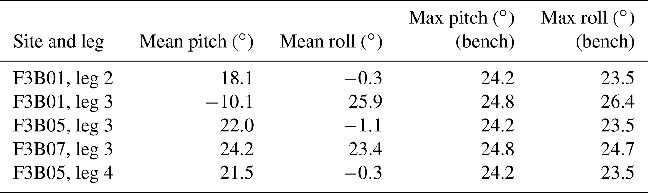
Five time series were affected by this issue in total: F3B01 leg 2 (bottom unit), F3B01 leg 3, F3B05 legs 3 and 4, and F3B07 leg 3. Being tilted near both pitch and roll limits, the latter was corrupted beyond repair, and nothing could be saved from it. The other four were generally severely tilted, but below the limits and on one side “only”; current speed and backscatter profiles were saved from those time series.
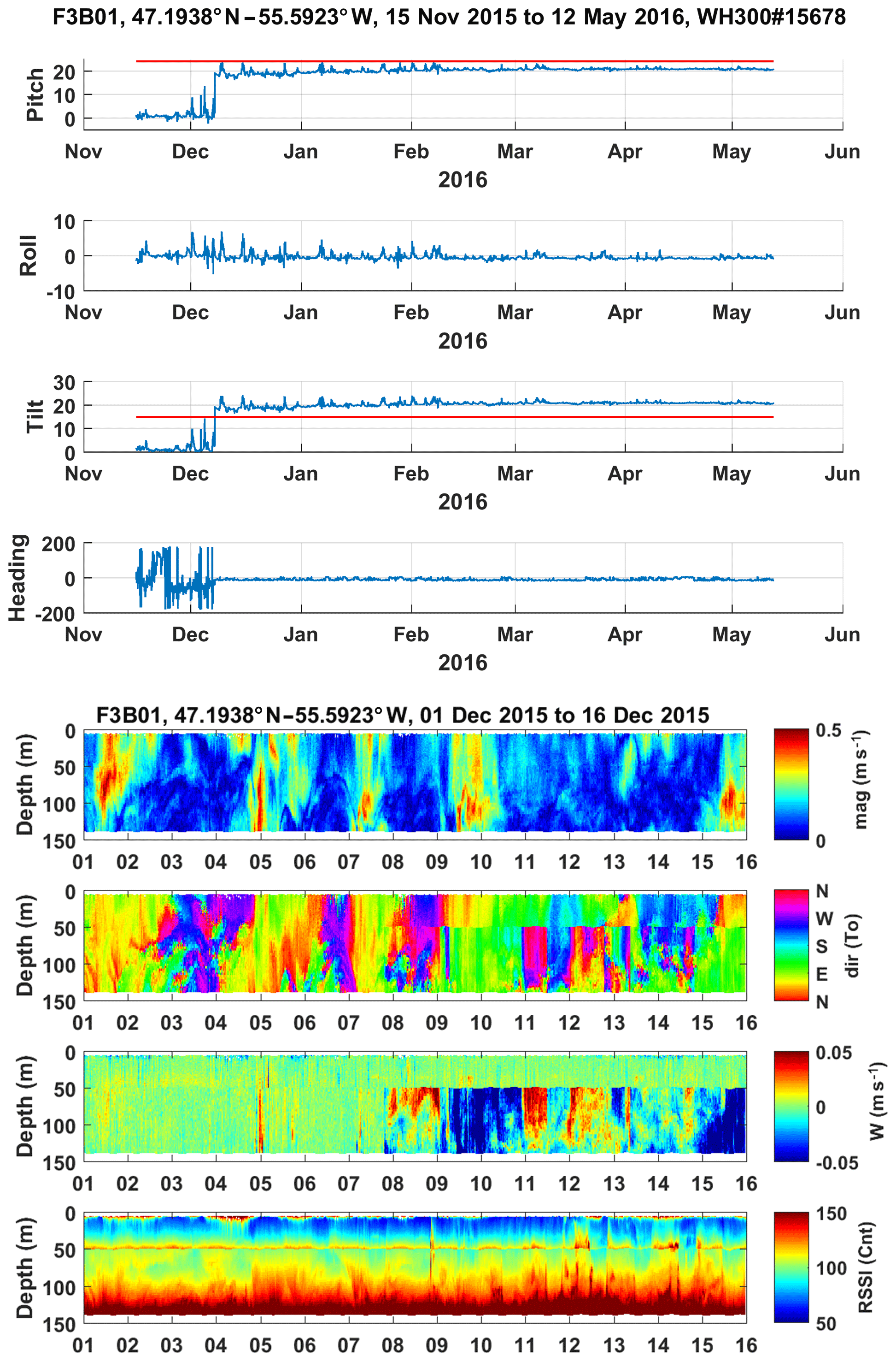
Figure 7Example of an ADCP over-tilted issue. The event occurred on 7 December 2015 between 18:30 and 19:30 UTC, tilting the bottom ADCP of the mooring line on the pitch axis. The top four panels show the attitude sensor, pitch (first panel), roll (second panel), calculated “combined” tilt angle (third panel) and heading (fourth panel and as recorded by the instrument). Red lines on the pitch and tilt plots indicate the maximum sensor range as determined by bench test and the maximum accepted tilt angle of our quality control filter. The bottom four panels show current speed (mag), current direction (dir), current vertical component (w) and raw backscatter data (RSSI) zooming on the period 1–16 December 2015.
Processed data are available from the SEANOE repository (https://doi.org/10.17882/62314, Donnet and Lazure, 2020). One file per time series was created in the NetCDF format containing a header with key metadata (site ID, geographic coordinates, site depth, instrument used, author and date of creation) and the data themselves with consistent variable naming (e.g. time, depth, temperature etc.). UTBI time series were bundled together into one folder per mooring line and, thus, one processed file per time series. CTD profiles were bundled up per survey and formatted as tab-delimited ASCII ODV4 files (Schlitzer, 2019). NetCDF files were created under the MATLAB environment and tested using the NetCDF utilities (ncdump from unidata), Python (with xarray and panda libraries) and the Interactive Data Language (IDL) environments. Care was taken to export as much data from the raw as possible (e.g. ADCP correlation magnitudes), but they are provided as “processed”; that is, bad data flagged by the QA/QC (quality assessment/quality control) process described below were replaced by NaN (not a number) values.
We present an oceanographic dataset collected in a subpolar, mid-latitude, broad fjord. The data collection was centered on the deployment and recovery of oceanographic moorings and a few land-based stations collecting physical parameters such as water temperature and salinity, ocean currents, wind speed and direction, and tide. The main goal of this observation program was to serve as a base to further study the main physical processes affecting this embayment which are likely common to other wide stratified fjords. To our knowledge, very few embayments alike, i.e. broad fjords, have such comprehensive observations combining numerous and continuous in situ sampling points. Several bays in the region have been well explored in the past but their continuous observation via moorings rarely extended more than a few months during the spring to fall seasons, thus not offering a complete seasonal picture (e.g. Yao, 1986; de Young and Sanderson, 1995; Hart et al., 1999; Schillinger et al., 2000; Tittensor et al., 2002a, b). Abroad, with the increasing interest in polar regions and their importance in climate, many recent studies relied on significant datasets collected in broad fjords (e.g. Straneo et al., 2010; Jackson et al., 2014; Inall et al., 2015; Merrifield et al., 2018). Generally, and most likely due to extremely challenging technical constraints (e.g. massive glacial ice), those datasets remain scarce and limited to a few points and/or few months of observation, however. A notable exception to this scarcity is the important research effort spent in Svalbard since 2002 (see Hop et al., 2019, for a review).
By combining a relatively large number of observation points (up to 21 moorings during leg 3), high vertical resolution in both thermal stratification (2–10 m) and ocean currents (1–3 m), and duration (2 years), we believe that this dataset should be comprehensive enough to study a wide variety of processes, making it of particular interest to be shared.
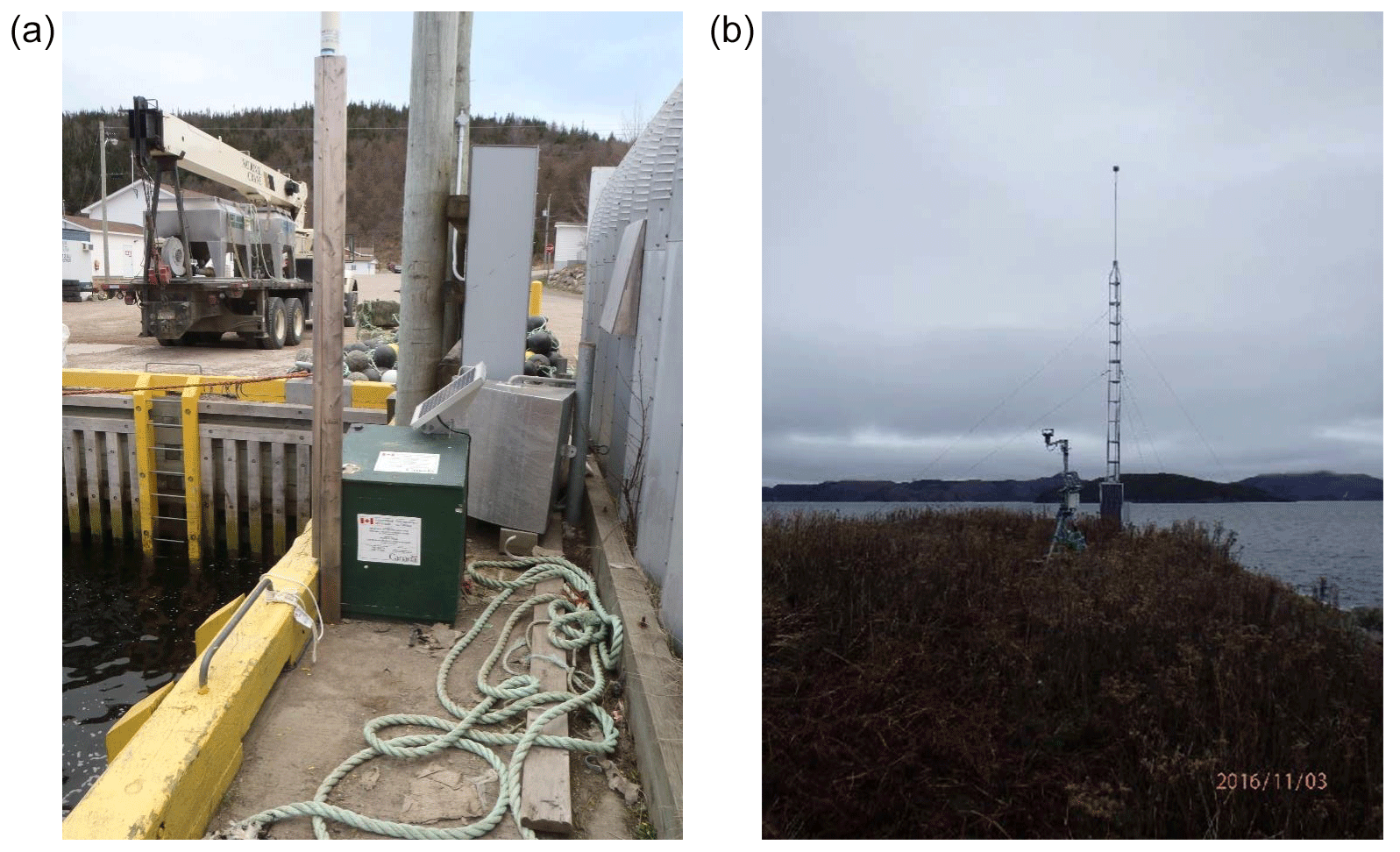
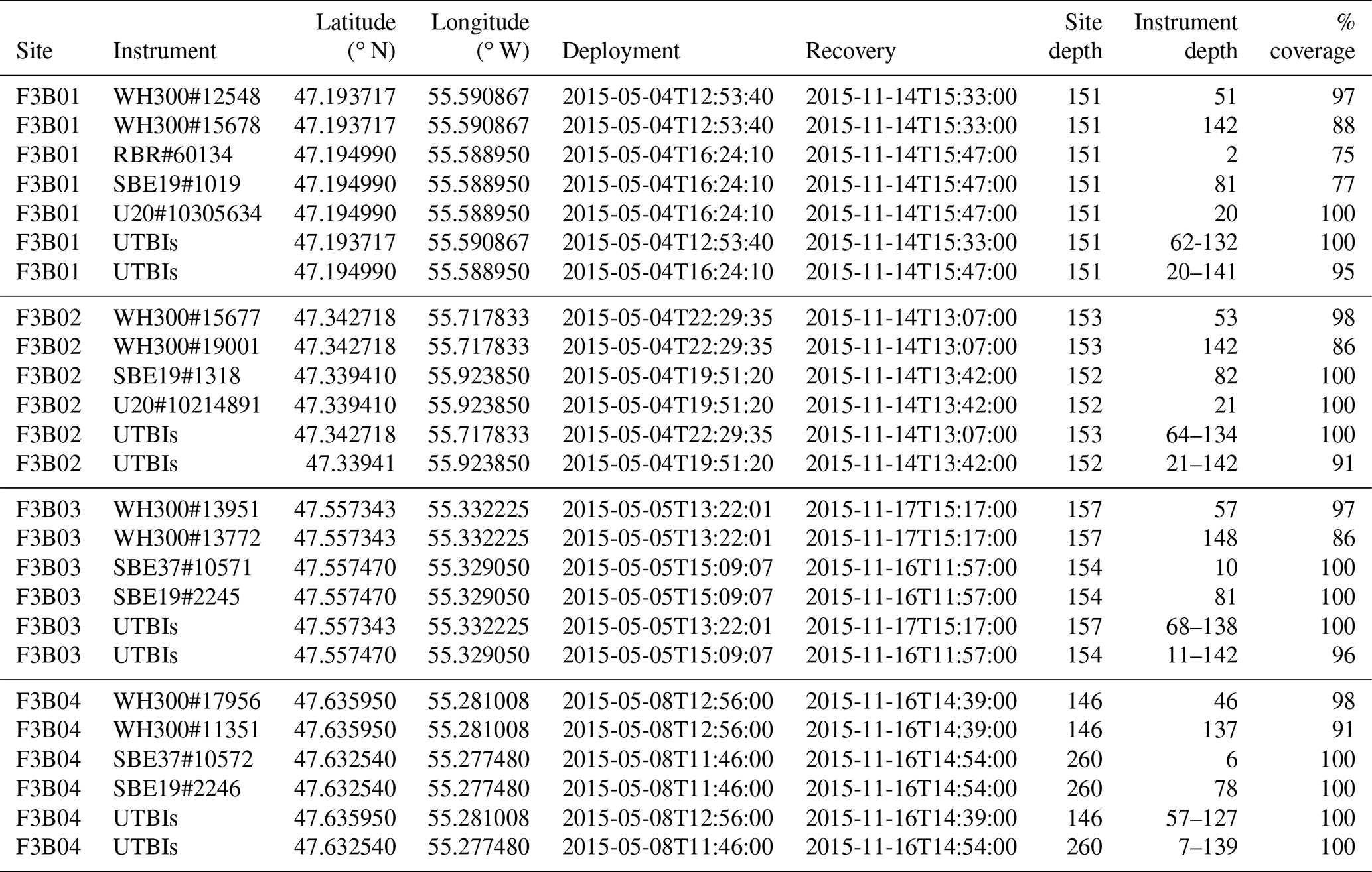
Table B2Data collection summary, leg 2 (November 2015–May 2016).
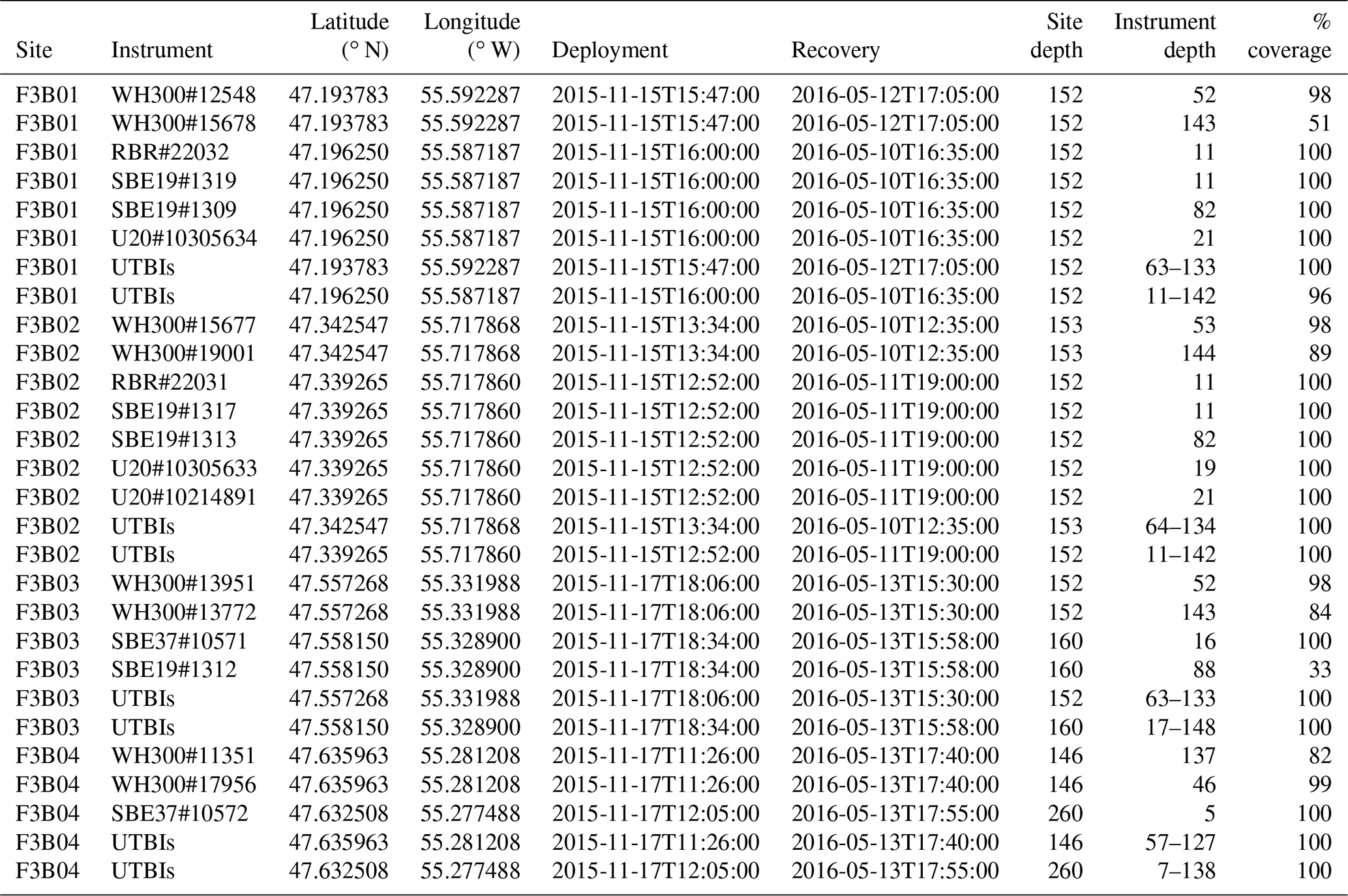
Table B3Data collection summary, leg 3 (May 2016–November 2016).
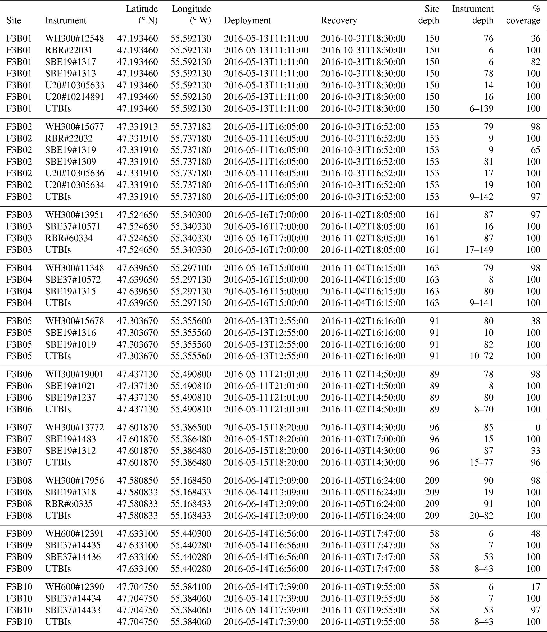
Table B4Mooring data collection summary, leg 4 (November 2016–May 2017).
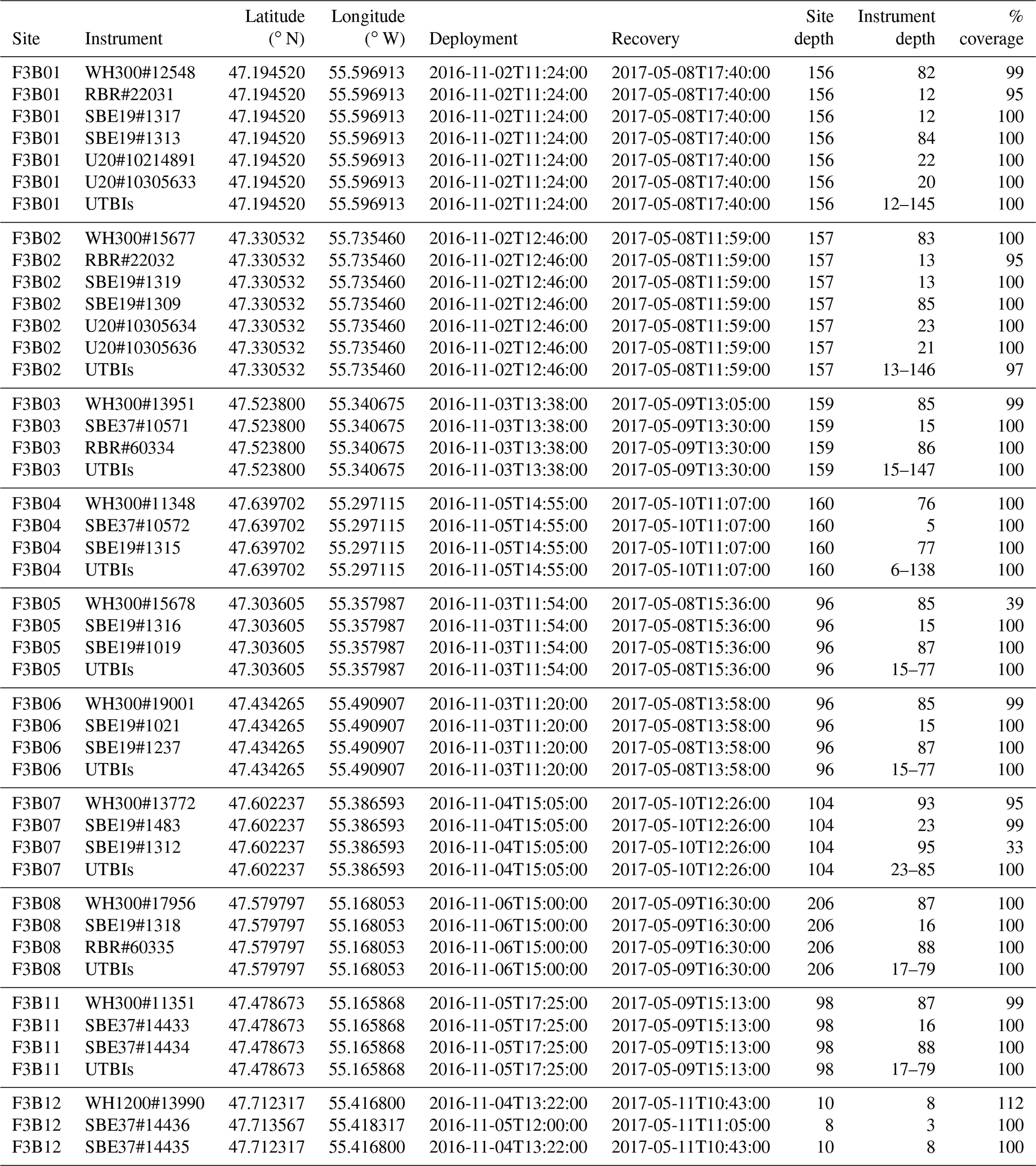
Table B5Land-based data collection summary for the whole program (May 2015–May 2017).
SD designed the study with the assistance of PL, AWR and GH. SD designed and directed the fieldwork, including the mooring design and pre-implementation modelling. SD processed all the data except those from the Mastodon, which were processed by PL. SD designed and led the QA/QC procedures and data analyses with contributions from PL, AWR and GH. SD prepared the figures and wrote the manuscript with contributing reviews from PL, AWR and GH.
The authors declare that they have no conflict of interest.
The data are published without any warranty, express or implied. The user assumes all risks arising from their use of the data. The data are intended to be research quality. It is the sole responsibility of the user to assess if the data are appropriate for their use and to interpret the data, data quality and data accuracy accordingly. Authors welcome users to ask questions and report problems.
A number of people contributed to the field effort and to them we are very grateful; many thanks to Dwight Drover (DFO legs 2–4), Pierre Goulet (DFO legs 1 and 2), Kim Marshall (DFO leg 2), Sharon Kenny (DFO leg 2), Shannon Cross (DFO leg 3), Marion Bezaud (DFO-IFREMER leg 4), Herle Goraguer (IFREMER) and Jean-Pierre Claireaux (DTAM; IFREMER data). We also thank Shannon Cross and Daria Gallardi for their kind assistance in preparing Figs. 1 and 2 (respectively). Finally, we wish to thank the reviewers for their constructive remarks, helping to improve the manuscript.
This program was funded by DFO's ACRDP (Aquaculture Collaborative Research and Development Program) in partnership with Cold Ocean Salmon (COS), Northern Harvest Sea Farms Ltd. and the Newfoundland Aquaculture Industry Association (NAIA). IFREMER's contribution was funded by DTAM (Direction des Territoires de l'Alimentation et de la Mer, Saint-Pierre et Miquelon).
This paper was edited by Giuseppe M. R. Manzella and reviewed by Vladislav Petrusevich and one anonymous referee.
Cottier, F. R., Nilsen, F., Skogseth, R., Tverberg, V., Skardhamar, J., and Svendsen, H.: Arctic fjords: a review of the oceanographic environment and dominant physical processes, in Fjord Systems and Archives, vol. 344, edited by: Howe, J. A., Austin, W. E. N., Forwick, M., and Paetzel, M., 35–50, Geological Society, London, 2010.
Cushman-Roisin, B., Asplin, L., and Svendsen, H.: Upwelling in broad fjords, Cont. Shelf Res., 14, 1701–172, 1994.
Davidson, F. J. M., Greatbatch, R. J., and de Young, B.: Asymmetry in the response of a stratified coastal embayment to wind forcing, J. Geophys. Res., 106, 7001–7015, 2001.
Deines, K. L.: Backscatter Estimation Using Broadband Acoustic Doppler Current Profilers, in: Proceedings of the IEEE Sixth Working Conference on Current Measurement, IEEE, San Diego, CA, 249–253, 1999.
de Young, B. and Hay, A. E.: Density current flow into Fortune Bay, Newfoundland, J. Phys. Oceanogr., 17, 1066–1070, 1987.
de Young, B. and Sanderson, B.: The circulation and hydrography of conception bay, Newfoundland, Atmos.-Ocean, 33, 135–162, 1995.
de Young, B., Otterson, T., and Greatbatch, R. J.: The Local and Nonlocal Response of Conception Bay to Wind Forcing, J. Phys. Oceanogr., 23, 2636–2649, 1993.
de Young, B. S.: Deep water exchange in Fortune Bay, Newfoundland, Memorial University of Newfoundland, St John's, 1983.
Donnet, S. and Lazure, P.: Fortune Bay (NL, Canada) oceanographic observations May 2015–May 2017, SEANOE, https://doi.org/10.17882/62314, 2020
Donnet, S., Cross, S., Goulet, P., and Ratsimandresy, A. W.: Coast of Bays seawater vertical and horizontal structure (2009–13): Hydrographic structure, spatial variability and seasonality based on the Program for Aquaculture Regulatory Research (PARR) 2009–13 oceanographic surveys, Fisheries and Oceans, Canadian Science Advisory Secretariat, Ottawa, ON, 2018a.
Donnet, S., Ratsimandresy, A. W., Goulet, P., Doody, C., Burke, S. and Cross, S.: Coast of Bays metrics: Geography, Hydrology and Physical Oceanography of an aquaculture area of the South Coast of Newfoundland, Fisheries and Oceans, Canadian Science Advisory Secretariat, Ottawa, ON, 2018b.
Dunbar, M. J.: Eastern Arctic Waters, Fisheries Research Board of Canada, Ottawa, 1951.
Dunbar, M. J.: Arctic and Subarctic Marine Ecology: Immediate Problems, Arctic, 7, 213–228, 1953.
Farmer, D. M. and Freeland, H. J.: The Physical Oceanography of Fjords, Progr. Oceanogr., 12, 147–194, 1983.
Hamilton, J. M., Fowler, G. A., and Belliveau, D. J.: Mooring Vibration as a Source of Current Meter Error and Its Correction, J. Atmos. Ocean. Tech., 14, 644–655, 1997.
Han, G., Ma, Z., Chen, D., de Young, B., and Chen, N.: Observing storm surges from space: Hurricane Igor off Newfoundland, Nature, 2, 1–9, 2012.
Hart, D. J., de Young, B., and Foley, J.: Observations of Currents, Temperature and Salinity in Placentia Bay, Newfoundland 1998-9, Memorial University of Newfoundland, St John's, NL, 1999.
Hay, A. E. and de Young, B.: An Oceanographic Flip-Flop: Deep Water Exchange in Fortune Bay, Newfoundland, J. Geophys. Res., 94, 843–853, 1989.
Hop, H., Cottier, F., and Berge, J.: Autonomous Marine Observatories in Kongsfjorden, Svalbard, in: The Ecosystem of Kongsfjorden, Svalbards, Advances in Polar Ecology 2, edited by: Hop, H. and Wiencke, C., Springer Nature Switzerland, 515–533, 2019.
Inall, M. E. and Gillibrand, P. A.: The physics of mid-latitude fjords: a review, in: Fjord Systems and Archives, vol. 344, edited by: Howe, J. A., Austin, W. E. N., Forwick, M., and Paetzel, M., Geological Society, London, 17–33, 2010.
Inall, M. E., Nilsen, F., Cottier, F. R., and Daae, R.: Shelf/fjord exchange driven by coastal-trapped waves, J. Geophys. Res.-Oceans, 120, 8283–8303, 2015.
Jackson, R. H., Straneo, F., and Sutherland, D. A.: Externally forced fluctuations in ocean temperature at Greenland glaciers in non-summer months, Nature Geoscience, 7, 503–508, 2014.
Jackson, R. H., Lentz, S. J., and Straneo, F.: The Dynamics of Shelf Forcing in Greenlandic Fjords, J. Phys. Oceanogr., 48, 2799–2827, 2018.
Lazure, P., Le Berre, D. and Gautier, L.: Mastodon Mooring System To Measure Seabed Temperature Data Logger With Ballast, Release Device at European Continental Shelf, Sea Technol., 56, 10, 19–23, 2015.
Lazure, P., Le Cann, B., and Bezaud, M.: Large diurnal bottom temperature oscillations around the Saint Pierre and Miquelon archipelago, Sci. Rep., 8, 13882, https://doi.org/10.1038/s41598-018-31857-w, 2018.
Ma, Z., Han, G., and de Young, B.: Modelling Temperature, Currents and Stratification in Placentia Bay, Atmos.-Ocean, 50, 244–260, 2012.
Ma, Z., Han, G., and de Young, B.: Oceanic responses to Hurricane Igor over the Grand Banks: A modeling study, J. Geophys. Res.-Oceans, 120, 1276–1295, 2015.
Merrifield, S., Otero, M., and Terrill, E.: Observations of Shelf Exchange and High-Frequency Variability in an Alaskan Fjord, J. Geophys. Res.-Oceans, 123, 4720–4734, 2018.
Mullison, J.: Backscatter Estimation Using Broadband Acoustic Doppler Current Profilers-Updated, ASCE, Durham, 2017.
Pawlowicz, R., Beardsley, B., and Lentz, S.: Classical tidal harmonic analysis including error estimates in MATLAB using T_TIDE, Comput. Geosci., 28, 929–937, 2002.
Ratsimandresy, A. W., Donnet, S., Goulet, P., Bachmayer, R., and Claus, B.: Variation in the structure of the water column as captured by Slocum glider CTD and by CTD from a research vessel and assessment of internal waves, IEEE, St. John's, NL, 1–10, 2014.
Ratsimandresy, A. W., Donnet, S., Snook, S., and Goulet, P.: Analysis of the variability of the ocean currents in the Coast of Bays area, Fisheries and Oceans, Canadian Science Advisory Secretariat, Ottawa, ON, 2019.
Richard, J. M.: The mesopelagic fish and invertebrate macrozooplankton faunas of two Newfoundland fjords with differing physical oceanography, Memorial University of Newfoundland, St John's, 1987.
Richard, J. M. and Haedrich, R. L.: A comparison of the macrozooplankton faunas in two newfoundland fjords differing in physical oceanography, Sarsia, 76, 41–52, 1991.
Salcedo-Castro, J. and Ratsimandresy, A. W.: Oceanographic response to the passage of hurricanes in Belle Bay, Newfoundland, Estuar. Coast. Shelf S., 133, 224–234, 2013.
Schillinger, D., Simmons, P., and de Young, B.: Analysis of the Mean Circulation in Placentia Bay: Spring and Summer 1999, Memorial University of Newfoundland, St John's, NL, 2000.
Stigebrandt, A.: Hydrodynamics and Circulation of Fjords, in: Encyclopedia of Lakes and Reservoirs, Encyclopedia of Earth Sciences Series, edited by: Bengtsson, L., Herschy R. W., and Fairbridge, R. W., Springer, Dordrecht, 327–344, 2012.
Straneo, F. and Cenedese, C.: The Dynamics of Greenland's Glacial Fjords and Their Role in Climate, Annu. Rev. Mar. Sci., 7, 89–112, 2015.
Straneo, F., Hamilton, G. S., Sutherland, D. A., Stearns, L. A., Davidson, F., Hammill, M. O., Stenson, G. B., and Rosing-Asvid, A.: Rapid circulation of warm subtropical waters in a major glacial fjord in East Greenland, Nat. Geosci., 3, 182–186, 2010.
Tang, C. L., Gui, Q., and DeTracey, B. M.: Barotropic Response of the Labrador/Newfoundland Shelf to a Moving Storm, J. Phys. Oceanogr., 28, 1152–1172, 1998.
Thiebaut, S. and Vennell, R.: Observation of a Fast Continental Shelf Wave Generated by a Storm Impacting Newfoundland Using Wavelet and Cross-Wavelet Analyses, J. Phys. Oceanogr., 40, 417–428, 2010.
Tittensor, D. P., Naud, R., de Young, B., and Foley, J.: Analysis of Physical Oceanographic Data from Trinity Bay, May–August 2001, Memorial University of Newfoundland, St John's, NL, 2002a.
Tittensor, D. P., de Young, B., and Foley, J.: Analysis of Physical Oceanographic Data from Trinity Bay, May–August 2002, Memorial University of Newfoundland, St John's, NL, 2002b.
White, M. and Hay, A. E.: Dense overflow into a large silled embayement: Tidal modulation, fronts and basin modes, J. Mar. Res., 52, 459–487, 1994.
Yao, T.: The Response of Currents in Trinity Bay, Newfoundland, to Local Wind Forcing, Atmos.-Ocean, 24, 235–252, 1986.