Global distribution of photosynthetically available radiation on the seafloor

A 21 year (1998–2018) continuous monthly data set of the global distribution of light (photosynthetically available radiation, PAR, or irradiance) reaching the seabed is presented. This product uses ocean color and bathymetric data to estimate benthic irradiance, offering critical improvements on a previous data set. The time series is 4 times longer (21 versus 5 years), the spatial resolution is better (pixel size of 4.6 versus 9.3 km at the Equator), and the bathymetric resolution is also better (pixel size of 0.46 versus 3.7 km at the Equator). The paper describes the theoretical and methodological bases and data processing. This new product is used to estimate the surface area of the seafloor where (1) light does not limit the distribution of photosynthetic benthic organisms and (2) net community production is positive. The complete data set is provided as 14 netCDF files available on PANGAEA (Gentili and Gattuso, 2020a, https://doi.org/10.1594/PANGAEA.910898). The R package CoastalLight, available on GitHub (https://github.com/jpgattuso/CoastalLight.git, last access: 29 July 2020), allows us (1) to download geographical and optical data from PANGAEA and (2) to calculate the surface area that receives more than a given threshold of irradiance in three regions (nonpolar, Arctic, and Antarctic). Such surface areas can also be calculated for any subregion after downloading data from a remotely and freely accessible server.

1 Introduction

Light is a key ocean variable. It shapes the composition of benthic and pelagic communities by controlling the three-dimensional distribution of primary producers, the lowest levels of the food webs. Light also plays a major role in the global carbon cycle by controlling primary production, the main source of new organic carbon in the ocean (Assis et al., 2018). In the marine environment, sunlight is rapidly absorbed by the water column, and primary production is restricted to the shallow photic zone above 200 m depth (except for localized chemoautotrophic communities). Marine diazotrophs, which fix dinitrogen into organic forms, are also light-dependent. Furthermore, many marine ecosystem engineers require light because they are either plants (mangrove, salt marshes, seagrass, coralline algae) or animals living in symbiosis with endosymbiotic algae (e.g., some mollusks and zooxanthellate reef-building corals).

Until the late 1970s, most water transparency measurements were performed using Secchi disks (Tyler, 1968), and several formulations became available to convert Secchi disk readings into attenuation coefficients (e.g., Weinberg, 1976; Lee et al., 2015). Remote sensing observations of ocean color showed great promise as early as 1978, when the Coastal Zone Color Scanner (CZCS) was launched. It was followed by several other instruments on board satellites. Ocean color measurements of the Sea-Viewing Wide Field-of-View Sensor (SeaWiFS), launched in 1997, are used to derive the concentration of chlorophyll a (C_sat) and the mean attenuation coefficient for photosynthetically available radiation (K_PAR). Until 2006, most attention was focused on the light field in the water column to derive open-ocean primary production (e.g., Antoine et al., 1996). However, in the coastal ocean, primary production also occurs at the bottom when enough light reaches the seafloor. For example, on coral reefs, benthic primary production can represent 90 % of the total primary production (Delesalle et al., 1993). Primary production in coastal vegetated habitats such as mangroves, seagrass beds, and tidal marshes, the so-called blue carbon ecosystems, has received considerable interest in the past 10 years because of their disproportionately large contribution to global carbon sequestration (Macreadie, 2019). It has been recently suggested that benthic macroalgae also contribute to global carbon burial (Krause-Jensen et al., 2018).

Gattuso et al. (2006) used SeaWiFS data collected between 1998 and 2003 to estimate, for the first time on a nearly global scale, the irradiance reaching the bottom of the coastal ocean. They provided cumulative functions to estimate the percentage of the area (S) of the coastal zone receiving more than a given irradiance. These data were used to investigate the extent of macroalgae (Krause-Jensen and Duarte, 2016), the restoration of seagrass ecosystems (Eriander, 2017), the role of vegetated coastal habitats in the ocean carbon budget (Duarte, 2017), macroalgal subsidies supporting benthic invertebrates (Filbee-Dexter and Scheibling, 2015), global continental shelf denitrification (Eyre et al., 2013), and benthic primary production in the Arctic Ocean (Attard et al., 2016; Glud et al., 2009).

More recently, Assis et al. (2018) provided a data layer of benthic irradiance for modeling species distribution as part of the Bio-ORACLE set of GIS rasters. This data set is based on K_d(490) in contrast to Gattuso et al. (2006) who used the more appropriate K_PAR to estimate bottom PAR (PAR_B). This is particularly important in coastal regions where there is no unique relationship between K_d(490) and K_PAR due to large differences in the concentration and composition of non-algal colored substances.

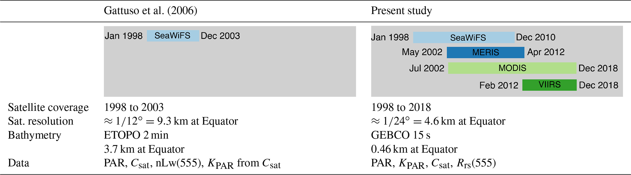
Since these first efforts, new products have become available which can improve estimates of the global distribution of benthic irradiance. These include a much longer time series of ocean color (21 versus 5 years) with an improved spatial resolution (4.6 versus 9.3 km at the Equator). Bathymetric data have also considerably improved since 2006 (0.46 versus 3.7 km at the Equator). Here we make use of these new products to provide a global distribution of photosynthetically available radiation (PAR) reaching the seafloor.

2 Methods

Irradiance, here downwelling irradiance, can be defined or measured at a specific wavelength or integrated within a specific spectral domain. Photosynthetically available radiation (in mol photons m⁻² d⁻¹) is the amount of light available for photosynthesis, which is to say in the 400 to 700 nm spectral range. Biogeochemists and ecophysiologists use the term irradiance for the same quantity. Both terms are used synonymously in the present paper. The characteristics of the products used by Gattuso et al. (2006) and of those in the present study are compared in Table 1.

Table 1 Main characteristics of the products used by Gattuso et al. (2006) and of those in the present study.

2.1 Remote sensing data

Monthly level-3 data of PAR (mol photons m⁻² d⁻¹), K_PAR (m⁻¹), concentration of chlorophyll a (C_sat; mg m⁻³), and remote sensing reflectance at 555 nm (R_rs(555); sr⁻¹) from the satellite-borne sensors SeaWiFS, Moderate Resolution Imaging Spectroradiometer (MODIS), MEdium Resolution Imaging Spectrometer (MERIS), and Visible Infrared Imaging Radiometer Suite (VIIRS) were obtained from the GlobColour project (http://www.globcolour.info, last access: 2 May 2019). The GlobColour project generates global ocean color products by merging data from current and past ocean color instruments (SeaWiFS, MERIS, MODIS, VIIRS, and the two OLCIs), but data retrieved from GlobColour in January 2019 did not comprise data from the Ocean and Land Colour Imager (OLCI). Merged products are generated through a weighted average of the level-2 geophysical products (e.g., chlorophyll) from individual missions. The weights are assigned to each mission under the form of a global uncertainty value derived through validation with respect to global databases of field observations. Alternative products are also generated through the Garver–Siegel–Maritorena (GSM) model (Garver and Siegel, 1997; Maritorena et al., 2002, 2010). The resolution is $\mathrm{1}/{\mathrm{24}}^{\circ }$. Together, the 252 monthly images downloaded (a level-3 image contains values of a product on a regular longitude–latitude grid) cover the period 1998 to 2018.

2.2 Bathymetry and coastline

Depths were estimated from the 2019 General Bathymetric Chart of the Oceans (GEBCO; https://www.gebco.net, last access: 2 May 2019) gridded bathymetry data ($\mathrm{1}/{\mathrm{240}}^{\circ }$ resolution). The coastal zone (0 to 200 m) was determined using a land mask and coastline (Global Self-consistent, Hierarchical, High-resolution Geography, GSHHG) as implemented in the Generic Mapping Tools (GMT; Wessel et al., 2013). The full resolution was used. The Arctic, Antarctic, and nonpolar regions represent, respectively, 24.1 %, 0.6 %, and 75.3 % of the surface area of the coastal zone.

2.3 Case 1 versus Case 2 waters

It is beyond the scope of this paper to review the criteria used to eliminate dubious data when generating a level-3 ocean color composite except for discriminating the water type as being either Case 1 or Case 2 (Morel and Prieur, 1977). In Case 1 waters, where phytoplankton and associated degradation products are the main contributors to light attenuation (but see Claustre and Maritorena, 2003), K_PAR can be modeled as a function of the concentration of chlorophyll a, itself derived from reflectance values. The situation is, however, not as straightforward in Case 2 coastal waters where light attenuation by colored dissolved organic matter and suspended particles other than phytoplankton can be significant and not correlated to the chlorophyll a concentration. The discrimination between these two types is performed at level-2 of the processing, yet it is not considered when generating the level-3 composites (Brian Franz, personal communication, September 2019). Therefore, the average chlorophyll a concentration C_sat in a given bin of a level-3 composite may have been computed over any proportion of Case 1 and Case 2 waters.

The accuracy of C_sat in Case 1 waters is claimed to be ±30 %, whereas it is unknown in Case 2 waters. It is therefore not possible to estimate the accuracy of the chlorophyll product in coastal areas and, in turn, the accuracy of the diffuse attenuation coefficient. The determination of the water type could not be performed with specific algorithms for each water type since no universal algorithm exists for Case 2 waters. It was carried out a posteriori based on the average C_sat and R_rs(555). This determination provides an indication of bins that likely belong to the Case 2 water category when, on average, the individual pixels accumulated in the bins were predominantly of the Case 2 type.

The identification of turbid Case 2 waters has been performed as in Morel and Bélanger (2006) by comparing the water reflectance at 555 nm, R(555), to the maximum value it should have in Case 1 waters and for the same chlorophyll concentration, R_lim(555). Note that the water type was set to Case 1 for any pixel where C_sat<0.2 mg m⁻³ because the algorithm is occasionally prone to falsely classify low-chlorophyll waters as Case 2 (Morel and Bélanger, 2006). Turbid Case 2 waters are those for which R(555)>R_lim(555). To perform this test, R_rs(555) was converted to R(555) as follows (Morel and Gentili, 1996):

$$\begin{array}{}\text{(1)}& R\left(\mathrm{555}\right)=R_{\mathrm{rs}}\left(\mathrm{555}\right)\times Q_{\mathrm{0}}\left(\mathrm{555}\right)/{\mathfrak{R}}_{\mathrm{0}},\end{array}$$

where Q₀(555) is the chlorophyll-dependent Q factor (sr), i.e., the ratio of the upward irradiance to the upwelling radiance (Morel et al., 2002), and ℜ₀ is a term that merges all reflection and refraction effects at the air–sea interface (on average equal to 0.529). Since R_rs(555) is fully normalized (Morel and Gentili, 1996), its dependence on the viewing angle and the sun zenith angle are removed so that both Q and ℜ are taken for a nadir view and a sun at zenith (hence the “0” subscript).

2.4 Benthic irradiance

K_d(λ₀,z), the diffuse attenuation coefficient for the downward irradiance (E_d) for a given wavelength (λ₀), describes the exponential attenuation of irradiance with depth in the water column. It determines the amount of radiation reaching a given depth (z):

$$\begin{array}{}\text{(2)}& K_{\mathrm{d}}({\mathit{\lambda }}_{\mathrm{0}},z)={\displaystyle \frac{-\partial \ln \left(E_{\mathrm{d}}\right({\mathit{\lambda }}_{\mathrm{0}},z\left)\right)}{\partial z}}.\end{array}$$

The spectral composition of the radiation is not considered in this work, and only its integral value between 400 and 700 nm is used (i.e., the photosynthetically available radiation, PAR). The attenuation coefficient for PAR is therefore

$$\begin{array}{}\text{(3)}& K_{\mathrm{PAR}}\left(z\right)={\displaystyle \frac{-d\ln \left(\mathrm{PAR}\right(z\left)\right)}{\mathrm{d}z}}.\end{array}$$

The average value (K_PAR) of K_PAR(z) over the euphotic zone, approximated as the depth where PAR is reduced to 1 % of its value just beneath the sea surface, is computed from the corresponding chlorophyll concentration for Case 1 waters C_sat and K_d(490) using the following equations (Morel et al., 2007; ACRI-ST GlobColour Team, 2017):

$$\begin{array}{}\text{(4)}& {\displaystyle }{K}_{\mathrm{d}}\left(\mathrm{490}\right)=\mathrm{0.0166}+\mathrm{0.08349}\times C_{\mathrm{sat}}^{\mathrm{0.63303}},\text{(5)}& {\displaystyle }\begin{array}{rl}{K}_{\mathrm{PAR}}& =\mathrm{0.0665}+\mathrm{0.874}\times K_{\mathrm{d}}\left(\mathrm{490}\right)\\ & -\mathrm{0.00121}/K_{\mathrm{d}}\left(\mathrm{490}\right).\end{array}\end{array}$$

The irradiance at the bottom depth (z_B) is then calculated as follows.

$$\begin{array}{}\text{(6)}& {\mathrm{PAR}}_{\mathrm{B}}=\exp (-K_{\mathrm{PAR}}\times z_{\mathrm{B}})\end{array}$$

• For the nonpolar region, all months are taken into account, so we have 21 years ×12 months =252 values by pixel at most.

• For the Arctic region, months 6–10 (June–October) are taken into account, so we have 21 years ×5 months =105 values by pixel at most.

• For the Antarctic region, months 1–3 and 11–12 (January–March and November–December) are taken into account, so we have 21 years ×5 months =105 values by pixel at most.

• In total, we have 252 monthly PAR_B images for the nonpolar region and 105 for the Arctic and Antarctic regions.

The product delivered comprises longitude, latitude, depth, area, PAR, K_PAR, and PAR_B for each coastal pixel. PAR, K_PAR, and PAR_B are monthly climatologies or a climatology over the entire time series (see Sect. 4). The calculation of surface area receiving PAR_B above a certain threshold does not use these climatologies.

2.5 Surface area receiving light above a certain threshold

Calculations of surface area receiving PAR_B above a certain threshold are made in two steps. First a 𝒫 function is calculated with the available pixels. Then the area is calculated as the product of the 𝒫 function by the surface of the coastal zone (0–200 m).

2.5.1 The three main regions

A region is defined here by an interval of latitude at the surface of the Earth. Polar regions are more frequently observed by satellites, yet polar night and cloudiness end up with data not being available for several months of the year. So three regions have been defined:

• the “nonpolar” region (60^∘ S; 60^∘ N), for which data are always available;

• the “Arctic” region (60^∘ N; 90^∘ N), for which data are available during the months of June, July, August, September, and October;

• the “Antarctic” region (90^∘ S; 60^∘ S), for which data are available during the months of January, February, March, November, and December.

2.5.2 𝒫 functions

Definition of a 𝒫 function for a monthly PAR_B image of a region

• Let I be the monthly image (values of PAR_B on the floor of the coastal zone of the region).

• Let S_a,I be the available surface, i.e., the total surface of pixels for which an irradiance value is available (varying every month).

• Let E be a value of irradiance (expressed in mol photons m⁻² d⁻¹).

• Let s_I(E) be the total surface of pixels collecting irradiance greater than E.

• Let the 𝒫_I function be defined as ${\mathcal{P}}_I\left(E\right)=\mathrm{100}{s}_I\left(E\right)/S_{\mathrm{a},I}$.

Definition of a climatological 𝒫 function

Our purpose is now to define a 𝒫 function for a set of monthly values $\mathcal{I}=\mathit{\{}{I}_i,i=\mathrm{1}\mathrm{\dots }n\mathit{\}}$. Giving a value of irradiance E, it is defined as follows:

$$\begin{array}{}\text{(7)}& {\mathcal{P}}_{\mathcal{I}}\left(E\right)=\mathrm{100}\sum _{i=\mathrm{1}}^n{s}_{I_i}\left(E\right)/\sum _{i=\mathrm{1}}^n{S}_{\mathrm{a},I_i}.\end{array}$$

Climatological monthly 𝒫 function

In this case, the 21 data sets available for a given month through the entire time series (1998 to 2018) are selected to calculate the 𝒫 function according to Eq. (7). So we have the following:

• 12 climatological monthly 𝒫 functions for the nonpolar region;

• 5 climatological monthly 𝒫 functions for the Arctic region;

• 5 climatological monthly 𝒫 functions for the Antarctic region.

Climatological global 𝒫 function

The global 𝒫 function (𝒫_g) is obtained using all data sets (252 for nonpolar and 105 for Arctic and Antarctic regions) in Eq. (7).

Table 2 Surface area (S) of coastal waters (depth <200 m) of different optical characteristics. Calculations were performed on monthly products. Values reported by Gattuso et al. (2006) are shown in parentheses for comparison. Gattuso et al. (2006) did not report data for the Antarctic.

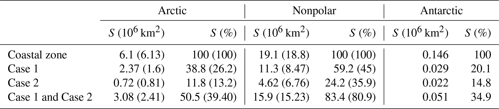
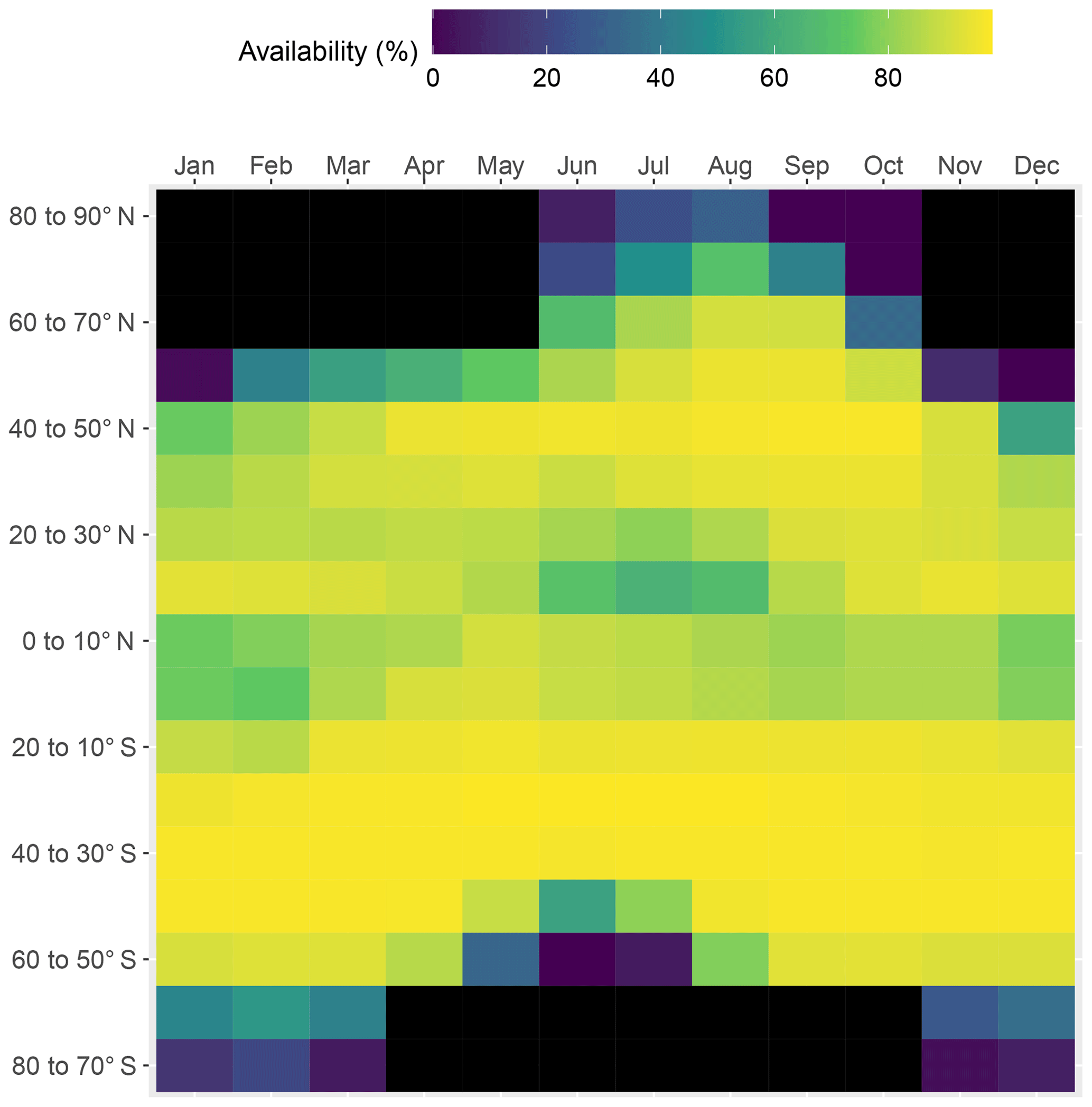
Figure 1 Availability of remote sensing data over the 21 year time series. Availability is expressed as the monthly mean of the percent area of each latitudinal band covered by the satellite.

𝒫 functions for a subregion

A subregion may be defined within one of the three main regions. In this case, data sets are clipped according to the subregion's boundaries, and the months used are those of the main region. Calculation is identical to that described above for the climatological global 𝒫 function (Sect. 2.5.6). The R package CoastalLight (see Sect. 4) can be used to calculate a 𝒫 function for a subregion with the help of a remote server.

2.5.3 Surface areas

Let 𝒫 be the 𝒫 function of the zone and S_geo its area; the area receiving irradiance above a threshold E is

$$\begin{array}{}\text{(8)}& s\left(E\right)=S_{\mathrm{geo}}{\displaystyle \frac{\mathcal{P}\left(E\right)}{\mathrm{100}}}.\end{array}$$

3 Results and discussion

The present study essentially confirms the bathymetric data reported in our earlier study (Gattuso et al., 2006) but shows substantial differences in the optical data.

3.1 Surface area and depth of subregions of the ocean

The area and depth of the three regions measured with the most recent GEBCO bathymetry are very similar to those obtained with the coarser ETOPO2 data set used by Gattuso et al. (2006) (Table 2). The surface area of the ocean with depth less than 200 m is 25.3×10⁶ km². Three geographical areas are considered: the Arctic (60 to 90^∘ N), the nonpolar region (60^∘ N to 60^∘ S), and the Antarctic (60 to 90^∘ S) regions, respectively covering 24.1 %, 75.5 %, and 0.6 % of the global coastal zone. The average depth of the coastal zone is almost twice as much in the Antarctic than in the Arctic and nonpolar regions (137 versus 77 and 71 m).

Table 3 Surface area and average depth of the various pixel classes. Calculations were performed on monthly data sets for the periods indicated. Values reported by Gattuso et al. (2006) are shown in parentheses for comparative purposes. Gattuso et al. (2006) did not report data for the Antarctic. Z_1 % is the depth at which benthic irradiance or benthic PAR (PAR_B) equals 1 % of surface irradiance or PAR. Available pixels are the pixels for which PAR, K_PAR, C_sat, and R_rs(555) are available for analysis.

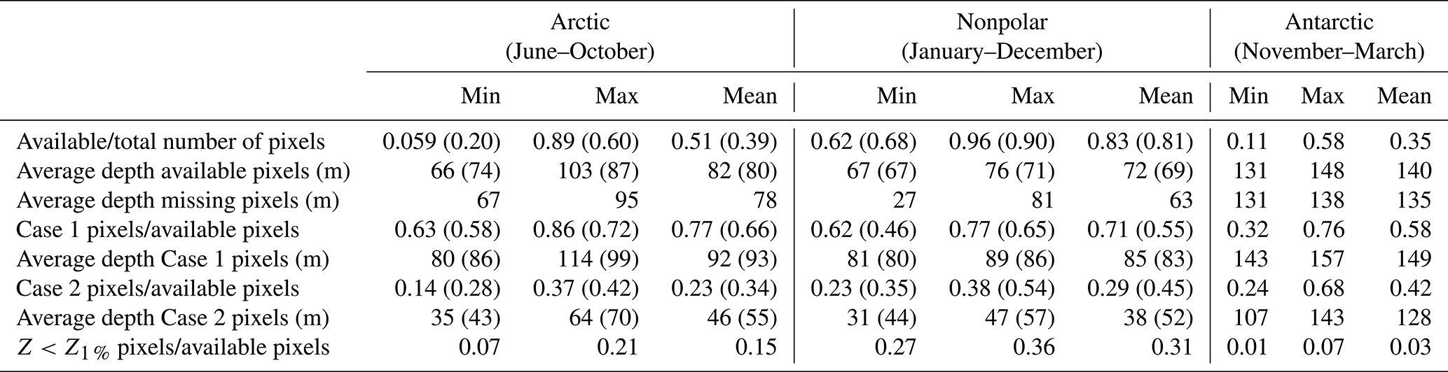
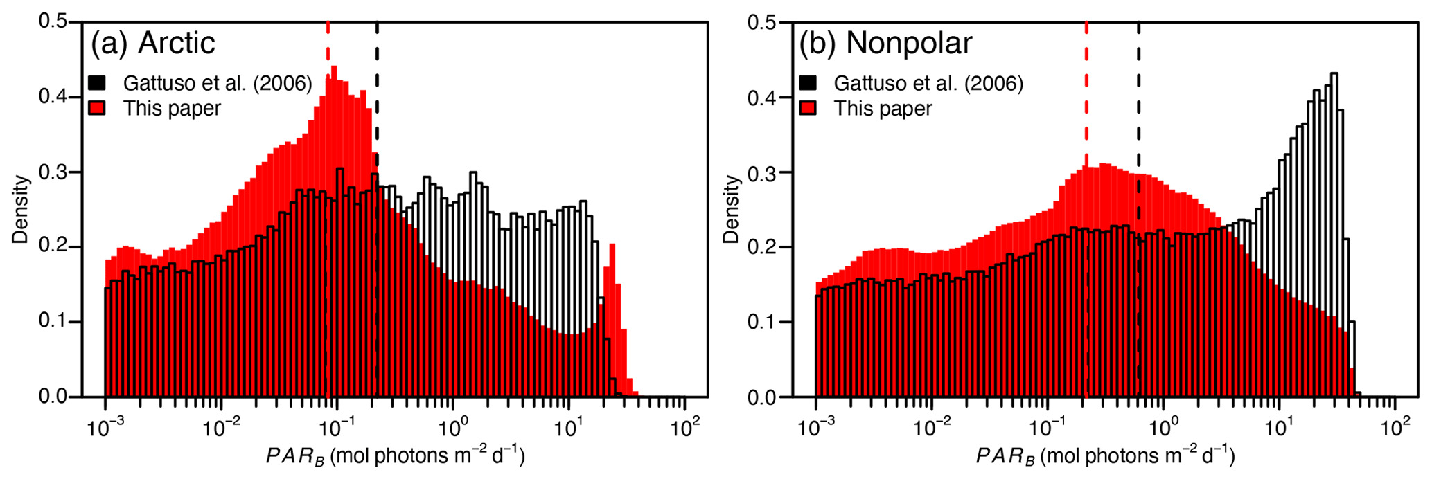
Figure 2 Distribution of PAR_B in the Arctic (a) and nonpolar (b) regions in the present study and in Gattuso et al. (2006). The dashed vertical lines represent the median values in Gattuso et al. (2006) (black) and the present (red) studies.

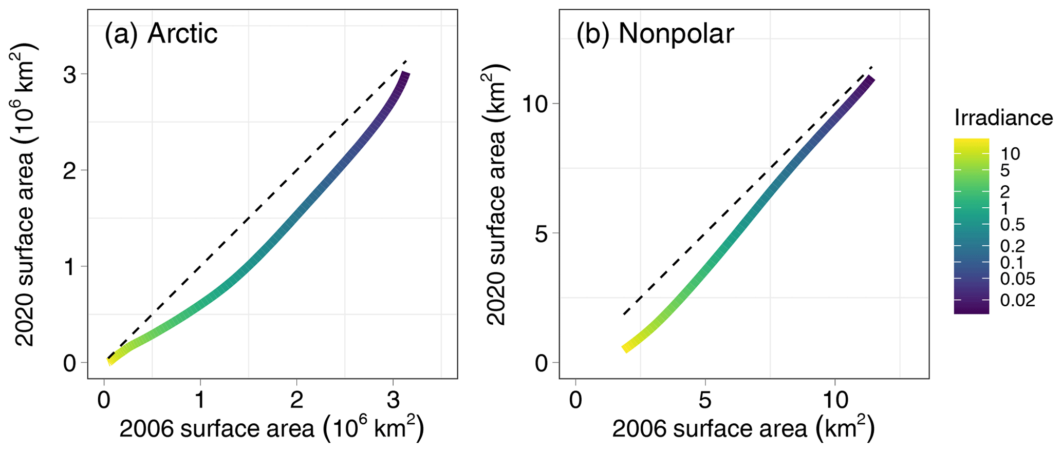
Figure 3 Comparison of the surface area of the seafloor of the Arctic (a) and nonpolar (b) regions receiving an irradiance larger than a threshold value ranging from 0.01 to 20 mol photons m⁻² d⁻¹ calculated in the present paper (2020) compared with the surface area reported by Gattuso et al. (2006). The dotted line is the 1:1 relationship.

3.2 Availability of ocean color data and seawater types

The availability of monthly ocean color data is highly variable depending on the latitude and month of the year (Fig. 1). It is highest in nonpolar regions where, on average, data are available in 83 % (range: 62 %–96 %) of the pixels in monthly data sets. In the Arctic and the Antarctic, sunlight is available only during the 5 summer months of the year, i.e., June to October and November to March, respectively. Furthermore, data availability is higher in midsummer than in early and late summer (Fig. 1). Data availability also decreases as one gets closer to the poles. On average, data are available for 51 % and 35 % of the summer data sets in the Arctic and Antarctic regions (ranges: 6 %–89 % and 11 %–58 %, respectively; Table 3). Data availability is higher in the present study which used multiple sensors compared to a previous study that only used SeaWiFS data (Gattuso et al., 2006). Several factors contribute to the lower availability of data in polar regions: pixels are contaminated by sea ice and flagged accordingly, high occurrence of cloudy days, and low incidence of the sun.

The coverage of the Arctic has improved by about 20 % more pixels with available data (Table 3). Case 1 and Case 2 waters are approximately equally distributed in the Antarctic region (Table 2). In contrast, there is a clear dominance of Case 1 over Case 2 waters (70 % versus 30 %) in the nonpolar region, whereas it was more even (55 % versus 45 %) in Gattuso et al. (2006). This discrepancy may be due to the different approaches used to differentiate between Case 1 and Case 2 waters. The present study uses the remote sensing reflectance at 555 nm, R_rs(555), provided by the GlobColour project, whereas it was roughly estimated from the normalized water-leaving radiance in the previous study (Eq. 1 in  Gattuso et al., 2006). The quality of the results should therefore have improved. In any case, the usefulness of this distinction is relatively limited because the light penetration through the water column is calculated in the same way in the two cases. The distribution of water quality is, however, useful to estimate the reliability of the bottom irradiance which is much better in Case 1 waters than in Case 2 waters. The average depth of the missing pixels is similar to that of the available pixels in the Arctic and Antarctic regions (Table 3). However, it is sometimes lower in the nonpolar region. The lowest values occur when the amount of available pixels is the largest (data not shown), suggesting that the missing pixels are preferentially located close to the coastline.

3.3 Bottom irradiance

The distribution of PAR_B has changed in the present study compared to Gattuso et al. (2006), with less irradiance values above 0.2 mol photons m⁻² d⁻¹ and more irradiance values around 0.1 mol photons m⁻² d⁻¹ in the present study than in Gattuso et al. (2006) (Fig. 2).

The surface area of the seafloor receiving an irradiance larger than a threshold value is lower than in the previous estimate of Gattuso et al. (2006) (Fig. 3). Differences are low below an irradiance threshold of 0.2 mol photons m⁻² d⁻¹ – 3 % to 16 % lower, respectively, in the nonpolar and Arctic regions. However, differences are as high as 26 % and 56 %, respectively, in the nonpolar and Arctic regions for irradiance thresholds ranging between 10 and 50 mol photons m⁻² d⁻¹. Such differences can be due to several causes.

The present study and Gattuso et al. (2006) used different approaches. In the 2006 study, a 𝒫 function was derived for each month and then monthly means calculated, implicitly giving the same weight to each month irrespective of the number of pixels with available data. In the present study, each month has a weight proportional to the surface area for which data are available, hence providing better estimates. Second, there are more data available in the data set compiled in the present paper, especially in the Arctic. Third, Gattuso et al. (2006) fitted polynomial functions on the relationship between irradiance and the cumulative surface area of the seafloor receiving irradiance above a prescribed threshold. These functions only provide rough estimates and are not used in the present study. The R package CoastalLight has been developed in the present study to provide more accurate estimates (Sect. 4) calculated from the underlying data, which is to say the number of pixels and their size.

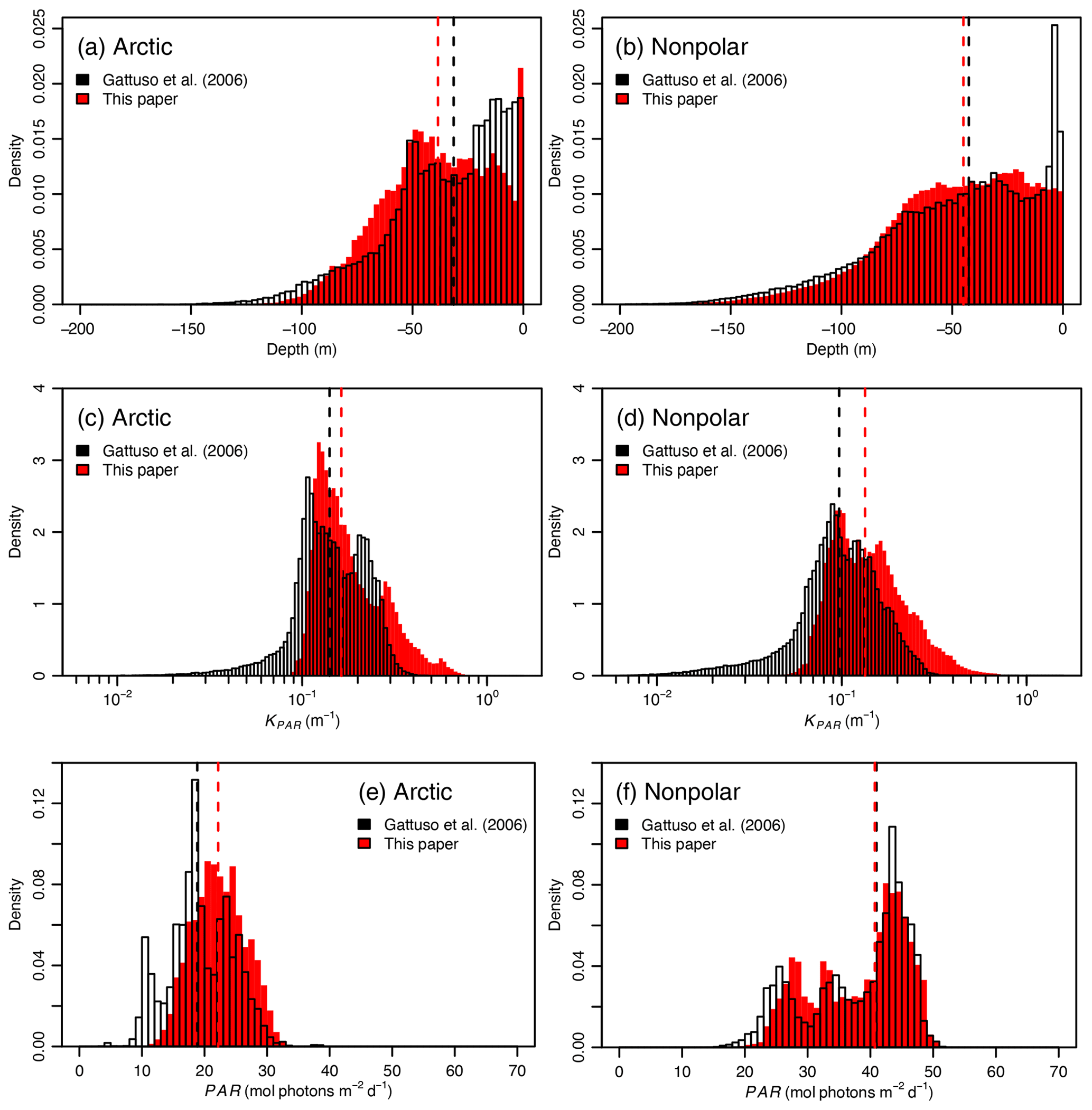
Figure 4 Distribution of depth, K_PAR, and PAR in the present study and in Gattuso et al. (2006). The dashed vertical lines represent the median values in the 2006 (black) and present (red) studies.

Table 4 Median values of key variables used by Gattuso et al. (2006) and the present study.

These changes in approach, together with the different data sets used for the optical and bathymetric data, have led to significant changes in three factors that affect bottom PAR (PAR_B; Fig. 4; Table 4). Two of them contribute to a decline of PAR_B: (1) a change in the depth distribution leading to an increase in the median depth (39 versus 31 m) and (2) a distribution of K_PAR that moved towards higher values in the present study. Also, (3) surface PAR tends to be higher in the present study than in the previous one. We do not have any independent confirmation of such an increase in surface PAR globally. The change could be real but could also result from successive reprocessing of the individual sensor archives that make up the GlobColour products that have been performed since 2006. This reprocessing indeed includes updates of calibration coefficients and possible refinements of algorithms. The combined effects of the first two causes are larger that the effect of the third one, explaining why bottom PAR is overall smaller in the present study than in the previous one (Gattuso et al., 2006).

3.4 Implications for the distribution of photosynthetic organisms and communities

The differences in PAR_B between the 2006 study and the present one have implications on the potential surface areas receiving enough irradiance to sustain growth of photosynthetic organisms and communities (Table 5). Surface areas are 4 % to 47 % lower in the present study depending on the region and organism or community considered. As shown in Fig. 3, in the nonpolar region, the higher the irradiance threshold, the larger the difference. Hence, the differences are generally reasonable (less than 15 %) for organisms but higher (up to 47 %) for communities which have higher light requirements to maintain positive rates of net primary production. Differences between the 2006 estimates and the present ones are generally larger in the Arctic than in the nonpolar region for organisms and fairly similar for communities.

Table 5 Top: Organisms. Surface area (percent of the coastal zone) where irradiance does not limit the distribution of photosynthetic organisms. Values reported by Gattuso et al. (2006) are shown in parentheses for comparative purposes. The irradiance thresholds are the first deciles of the minimum light requirements compiled by Gattuso et al. (2006). Data are not reported in the Arctic region for seagrasses and scleractinian (reef-building) corals where these groups are not present. Bottom: Communities. Surface area (percent of the coastal zone) where benthic irradiance is higher that the daily community compensation irradiance (net primary production >0). The irradiance thresholds are the first deciles of the minimum light requirements compiled by Gattuso et al. (2006). Data are not reported for seagrass communities and coral reefs in the Arctic and Antarctic regions where they do not occur.

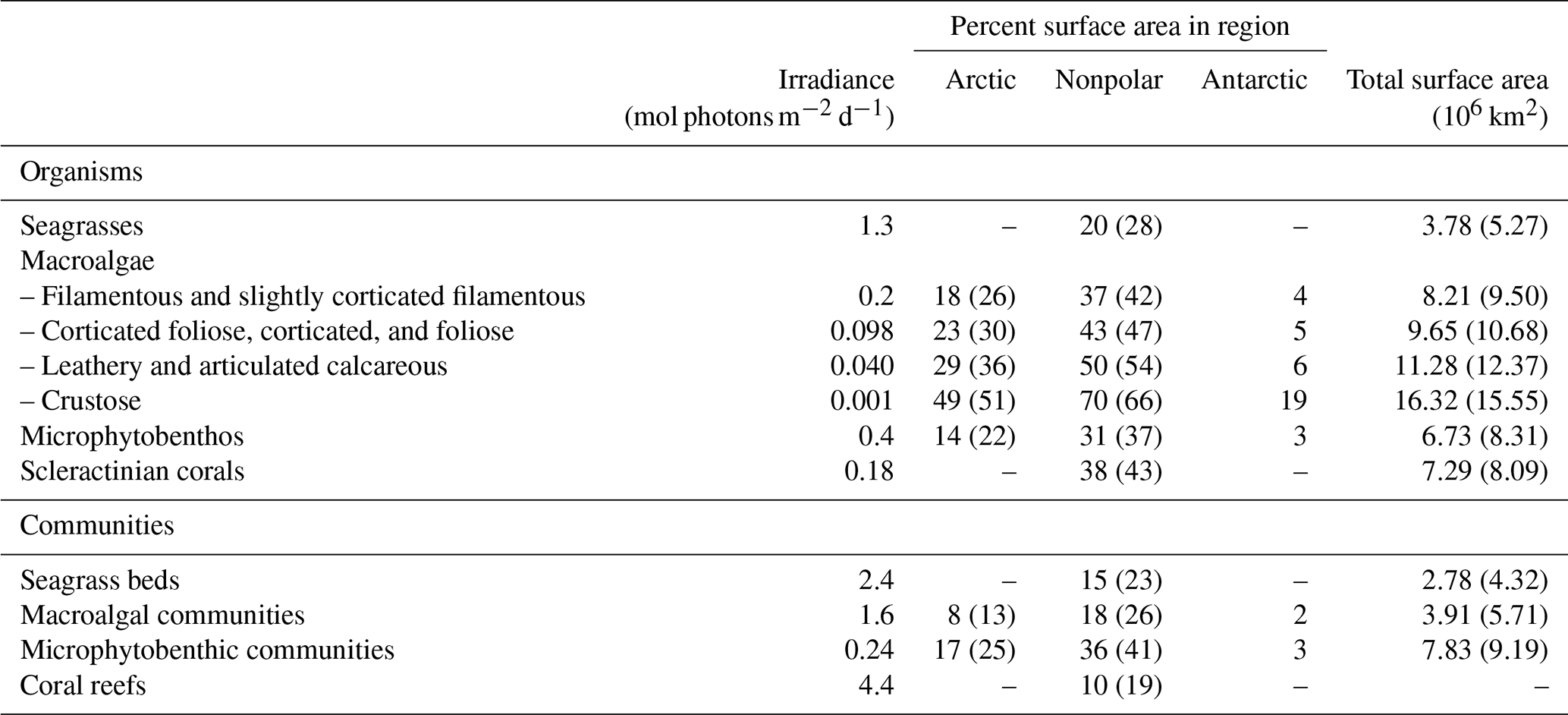
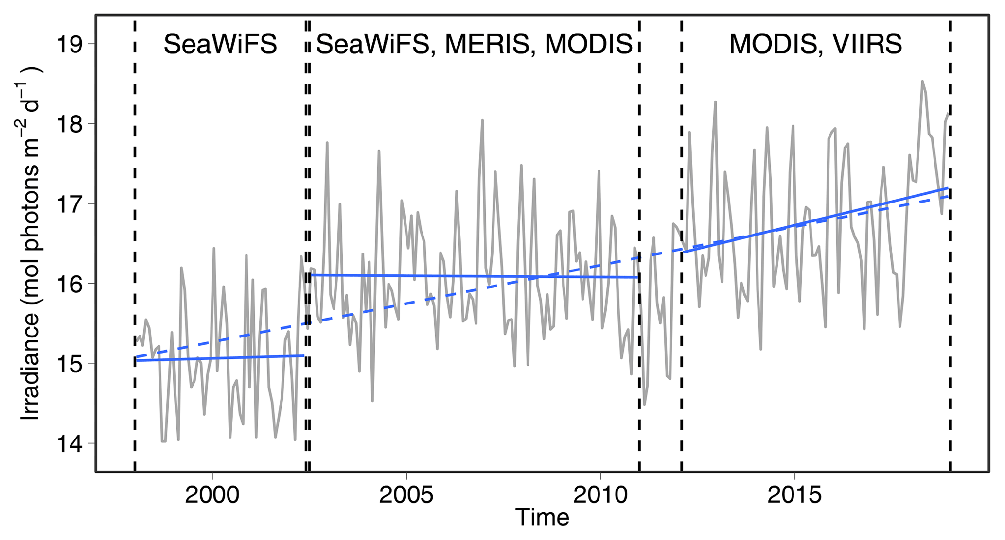
Figure 5 Time series of the surface area (percent) of the coastal nonpolar region receiving more than 2 mol photons m⁻² d⁻¹. The linear regression between 1999 and 2018 is shown as a dashed line, while the result of separate linear regressions for the three time periods with the same set of ocean color sensors is shown as a solid line.

3.5 Analysis of time series

Long-term changes in the optical characteristics have recently been described. For example, using SeaWiFS monthly global ocean transparency data from September 1997 to November 2010, He et al. (2017) described a rapid decrease in global mean ocean transparency at a rate of −0.85 m yr⁻¹ between 1997 and 1999, followed by a small increase with a rate of 0.04 m yr⁻¹ between 2000 and 2010.

In the Arctic coastal zone, significant climate change effects have been observed over the last 2 decades including enhanced melting of sea ice during the summer period, permafrost thaw, and an increase in river discharge into the Arctic Ocean. Time series of ocean color satellite data have been successfully used to confirm these changes and quantify an increase of up to 40 % in the concentrations of both dissolved and particulate terrestrial substances in Arctic coastal waters (Doxaran et al., 2015; Atsushi Matsuoka, personal communication, June 2019). In nonpolar regions, satellite observations did not reveal such a significant temporal trend (e.g., Loisel et al., 2014) but often highlighted how human-induced activities have an impact on the discharge of big rivers and the consequences on the turbidity of surrounding coastal waters (e.g., Feng et al., 2014).

With a time series 21 years long, it is tempting to investigate whether long-term changes in PAR_B can be identified. Figure 5 shows the percent surface area of the coastal zone of the nonpolar region receiving 2 mol photons m⁻² d⁻¹ or more. There is a highly significant trend with an increase in the percent of surface area by 0.1±0.02 % yr⁻¹ (± 99 % confidence interval). However, separate regression analyses show data shifts occur between the three time periods when the same ocean color sensors were in operation. The trends are therefore highly variable during specific time periods corresponding to various sets of ocean color sensors. We conclude that no long-term trend in PAR_B can be identified in this data set.

4 Data availability

The geographical and optical data generated and used in this paper are openly available at the World Data Center PANGAEA (Gentili and Gattuso, 2020a; https://doi.org/10.1594/PANGAEA.910898). They consist of 14 netCDF files with a unique dimension (the coastal pixel number) which is identical for all files:

• a netCDF file with geographical information (latitude, longitude, depth, area of the pixels) (CoastalLight_geo.nc; about 1.2 Gb);

• a netCDF file with the climatology over the whole 21 year period calculated as the mean values of the monthly data of PAR, K_PAR, and PAR_B (CoastalLight_00.nc; about 1.1 Gb);

• 12 netCDF files with monthly climatologies (mean of the values of PAR, K_PAR and PAR_B).

The 12 netCDF files include the following:

• Monthly climatology, January: CoastalLight_01.nc (6.2 Gb);

• Monthly climatology, February: CoastalLight_02.nc (6.8 Gb);

• Monthly climatology, March: CoastalLight_03.nc (7 Gb);

• Monthly climatology, April: CoastalLight_04.nc (7 Gb);

• Monthly climatology, May: CoastalLight_05.nc (7 Gb);

• Monthly climatology, June: CoastalLight_06.nc (9.6 Gb);

• Monthly climatology, July: CoastalLight_07.nc (10.6 Gb);

• Monthly climatology, August: CoastalLight_08.nc (11 Gb);

• Monthly climatology, September: CoastalLight_09.nc (10.4 Gb);

• Monthly climatology, October: CoastalLight_10.nc (7.8 Gb);

• Monthly climatology, November: CoastalLight_11.nc (6.4 Gb);

• Monthly climatology, December: CoastalLight_12.nc (6 Gb).

The surface area of three regions (Arctic, Antarctic, and nonpolar) receiving an irradiance above a certain threshold is available using the R package CoastalLight (https://github.com/jpgattuso/CoastalLight, Gentili and Gattuso, 2020b). The package can be installed and used as follows:

• install.packages(“devtools”)

• library(devtools)

• install_github(“jpgattuso/CoastalLight”)

• use function cl_surface of the CoastalLight package.

The surface area of a subregion of one of the regions above receiving an irradiance above a certain threshold can be derived as follows (complete information can be found in the documentation of the CoastalLight package):

• connecting to the web server http://obs-vlfr.fr/Pfunction/ (last access: 30 July 2020) to calculate and download its 𝒫 function;

• then using this 𝒫 function with function cl_surface of the CoastalLight package.

5 Conclusions

This study builds on the first, and still only, global distribution of photosynthetically available radiations reaching the seafloor (Gattuso et al., 2006). It improves the geographical and depth resolutions and covers a much longer period of time. Despite these key improvements, several limitations inherent to the approach remain. While the spatial resolution is twice better than the previous products, 4.6 km at the Equator, it is still coarse for investigating the distribution and function of organisms and communities which change at much finer scales. The parameterization used to convert reflectance data to irradiance is approximate in Case 2 waters. Finally, light absorption in the benthic nepheloid layer is not taken into consideration. The global distribution of PAR_B we provide is derived from state-of-the-art data and computations and is arguably the best that can be offered at this time. Despite its shortcomings, it should considerably improve estimates of the geographical and depth distributions of photosynthetic organisms and ecosystems and help assess their contribution to global biogeochemical cycles.

Appendix A: Graphical representation of 𝒫 functions

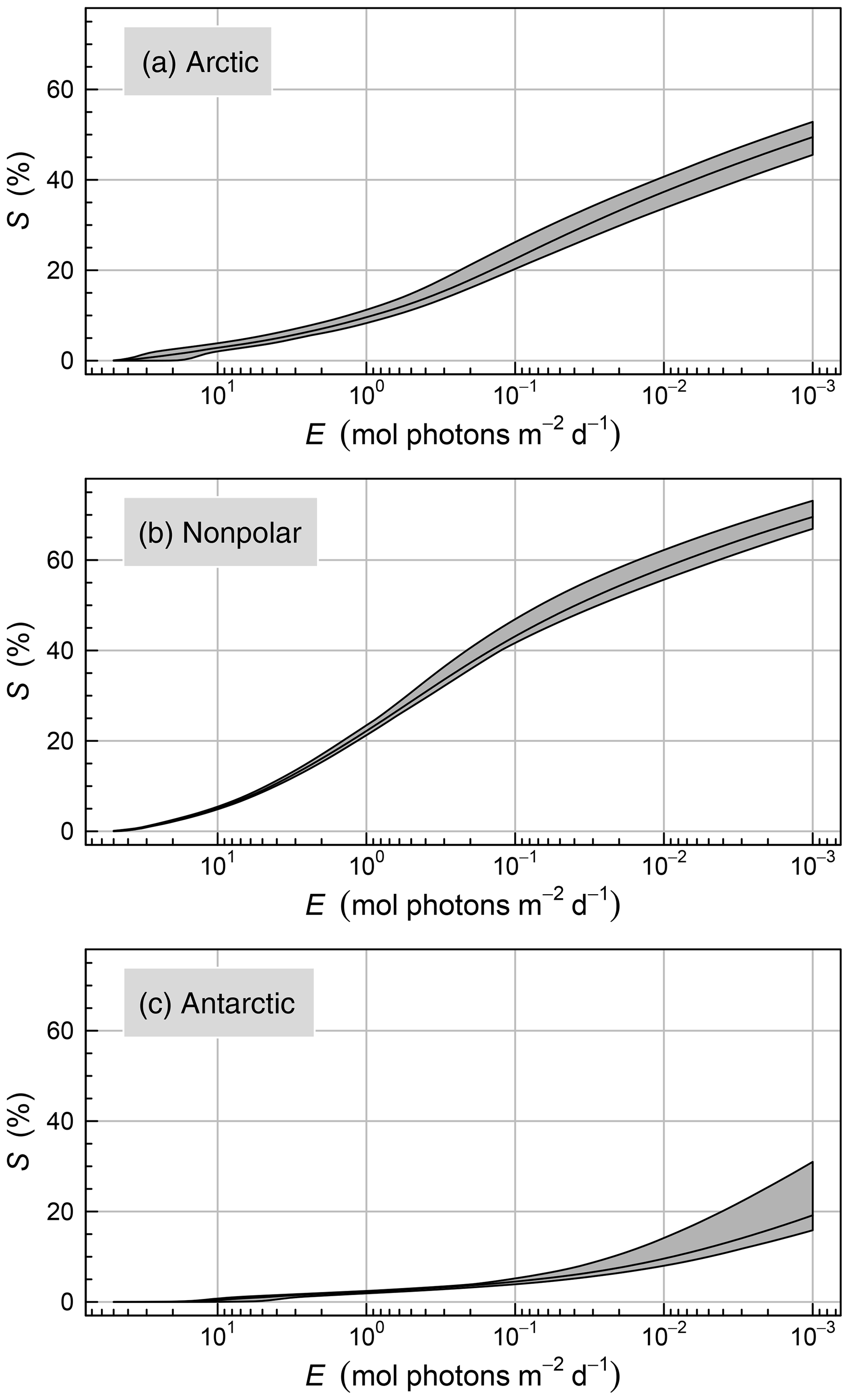
Figure A1 Cumulative surface area of the seafloor (S) receiving irradiance above a prescribed threshold (E). Data are expressed in percent of the total surface area of each region (19 080 010, 6 100 532, and 146 171 km², respectively, for the nonpolar, Arctic, and Antarctic regions). The shaded areas show the monthly variability.