the Creative Commons Attribution 4.0 License.
the Creative Commons Attribution 4.0 License.
 | 16 Jul 2020
Radiative forcing of climate change from the Copernicus reanalysis of atmospheric composition
Nicolas Bellouin
Will Davies
Keith P. Shine
Johannes Quaas
Johannes Mülmenstädt
Piers M. Forster
Chris Smith
Lindsay Lee
Leighton Regayre
Guy Brasseur
Natalia Sudarchikova
Idir Bouarar
Olivier Boucher
Gunnar Myhre
Radiative forcing provides an important basis for understanding and predicting global climate changes, but its quantification has historically been done independently for different forcing agents, has involved observations to varying degrees, and studies have not always included a detailed analysis of uncertainties. The Copernicus Atmosphere Monitoring Service reanalysis is an optimal combination of modelling and observations of atmospheric composition. It provides a unique opportunity to rely on observations to quantify the monthly and spatially resolved global distributions of radiative forcing consistently for six of the largest forcing agents: carbon dioxide, methane, tropospheric ozone, stratospheric ozone, aerosol–radiation interactions, and aerosol–cloud interactions. These radiative-forcing estimates account for adjustments in stratospheric temperatures but do not account for rapid adjustments in the troposphere. On a global average and over the period 2003–2017, stratospherically adjusted radiative forcing of carbon dioxide has averaged +1.89 W m−2 (5 %–95 % confidence interval: 1.50 to 2.29 W m−2) relative to 1750 and increased at a rate of 18 % per decade. The corresponding values for methane are +0.46 (0.36 to 0.56) W m−2 and 4 % per decade but with a clear acceleration since 2007. Ozone radiative-forcing averages +0.32 (0 to 0.64) W m−2, almost entirely contributed by tropospheric ozone since stratospheric ozone radiative forcing is only +0.003 W m−2. Aerosol radiative-forcing averages −1.25 (−1.98 to −0.52) W m−2, with aerosol–radiation interactions contributing −0.56 W m−2 and aerosol–cloud interactions contributing −0.69 W m−2 to the global average. Both have been relatively stable since 2003. Taking the six forcing agents together, there is no indication of a sustained slowdown or acceleration in the rate of increase in anthropogenic radiative forcing over the period. These ongoing radiative-forcing estimates will monitor the impact on the Earth's energy budget of the dramatic emission reductions towards net-zero that are needed to limit surface temperature warming to the Paris Agreement temperature targets. Indeed, such impacts should be clearly manifested in radiative forcing before being clear in the temperature record. In addition, this radiative-forcing dataset can provide the input distributions needed by researchers involved in monitoring of climate change, detection and attribution, interannual to decadal prediction, and integrated assessment modelling. The data generated by this work are available at https://doi.org/10.24380/ads.1hj3y896 (Bellouin et al., 2020b).
- Article
(3955 KB) - Full-text XML
- BibTeX
- EndNote


Human activities have profoundly modified the composition of the Earth's atmosphere. They have increased the concentrations of greenhouse gases, with concentrations of carbon dioxide increasing from 278 to 407 ppm (an increase of 46 %) and methane from 722 to 1858 ppb (+157 %) over the period 1750–2018 (Dlugokencky et al., 2019). Concentrations of aerosols and tropospheric ozone (Hartmann et al., 2013) are frequently above pre-industrial levels in many regions, especially those that are the most densely populated. The stratospheric ozone layer is only beginning its recovery after being affected by emissions of man-made ozone-depleting substances in the 1970–1980s (WMO, 2018). Those modifications have important impacts on human health and prosperity and on natural ecosystems. One of the most adverse effects of human modification of atmospheric composition is climate change.
A perturbation to the Earth's energy budget leads to temperature changes and further climate responses. The initial top-of-atmosphere imbalance is the instantaneous radiative forcing. Several decades ago, it was realised that for comparison of climate change mechanisms the radiative flux change at the tropopause, or equivalently at the top of the atmosphere after stratospheric temperatures are adjusted to equilibrium, was a better predictor for the surface temperature change and defined as radiative forcing (RF) (Ramanathan, 1975; Shine et al., 1990; Ramaswamy et al., 2019). The adjustment time in the stratosphere is of the order of 2 to 3 months and is several orders of magnitude shorter than the time required for the surface–tropospheric system to equilibrate after a (time-independent) perturbation. More recently the effective radiative forcing (ERF) has been defined to include rapid adjustments, where, in addition to the stratospheric temperature adjustment, these adjustments occur due to heating or cooling of the troposphere in the absence of a change in the ocean surface temperature (Boucher et al., 2013; Myhre et al., 2013a; Sherwood et al., 2015; Ramaswamy et al., 2019). For certain climate change mechanisms, especially those involving aerosols, the rapid adjustments are important, but in many cases, notably the well-mixed greenhouse gases, RF is relatively similar to ERF (Smith et al., 2018a). In principle, the ERF is a better predictor of surface temperature change than RF but is less straightforward to quantify for all forcing mechanisms (see, e.g. Ramaswamy et al., 2019). The quantification of RF has been a central part of every Assessment Report of the Intergovernmental Panel on Climate Change (IPCC) (Shine et al., 1990; Schimel et al., 1996; Ramaswamy et al., 2001; Forster et al., 2007; Myhre et al., 2013a).
Carbon dioxide, methane, and ozone exert an RF by absorbing and emitting longwave (LW), or terrestrial, radiation and absorbing shortwave (SW), or solar, radiation. Aerosols exert an RF directly by scattering and absorbing shortwave and longwave radiation, a process called aerosol–radiation interactions (ari; Boucher et al., 2013). Aerosols also exert an RF indirectly through their roles as cloud condensation nuclei (CCN), which regulate cloud droplet number concentration and therefore cloud albedo. Those processes are called aerosol–cloud interactions (aci; Boucher et al., 2013). Quantifying RF is a difficult task. It strongly depends on the horizontal and vertical distributions of the forcing agents, which in the case of ozone and aerosols are very heterogeneous. It depends on the ability of forcing agents to interact with radiation, which is difficult to characterise well in the case of chemically diverse species like aerosols (Bellouin et al., 2020a) or may be incompletely represented in many radiative-transfer codes (e.g. Collins et al., 2006; Etminan et al., 2016). RF is defined with respect to an unperturbed state, typically representing pre-industrial (PI) conditions, which is very poorly known for the short-lived forcing agents like ozone and aerosols (Myhre et al., 2013a; Carslaw et al., 2013). RF also depends on the ability to understand and calculate the distributions of radiative fluxes with accuracy (Soden et al., 2018), including the contributions of clouds and the surface. Those difficulties translate into persistent uncertainties attached to IPCC radiative-forcing estimates. Those difficulties are compounded by the lack of consistent and integrated quantifications across forcing agents. In the IPCC Fifth Assessment Report (AR5) (Myhre et al., 2013a), carbon dioxide and methane radiative forcing were derived from fits to line-by-line radiative-transfer models (Myhre et al., 1998) using global-mean changes in surface concentrations as input. Aerosol radiative forcing from interactions with radiation was based on global modelling inter-comparisons (Myhre et al., 2013b; Shindell et al., 2013a) and observation-based estimates (Bond et al., 2013; Bellouin et al., 2013). Aerosol radiative forcing from interactions with clouds was based on many satellite- and model-based studies (Boucher et al., 2013). Ozone radiative forcing was based on results from the Atmospheric Chemistry and Climate Model Intercomparison Project (ACCMIP) (Stevenson et al., 2013; Conley et al., 2013).
The development of observing and modelling systems able to monitor and forecast changes in atmospheric composition offers an attractive way to alleviate some of these difficulties. One of those systems is the reanalysis routinely run by the Copernicus Atmosphere Monitoring Service (CAMS; Inness et al., 2019), which crowns more than a decade of scientific endeavours (Hollingsworth et al., 2008) rendered possible by the impressive increase in observing capabilities and numerical weather prediction over the past 40 years (Bauer et al., 2015). The CAMS reanalysis combines, in a mathematically optimal way, many diverse observational data sources (see Table 2 of Inness et al., 2019) from ground-based and space-borne instruments, with a numerical weather prediction model (see Table 1 of Inness et al., 2019) that also represents the sources and sinks of carbon dioxide and methane and the complex chemistry governing the concentrations of ozone and aerosols. Reanalysis products therefore give a complete and consistent picture of the atmospheric composition of the past, covering in the case of CAMS the period 2003 to the present. Reanalysis products are therefore a robust basis for estimating RF of climate change.
This article describes the RF estimates of carbon dioxide, methane, aerosol, and ozone made as part of the CAMS from its reanalysis of atmospheric composition. The article starts by describing the methods used to estimate RF from the reanalysis in Sect. 2, before discussing how the PI reference state is estimated for the different forcing agents in Sect. 3. Section 4 describes the estimates of uncertainties in CAMS RF. Section 5 presents the results over the period 2003–2017, discussing distributions and temporal rate of change and comparing these to previous estimates from the IPCC. Section 6 concludes by describing potential uses for the CAMS radiative-forcing products and outline further research avenues that would improve the estimates further.
CAMS estimates follow the definitions for instantaneous and stratospherically adjusted RF given in the IPCC AR5 (Myhre et al., 2013a).
-
Instantaneous RF (IRF) is the “instantaneous change in net (down minus up) radiative flux (shortwave plus longwave; in W m−2) due to an imposed change.”
-
Stratospherically adjusted RF (hereafter simply referred to as RF) is “the change in net irradiance at the tropopause after allowing for stratospheric temperatures to readjust to radiative equilibrium, while holding surface and tropospheric temperatures and state variables such as water vapour and cloud cover fixed at the unperturbed values”.
The reference state is taken to be the year 1750. CAMS IRF and RF are quantified in terms of irradiance changes at the top of the atmosphere (TOA), the surface, and the climatological tropopause for carbon dioxide, methane, and ozone, although it is noted that RF is necessarily identical at TOA and tropopause. RF is not estimated for tropospheric aerosol perturbations because it differs only slightly from IRF at the TOA (Haywood and Boucher, 2000). CAMS RF estimates are quantified in both “all-sky” conditions, meaning that the radiative effects of clouds are included in the radiative-transfer calculations, and “clear-sky” conditions, which are computed by excluding clouds in the radiative-transfer calculations.
Figure 1 illustrates the sequence of tasks that produce the CAMS RF estimates. The source of atmospheric composition data is the CAMS reanalysis (Inness et al., 2019) performed with the ECMWF Integrated Forecast System (IFS) (Morcrette et al., 2009) cycle 42r1. The version of IFS used has a horizontal resolution of 80 km (T255) and 60 hybrid sigma–pressure levels in the vertical, with the top level at 0.1 hPa. The time step is 30 min, with output analyses and forecasts produced every 3 h. In addition, the reanalysis includes assimilation of satellite retrievals of atmospheric composition, thus improving RF estimates compared to free-running models. Improvements derive directly from observational constraints on reactive gas columns and aerosol optical depths (Benedetti et al., 2009) and, for ozone, vertical profiles. Data assimilation also constrains gaseous and biomass-burning aerosol emissions, leading to indirect improvements in the simulation of atmospheric concentrations. The RF production chain therefore relies primarily on variables tied to observations by the data assimilation process (gas mixing ratios, total aerosol optical depth). However, it is not possible to solely rely on assimilated variables because other characteristics of the model affect RF directly (vertical profiles of aerosols and gases, speciation of total aerosol mass) or indirectly (cloud cover and cloud type, surface albedo). Some other variables relevant for the RF computations (e.g. temperature and moisture profiles) are constrained by the assimilation of meteorological parameters, which also indirectly affects the cloud structure and transport in the assimilated state. In addition, parameters required by the RF estimate but not simulated by the global reanalysis (e.g. aerosol size distributions) are provided by ancillary datasets.

Figure 1Diagram of the radiative-forcing production chain (light orange), which takes inputs from the CAMS global reanalysis (blue) and produces radiative-forcing estimates and their uncertainties (dark orange). Green boxes indicate observational constraints. BB stands for biomass burning, and AOD stands for aerosol optical depth. ecRad is the radiative-transfer code used by the ECMWF IFS.
2.1 Radiative-transfer calculations
The radiative-transfer model used is a stand-alone version of the ECMWF IFS ecRad model (Hogan and Bozzo, 2018), version 0.9.40, configured like in IFS cycle 43r1. Gaseous optical properties are computed by the Rapid Radiative Transfer Model – General Circulation Model (GCM) applications (RRTMG) (Mlawer et al., 1997). The cloud solver is the SPeedy Algorithm for Radiative TrAnsfer through CloUd Sides (SPARTACUS) (Hogan et al., 2018). The LW and SW solvers are based on the Monte Carlo Independent Column Approximation (McICA; Pincus et al., 2003). Surface albedo is calculated by the CAMS reanalysis based on a snow-free surface albedo over land in the UV-visible (0.3–0.7 µm) and the near-infrared (0.7–5.0 µm) derived from a 5-year climatology by the Moderate Resolution Spectral Radiometer (MODIS) (Schaaf et al., 2002) and over ocean on a fit of aircraft measurements (Taylor et al., 1996). The albedo also includes the effect of snow cover and sea ice as simulated by the CAMS reanalysis. LW surface emissivity is computed by averaging the spectrally constant emissivity of four surface tiles in proportion to their simulated coverage of each grid box. Surface window emissivities used in that calculation are listed in Table 1. Outside the LW window region, the value for sea is used. Cloud vertical overlap is assumed to be exponential random. Scattering by clouds and aerosols in the LW spectrum is included. RF is integrated diurnally over six solar zenith angles, computed as a function of local latitude and day of the year, and symmetrically distributed around local noon. Radiative fluxes are calculated at 61 model half-levels, but for RF purposes only three levels are retained: surface, TOA, and tropopause. The tropopause level is identified daily according to its thermal definition, adopted by the World Meteorological Organization (WMO), where the tropopause is the lowest altitude at which lapse rate drops to 2 K km−1. In its standard version, ecRad uses fixed values for the effective radius of cloud liquid droplets and ice crystals at 10 and 50 µm, respectively. The calculations of radiative fluxes by the radiative-transfer code have been compared against globally averaged observational estimates (Kato et al., 2013) and found to be accurate within a few percent.
Table 1Values of LW surface emissivity used for the LW atmospheric window in the radiative-transfer calculations.
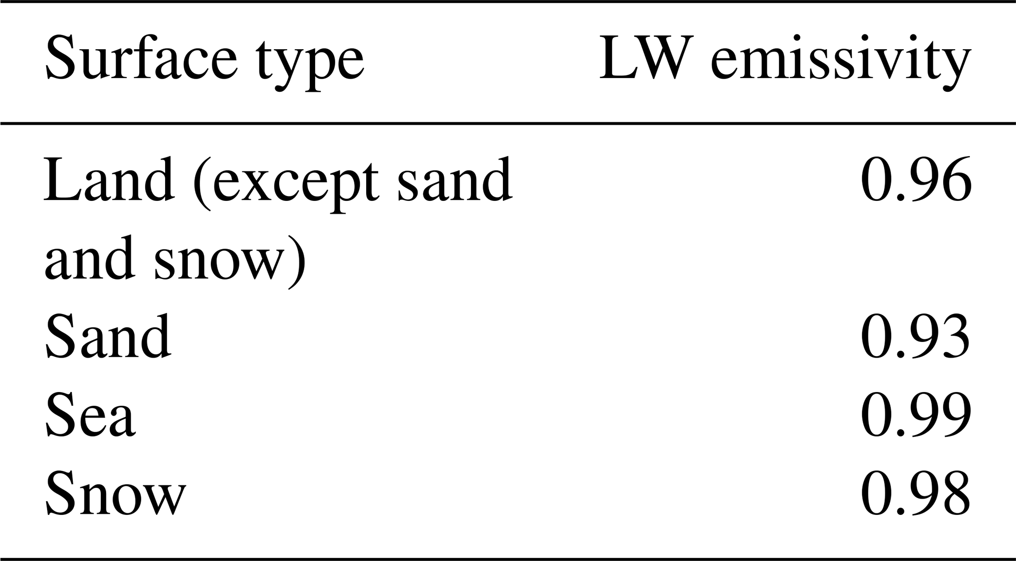
Table 2List of variables used by the offline radiative-transfer model ecRad and their provenance. All variables are set as daily averages.

The distributions taken from the CAMS reanalysis as inputs to the CAMS radiative-transfer calculations are listed in Table 2. The distributions are used as the mean of four time steps (00:00, 06:00, 12:00, and 18:00 Z) for the reanalysis dated 00:00 Z daily. The distributions are used at the degraded horizontal resolution of , down from the original resolution, to reduce computational cost. That decrease in resolution causes negligible (third decimal place) changes in globally averaged RF. Daily averaged concentrations of carbon dioxide and methane are taken from the data-assimilated, three-dimensional distributions obtained by CAMS Greenhouse Gases Fluxes (Chevallier et al., 2005; Bergamashi et al., 2013) for carbon dioxide and methane, respectively, with updates to both documented at https://atmosphere.copernicus.eu (last access: 14 July 2020). Nitrous oxide is set to its pre-industrial mixing ratio of 270 ppb (Myhre et al., 2013a). The inversion product versions used are v18r2 for carbon dioxide and v17r1 for methane. Figure 2 shows time series of global monthly total-column averages of carbon dioxide and methane concentrations. The annually averaged carbon dioxide concentration in 2017 was 404 ppm, up 8 % from 374 ppm in 2003. For methane, the concentration for year 2017 was 1804 ppb, up 4 % from 1730 ppb in 2003. Figure 2 also shows equivalent time series for background surface measurements by the NOAA Earth System Research Laboratory (downloaded from https://www.esrl.noaa.gov/gmd/ccgg/trends/global.html#global_data, last access: 14 July 2020) for carbon dioxide and by the Advanced Global Atmospheric Gases Experiment (AGAGE, downloaded from https://agage.mit.edu/data/agage-data, last access: 14 July 2020) for methane. Surface measurements are generally higher than the column averages, especially for methane that decreases with height by oxidation.

Figure 2Time series of globally and monthly averaged concentrations of (a) carbon dioxide (ppm) and (b) methane (ppb) over the period 2003–2017. Bold lines show mass-weighted total column averages for the CAMS Greenhouse Flux Inversion products. Thin lines show background surface measurements from NOAA's Earth System Research Laboratory for carbon dioxide and the Advanced Global Atmospheric Gases Experiment for methane, respectively.
Adjustment of radiative fluxes to account for changes in stratospheric temperatures uses the fixed dynamical heating (FDH) method (Ramaswamy et al., 2001). Convergence is reached when globally averaged changes in heating rate, RF, and stratospheric temperature become less than 0.05 K d−1, 0.05 W m−2, and 0.01 K, respectively. The maximum number of iterations is also set to 200. Once stratospheric adjustment is complete, the sum of the SW + LW radiative fluxes at the tropopause equals that at the top of the atmosphere. Methane RF is given in the LW and SW parts of the spectrum, although it is now known that ecRad – similar to many other radiative-transfer codes used in global models – is unlikely to properly handle methane absorption bands in the SW part of the spectrum because it does not have sufficient spectral resolution. Therefore, the CAMS products likely underestimate methane RF in the SW spectrum, and that underestimate affects its stratospheric adjustment. The SW contribution may be of the order of 15 % of total methane RF (Etminan et al., 2016).
2.2 Aerosol–radiation interactions
To obtain aerosol RF, it is necessary to distinguish between aerosols of natural origin and aerosols of anthropogenic origin. The ECMWF IFS does not keep track of the aerosol origin mainly to keep computational cost reasonable but also due to the following reasons.
-
Aerosol origin is not always given in emission inventories.
-
The same aerosol particle may be an internal mixture with anthropogenic and natural contributions.
-
Data assimilation cannot constrain natural and anthropogenic aerosols separately.
Instead, aerosol origin is obtained using the algorithm described by Bellouin et al. (2013), where aerosol size is used as a proxy for aerosol origin. The algorithm identifies four aerosol origins: anthropogenic, mineral dust, marine, and land-based fine-mode natural aerosol. The latter originates mostly from biogenic aerosols. The reader is referred to Sect. 3 of Bellouin et al. (2013) for details of the algorithm. The present paper describes two updates made to the algorithm since the publication of Bellouin et al. (2013).
The first update is the replacement of continental-wide anthropogenic fractions used over land surfaces by a fully gridded dataset that includes seasonal variations. Over land, identification of component aerosol optical depths (AODs) starts with removing the contribution of mineral dust aerosols from total AOD. The remaining non-dust AOD, τnon-dust, is then distributed between anthropogenic and fine-mode natural components, referred to as τanth and τfine-mode, respectively, as follows:
where fanth is the anthropogenic fraction of the non-dust AOD. In Bellouin et al. (2013), fanth was prescribed over broad regions on an annual basis. Here, fanth is given by monthly distributions on a grid. This new dataset derives from an analysis of AeroCom 2 numerical models (Kinne et al., 2013). Its annual average is shown in Fig. 3. Anthropogenic fractions show a north–south gradient, as expected from the location of population and industrial activities. Anthropogenic fractions are larger than 0.8 over most industrialised regions of North America, Europe, and Asia. The largest fractions are located over China, where more than 90 % of non-dust AOD is attributed to anthropogenic aerosols. In the Southern Hemisphere, anthropogenic fractions are typically smaller than 0.7 on an annual average. In terms of seasonality, anthropogenic fractions remain larger than 0.7 throughout the year in the Northern Hemisphere, with a peak in winter when energy consumption is high. In the Southern Hemisphere, seasonality is driven by biomass-burning aerosols, which are considered purely anthropogenic in the CAMS Climate Forcing estimates. Anthropogenic fractions therefore peak in late boreal summer in South America and southern Africa.
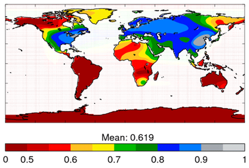
Figure 3Annually averaged anthropogenic fraction of non-dust aerosol optical depth over land at 0.55 µm.
The second change concerns the fine-mode fraction (FMF) of marine AOD at 0.55 µm, which gives the fraction of marine AOD that is exerted by marine particles with radii smaller than 0.5 µm. In Bellouin et al. (2013), this fraction was set to a fixed value of 0.3. Here, this fraction is determined by a gridded dataset that includes monthly variations. The dataset is obtained by applying the method of Yu et al. (2009) to daily MODIS Collection 6 aerosol retrievals of AOD and FMF. First, the marine aerosol background is isolated by selecting only ocean-based scenes where total AOD at 0.55 µm is between 0.03 and 0.10. Then, an AOD-weighted averaged FMF is computed. The analysis has been applied to retrievals from MODIS instruments on both the Terra (dataset covering 2001–2015) and Aqua (dataset covering 2003–2015) platforms. Both instruments yield very similar marine FMF distributions, and the distributions used here are the multi-annual monthly averages of the two instruments. Figure 4 shows the marine FMF derived from MODIS/Terra for the months of January and July. It suggests that marine FMF varies over a wide range of values. Regions of high wind speeds, around 40–50∘ in both hemispheres, are associated with large FMFs, indicating that the marine aerosol size distribution includes a sizable fraction of smaller particles there. There are indications of contamination by fine-mode anthropogenic and mineral dust aerosols in coastal areas, but the impact on speciated AODs is small because the aerosol identification algorithm uses broad FMF categories rather than absolute values. Indeed, anthropogenic AOD decreases only slightly in the roaring forties in the Southern Ocean and tends to increase slightly in the northern Atlantic and Pacific oceans. On a global average, the change in anthropogenic AOD due to the improved specification of marine FMF is +0.001 (+1.4 %). Bellouin et al. (2013) estimated the relative uncertainty in τanth at 18 %. The updates to land-based anthropogenic fractions and marine FMF described here are not expected to reduce their large contribution to that uncertainty.
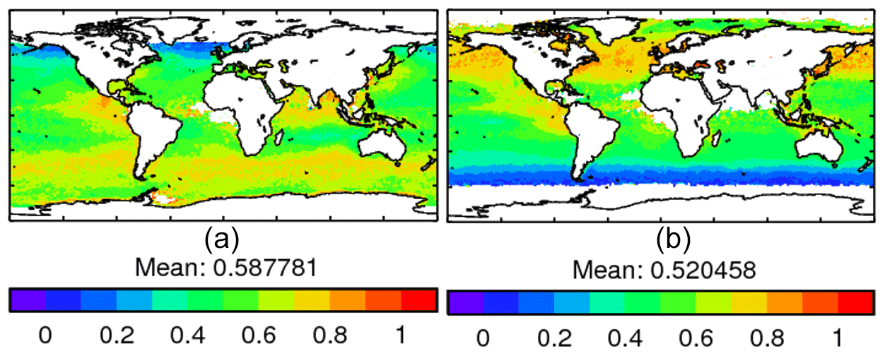
Figure 4Fine-mode fraction of marine aerosol optical depth at 0.55 µm as derived from MODIS/Terra Collection 6 aerosol retrievals for the months of January (a) and July (b).
Radiative effect and forcing of aerosol–radiation interactions are computed by radiative-transfer calculations that combine the speciated AODs derived above with prescriptions of aerosol size distribution and single-scattering albedo. The methods are as described in Sect. 4 of Bellouin et al. (2013) with one exception: the prescription of single-scattering albedo has been updated from a few continental-wide numbers to gridded monthly climatologies. This updated dataset introduces two major improvements compared to Bellouin et al. (2013). First, the new dataset provides the monthly cycle of fine-mode absorption. Second, the dataset is provided on a finer, grid. The method used to produce the dataset is described in Kinne et al. (2013). First, distributions of fine-mode extinction and absorption AODs are obtained from a selection of global aerosol numerical models that participated in the AeroCom simulations using a common set of aerosol and precursor emissions for present-day conditions (Kinne et al., 2006). To include an observational constraint, those modelled distributions are then merged with retrievals of aerosol single-scattering albedo (SSA) for the period 1996–2011 at more than 300 AERONET sites. The merging is based on a subjective assessment of the quality of the measurements at each of the AERONET sites used, along with their ability to represent aerosols in a wider region around the site location. The main impact of merging observed SSAs is to make aerosols in Africa and South Asia more absorbing than numerical models predicted. The distribution of annual and column-averaged aerosol SSA is shown in Fig. 5. The dataset represents the local maximum of absorption over California and the change in absorption as biomass-burning aerosols age during transport, which is visible over the south-eastern Atlantic. Over Asia, Europe, and South America, absorption is also larger near source regions, with less absorption elsewhere.

Figure 5Annually averaged distribution of column-averaged single-scattering albedo at 0.55 µm used to characterise absorption of anthropogenic aerosols.
It is worth noting that the SSA distribution characterises absorption of fine-mode aerosols but is used to provide the absorption of anthropogenic aerosols, which is not fully consistent. The inconsistency is, however, mitigated by two factors. First, fine-mode aerosols are the main proxy for anthropogenic aerosols in the Bellouin et al. (2013) algorithm that identifies aerosol origin, and their distributions are broadly similar. Second, regions where natural aerosols such as marine and mineral dust may contaminate the fine-mode AOD often correspond to minima in anthropogenic AOD.
Like in Bellouin et al. (2013), the RF of aerosol–radiation interactions (RFari) is estimated in clear-sky (cloud-free sky) then scaled by the complement of the cloud fraction in each grid box to represent all-sky conditions, thus assuming that cloudy-sky aerosol–radiation interactions are zero. Experimental estimates of cloudy-sky RF have been done but are based on a simplified account of cloud albedo, which limits their usefulness. For the year 2003, globally averaged above-cloud anthropogenic and mineral dust AODs weighted by cloud fraction are 0.005 and 0.003, respectively, or 8 % of their clear-sky counterparts. Above-cloud marine and fine-mode natural AODs are negligible. Above-cloud anthropogenic aerosols exert a positive radiative effect because of their absorbing nature and the high reflectance of clouds. Those radiative effects commonly reach +5 to +10 W m−2 locally during the biomass-burning season that lasts from late August to October over the south-eastern Atlantic stratocumulus deck. However, this only translates into a cloudy-sky anthropogenic RFari of +0.01 W m−2, in agreement with AeroCom-based estimates, which span the range W m−2 (Myhre et al., 2019). Studies based on the Cloud-Aerosol Lidar with Orthogonal Polarization (CALIOP) estimate that all-sky radiative effects of present-day above-cloud aerosols range between 0.1 and 0.7 W m−2 on an annual average over 60∘ S to 60∘ N (Oikawa et al., 2018; Kacenelenbogen et al., 2019), but only a fraction of that radiative effect contributes to RFari because of compensations from pre-industrial biomass-burning aerosols. Neglecting above-cloud aerosols therefore introduces a small uncertainty into the global average but leads to larger errors regionally and seasonally.
2.3 Aerosol–cloud interactions
The algorithm that estimates the RF of aerosol–cloud interactions (RFaci) is the same as that used in Bellouin et al. (2013). It is based on satellite-derived cloud susceptibilities to aerosol changes, which are given seasonally and regionally. Statistics of satellite retrievals of liquid clouds are poor at high latitudes (Grosvenor et al., 2018), so cloud susceptibilities are not available poleward of 60∘ and RFaci is not estimated there. Aerosol changes are obtained by the anthropogenic AOD derived in Sect. 2.2. The cloud susceptibilities are applied to low-level (warm) clouds only.
3.1 Carbon dioxide and methane
The three-dimensional distributions of carbon dioxide and methane derived for present-day (PD) strongly benefit from data assimilation of surface measurements and satellite retrievals, which partly offset the biases of the chemistry model. That, however, creates the difficulty that estimating PI concentrations by running the chemistry model with PI emissions would be biased with respect to the data-assimilated, present-day distributions. Instead, daily PI mixing ratios of carbon dioxide and methane are scaled from daily CAMS Greenhouse Gas Flux mixing ratios in each grid box and at each model level using the following equation:
where [X] denotes the mixing ratio of carbon dioxide or methane, and angle brackets denote annual averaging. All variables are taken from the CAMS Greenhouse Gas Flux inversions, except for PI surface mixing ratios, , which come from footnote a of Table 8.2 of Myhre et al. (2013a), 278 ppm for carbon dioxide and 772 ppb for methane. The scaling factors are calculated at the surface because this is the level where PI concentrations are given in Myhre et al. (2013a): the whole profile is scaled like the surface level, which is justified by the relatively well-mixed nature of both gases. By construction, the scaled PI distribution has the same global, annual average value at the surface as given in Myhre et al. (2013a) but inherits the horizontal, vertical, and temporal variabilities of the PD distribution. Using this scaling method replicates the PD amplitude of the seasonal cycle of carbon dioxide and methane concentrations. For carbon dioxide, there is a suggestion from modelling studies that the amplitude of the seasonal cycle may have increased since PI (Lindsay et al., 2014). Replicating the PD amplitude would therefore cause a small underestimate of the forcing.
3.2 Ozone
Like carbon dioxide and methane, ozone distributions in the CAMS reanalysis are strongly affected by data assimilation of ozone profiles and total and partial columns (Inness et al., 2015). Consequently, it is also not advisable to simply simulate PI ozone concentrations by running the chemistry model with PI emissions, as that would introduce biases between a data-assimilated PD and a free-running PI. Instead, daily PI ozone mixing ratios are scaled in each grid box and at each model level from daily CAMS reanalysis mixing ratios as follows:
where [O3] denotes ozone mixing ratios and angle brackets denote monthly averaging. and are taken from the three-dimensional CMIP6 input4MIPs ozone concentration dataset of Hegglin et al. (2016), briefly described by Checa-Garcia et al. (2018), for the years 2008–2012 for PD and 1850–1899 for PI. The Hegglin et al. (2016) dataset was obtained by merging 10-year running-averaged simulated ozone distributions by the Canadian Middle Atmosphere Model (CMAM) and the Whole Atmosphere Chemistry Climate Model (WACCM), both driven by CMIP5 historical emissions (Lamarque et al., 2010). The models resolve the chemistry and dynamics of the troposphere and stratosphere, allowing for mutual influence. Historical stratospheric ozone reflects the effects of long-lived greenhouse gases such as carbon dioxide, nitrous oxide, and methane in a physically and chemically consistent way. The interannual variability, including the Quasi-Biennial Oscillation, is included. The CMAM pre-industrial control configuration uses precursor and greenhouse gas emissions for the year 1850 in a 40-year simulation, with the last 10 years used to create the mean ozone field. The WACCM pre-industrial control configuration averages precursor and greenhouse gas emissions over the 1850–1859 period. The reference spectral and total irradiances are derived from averages over the period 1834–1867 (solar cycles 8–10), but the 11-year solar cycle is not considered.
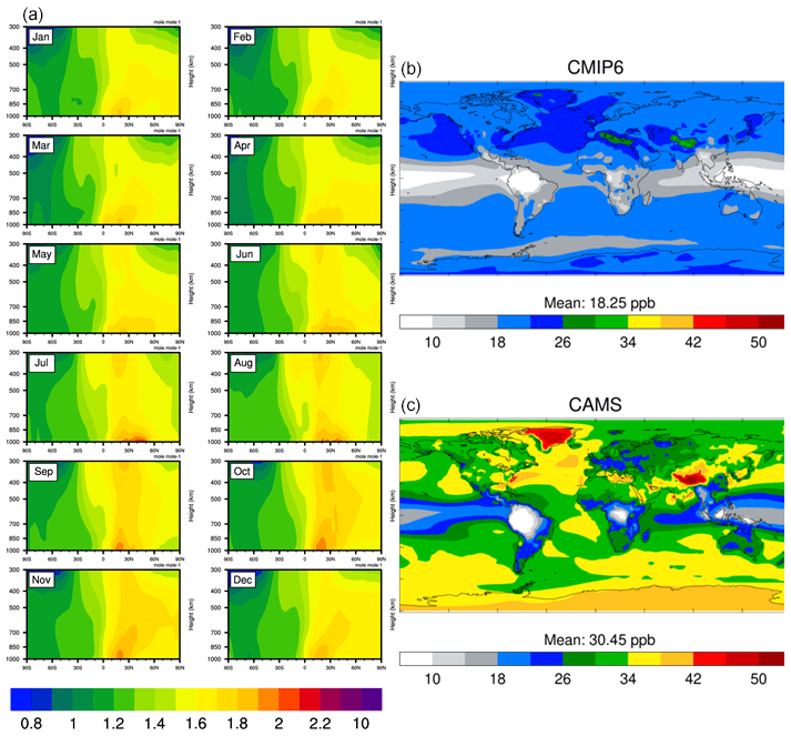
Figure 6(a) Monthly averaged zonal cross sections of ratios of present-day (2008–2014) to pre-industrial (1850–1900) ozone mass-mixing ratios from the CMIP6 input4MIPs climatology. Surface ozone volume mixing ratios (in ppb) in (b) the CMIP6 input4MIPs climatology and (c) scaled from the CAMS reanalysis using the ratios shown on the left.
Figure 6 shows the monthly cross sections of the PD-to-PI ratios used to scale CAMS reanalysis ozone mixing ratios following the equation above. The ratios exhibit a strong hemispheric contrast. In the Northern Hemisphere, ratios are typically larger than 1.5 throughout the year and can be around 2 in the lower troposphere above polluted regions. In the Southern Hemisphere, ratios are closer to 1.2 and are below 1 in the upper tropospheric Antarctic ozone hole, where the ozone layer has been diminished since PI conditions. Figure 6 also compares surface ozone volume mixing ratios in the Hegglin et al. (2016) dataset for the year 1850 to those resulting from scaling CAMS reanalysis ozone concentrations, averaged over the period 2003–2016. CAMS PI surface ozone is about 1.7 larger than in the Hegglin et al. (2016) dataset. The global distribution of PI ozone concentrations is poorly known due to a lack of measurements in different regions of the world, but ACCMIP models (Young et al., 2013) and the isotopic analysis of Yeung et al. (2019) suggest that the PI ozone levels in the Northern Hemisphere were of the order of 20 to 30 ppbv in the Northern Hemisphere and 10 to 25 ppbv in the Southern Hemisphere. CAMS estimates are higher, probably because of overestimations of surface ozone in the CAMS reanalysis, especially in the Tropics and Northern Hemisphere (Inness et al., 2019), which propagate to the PI estimates. Although it will be good to reduce those biases in future versions of the dataset, the fact that both PI and PD ozone concentrations are similarly biased should not have a large impact on tropospheric ozone RF, which mostly depends on the PI to PD increment in ozone concentrations.
3.3 Aerosols
The anthropogenic AOD (Sect. 2.2), which is then used to estimate RFari and RFaci, is defined with respect to PD natural aerosols, which is a different reference to PI (1750) so a correction is required (Bellouin et al., 2008). That correction factor is taken from Bellouin et al. (2013) and is equal to 0.8; i.e. RFari and RFaci defined with respect to PI are 80 % of RFari and RFaci defined with respect to PD natural aerosols.
Model uncertainty can be structural or parametric in nature. The structural uncertainty relates to methodological and parameterisation choices in the characterisation of the radiative forcing. It is known to be influenced by the atmospheric time step used in evaluating the radiative forcing (Colman et al., 2001), the effect of any climatological averaging (Mülmenstädt et al., 2019) and for IRF or RF, the definition of tropopause (Collins et al., 2006). Parametric uncertainty relates to choices of the value of the parameters within the parameterisations. As radiation calls are expensive, in climate reanalysis or general circulation models the SW and LW parts of the spectrum are divided into a small number of bands that exhibit similar scattering and absorption properties. This parameterisation error can be significant (Collins et al., 2006; Pincus et al., 2015). Different radiative-transfer solvers divide the bands in different ways, and the choice of radiative-transfer code contributes structural uncertainty (as there are methodological differences in how the radiative-transfer equation is solved) in addition to parametric uncertainty. Parametric uncertainty is also present from the choices of which refractive index to use for calculating aerosol scattering and absorption processes.
4.1 Uncertainty from methodological choices
All experiments in this section are performed using the CAMS reanalysis dataset for the year 2003. Greenhouse gas concentrations for carbon dioxide, methane, and nitrous oxide but also for CFC-11, CFC-12, HCFC-22, and CCl4 from 2003 and 1850 are taken from the Representative Concentration Pathways (RCP) historical dataset (Meinshausen et al., 2011). Although these forcings do not comprise the totality of anthropogenic greenhouse gas RF, 98 % of the well-mixed greenhouse gas RF is included from these species according to Table 8.2 of Myhre et al. (2013a), which is for the year 2011.
4.1.1 Time stepping and averaging
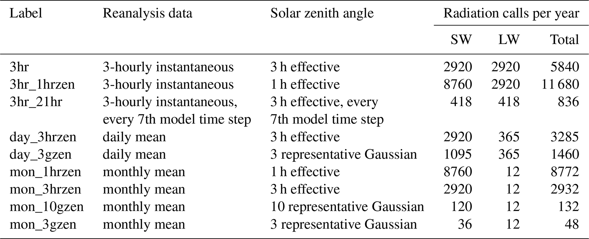
Uncertainty relating to time stepping comes from both the resolution of the climatology (the effect of averaging or sampling frequency of the input data), as well as the frequency of the radiation calls. Table 3 summarises the nine time-stepping and climatological-averaging experiments undertaken to quantify that uncertainty. In the IFS, full radiation calls are only made every 3 simulated hours, with reduced radiation calls made on intermediate model time steps (30 min), to mitigate against the high cost of radiative-transfer calculations. Alongside using 3 h instantaneous data, reanalysis data are prepared as both daily and monthly means with a range of reduced-frequency radiation call methodologies. In the SW this requires an appropriate choice of solar zenith angle. Alongside the standard case of 6 representative solar zenith angles per day, we investigate 6 and 20 representative zenith angles for monthly averaged climatologies. The impact of averaged climatologies is also isolated by using 3 h solar zenith angles with daily and monthly climatologies. In addition, an experiment using instantaneous 3-hourly reanalysis in which we retain every seventh model output time step (i.e. interval of 21 h) is performed. This experiment does not introduce bias from averaging the underlying reanalysis data while reducing the number of radiation calls. A 21 h sampling frequency is chosen to preserve the diurnal and seasonal insolation cycles, as recommended in partial radiative perturbation studies (Colman et al., 2001). The approximations introduced by using a 3-hourly effective zenith angle are compared by using the same underlying reanalysis data with a 1-hourly effective zenith angle. At periods of 1 h or less, the effective and instantaneous zenith angles are very similar in most grid points.
Table 3Time-stepping and climatological-averaging experiments.
Top-of-atmosphere flux imbalance
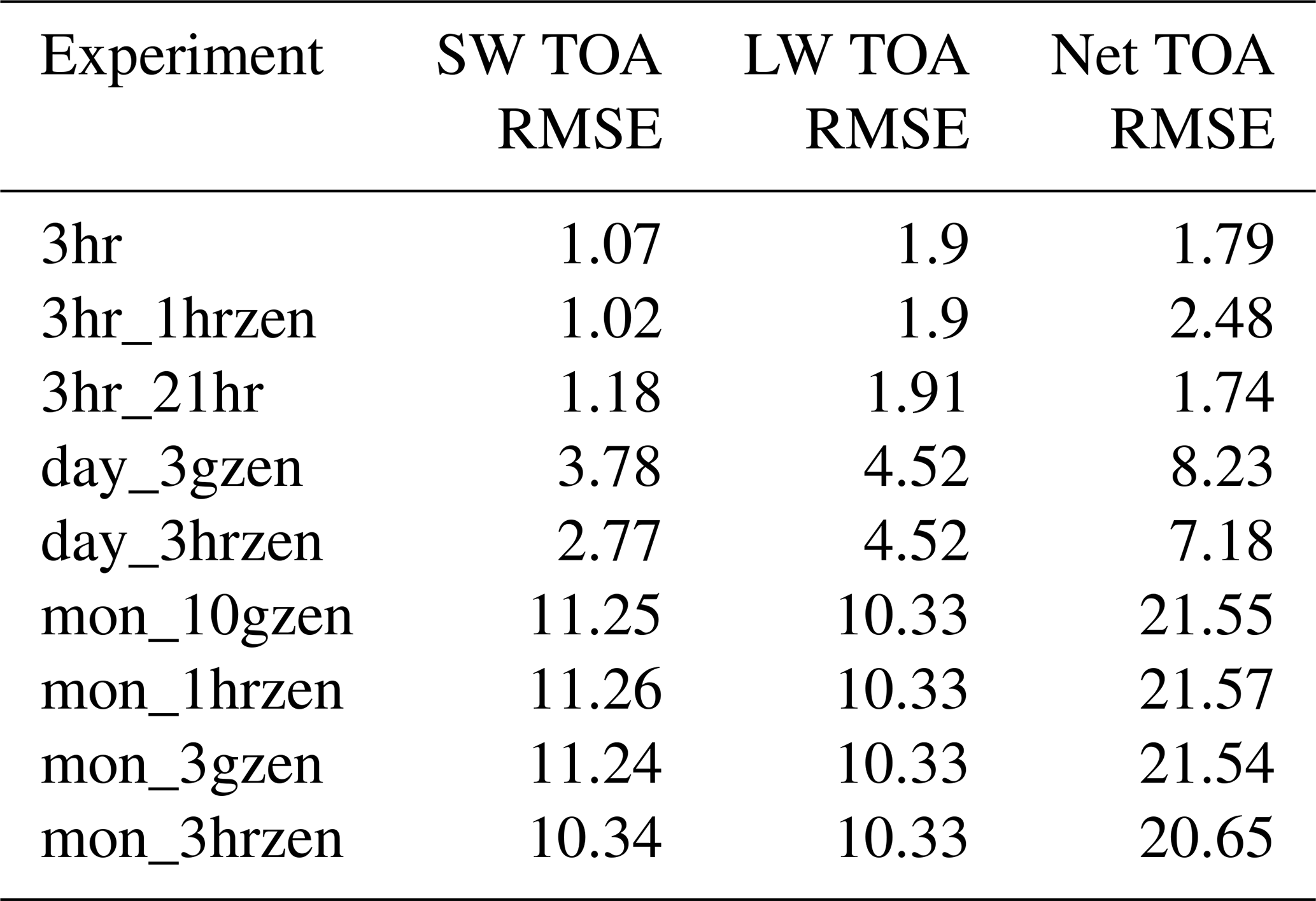
Although the focus of this work is the accuracy of the RF, it is useful to explore the dependency of the present-day simulation of TOA irradiances on the time-stepping. Figure 7 shows the results from the time-stepping experiment, and root-mean-squared errors (RMSEs) for the simulated data versus observations from the Clouds and the Earth's Radiant Energy System, Energy Balanced and Filled dataset (CERES EBAF TOA Ed4.0) (Loeb et al., 2018) are given in Table 4. The CERES data assumes a nominal TOA height of 20 km, which is well above the cloud layer, so radiative fluxes are not significantly different to those at the top level of the model. Figure 7a shows that accuracy in the SW upwelling TOA radiation is compromised by using climatological averaging. Monthly averaging is 3 to 4 times less accurate than daily averaging, whereas 3-hourly instantaneous climatologies agree well with observations. This result agrees with Mülmentstädt et al. (2019). Figure 7b shows the corresponding fluxes for LW outgoing radiation. Again, 3-hourly instantaneous climatologies perform better than daily, which in turn perform better than monthly. Agreement with observations is less good with the 3-hourly instantaneous radiative fluxes in the LW than in the SW. Figure 7c shows net TOA radiation. Again, 3 h instantaneous climatologies agree better with observations than daily means, which are in turn better than monthly means. Biases with mean climatologies add rather than cancel, as upwelling radiation is underestimated in both the LW and the SW for daily and monthly means. Note that Fig. 7 and Table 4 suggest that the effect of climatological averaging dominates over the frequency of SW radiation calls.
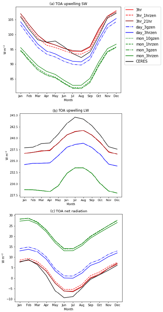
Figure 7Radiative fluxes calculated by ecRad using 2003 CAMS reanalysis data for the nine time-stepping experiments described in Table 3 (coloured lines): (a) top-of-atmosphere shortwave upwelling radiative flux, (b) top-of-atmosphere longwave upwelling radiative flux, (c) top-of-atmosphere net downwelling radiation. The black line shows the observed radiation fluxes for CERES EBAF.
Table 4Root-mean-square error (RMSE, in W m−2) of monthly top-of-atmosphere (TOA) radiation compared to CERES-EBAF for 2003.
Radiative forcing at top-of-atmosphere and tropopause
Here, IRF is estimated by comparing all-sky net fluxes at the tropopause and at the TOA for 2003 and 1850. A simplified definition of the tropopause is employed for this comparison, defined as the 29th model level in the CAMS reanalysis, the level closest to 200 hPa. Alternative tropopause assumptions are investigated below. For the purpose of these experiments, the 1850 atmosphere is created by adjusting the concentrations of the eight greenhouse gases included in the ecRad code to 1850 levels following Meinshausen et al. (2011). Mixing ratios of ozone and aerosol species are prescribed using a gridded PI to PD ratio. Meteorology (temperature, water vapour, and cloud variables) is fixed at 2003 levels in all experiments.
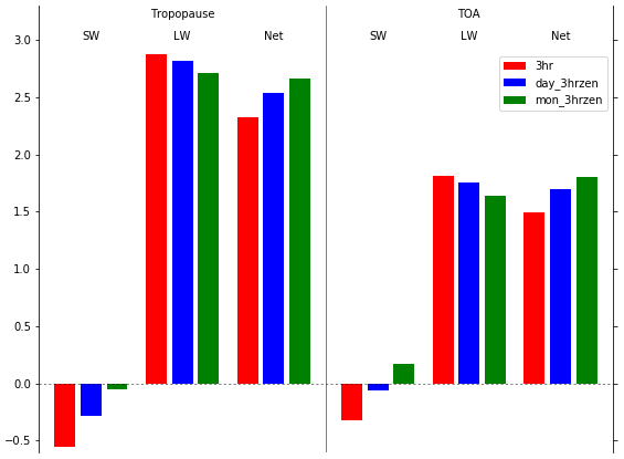
Figure 8Global-mean instantaneous radiative forcing for the year 2003 (in W m−2) at the tropopause and top of atmosphere for 3-hourly solar zenith angle time steps for 3-hourly, daily, and monthly climatologies.
Figure 8 shows the results for the 3hr, day_3hrzen and mon_3hrzen experiments. In the absence of PI observations, the RF calculated in the 3hr experiment is assumed to be closest to the truth, given the better agreement to CERES TOA fluxes than the daily or monthly averaged reanalysis data. Corresponding time-stepping experiments for different solar zenith time steps give almost identical results. SW IRF is deficient when using averaged climatology, with TOA mon_3hrzen disagreeing in sign with 3hr. The errors introduced in the LW by climatological averaging are relatively small, amounting to about 6 % at the tropopause and 10 % at the TOA for mon_3hrzen compared to 3hr. Although LW forcing dominates, the errors in the SW forcing are of larger magnitude, so the net climatological averaging effect is 15 % at the tropopause and 21 % at the TOA. The error in net IRF is 0.21 W m−2 at the tropopause for day_3hrzen (and day_3gzen, not shown) compared to 3hr. This is used as our uncertainty range in the CAMS reanalysis RF product, which is calculated using a day_3gzen methodology.
4.1.2 Spatial resolution of reanalysis data
To determine whether the grid resolution for RF calculation introduces additional error, the 2003 TOA fluxes were analysed using the 3hr_21hr methodology at the native model resolution of . Only minor differences are found in the TOA radiative fluxes: −0.02 W m−2 in the SW and +0.07 W m−2 in the LW, resulting in a +0.05 W m−2 net difference. As the pre-industrial ratios of ozone and aerosol precursors are not available on this higher-resolution grid, IRF cannot be calculated using the finer grid, but IRF errors are likely to be even smaller because taking the difference in TOA (or tropopause) fluxes is expected to result in smaller errors than the absolute TOA difference. The spatial resolution error is assessed to be 0.05 W m−2.
4.1.3 Tropopause definition
Figure 8 shows that TOA IRF differs significantly from tropopause IRF – in fact the difference, which is mostly due to carbon dioxide, explains the need for stratospheric temperature adjustment. But regardless of whether IRF or RF is estimated, there is a need to define the tropopause and quantify the impact of that definition on estimated RF (Forster and Shine, 1997). The uncertainty analysis is done on tropopause IRF because of the large number of radiation calls needed to produce an FDH estimate of RF. Experiment 3hr_21hr is used as a basis to investigate the uncertainty in the tropopause definition for IRF.
The default definition of the tropopause used in CAMS RF estimates is the WMO definition of the lowest altitude at which lapse rate drops to 2 K km−1, providing the lapse rate in the 2 km above this level does not exceed 2 K km−1. The tropopause level is calculated daily. Alternative definitions used here are as follows:
-
the 200 hPa level, calculated by interpolating ecRad-calculated fluxes on model levels in logarithm of pressure, this level is used as a proxy for the tropopause from model results in the RF inter-comparison of Collins et al. (2006);
-
level 29 of the CAMS reanalysis grid, which is closest to 200 hPa at most locations and easy to obtain;
-
a linearly varying tropopause, from 100 hPa at the Equator to 300 hPa at the poles, as used by Soden et al. (2008);
-
100 hPa from the Equator to 39∘ N/S, where it drops abruptly to 189 hPa and is then linear in latitude to 300 hPa at the poles, as used by Hansen et al. (1997);
-
the CAMS model-defined tropopause but calculated from instantaneous 3 h fields instead of daily.
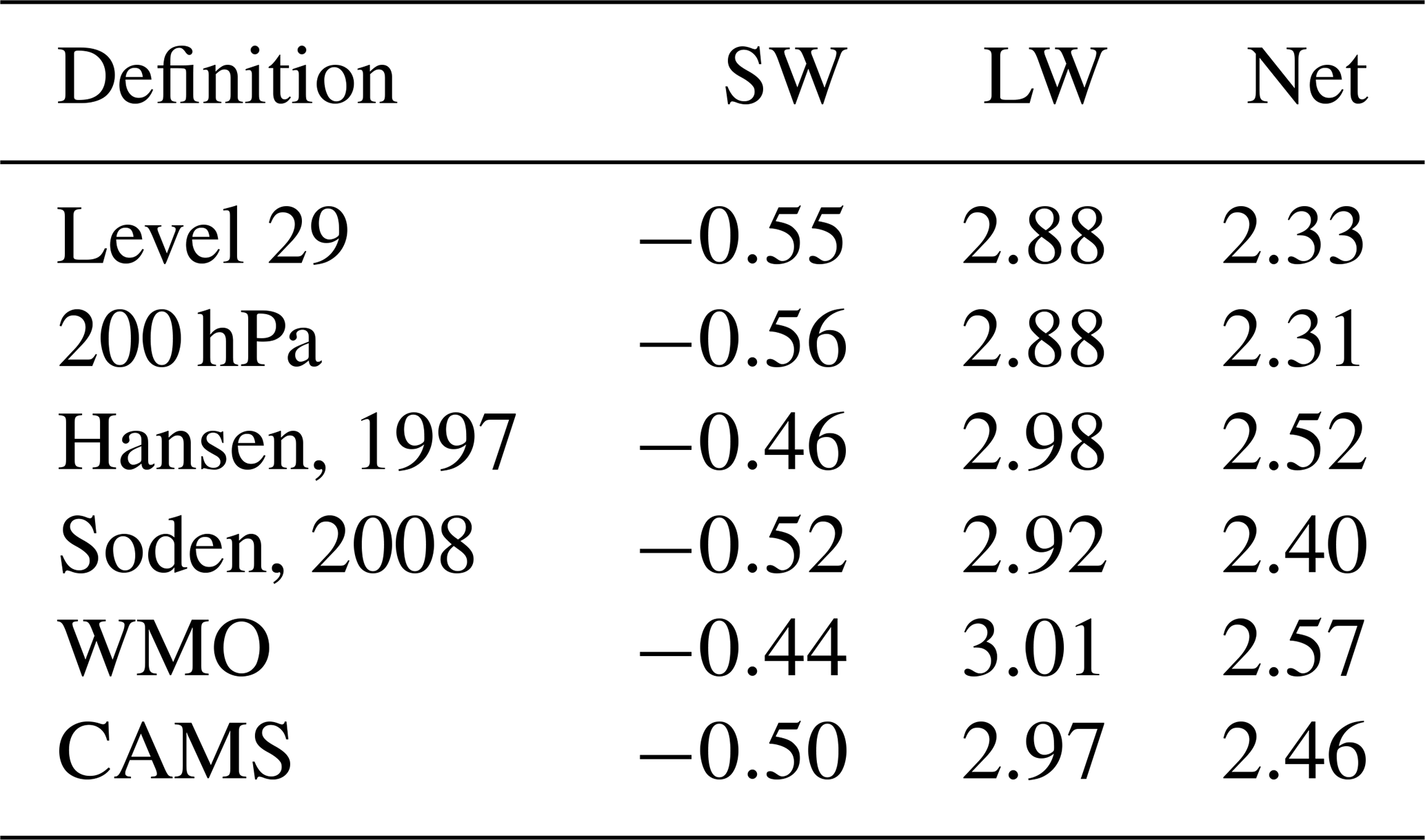
Results are presented in Table 5. The WMO definition gives the largest net IRF at 2.57 W m−2 at the tropopause, whereas the CAMS definition of the tropopause results in a net IRF of 2.46 W m−2, giving a difference of 5 %. In determining the tropopause level uncertainty, equal weight is assigned to the WMO, CAMS, Soden et al. (2008), and Hansen et al. (1997) definitions. A weighting of 0.5 is assigned to the level 29 and 200 hPa definitions, as they are measuring the same quantity. The CAMS and WMO definitions are considered sufficiently different to be treated as independent. Using these weights, the uncertainty for the choice of tropopause level is assessed as 0.15 W m−2, which is the 5 % to 95 % confidence interval of the estimates taking into account weighting.
Table 5Shortwave, longwave, and net instantaneous radiative forcings (in W m−2) calculated with different tropopause definitions.
4.1.4 Radiative-transfer code
Structural uncertainty is introduced by the reduction of both the solar and thermal radiation into a small number of spectral bands. This reduction is required to facilitate rapid run time of radiation schemes in GCM and reanalysis schemes, as radiative-transfer codes with higher spectral resolution are too computationally expensive. Structural uncertainty also arises from the choices of approximations and numerical methods used in the actual solving of the radiative-transfer equation. Parameterisation uncertainty arises from the treatment of scattering and absorption of gases, clouds, and aerosols. Further uncertainty is introduced by use of a two-stream radiative-transfer model, which is standard in most GCMs, as well as in ecRad, again for reasons of efficiency. This component of uncertainty is not quantified here, but, in the case of RFari, Randles et al. (2013) found biases of both signs due to two-stream models, depending on aerosol single-scattering albedo and solar zenith angle. They also noted that compensation of errors and the mitigating effect of delta scaling reduce two-stream biases of globally and annually averaged RFari compared to regional and seasonal estimates.
IRF calculated by ecRad is compared against the Suite Of Community Radiative Transfer codes based on Edwards and Slingo (SOCRATES), as configured in the UK Met Office's GA3.1 configuration (Manners et al., 2017) optimised for use in the HadGEM3 family of GCMs. In this configuration, SOCRATES uses a Delta-Eddington two-stream solver with 6 SW and 9 LW radiation bands. In comparison, ecRad uses 16 bands in the LW and 14 in the SW. Owing to the differences in how aerosols are specified between the ecRad and SOCRATES interfaces, comparisons are performed in aerosol-free cases. Aerosols may contribute further uncertainties, although Zhang et al. (2020) only found a small dependence of aerosol radiative effects on the spectral resolution of radiative-transfer calculations. All-sky and clear-sky cases are compared between ecRad and SOCRATES, but it should also be noted that methodological differences between the two codes, including the scattering and absorption profiles of cloud droplets and treatment of cloud overlap, may preclude a direct comparison of all-sky cases.
For the IRF calculations, full-year 3hr_21hr calculations with 2003 CAMS reanalysis are again used but with GHGs set to 1850 levels in the 1850 simulation. The simulations are run only with the greenhouse gases common to both codes (CO2, CH4, N2O, CFC11, CFC12, and HCFC22). A global effective radius of 10 µm is set for liquid water cloud droplets and 50 µm for ice crystals. The net GHG-only tropopause (level 29) IRF is 2.71 W m−2 in ecRad and 2.97 W m−2 in SOCRATES, whereas clear-sky IRF is 3.17 W m−2 in ecRad and 3.44 W m−2 in SOCRATES. SOCRATES therefore calculates a stronger IRF by about 10 %, which is not reduced by the inclusion of clouds.
One further comparison against a narrow-band calculation in the libRadtran implementation of DISORT (Mayer and Kylling, 2005) is performed for a global reference profile using the Representative Wavelength parameterisation (REPTRAN; Gasteiger et al., 2014) with a spectral resolution of 15 cm−1. The reanalysis data from 21 March 2003 at 15:00 Z is selected for clear-sky conditions only.
This comparison against the reference profile results in an IRF of 2.85 W m−2 in libRadtran, 3.13 W m−2 in ecRad and 3.34 W m−2 in SOCRATES. The error due to radiation parameterisation is estimated to be 0.33 W m−2 at the 5 % to 95 % level from these three estimates. The radiation code inter-comparison planned by the Radiative Forcing Model Intercomparison Project (RFMIP; Pincus et al., 2016) will further quantify uncertainties in GCM radiation codes.
4.2 Uncertainty from aerosol optical properties and climatology
In addition to the parametric uncertainty discussed in Sect. 4.1, there is parametric uncertainty from the base climate state unrelated to any climatological averaging. Meteorological reanalysis is not perfect since limited and spatially incomplete observations are used to drive an atmospheric model (Dee et al., 2011). Additionally, the SW, and to a lesser extent LW, transmission and reflectivity of the atmosphere is heavily dependent on aerosol optical properties, which are not well constrained from observations (Regayre et al., 2018; Johnson et al., 2018).
To quantify those uncertainties, a 240-member perturbed parameter ensemble (PPE) is built by sampling uncertainty in 24 input variables, including aerosol and greenhouse gas emission and composition parameters, using a Latin hypercube approach (Lee et al., 2011) according to assumed prior distributions (Table 6). For each sample set, a pair of 2003 and 1850 simulations is performed, using the 2003 reanalysis data as before. Prior distributions of each parameter are informed from literature ranges and other modelling studies. In many cases the prior distributions in Table 6 differ from those used in referenced studies. Our prior distributions are informed by the references but are adapted to account for known information about the default parameter combinations used in ecRad, which produce a 2003 IRF estimate that is well within the expected range (see Sect. 4.1.1). For example, the geometric standard deviation of the sulfate size distribution is modified from the prior used in Lee at al. (2013) of 1.2–1.8 to account for the fact that the IFS by default uses a relatively small size distribution mean radius of 35 nm with a larger geometric standard deviation of 2.0 than used in Lee et al. (2013). The prior for mean sulfate size distribution used in the PPE admits values that are mostly larger than 35 nm, so the geometric standard deviation is reduced to compensate.
Table 6Variables perturbed and their ranges for use in the 240-member perturbed parameter ensemble.
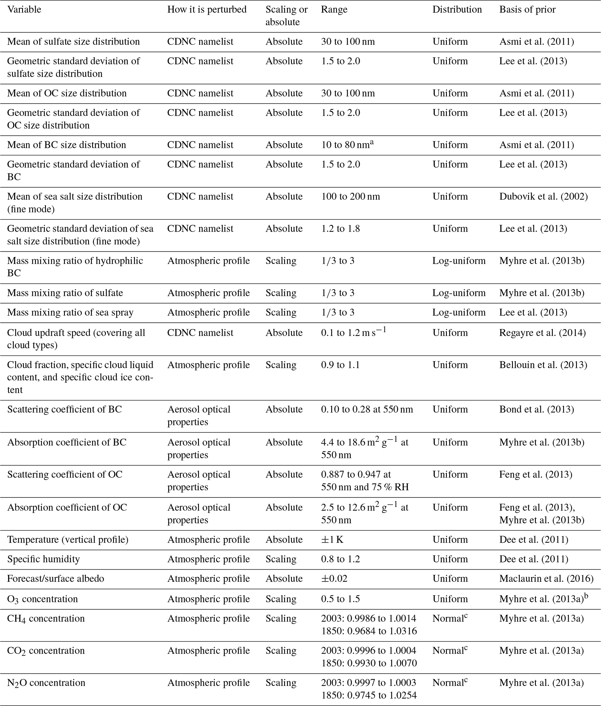
a Assumed to be lower than OC. b O3 forcing presumed to scale linearly with O3 concentration. c CH4, CO2, and N2O use the same relative uncertainty compared
to the
best-estimate concentrations for 1850 and 2003 simulations.
In this section, tropopause IRF is calculated on level 29, and a 3hr_21hr time-stepping methodology is used. The distribution of the global mean tropopause IRF for the year 2003 in the 240-member PPE using ecRad is shown in Fig. 9. The distribution of RF is positively skewed and well-represented by a lognormal distribution (red curve in Fig. 9). This contrasts with the anthropogenic forcing assessment in the IPCC AR5, which shows a mild negative skew (Myhre et al., 2013a), mostly due to the influence of the asymmetric uncertainty in AR5-assessed aerosol forcing. It should be noted, however, that the two different methods of arriving at distributions of radiative forcing are not equivalent and have different approaches to quantify sources of uncertainty.
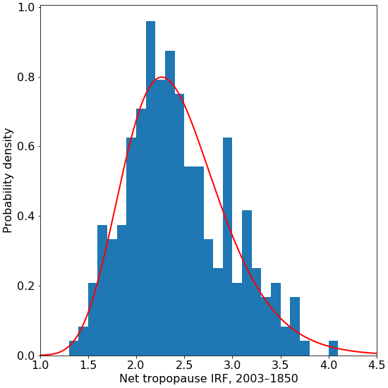
Figure 9Probability density function for the global annual mean instantaneous radiative forcing (W m−2) for the year 2003, resulting from the CAMS Climate Forcing Perturbed Parameter Ensemble. A lognormal fit to the distribution is shown in red.
The mean (5 %–95 %) IRF from the 240-member ensemble is 2.44 (1.67 to 3.42) W m−2, which is slightly stronger than the 2.33 W m−2 arising from using default ecRad parameters (Sect. 4.1.1). The mean (5 %–95 %) IRF from the lognormal curve fit is 2.44 (1.67 to 3.40) W m−2. Due to the good agreement between the sample and distribution fit, the mean and uncertainty range from the lognormal curve fit to the PPE are used in our overall uncertainty assessment for computational ease.
4.3 Combined uncertainty
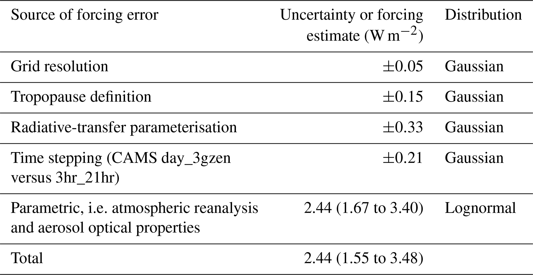
The individual sources of uncertainty from Sect. 4.1 and 4.2 are combined to produce an overall uncertainty estimate (Table 7). To produce the combined uncertainty, each individual source of uncertainty is assumed to be uncorrelated with the others. A million Monte Carlo samples were drawn from each distribution, corresponding to the individual sources of uncertainty listed in Table 7. This approach is taken as it is not straightforward to add non-symmetric uncertainties in quadrature. The combined uncertainty in IRF represents a range of 64 % to 143 % of the mean. This range is used to evaluate the RF uncertainty of the CAMS RF estimates, assuming that the uncertainty range calculated for the IRF in 2003 applies to all years.
Table 7Combined parametric and structural uncertainty in net tropopause instantaneous radiative forcing for 2003.
5.1 Overview
Figure 10 shows RF time series and average distributions over the CAMS reanalysis period 2003–2017. Over that period, RF of carbon dioxide and methane have increased by 26 % and 6 %, respectively, because their atmospheric concentrations have increased. Ozone and aerosol radiative forcing do not show significant trends over the period. In terms of distributions, carbon dioxide and methane RF peak in the Tropics and have a good degree of symmetry between the two hemispheres. Tropospheric ozone RF is also maximum in the Tropics but is larger in the Northern Hemisphere, where tropospheric pollution is larger, than in the Southern Hemisphere. Stratospheric ozone RF peaks at high latitudes. It is positive in the high latitudes of the Northern Hemisphere because of influences from the troposphere (see Sect. 5.3) and negative in the high latitudes of the Southern Hemisphere because of stratospheric ozone depletion, in good agreement with Checa-Garcia et al. (2018). RFari follows the distribution of anthropogenic aerosols, which are located over and downwind of polluted and wildfire regions. RFari is negative over most of the globe, except small areas of high-albedo desert regions where anthropogenic absorption switches the sign to positive. Recall that above-cloud RFari is neglected in those calculations, so areas of positive RF from biomass-burning aerosols overlying clouds (e.g. Zuidema et al., 2016) are not represented. RFaci is also heterogeneously distributed, with large RF exerted by aerosol perturbations to mid-latitude Northern Hemisphere clouds and stratocumulus decks.
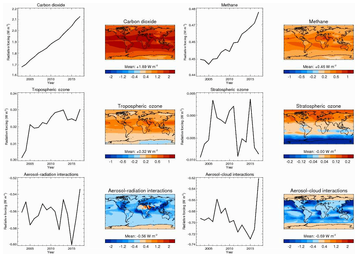
Figure 10Annual and global-mean time series and average distribution for the CAMS reanalysis period 2003–2017 of the stratospherically adjusted radiative forcing (relative to 1750 in W m−2) of carbon dioxide, methane, tropospheric ozone, stratospheric ozone, aerosol–radiation interactions, and aerosol–cloud interactions. Radiative forcing is given for shortwave plus longwave, except for aerosols where it is given for shortwave only.
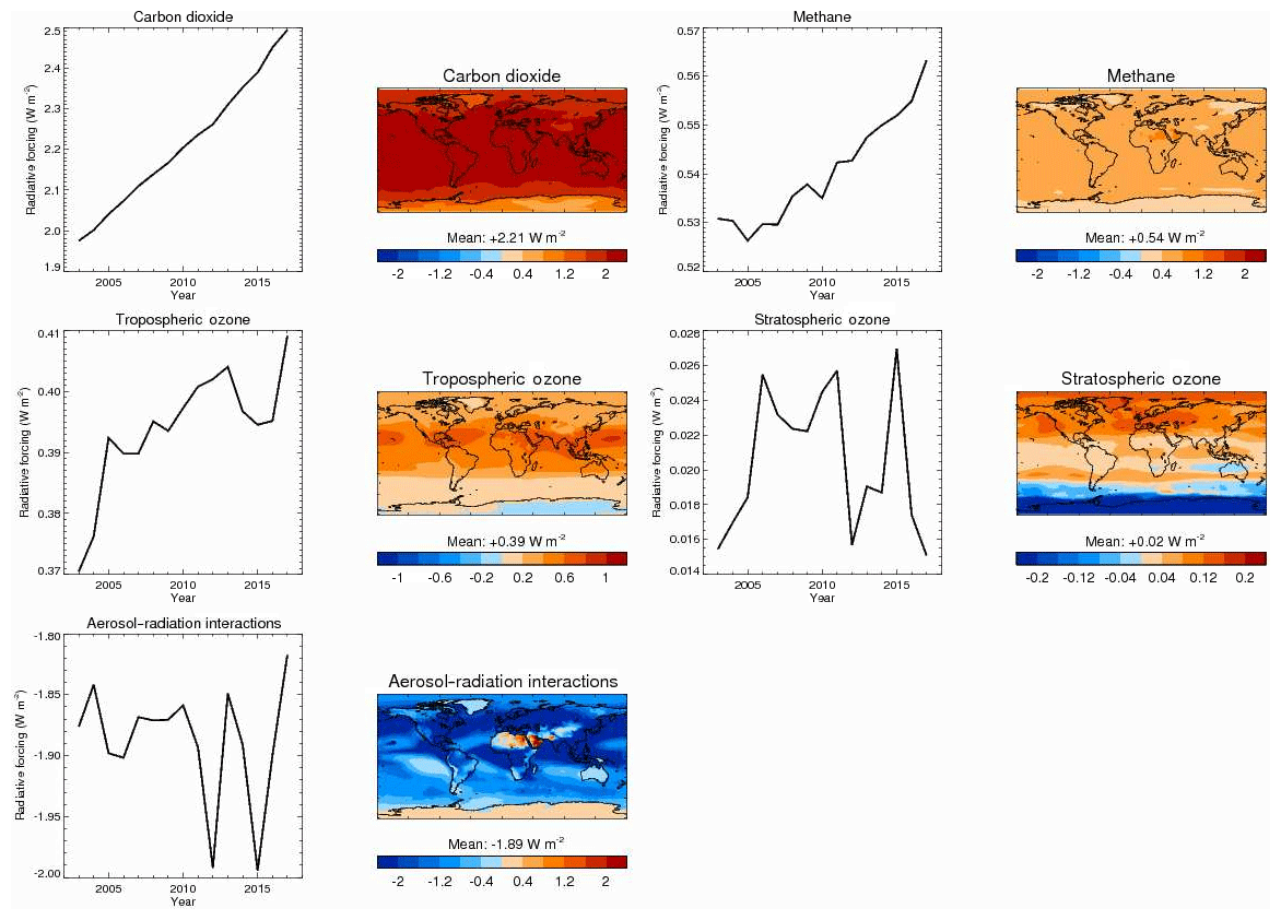
Figure 11As in Fig. 10 but for cloud-free conditions. Note that radiative forcing of aerosol–cloud interactions is undefined in the absence of clouds, so is not shown here.
Clouds exert a sizable modulation of RF. Figure 11 shows the RF time series and average distributions in cloud-free conditions. This is estimated by setting cloud amounts to zero in radiative-transfer calculations but keeping other variables, in particular water vapour, fixed. Results suggest that RF would generally be stronger, in terms of absolute magnitude, in the absence of clouds. Alternatively, the results can be formulated as clouds masking a fraction of cloud-free RF. Clouds mask 14 % of carbon dioxide and methane RF. That estimate is similar to the previous estimate of 13 % for carbon dioxide by Myhre et al. (1998) but smaller than the estimate of 29 % given for methane by Minschwaner et al. (1998). Clouds mask 17 % of tropospheric ozone RF and switch the sign of global-mean stratospheric ozone RF, which, however, remains weak. Clouds mask at least 70 % of RFari, this value being a lower bound because the CAMS estimate excludes a small contribution from above-cloud aerosol absorption. Interestingly, the net effect of clouds is to weaken total aerosol RF since RFaci is weaker than the fraction of RFari masked by clouds. Clouds have little effect on trends.
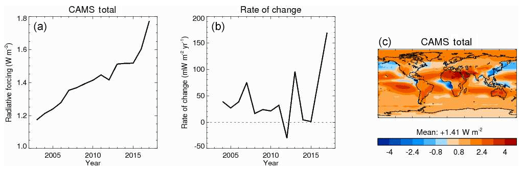
Figure 12(a) Time series of global annually averaged total stratospherically adjusted radiative forcing in the shortwave and longwave spectra (W m−2) for the period 2003–2017. Total radiative forcing is defined here as the sum of the radiative-forcing components shown in Fig. 10. (b) Rate of change in total radiative forcing, calculated as the change in total radiative forcing from a given year to the next (in mW m−2 yr−1). (c) Distribution of total stratospherically adjusted radiative forcing, averaged over the period 2003–2017 (in W m−2).
Figure 12 shows the time evolution, average distribution, and rate of change of total RF over the period 2003–2017. Here, the rate of change is calculated as the change in total RF from one year to the next. Total RF is obtained by adding the CAMS estimates of the RF of carbon dioxide, methane, ozone, and aerosols. Total RF is estimated at +1.17 W m−2 in 2003 and has increased to +1.77 W m−2 in 2017. The fact that total RF has become more positive over the period indicates driving of further increases in surface temperatures. Total RF is positive over most of the globe, with peaks in the Tropics, where carbon dioxide, methane, and tropospheric ozone RF peak. RF is also large at high latitudes of the Northern Hemisphere for two reasons. First, this is where both tropospheric and stratospheric ozone contribute large positive RF. Second, this is where RFaci is not estimated because the satellite retrievals on which the estimate relies are biased due to large solar zenith angles (see Sect. 2.3). There are a few regions where aerosol RF more than offsets the RF of the other forcing agents, leading to a negative total RF. This happens in the North Pacific and over China but also off the coast of biomass-burning regions in West Africa and the Maritime Continent, although neglecting above-cloud RFari may exaggerate the offset. Rates of change in total RF have varied over the period but generally remained between 20 and 70 mW m−2 yr−1. The years 2012, 2014, and 2015 have slower rates, less than 10 mW m−2 yr−1 because of a slowdown in methane RF increase and a large aerosol RF, respectively. The years 2013 and 2017 have rates above 90 mW m−2 yr−1 because of a weaker aerosol RF combined, for 2017, with a strong methane forcing. Note that Fig. 12 and its analysis does not account for the contribution of, and changes in, radiative-forcing agents that are not estimated in CAMS, notably nitrous oxide and halocarbons, surface albedo and land use changes, and solar and volcanic RF.
Table 8Comparison of best estimate and 5 %–95 % confidence ranges for stratospherically adjusted radiative forcing (in W m−2) as assessed by the Fifth Assessment Report (AR5) of the Intergovernmental Panel on Climate Change (IPCC; Sect. 8.3.2 and Table 8.6 of Myhre et al., 2013a) and obtained by this study, both for 2011 relative to 1750. AR5 estimates for aerosol–cloud interactions are for the effective radiative forcing.
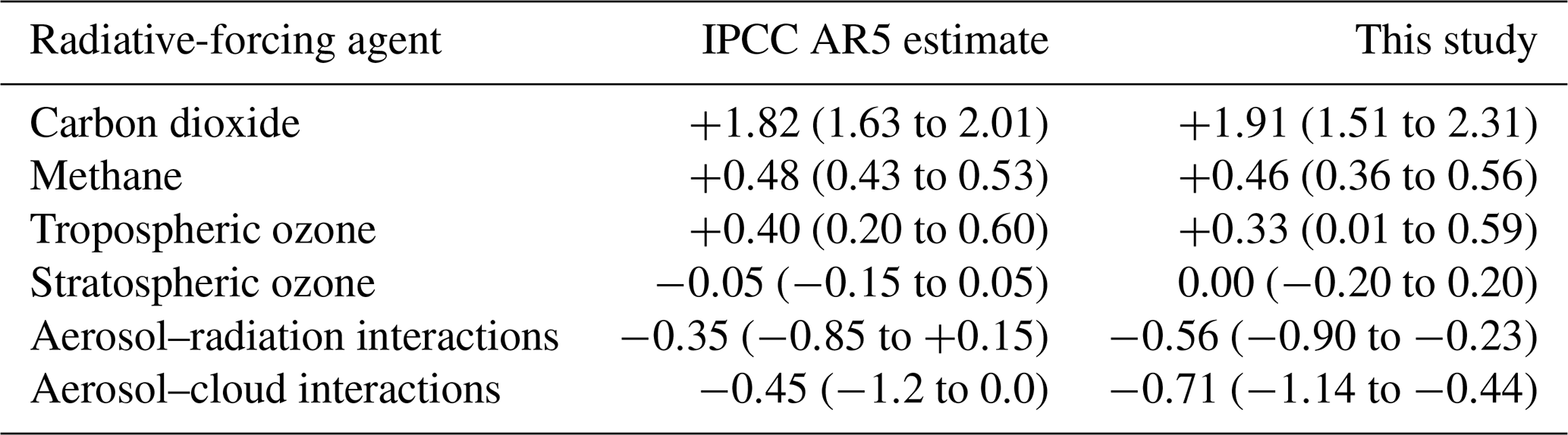
Our more consistent treatment of forcing agents led to CAMS Climate Forcing estimates and uncertainties within previously assessed ranges but with noticeable differences for aerosols. In CAMS, the 1σ uncertainty range for carbon dioxide and methane forcing is estimated at 13 %, slightly larger than the 10 % uncertainty generally assumed in IPCC Assessment Reports. The uncertainty ranges for ozone and aerosols are larger, at 50 % for tropospheric ozone, 100 % for stratospheric ozone, and 38 % for total aerosol radiative forcing. The IPCC AR5 provides estimates for the year 2011, so they are compared to the same year from the CAMS dataset (Table 8). CAMS best estimates are close to those made at the time of the AR5, with the exception of RFari and RFaci, which are 60 % stronger in CAMS than in AR5, although these are still within assessed uncertainty ranges. RFari and RFaci are also consistent with the recent assessment by Bellouin et al. (2020a). CAMS uncertainty ranges are wider (although not greatly so) than assessed in AR5 because we have assessed a much more comprehensive set of uncertainty sources than AR5.
5.2 Carbon dioxide and methane
The CAMS estimates of RF by carbon dioxide and methane are based on the three-dimensional distributions of CAMS greenhouse gas flux inversions. Most previous estimates are either based on radiative-transfer calculations that assume a uniform mixing ratio of these gases or use simplified expressions, especially those by Myhre et al. (1998), obtained by fitting the calculations of radiative-transfer models of varying spectral resolution. Figure 13 compares the CAMS estimates to calculations using the same methods and input datasets, except that carbon dioxide and methane are now prescribed uniformly as measured by the ESRL and AGAGE networks (see Sect. 2.1 and Fig. 2). The year 2017 is not included in that comparison because calculations with uniform concentrations have only been done for the period 2003–2016. Pre-industrial concentrations are set to 278 ppm for carbon dioxide and 722 ppb for methane, like in Sect. 3.1. Also included in the comparison are estimates from the simplified expressions in Table 3 of Myhre et al. (1998), calculated using annually averaged mass-weighted atmospheric concentrations from the CAMS greenhouse gas flux inversions. Calculations assume the same pre-industrial concentrations as above and in addition assume a pre-industrial concentration of 270 ppb for nitrous oxide (again from Table 8.2 of Myhre et al., 2013a), which is a required input for the methane forcing calculation.
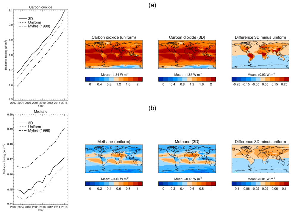
Figure 13Comparison of stratospherically adjusted radiative forcing (in W m−2) of carbon dioxide (a) and methane (b) based on either the three-dimensional distributions produced by CAMS Greenhouse Gas Flux or the surface measurements of the NOAA Earth System Research Laboratory for carbon dioxide and the Advanced Global Atmospheric Gases Experiment for methane. Corresponding concentration time series are shown in Fig. 2. Panels on the left show time series for 2003–2016, with radiative forcing from three-dimensional distributions shown as a solid line, from uniform concentrations as a dashed line, and from the simplified expressions of Myhre et al. (1998) as a dotted–dashed line. Maps show, from left to right, the distributions from three-dimensional distributions, from uniform concentrations, and their difference.
Three-dimensional distributions yield a slightly larger RF than uniform distributions, but the differences are only within 1 % to 2 %. Such small differences agree with past studies done on methane RF (Freckleton et al., 1998; Minschwaner et al., 1998), although they did not include shortwave effects and so obtained a different sign for the difference. Differences are likely due to saturation of RF as concentrations increase: RF has a logarithmic dependence on concentrations for carbon dioxide and a square-root dependence for methane, and concentrations are effectively lower in the three-dimensional case (Fig. 2). The increase in RF is contributed by land surfaces, where distributions depart most from uniformity because of local anthropogenic and natural sources. Three-dimensional distributions yield a stronger carbon dioxide RF but a weaker methane RF than simplified expressions, but again differences are small compared to overall uncertainties.
5.3 Ozone
Although we presented tropospheric and stratospheric ozone forcing separately in Sect. 5.1, based on our tropopause definition, we recognise that there is some artificiality in the separation. Although stratospheric ozone change is primarily driven by ozone-depleting substances (ODS), modelling studies indicate a compensatory increase in stratospheric ozone due to emissions of gases conventionally regarded as tropospheric ozone precursors (carbon monoxide, methane and nitrous oxides). Similarly, ODS affect tropospheric ozone, mostly via changes in stratosphere-troposphere exchange. Søvde et al. (2011, 2012), for 1850–2000, and Shindell et al. (2013b), for 1850–2005, estimate that the precursors offset about 35 %–40 % of the negative stratospheric RF due to ODS, while about 15 % of the positive tropospheric ozone forcing due to precursors is offset by ODS. For the total ozone RF, ODS offset about half of the positive forcing due to the precursors.
In that context, it is interesting to look at total ozone RF, the sum of tropospheric and stratospheric ozone RFs. Figure 14 shows time series and distributions of total ozone RF for the period 2003–2017. After an increase from 2003 to 2005, dominated by an increase in tropospheric ozone concentrations, total ozone RF has been stable around 0.32 W m−2. In terms of distribution, ozone RF is positive over most of the globe, with a maximum in the tropical Northern Hemisphere. The high latitudes of the Southern Hemisphere are, however, associated with a negative ozone RF, due to stratospheric ozone depletion.
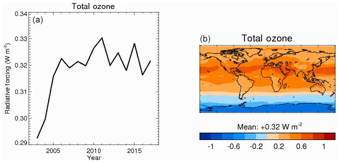
Figure 14Annual and global-mean time series and average distribution for the CAMS reanalysis period (2003–2017) of the stratospherically adjusted radiative forcing of ozone (relative to 1750 and in W m−2), calculated as the sum of tropospheric and stratospheric ozone radiative forcing. Radiative forcing is given for shortwave plus longwave.
5.4 Aerosols
Because aerosols have short residence times in the troposphere, on the order of 1 week, distributions of trends in their concentrations and radiative forcing are driven by changes in aerosol primary and precursor emissions, which are themselves driven by air quality policy and economic decisions, at least over industrial regions. Figure 15 shows deseasonalised trends in anthropogenic AOD as estimated by the aerosol origin identification algorithm described in Sect. 3.3 applied to the CAMS reanalysis for the period 2003–2017. Although globally averaged anthropogenic AOD shows essentially no trend over the period, this hides very large regional trends. According to the CAMS reanalysis, total AOD has decreased over the eastern United States, Europe, South America, and China and increased over India and Siberia (Rémy et al., 2019). As shown in Fig. 15, the aerosol origin identification algorithm attributes those trends to anthropogenic aerosols, except for the Siberian trends, despite the Siberian trends being most probably caused by an increase in wildfires in the region. Decreasing aerosol amounts in China after about 2010 are confirmed by analyses of satellite aerosol retrievals and ground-based sun photometers (Filonchyk et al., 2019) and air quality monitoring (Zheng et al., 2018). Both studies detect the start of the decrease in 2013 and attribute it to the implementation of China's Clean Air Action. Over South America, Aragão et al. (2018) report a decrease in deforestation rates over 2003–2015, which is expected to be associated with a decreasing trend in biomass-burning aerosol emissions. Over India, analyses of ground-based remote sensing measurements confirm the increasing trend and attribute it to an increase in anthropogenic emissions (Babu et al., 2013; Satheesh et al., 2017). Figure 15 also shows wide oceanic regions, especially in the southern Pacific and Southern Ocean, associated with small but statistically significant positive trends. Those trends may not be real, as they are smaller than the 0.001 yr−1 drift in AOD that may affect the MODIS Collection 6.1 retrievals (Levy et al., 2018) that are assimilated in the CAMS reanalysis. Those trends could also reveal shortcomings of the aerosol identification algorithm or be real trends caused by biomass-burning aerosols transported from the Maritime Continent, South America, and Africa. The confidence in those trends and in the associated RFari and RFaci in these regions is therefore low.
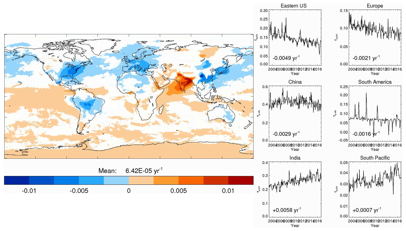
Figure 15Linear trends (yr−1) in anthropogenic aerosol optical depth at 0.55 µm over the period 2003–2017 according to the CAMS Climate Forcing aerosol origin identification algorithm. Regions where trends are statistically insignificant are masked in white. Right-hand-side plots show time series of anthropogenic aerosol optical depth (τanth; solid lines) and their linear fits (dashed lines) in selected regions.
Copernicus Climate Forcings data are available for download at https://doi.org/10.24380/ads.1hj3y896 (Bellouin et al., 2020b). Copernicus data are free and open access.
Monthly distributions of CAMS RF at the surface, tropopause, and TOA and in clear- and all-sky conditions are available for download at https://doi.org/10.24380/ads.1hj3y896 (Bellouin et al., 2020b). Monthly distributions of anthropogenic AOD and aerosol radiative effects for mineral dust, marine, anthropogenic, and land-based fine-mode aerosols are also available. The availability of RF estimates resolved in space and time is rare, so the CAMS RF dataset has the potential to serve several categories of climate researchers. Some of the needs can be readily satisfied with the current products, while others will require further co-construction with the users. We have identified a number of areas where the CAMS RF are already in use or could be used.
-
Monitoring climate forcings is a key element in monitoring the climate system. The CAMS RF estimates are now routinely included in the AMS State of the Climate reports published each year in the BAMS (see https://www.ametsoc.org/index.cfm/ams/publications/bulletin-of-the-american-meteorological-society-bams/state-of-the-climate/, last access: 14 July 2020). Other regular climate assessments (IPCC, WMO) could also benefit from the CAMS products.
-
Many scientists, governments, intergovernmental bodies, and non-governmental organisations are monitoring the evolution of climate change, the progress of international climate mitigation towards carbon neutrality, and the implications for the remaining carbon budget. Present-day radiative forcing for non-CO2 greenhouse gases and aerosols and its year-to-year evolution are key knowledge elements for estimating the remaining carbon budget, the year when carbon neutrality needs to be achieved, and asymptotic permissible emissions if and when the climate is stabilised.
-
Detection and attribution of climate change relies on the observed climate record (typically surface temperature), the modelled patterns of climate change response to the most relevant climate forcings (well-mixed greenhouse gases, ozone, aerosols, land-use change, etc.), a priori estimates of the temporal evolution of these forcings, and appropriate statistical methods. The regional dimension to such attribution studies is becoming increasingly important (see, e.g. Stott et al., 2010). Knowledge of the climate sensitivity is hindered by the lack of knowledge on RFs (in particular aerosol RF) and vice versa (Forest, 2018). Such attribution studies are now being extended to extreme events (Otto et al., 2016) with similar requirements on climate forcings when it comes to model the climate response. An improved knowledge of anthropogenic RFs is therefore highly relevant for detection and attribution of climate change.
-
Decadal prediction has emerged as a new concept in climate science and lies between seasonal to interannual forecasting and longer-term (typically centennial) climate projections. The focus is on regional climate conditions over the next 10–30 years because of the importance of this timescale for adaptation to climate change (e.g. planning of infrastructure, management of water resources). Both internally generated variability and external radiative forcings contribute to decadal timescale climate change, and skill has been shown to arise from both factors. Knowledge of radiative forcings, especially at the regional scale and for the recent past, is therefore key to identifying future near-term trends in forcings that may provide predictability at the interannual to decadal timescales (Bellucci et al., 2015). In this context, up-to-date aerosol radiative forcing could prove a very useful resource for initialising the models used for decadal prediction.
-
Integrated assessment models (IAM) seek to integrate knowledge from both climate and socio-economic modelling in order to design and analyse future socio-economic pathways that comply with specific objectives (in particular climate objectives). IAM usually rely on simplified climate models and need to calibrate their estimates of radiative forcings. Earth System Models of Intermediate Complexity (EMICs) and compact models such as FaIR (Smith et al., 2018b) or OSCAR (Gasser et al., 2017) also have the same requirement and could possibly be further calibrated and/or evaluated using recent trends in radiative forcings.
Note that many of the uses listed above require RF estimates for a more comprehensive list of climate forcing agents than is currently available from CAMS. Adding missing gases, such as nitrous oxide and halocarbons, and mechanisms, such as stratospheric water vapour, are possible future extensions to the service.
Table 9Global, multi-annual mean top-of-atmosphere instantaneous radiative forcing (IRF), rapid adjustments (RA), and scaling factor for the rapid adjustments from PDRMIP models (Myhre et al., 2018).
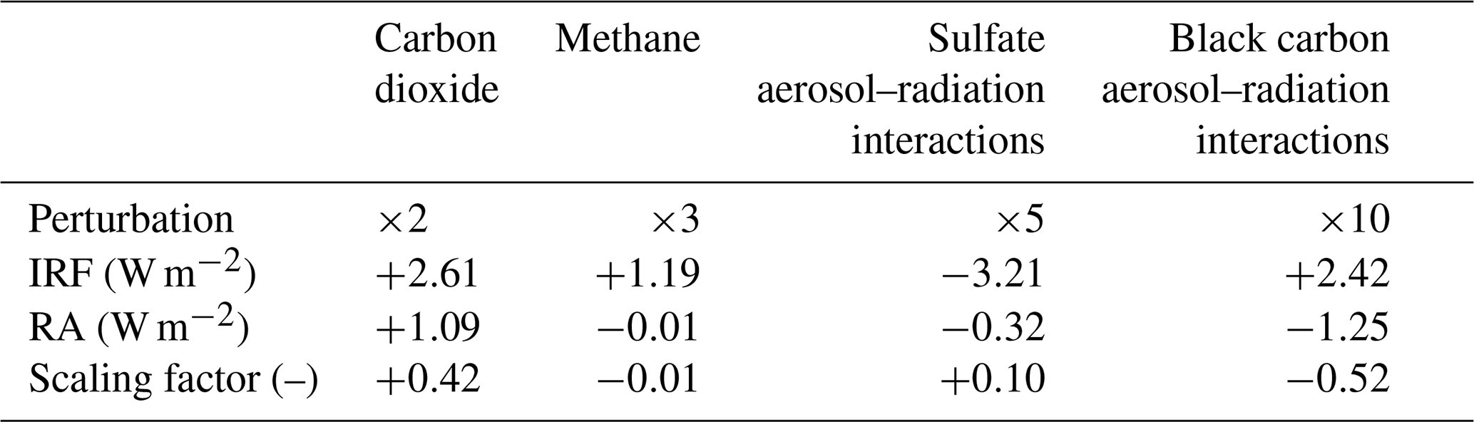
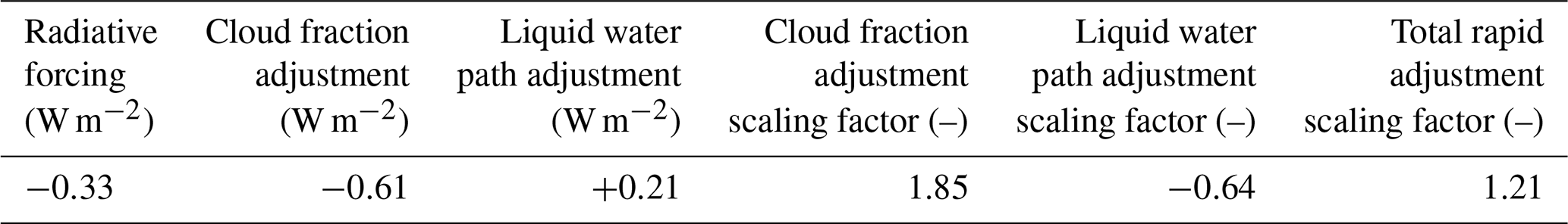
Table 10Radiative forcing of aerosol–cloud interactions and cloud fraction and liquid water path adjustments, estimated using satellite retrieval statistics by Gryspeerdt et al. (2019). The scaling factors for each rapid adjustment and the total rapid adjustment are also provided. Values are for all present-day anthropogenic aerosols.
The CAMS project estimates IRF and RF, but doe not yet estimate ERF. ERF involves adjustments in atmospheric temperature, moisture, and cloudiness, which are not easy to quantify using offline radiative-transfer calculations. One possibility is to estimate rapid adjustments from scaling factors derived from simulations by the Precipitation Driver-Response Model Intercomparison Project (PDRMIP; Myhre et al., 2017). The scaling factors (SF) would be calculated as the ratio of rapid adjustments (RA) to IRF, where instantaneous means that stratospheric adjustments are not included:
ERF would then be calculated as follows:
Table 9 lists potential scaling factors, taken from Smith et al. (2018a) and Myhre et al. (2018). Rapid adjustments for carbon dioxide are mostly exerted by adjustments to stratospheric temperature. Tropospheric rapid adjustments are virtually zero, as also found by Vial et al. (2013) using models participating in the Fifth Coupled Model Intercomparison Project (CMIP5). So the CAMS RF estimates would not need to be corrected further. Methane does not exert substantial rapid adjustments on a global average. However, its scaling factor is more uncertain (as discussed in Smith et al., 2018a) because the subset of PDRMIP models that include methane shortwave absorption have a different scaling factor to those that only simulate methane absorption in the longwave. The adjustments exerted by aerosol species are essentially located in the troposphere and are large compared to the IRF. For absorbing black carbon aerosols, rapid adjustments offset half of the positive IRF. It is not possible to use global climate models to estimate rapid adjustments from aerosol–cloud interaction because they are unable to properly represent the relevant physical processes (Toll et al., 2017). Global statistics of satellite aerosol and cloud retrievals would be used instead. For aerosol–cloud interactions, two aspects of rapid adjustments need to be considered: the response of cloud liquid water path and of cloud fraction. For these, the statistical approach of Gryspeerdt et al. (2016) and the scaling factors derived by Gryspeerdt et al. (2019) could be used, as summarised in Table 10. There is, however, currently no literature on rapid adjustments in the troposphere for ozone RF.
There are also plans to explore uncertainties further. The pre-industrial state is an important contributor to RF uncertainty, especially for aerosols (Carslaw et al., 2013), so using multiple realisations of it would improve the quantification of the associated uncertainty. A range of credible pre-industrial states could be achieved with IFS simulations using (1) CMIP6 emissions, where pre-industrial wildfires are scaled down from present-day according to population changes; (2) present-day Global Fire Assimilation System emissions, where biomass-burning could be assumed to have been unchanged over the industrial era; and (3) emissions from Hamilton et al. (2018), which correspond to a pre-industrial state where wildfires were more widespread than represented in CMIP6. Finally, the current assessment of uncertainty combines a PPE, where aerosol optical properties and atmospheric state variables were varied within their prescribed uncertainty ranges, and a structural uncertainty analysis from climatological averaging, selection of radiation code, tropopause definition, and grid spacing. Some uncertain sources will have been neglected by only perturbing 24 parameters, and a more robust quantification of the uncertainty could be achieved if more parameters were perturbed. In addition, future work will perform a variance-based sensitivity analysis on the perturbed parameter ensemble to determine which components of the PPE contribute most to the variance in IRF.
NB leads CAMS Climate Forcings and coordinated the writing of the manuscript. NB, WD, JQ, JM, CS, and NS contributed to sections of the manuscript. All authors commented on draft versions of the manuscript.
The authors declare that they have no conflict of interest.
The Copernicus Atmosphere Monitoring Service (CAMS) is operated by the European Centre for Medium-Range Weather Forecasts on behalf of the European Commission as part of the Copernicus Programme (http://copernicus.eu, last access: 14 July 2020). The authors thank Vincent-Henri Peuch, Richard Engelen, and Johannes Flemming for their leadership of CAMS.
This research has been supported by the European Centre for Medium Range Weather Forecasts (grant no. ECMWF/COPERNICUS/2016/CAMS_74_UoR).
This paper was edited by David Carlson and reviewed by two anonymous referees.
Aragão, L. E. O. C., Anderson, L. O., Fonseca, M. G., Rosan, T. M., Vedovato, L. B., Wagner, F. H., Silva, C. V. J., Silva Jr., C. H. L., Arai, E., Aguiar, A. P., Barlow, J., Berenguer, E., Deeter, M. N., Domingues, L. G., Gatti, L., Gloor, M., Malhi, Y., Marengo, J. A., Miller, J. B., Phillips, O. L., and Saatchi, S.: 21st Century drought-related fires counteract the decline of Amazon deforestation carbon emissions, Nat. Commun., 9, 536, https://doi.org/10.1038/s41467-017-02771-y, 2018.
Asmi, A., Wiedensohler, A., Laj, P., Fjaeraa, A.-M., Sellegri, K., Birmili, W., Weingartner, E., Baltensperger, U., Zdimal, V., Zikova, N., Putaud, J.-P., Marinoni, A., Tunved, P., Hansson, H.-C., Fiebig, M., Kivekäs, N., Lihavainen, H., Asmi, E., Ulevicius, V., Aalto, P. P., Swietlicki, E., Kristensson, A., Mihalopoulos, N., Kalivitis, N., Kalapov, I., Kiss, G., de Leeuw, G., Henzing, B., Harrison, R. M., Beddows, D., O'Dowd, C., Jennings, S. G., Flentje, H., Weinhold, K., Meinhardt, F., Ries, L., and Kulmala, M.: Number size distributions and seasonality of submicron particles in Europe 2008–2009, Atmos. Chem. Phys., 11, 5505–5538, https://doi.org/10.5194/acp-11-5505-2011, 2011.
Babu, S. S., Manoj, M. R., Moorthy, K. K., Gogoi, M. M., Nair, V. S., Kompalli, S. K., Satheesh, S. K., Niranjan, K., Ramagopal, K., Bhuyan, P. K., and Singh, D.: Trends in aerosol optical depth over Indian region: Potential causes and impact indicators, J. Geophys. Res.-Atmos., 118, 11794–11806, https://doi.org/10.1002/2013JD020507, 2013.
Bauer, P., Thorpe, A., and Brunet, G.: The quiet revolution of numerical weather prediction, Nature, 525, 47–55, https://doi.org/10.1038/nature14956, 2015.
Bellouin, N., Jones, A., Haywood, J., and Christopher, S. A.: Updated estimate of aerosol direct radiative forcing from satellite observations and comparison against the Hadley Centre climate model, J. Geophys. Res., 113, D10205, https://doi.org/10.1029/2007JD009385, 2008.
Bellouin, N., Quaas, J., Morcrette, J.-J., and Boucher, O.: Estimates of aerosol radiative forcing from the MACC re-analysis, Atmos. Chem. Phys., 13, 2045–2062, https://doi.org/10.5194/acp-13-2045-2013, 2013.
Bellouin, N., Quaas, J., Gryspeerdt, E., Kinne, S., Stier, P., Watson-Parris, D., Boucher, O., Carslaw, K. S., Christensen, M., Daniau, A.-L., Dufresne, J.-L., Feingold, G., Fiedler, S., Forster, P., Gettelman, A., Haywood, J.M., Lohmann, U., Malavelle, F., Mauritsen, T., McCoy, D.T., Myhre, G., Muelmenstaedt, J., Neubauer, D., Possner, A., Rugenstein, M., Sato, Y., Schulz, M., Schwartz, S. E., Sourdeval, O., Storelvmo, T., Toll, V., Winker, D., and Stevens, B.: Bounding global aerosol radiative forcing of climate change, Rev. Geophys., 58, e2019RG000660. https://doi.org/10.1029/2019RG000660, 2020a.
Bellouin, N., Davies, W., Shine, K. P., Quaas, J., Mülmenstädt, J., Forster, P. M., Smith, C., Lee, L., Regayre, L., Brasseur, G., Sudarchikova, N., Bouarar, I., Boucher, O., and Myhre, G.: Supplemental Data of Radiative forcing of climate change from the Copernicus reanalysis of atmospheric composition, ECMWF Data catalogue, https://doi.org/10.24380/ads.1hj3y896, 2020b.
Bellucci, A., Haarsma, R., Bellouin, N., Booth, B., Cagnazzo, C., Hurk, B., Keenlyside, N., Koenigk, T., Massonnet, F., Materia, S., and Weiss, M.: Advancements in decadal climate predictability: The role of non-oceanic drivers, Rev. Geophys., 53, 165–202, https://doi.org/10.1002/2014RG000473, 2015.
Benedetti, A., Morcrette, J.‐J., Boucher, O., Dethof, A., Engelen, R. J., Fisher, M., Flentje, H., Huneeus, N., Jones, L., Kaiser, J. W., Kinne, S., Mangold, A., Razinger, M., Simmons, A. J., and Suttie, M.: Aerosol analysis and forecast in the European Centre for Medium-Range Weather Forecasts Integrated Forecast System: 2. Data assimilation, J. Geophys. Res., 114, D13205, https://doi.org/10.1029/2008JD011115, 2009.
Bergamaschi, P., Houweling, S., Segers, A., Krol, M., Frankenberg, C., Scheepmaker, R. A., Dlugokencky, E., Wofsy, S. C., Kort, E. A., Sweeney, C., Schuck, T., Brenninkmeijer, C., Chen, H., Beck, V., and Gerbig, C.: Atmospheric CH4 in the first decade of the 21st century: Inverse modeling analysis using SCIAMACHY satellite retrievals and NOAA surface measurements, J. Geophys. Res.-Atmos., 118, 7350–7369, https://doi.org/10.1002/jgrd.50480, 2013.
Bond, T. C., Doherty, S. J., Fahey, D. W., Forster, P. M., Berntsen, T., DeAngelo, B. J., Flanner, M. G., Ghan, S., Kärcher, B., Koch, D., Kinne, S., Kondo, Y., Quinn, P. K., Sarofim, M. C., Schultz, M. G., Schulz, M., Venkataraman, C., Zhang, H., Zhang, S., Bellouin, N., Guttikunda, S. K., Hopke, P. K., Jacobson, M. Z., Kaiser, J. W., Klimont, Z., Lohmann, U., Schwarz, J. P., Shindell, D., Storelvmo, T., Warren, S. G., and Zender, C. S.: Bounding the role of black carbon in the climate system: A scientific assessment, J. Geophys. Res., 118, 5380–5552, https://doi.org/10.1002/jgrd.50171, 2013.
Boucher, O., Randall, D., Artaxo, P., Bretherton, C., Feingold, G., Forster, P., Kerminen, V.-M., Kondo, Y., Liao, H., Lohmann, U., Rasch, P., Satheesh, S. K., Sherwood, S., Stevens, B., and Zhang, X. Y.: Clouds and aerosols, in: Climate change 2013: The physical science basis. Contribution of Working Group I to the Fifth Assessment Report of the Intergovernmental Panel on Climate Change, edited by: Stocker, T. F., Qin, D., Plattner, G.-K., Tignor, M., Allen, S. K., Boschung, J., Nauels, A., Xia, Y., Bex, V., and Midgley, P. M., Cambridge University Press, Cambridge, UK and New York, NY, USA, 571–658, https://doi.org/10.1017/CBO9781107415324.016, 2013.
Carslaw, K. S., Lee, L. A., Reddington, C. L., Pringle, K. J., Rap, A., Forster, P. M., Mann, G. W., Spracklen, D. V., Woodhouse, M. T., Regayre, L. A., and Pierce, J. R.: Large contribution of natural aerosols to uncertainty in indirect forcing, Nature, 503, 7474, https://doi.org/10.1038/nature12674, 2013.
Checa-Garcia, R., Hegglin, M. I., Kinnison, D., Plummer, D. A., and Shine, K. P.: Historical tropospheric and stratospheric ozone radiative forcing using the CMIP6 database, Geophys. Res. Lett., 45, 3264–3273, https://doi.org/10.1002/2017GL076770, 2018.
Chevallier, F., Fisher, M., Peylin, P., Serrar, S., Bousquet, P., Bréon, F.-M., Chédin, A., and Ciais, P.: Inferring CO2 sources and sinks from satellite observations: Method and application to TOVS data, J. Geophys. Res., 110, D24309, https://doi.org/10.1029/2005JD006390, 2005.
Collins, W. D., Ramaswamy, V., Schwarzkopf, M. D., Sun, Y., Portmann, R. W., Fu, Q., Casanova, S. E. B., Dufresne, J.‐L., Fillmore, D. W., Forster, P. M. D., Galin, V. Y., Gohar, L. K., Ingram, W. J., Kratz, D. P., Lefebvre, M.‐P., Li, J., Marquet, P., Oinas, V., Tsushima, Y., Uchiyama, T., and Zhong, W. Y.: Radiative forcing by well-mixed greenhouse gases: Estimates from climate models in the Intergovernmental Panel on Climate Change (IPCC) Fourth Assessment Report (AR4), J. Geophys. Res., 111, D14317, https://doi.org/10.1029/2005JD006713, 2006.
Colman, R., Fraser, J., and Rotstayn, L.: Climate feedbacks in a general circulation model incorporating prognostic clouds, Clim. Dynam., 18, 103–122, https://doi.org/10.1007/s003820100162, 2001.
Conley, A. J., Lamarque, J.-F., Vitt, F., Collins, W. D., and Kiehl, J.: PORT, a CESM tool for the diagnosis of radiative forcing, Geosci. Model Dev., 6, 469–476, https://doi.org/10.5194/gmd-6-469-2013, 2013.
Dee, D. P., Uppala, S. M., Simmons, A. J., Berrisford, P., Poli, P., Kobayashi, S., Andrae, U., Balmaseda, M. A., Balsamo, G., Bauer, P., Bechtold, P., Beljaars, A. C. M., van de Berg, L., Bidlot, J., Bormann, N., Delsol, C., Dragani, R., Fuentes, M., Geer, A. J., Haimberger, L., Healy, S. B., Hersbach, H., Hólm, E. V., Isaksen, L., Kållberg, P., Köhler, M., Matricardi, M., McNally, A. P., Monge‐Sanz, B. M., Morcrette, J.‐J., Park, B.‐K., Peubey, C., de Rosnay, P., Tavolato, C., Thépaut, J.‐N., and Vitart, F. : The ERA-Interim reanalysis: configuration and performance of the data assimilation system, Q. J. Roy. Meteor. Soc., 137, 553–597, https://doi.org/10.1002/qj.828, 2011.
Dlugokencky, E. J., Hall, B. D., Montzka, S. A., Dutton, G., Mühle, J., and Elkins, J. W.: Long-lived greenhouse gases, in: State of the Climate in 2018, B. Am. Meteorol. Soc., 100, S48–S50, https://doi.org/10.1175/2019BAMSStateoftheClimate.1, 2019.
Dubovik, O., Holben, B., Eck, T. F., Smirnov, A., Kaufman, Y. J., King, M. D., Tanré, D., and Slutsker, I.: Variability of Absorption and Optical Properties of Key Aerosol Types Observed in Worldwide Locations. J. Atmos. Sci., 59, 590–608, https://doi.org/10.1175/1520-0469(2002)059<0590:VOAAOP>2.0.CO;2, 2002.
Etminan, M., Myhre, G., Highwood, E. J., and Shine, K. P.: Radiative forcing of carbon dioxide, methane, and nitrous oxide: A significant revision of the methane radiative forcing, Geophys. Res. Lett., 43, 12614–12623, https://doi.org/10.1002/2016GL071930, 2016.
Feng, Y., Ramanathan, V., and Kotamarthi, V. R.: Brown carbon: a significant atmospheric absorber of solar radiation?, Atmos. Chem. Phys., 13, 8607–8621, https://doi.org/10.5194/acp-13-8607-2013, 2013.
Filonchyk, M., Yan, H., Zhang, Z., Yang, S., Li, W., and Li, Y.: Combined use of satellite and surface observations to study aerosol optical depth in different regions of China, Sci, Rep., 9, 6174, https://doi.org/10.1038/s41598-019-42466-6, 2019.
Forest, C. E.: Inferred net aerosol forcing based on historical climate changes: a review, Curr. Clim. Change Rep., 4, 11–22, https://doi.org/10.1007/s40641-018-0085-2, 2018.
Forster, P., Ramaswamy, V., Artaxo, P., Berntsen, T., Betts, R., Fahey, D., Haywood, J., Lean, J., Lowe, D. C., Myhre, G., Nganga, J., Prinn, R., Raga, G., Schulz, M., and Van Dorland, R.: Changes in Atmospheric Constituentsand in Radiative Forcing, in: Climate change 2007: The physical science basis. Contribution of Working Group I to the Fourth Assessment Report of the Intergovernmental Panel on Climate Change, edited by: Solomon, S., Qin, D., Manning, M., Chen, Z., Marquis, M., Averyt, K. B., Tignor, M., and Miller, H. L., Cambridge University Press, Cambridge, UK and New York, NY, USA, 130–234, 2007.
Forster, P. M. D. and Shine, K. P.: Radiative forcing and temperature trends from stratospheric ozone changes, J. Geophys. Res.-Atmos., 102, 10841–10855, 1997.
Freckleton, R. S., Highwood, E. J., Shine, K. P., Wild, O., Law, K. S., and Sanderson, M. G.: Greenhouse gas radiative forcing: Effects of averaging and inhomogeneities in trace gas distribution, Q. J. Roy. Meteor. Soc., 124, 2099–2127, https://doi.org/10.1002/qj.49712455014, 1998.
Gasser, T., Ciais, P., Boucher, O., Quilcaille, Y., Tortora, M., Bopp, L., and Hauglustaine, D.: The compact Earth system model OSCAR v2.2: description and first results, Geosci. Model Dev., 10, 271–319, https://doi.org/10.5194/gmd-10-271-2017, 2017.
Gasteiger, J., Emde, C., Mayer, B., Buras, R., Buehler, S. A., and Lemke, O.: Representative wavelengths absorption parameterization applied to satellite channels and spectral bands, J. Quant. Spectrosc. Ra., 148, 99–115, https://doi.org/10.1016/j.jqsrt.2014.06.024, 2014.
Grosvenor, D. P., Sourdeval, O., Zuidema, P., Ackerman, A., Alexandrov, M. D., Bennartz, R., Boers, R., Cairns, B., Chiu, C., Christensen, M., Deneke, H., Diamond, M., Feingold, G., Fridlind, A., Hünerbein, A., Knist, C., Kollias, P., Marshak, A., McCoy, D., Merk, D., Painemal, D., Rausch, J., Rosenfeld, D., Russchenberg, H., Seifert, P., Sinclair, K., Stier, P., Van Diedenhoven, B., Wendisch, M., Werner, F., Wood, R., Zhang, Z., and Quaas, J.: Remote sensing of cloud droplet number concentration in warm clouds: A review of the current state of knowledge and perspectives, Rev. Geophys., 56, 409–453, https://doi.org/10.1029/2017RG000593, 2018.
Gryspeerdt, E., Quaas, J., and Bellouin, N.: Constraining the aerosol influence on cloud fraction, J. Geophys. Res., 121, 3566–3583, https://doi.org/10.1002/2015JD023744, 2016.
Gryspeerdt, E., Goren, T., Sourdeval, O., Quaas, J., Mülmenstädt, J., Dipu, S., Unglaub, C., Gettelman, A., and Christensen, M.: Constraining the aerosol influence on cloud liquid water path, Atmos. Chem. Phys., 19, 5331–5347, https://doi.org/10.5194/acp-19-5331-2019, 2019.
Hamilton, D. S., Hantson, S., Scott, C. E., Kaplan, J. O., Pringle, K. J., Nieradzik, L. P., Rap, A., Folberth, G. A., Spracklen, D. V., and Carslaw, K. S.: Reassessment of pre-industrial fire emissions strongly affects anthropogenic aerosol forcing, Nat. Commun., 9, 3182, https://doi.org/10.1038/s41467-018-05592-9, 2018.
Hansen, J., Sato, M., and Ruedy, R.: Radiative forcing and climate response, J. Geophys. Res., 102, 6831–6864, https://doi.org/10.1029/96JD03436, 1997.
Hartmann, D. L., Klein Tank, A. M. G., Rusticucci, M., Alexander, L. V., Brönnimann, S., Charabi, Y., Dentener, F. J., Dlugokencky, E. J., Easterling, D. R., Kaplan, A., Soden, B. J., Thorne, P. W., Wild, M., and Zhai, P. M.: Observations: Atmosphere and Surface, in: Climate Change 2013: The Physical Science Basis. Contribution of Working Group I to the Fifth Assessment Report of the Intergovernmental Panel on Climate Change, edited by: Stocker, T. F., Qin, D., Plattner, G.-K., Tignor, M., Allen, S. K., Boschung, J., Nauels, A., Xia, Y., Bex, V., and Midgley, P. M., Cambridge University Press, Cambridge, UK and New York, NY, USA, 2013.
Haywood, J. and Boucher, O.: Estimates of the direct and indirect radiative forcing due to tropospheric aerosols: A review, Rev. Geophys., 38, 513–543, https://doi.org/10.1029/1999RG000078, 2000.
Hegglin, M., Kinnison, D., Lamarque, J.-F., and Plummer, D.: CCMI ozone in support of CMIP6 – version 1.0, Earth System Grid Federation, https://doi.org/10.22033/ESGF/input4MIPs.1115, 2016.
Hogan, R. J. and Bozzo, A.: A flexible and efficient radiation scheme for the ECMWF model, J. Adv. Model. Earth Syst., 10, 1990–2008, https://doi.org/10.1029/2018MS001364, 2018.
Hollingsworth, A., Engelen, R. J., Textor, C., Benedetti, A., Boucher, O., Chevallier, F., Dethof, A., Elbern, H., Eskes, H., Flemming, J., Granier, C., Kaiser, J. W., Morcrette, J., Rayner, P., Peuch, V., Rouil, L., Schultz, M. G., and Simmons, A. J.: Toward A Monitoring And Forecasting System For Atmospheric Composition, B. Am. Meteorol. Soc., 89, 1147–1164, https://doi.org/10.1175/2008BAMS2355.1, 2008.
Inness, A., Blechschmidt, A.-M., Bouarar, I., Chabrillat, S., Crepulja, M., Engelen, R. J., Eskes, H., Flemming, J., Gaudel, A., Hendrick, F., Huijnen, V., Jones, L., Kapsomenakis, J., Katragkou, E., Keppens, A., Langerock, B., de Mazière, M., Melas, D., Parrington, M., Peuch, V. H., Razinger, M., Richter, A., Schultz, M. G., Suttie, M., Thouret, V., Vrekoussis, M., Wagner, A., and Zerefos, C.: Data assimilation of satellite-retrieved ozone, carbon monoxide and nitrogen dioxide with ECMWF's Composition-IFS, Atmos. Chem. Phys., 15, 5275–5303, https://doi.org/10.5194/acp-15-5275-2015, 2015.
Inness, A., Ades, M., Agustí-Panareda, A., Barré, J., Benedictow, A., Blechschmidt, A.-M., Dominguez, J. J., Engelen, R., Eskes, H., Flemming, J., Huijnen, V., Jones, L., Kipling, Z., Massart, S., Parrington, M., Peuch, V.-H., Razinger, M., Remy, S., Schulz, M., and Suttie, M.: The CAMS reanalysis of atmospheric composition, Atmos. Chem. Phys., 19, 3515–3556, https://doi.org/10.5194/acp-19-3515-2019, 2019.
Johnson, J. S., Regayre, L. A., Yoshioka, M., Pringle, K. J., Lee, L. A., Sexton, D. M. H., Rostron, J. W., Booth, B. B. B., and Carslaw, K. S.: The importance of comprehensive parameter sampling and multiple observations for robust constraint of aerosol radiative forcing, Atmos. Chem. Phys., 18, 13031–13053, https://doi.org/10.5194/acp-18-13031-2018, 2018.
Kacenelenbogen, M. S., Vaughan, M. A., Redemann, J., Young, S. A., Liu, Z., Hu, Y., Omar, A. H., LeBlanc, S., Shinozuka, Y., Livingston, J., Zhang, Q., and Powell, K. A.: Estimations of global shortwave direct aerosol radiative effects above opaque water clouds using a combination of A-Train satellite sensors, Atmos. Chem. Phys., 19, 4933–4962, https://doi.org/10.5194/acp-19-4933-2019, 2019.
Kato, S., Loeb, N. G., Rose, F. G., Doelling, D. R., Rutan, D. A., Caldwell, T. E., Yu, L., and Weller, R. A.: Surface Irradiances Consistent with CERES-Derived Top-of-Atmosphere Shortwave and Longwave Irradiances, J. Climate, 26, 2719–2740, https://doi.org/10.1175/JCLI-D-12-00436.1, 2013.
Kinne, S., Schulz, M., Textor, C., Guibert, S., Balkanski, Y., Bauer, S. E., Berntsen, T., Berglen, T. F., Boucher, O., Chin, M., Collins, W., Dentener, F., Diehl, T., Easter, R., Feichter, J., Fillmore, D., Ghan, S., Ginoux, P., Gong, S., Grini, A., Hendricks, J., Herzog, M., Horowitz, L., Isaksen, I., Iversen, T., Kirkevåg, A., Kloster, S., Koch, D., Kristjansson, J. E., Krol, M., Lauer, A., Lamarque, J. F., Lesins, G., Liu, X., Lohmann, U., Montanaro, V., Myhre, G., Penner, J., Pitari, G., Reddy, S., Seland, O., Stier, P., Takemura, T., and Tie, X.: An AeroCom initial assessment – optical properties in aerosol component modules of global models, Atmos. Chem. Phys., 6, 1815–1834, https://doi.org/10.5194/acp-6-1815-2006, 2006.
Kinne, S., O'Donnel, D., Stier, P., Kloster, S., Zhang, K., Schmidt, H., Rast, S., Giorgetta, M., Eck, T. F., and Stevens, B.: MAC-v1: A new global aerosol climatology for climate studies, J. Adv. Model. Earth Syst., 5, 704–740, https://doi.org/10.1002/jame.20035, 2013.
Lamarque, J.-F., Bond, T. C., Eyring, V., Granier, C., Heil, A., Klimont, Z., Lee, D., Liousse, C., Mieville, A., Owen, B., Schultz, M. G., Shindell, D., Smith, S. J., Stehfest, E., Van Aardenne, J., Cooper, O. R., Kainuma, M., Mahowald, N., McConnell, J. R., Naik, V., Riahi, K., and van Vuuren, D. P.: Historical (1850–2000) gridded anthropogenic and biomass burning emissions of reactive gases and aerosols: methodology and application, Atmos. Chem. Phys., 10, 7017–7039, https://doi.org/10.5194/acp-10-7017-2010, 2010.
Lee, L. A., Carslaw, K. S., Pringle, K. J., Mann, G. W., and Spracklen, D. V.: Emulation of a complex global aerosol model to quantify sensitivity to uncertain parameters, Atmos. Chem. Phys., 11, 12253–12273, https://doi.org/10.5194/acp-11-12253-2011, 2011.
Lee, L. A., Pringle, K. J., Reddington, C. L., Mann, G. W., Stier, P., Spracklen, D. V., Pierce, J. R., and Carslaw, K. S.: The magnitude and causes of uncertainty in global model simulations of cloud condensation nuclei, Atmos. Chem. Phys., 13, 8879–8914, https://doi.org/10.5194/acp-13-8879-2013, 2013.
Levy, R. C., Mattoo, S., Sawyer, V., Shi, Y., Colarco, P. R., Lyapustin, A. I., Wang, Y., and Remer, L. A.: Exploring systematic offsets between aerosol products from the two MODIS sensors, Atmos. Meas. Tech., 11, 4073–4092, https://doi.org/10.5194/amt-11-4073-2018, 2018.
Lindsay, K., Bonan, G. B., Doney, S. C., Hoffman, F. M., Lawrence, D. M., Long, M. C., Mahowald, N. M., Keith Moore, J., Randerson, J. T., and Thornton, P. E.: Preindustrial-Control and Twentieth-Century Carbon Cycle Experiments with the Earth System Model CESM1(BGC), J. Climate, 27, 8981–9005, 2014.
Loeb, N. G., Doelling, D. R., Wang, H., Su, W., Nguyen, C., Corbett, J. G., Liang, L., Mitrescu, C., Rose, F. G., and Kato, S.: Clouds and the Earth's Radiant Energy System (CERES) Energy Balanced and Filled (EBAF) Top-of-Atmosphere (TOA) Edition-4.0 Data Product, J. Climate,, 31, 895–918, https://doi.org/10.1175/JCLI-D-17-0208.1, 2018.
Maclaurin, G., Sengupta, M., Xie, Y., and Gilroy, N.: Development of a MODIS-Derived Surface Albedo Data Set: An Improved Model Input for Processing the NSRDB. National Renewable Energy Laboratory Technical Report NREL/TP-6A20-67306, Golden, CO, USA, 23 pp., 2016.
Manners, J., Edwards, J. M., Hill, P., and Thelen, J. C.: SOCRATES Technical Guide: Suite Of Community RAdiative Transfer Codes Based on Edwards and Slingo, Technical Report, Met Office, Exeter, UK, 2017.
Mayer, B. and Kylling, A.: Technical note: The libRadtran software package for radiative transfer calculations – description and examples of use, Atmos. Chem. Phys., 5, 1855–1877, https://doi.org/10.5194/acp-5-1855-2005, 2005.
Meinshausen, M., Smith, S. J., Calvin, K., Daniel, J. S., Kainuma, M. L. T., Lamarque, J.-F., Matsumoto, K., Montzka, S. A., Raper, S. C. B., Riahi, K., Thomson, A., Velders, G. J. M., and van Vuuren, D. P. P.: The RCP greenhouse gas concentrations and their extensions from 1765 to 2300, Climatic Change, 109, 213, https://doi.org/10.1007/s10584-011-0156-z, 2011.
Minschwaner, K., Carver, R. W., Briegleb, B. P., and Roche, A. E.: Infrared radiative forcing and atmospheric lifetimes of trace species based on observations from UARS, J. Geophys. Res., 103, 23243–23253, https://doi.org/10.1029/98JD02116, 1998.
Mlawer, E. J., Taubman, S. J., Brown, P. D., Iacono, M. J., and Clough, S. A.: Radiative transfer for inhomogeneous atmospheres: RRTM, a validated correlated-k model for the longwave, J. Geophys. Res., 102, 16663–16682, https://doi.org/10.1029/97JD00237, 1997.
Morcrette, J.-J., Boucher, O., Jones, L., Salmond, D., Bechtold, P., Beljaars, A., Benedetti, A., Bonet, A., Kaiser, J. W., Razinger, M., Schulz, M., Serrar, S., Simmons, A. J., Sofiev, M., Suttie, M., Tompkins, A. M., and Untch, A.: Aerosol analysis and forecast in the ECMWF integrated forecast system: forward modeling, J. Geophys. Res., 114, D06206, https://doi.org/10.1029/2008JD011235, 2009.
Mülmenstädt, J., Gryspeerdt, E., Salzmann, M., Ma, P.-L., Dipu, S., and Quaas, J.: Separating radiative forcing by aerosol–cloud interactions and rapid cloud adjustments in the ECHAM–HAMMOZ aerosol–climate model using the method of partial radiative perturbations, Atmos. Chem. Phys., 19, 15415–15429, https://doi.org/10.5194/acp-19-15415-2019, 2019.
Myhre G., Highwood, E. J., Shine, K. P., and Stordal, F.: New estimates of radiative forcing due to well mixed greenhouse gases, Geophys. Res. Lett., 25, 2715–271, https://doi.org/10.1029/98GL01908, 1998.
Myhre, G., Shindell, D., Bréon, F.-M., Collins, W., Fuglestvedt, J., Huang, J., Koch, D., Lamarque, J.-F., Lee, D., Mendoza, B., Nakajima, T., Robock, A., Stephens, G., Takemura, T., and Zhang, H.: Anthropogenic and natural radiative forcing, in: Climate change 2013: The physical science basis. Contribution of Working Group I to the Fifth Assessment Report of the Intergovernmental Panel on Climate Change, edited by: Stocker, T. F., Qin, D., Plattner, G.-K., Tignor, M., Allen, S. K., Boschung, J., Nauels, A., Xia, Y., Bex, V., and Midgley, P. M., Cambridge University Press, Cambridge, UK and New York, NY, USA, 659–740, https://doi.org/10.1017/CBO9781107415324.018, 2013a.
Myhre, G., Samset, B. H., Schulz, M., Balkanski, Y., Bauer, S., Berntsen, T. K., Bian, H., Bellouin, N., Chin, M., Diehl, T., Easter, R. C., Feichter, J., Ghan, S. J., Hauglustaine, D., Iversen, T., Kinne, S., Kirkevåg, A., Lamarque, J.-F., Lin, G., Liu, X., Lund, M. T., Luo, G., Ma, X., van Noije, T., Penner, J. E., Rasch, P. J., Ruiz, A., Seland, Ø., Skeie, R. B., Stier, P., Takemura, T., Tsigaridis, K., Wang, P., Wang, Z., Xu, L., Yu, H., Yu, F., Yoon, J.-H., Zhang, K., Zhang, H., and Zhou, C.: Radiative forcing of the direct aerosol effect from AeroCom Phase II simulations, Atmos. Chem. Phys., 13, 1853–1877, https://doi.org/10.5194/acp-13-1853-2013, 2013b.
Myhre, G., Forster, P. M., Samset, B. H., Hodnebrog, Ø., Sillmann, J., Aalbergsjø, S. G., Andrews, T., Boucher, O., Faluvegi, G., Fläschner, D., Iversen, T., Kasoar, M., Kharin, V., Kirkevåg, A., Lamarque, J.-F., Olivié, D., Richardson, T. B., Shindell, D., Shine, K. P., Stjern, C. W., Takemura, T., Voulgarakis, A., and Zwiers, F.: PDRMIP: A Precipitation Driver and Response Model Intercomparison Project–Protocol and Preliminary Results, B. Am. Meteorol. Soc., 98, 1185–1198, https://doi.org/10.1175/BAMS-D-16-0019.1, 2017.
Myhre, G., Kramer, R. J., Smith, C. J., Hodnebrog, Ø., Forster, P., Soden, B. J., Samset, B. H., Stjern, C. W., Andrews, T., Boucher, O., Faluvegi, G., Fläschner, D., Kasoar, M. , Kirkevåg, A., Lamarque, J.‐F., Olivié, D., Richardson, T., Shindell, D., Stier, P., Takemura, T., Voulgarakis, A., and Watson‐Parris, D.: Quantifying the importance of rapid adjustments for global precipitation changes, Geophys. Res. Lett., 45, 11399–11405, https://doi.org/10.1029/2018GL079474, 2018.
Myhre, G., Samset, B. H., Mohr, C. W., Alterskjær, K., Balkanski, Y., Bellouin, N., Chin, M., Haywood, J., Hodnebrog, Ø., Kinne, S., Lin, G., Lund, M. T., Penner, J. E., Schulz, M., Schutgens, N., Skeie, R. B., Stier, P., Takemura, T., and Zhang, K.: Cloudy sky contributions to the direct aerosol effect, Atmos. Chem. Phys. Discuss., https://doi.org/10.5194/acp-2019-1051, in review, 2019.
Oikawa, E., Nakajima, T., and Winker, D.: An evaluation of the shortwave direct aerosol radiative forcing using CALIOP and MODIS observations, J. Geophys. Res.-Atmos., 123, 1211–1233, https://doi.org/10.1002/2017JD027247, 2018.
Otto, F. E. L., van Oldenborgh, G. L., Eden, J., Stott, P. A., Karoly, D. J., and Allen, M. R.: The attribution question, Nat. Clim. Chang., 6, 813–816, https://doi.org/10.1038/nclimate3089, 2016.
Pincus, R., Barker, H. W., and Morcrette, J.-J.: A fast, flexible, approximate technique for computing radiative transfer in inhomogeneous cloud fields, J. Geophys. Res., 108, 4376, https://doi.org/10.1029/2002JD003322, 2003.
Pincus, R., Mlawer, E. J., Oreopoulos, L., Ackerman, A. S., Baek, S., Brath, M., Buehler, S. A., Cady‐Pereira, K. E., Cole, J. N. S., Dufresne, J. L., Kelley, M., Li, J., Manners, J., Paynter, D. J., Roehrig, R., Sekiguchi, M., and Schwarzkopf, D. M.: Radiative flux and forcing parameterization error in aerosol-free clear skies, Geophys. Res. Lett., 42, 5485–5492, https://doi.org/10.1002/2015GL064291, 2015.
Pincus, R., Forster, P. M., and Stevens, B.: The Radiative Forcing Model Intercomparison Project (RFMIP): experimental protocol for CMIP6, Geosci. Model Dev., 9, 3447–3460, https://doi.org/10.5194/gmd-9-3447-2016, 2016.
Ramanathan, V.: Greenhouse Effect Due to Chlorofluorocarbons: Climatic Implications, Science, 190, 50–52, https://doi.org/10.1126/science.190.4209.50, 1975.
Ramaswamy, V., Boucher, O., Haigh, J., Hauglustaine, D., Haywood, J., Myhre, G., Nakajima, T., Shi, G. Y., and Solomon, S.: Radiative forcing of climate change, in: Climate change 2001: Working Group I: The Scientific Basis, edited by: Houghton, J. T., Ding, Y., Griggs, D. J., Noguer, M., van der Linden, P. J., Dai, X., Maskell, K., and Johnson, C. A., 351–416, Cambridge University Press, Cambridge, UK and New York, NY, USA, 2001.
Ramaswamy, V., Collins, W., Haywood, J., Lean, J., Mahowald, N., Myhre, G., Naik, V., Shine, K., Soden, B., Stenchikov, G., and Storelvmo, T.: Radiative Forcing of Climate: The Historical Evolution of the Radiative Forcing Concept, the Forcing Agents and their Quantification, and Applications, Meteor. Mon., 59, 14.1–14.101, https://doi.org/10.1175/AMSMONOGRAPHS-D-19-0001.1, 2019.
Randles, C. A., Kinne, S., Myhre, G., Schulz, M., Stier, P., Fischer, J., Doppler, L., Highwood, E., Ryder, C., Harris, B., Huttunen, J., Ma, Y., Pinker, R. T., Mayer, B., Neubauer, D., Hitzenberger, R., Oreopoulos, L., Lee, D., Pitari, G., Di Genova, G., Quaas, J., Rose, F. G., Kato, S., Rumbold, S. T., Vardavas, I., Hatzianastassiou, N., Matsoukas, C., Yu, H., Zhang, F., Zhang, H., and Lu, P.: Intercomparison of shortwave radiative transfer schemes in global aerosol modeling: results from the AeroCom Radiative Transfer Experiment, Atmos. Chem. Phys., 13, 2347–2379, https://doi.org/10.5194/acp-13-2347-2013, 2013.
Regayre, L. A., Pringle, K. J., B. Booth, B. B., Lee, L. A., Mann, G. W., Browse, J., Woodhouse, M. T., Rap, A., Reddington, C. L., and Carslaw, K. S.: Uncertainty in the magnitude of aerosol-cloud radiative forcing over recent decades, Geophys. Res. Lett., 41, 9040–9049, https://doi.org/10.1002/2014GL062029, 2014.
Regayre, L. A., Johnson, J. S., Yoshioka, M., Pringle, K. J., Sexton, D. M. H., Booth, B. B. B., Lee, L. A., Bellouin, N., and Carslaw, K. S.: Aerosol and physical atmosphere model parameters are both important sources of uncertainty in aerosol ERF, Atmos. Chem. Phys., 18, 9975–10006, https://doi.org/10.5194/acp-18-9975-2018, 2018.
Rémy, S., Bellouin, N., Kipling, Z., Ades, M., Benedetti, A., and Boucher, O.: Aerosols, in: “State of the Climate in 2018”, B. Am. Meteorol. Soc., 100, S52–S54, https://doi.org/10.1175/2019BAMSStateoftheClimate.1, 2019.
Satheesh, S. K., Suresh Babu, S., Padmakumari, B., Pandithurai, G., and Soni, V. K.: Variability of Atmospheric Aerosols Over India. Observed Climate Variability and Change over the Indian Region, edited by: Rajeevan, M. N. and Nayak, S., Springer Singapore, 221–248, https://doi.org/10.1007/978-981-10-2531-0_13, 2017.
Schaaf, C. B., Gao, F., Strahler, A. H., Lucht, W., Li, X., Tsang, T., Strugnell, N. C., Zhang, X., Jin, Y., Muller, J.-P., Lewis, P., Barnsley, M., Hobson, P., Disney, M., Roberts, G., Dunderdale, M., Doll, C., d'Entremont, R. P., Hu, B., Liang, S., Privette, J. L., and Roy, D.: First operational BRDF, albedo nadir reflectance products from MODIS, Remote Sens. Environ., 83, 135–148, https://doi.org/10.1016/S0034-4257(02)00091-3, 2002.
Schimel, D., Alves, D., Entling, I., Heimann, M., Joos, F., Raynaud, D., Wigley, T., Prather, M., Derwent, R., Ehhalt, D., Fraser, P., Sanhueza, E., Zhou, X., Jonas, P., Charlson, R., Rodhe, H., Sadasivan, S., Shine, K. P., Fouquart, Y., Ramaswamy, V., Solomon, S., Srinivasan, J., Albritton, D., Derwent, R., Isaksen, I., Lal, M., and Wuebbles, D.: Radiative forcing of climate change, in: Climate change 1995: The science of climate change. Contribution of Working Group I to the Second Assessment Report of the Intergovernmental Panel on Climate Change, edited by: Houghton, J. T., Meiro Filho, L. G., Callander, B. A., Harris, N., Kattenburg, A., and Maskell, K., Cambridge University Press, Cambridge, UK and New York, NY, USA, 69–131, 1996.
Sherwood, S. C., Bony, S., Boucher, O., Bretherton, C., Forster, P. M., Gregory, J. M., and Stevens, B.: Adjustments in the Forcing-Feedback Framework for Understanding Climate Change, B. Am. Meteorol. Soc., 96, 217–228, https://doi.org/10.1175/BAMS-D-13-00167.1, 2015.
Shindell, D. T., Lamarque, J.-F., Schulz, M., Flanner, M., Jiao, C., Chin, M., Young, P. J., Lee, Y. H., Rotstayn, L., Mahowald, N., Milly, G., Faluvegi, G., Balkanski, Y., Collins, W. J., Conley, A. J., Dalsoren, S., Easter, R., Ghan, S., Horowitz, L., Liu, X., Myhre, G., Nagashima, T., Naik, V., Rumbold, S. T., Skeie, R., Sudo, K., Szopa, S., Takemura, T., Voulgarakis, A., Yoon, J.-H., and Lo, F.: Radiative forcing in the ACCMIP historical and future climate simulations, Atmos. Chem. Phys., 13, 2939–2974, https://doi.org/10.5194/acp-13-2939-2013, 2013a.
Shindell, D., Faluvegi, G., Nazarenko, L., Bowman, K., Lamarque, J. F., Voulgarakis, A., Schmidt, G. A., Pechony, O., and Ruedy, R.: Attribution of historical ozone forcing to anthropogenic emissions, Nat. Clim. Chang., 3, 567–570, https://doi.org/10.1038/nclimate1835, 2013b.
Shine, K., Derwent, R. G., Wuebbles, D. J., Morcrette, J.-J., Apling, A. J., Blanchet, J. P., Charlson, R. J., Crommelynck, D., Grassl, H., Husson, N., Jenkins, G. J., Karol, I., King, M. D., Ramanathan, V., Rodhe, H., Shi, G.-Y., Thomas, G., Wang, W.-C., Wigley, T. M. L., Yamanouchi, T.: Radiative forcing of climate, in: Climate Change: The IPCC Scientific Assessment, edited by: Houghton, J. T., Jenkins, G. J., and Ephraums, J. J., 45–68, Cambridge University Press, Cambridge, UK and New York, NY, USA, 1990.
Smith, C. J., Kramer, R. J., Myhre, G., Forster, P. M., Soden, B. J., Andrews, T., Boucher, O., Faluvegi, G., Fläschner, D., Hodnebrog, Ø., Kasoar, M., Kharin, V., Kirkevåg, A., Lamarque, J.‐F., Mülmenstädt, J., Olivié, D., Richardson, T., Samset, B. H., Shindell, D., Stier, P., Takemura, T., Voulgarakis, A., and Watson‐Parris, D.: Understanding rapid adjustments to diverse forcing agents, Geophys. Res. Lett., 45, 12023–12031, https://doi.org/10.1029/2018GL079826, 2018a.
Smith, C. J., Forster, P. M., Allen, M., Leach, N., Millar, R. J., Passerello, G. A., and Regayre, L. A.: FAIR v1.3: a simple emissions-based impulse response and carbon cycle model, Geosci. Model Dev., 11, 2273–2297, https://doi.org/10.5194/gmd-11-2273-2018, 2018b.
Soden, B. J., Held, I. M., Colman, R., Shell, K. M., Kiehl, J. T., and Shields, C. A.: Quantifying Climate Feedbacks Using Radiative Kernels, J. Climate, 21, 3504–3520, https://doi.org/10.1175/2007JCLI2110.1, 2008.
Soden, B. J., Collins, W. D., and Feldman, D. R.: Reducing uncertainties in climate models, Science, 361, 326–327, https://doi.org/10.1126/science.aau1864, 2018.
Søvde, O. A., Hoyle, C. R., Myhre, G., and Isaksen, I. S. A.: The HNO3 forming branch of the HO2+NO reaction: pre-industrial-to-present trends in atmospheric species and radiative forcings, Atmos. Chem. Phys., 11, 8929–8943, https://doi.org/10.5194/acp-11-8929-2011, 2011.
Søvde, O. A., Hoyle, C. R., Myhre, G., and Isaksen, I. S. A.: Corrigendum to “The HNO3 forming branch of the HO2+NO reaction: pre-industrial-to-present trends in atmospheric species and radiative forcings” published in Atmos. Chem. Phys., 11, 8929–8943, 2011, Atmos. Chem. Phys., 12, 7725–7725, https://doi.org/10.5194/acp-12-7725-2012, 2012.
Stevenson, D. S., Young, P. J., Naik, V., Lamarque, J.-F., Shindell, D. T., Voulgarakis, A., Skeie, R. B., Dalsoren, S. B., Myhre, G., Berntsen, T. K., Folberth, G. A., Rumbold, S. T., Collins, W. J., MacKenzie, I. A., Doherty, R. M., Zeng, G., van Noije, T. P. C., Strunk, A., Bergmann, D., Cameron-Smith, P., Plummer, D. A., Strode, S. A., Horowitz, L., Lee, Y. H., Szopa, S., Sudo, K., Nagashima, T., Josse, B., Cionni, I., Righi, M., Eyring, V., Conley, A., Bowman, K. W., Wild, O., and Archibald, A.: Tropospheric ozone changes, radiative forcing and attribution to emissions in the Atmospheric Chemistry and Climate Model Intercomparison Project (ACCMIP), Atmos. Chem. Phys., 13, 3063–3085, https://doi.org/10.5194/acp-13-3063-2013, 2013.
Stott, P. A., Gillett, N. P., Hegerl, G. C., Karoly, D. J., Stone, D. A., Zhang, X., and Zwiers, F.: Detection and attribution of climate change: a regional perspective, WIREs Climate Change, 1, 192–211, https://doi.org/10.1002/wcc.34, 2010.
Taylor, J. P., Edwards, J. M., Glew, M. D., Hignett, P., and Slingo, A.: Studies with a flexible new radiation code. II: Comparisons with aircraft short-wave observations, Q. J. Roy. Meteor. Soc., 122, 839–862, 1996.
Toll, V., Christensen, M., Gassó, S., and Bellouin, N.: Volcano and ship tracks indicate excessive aerosol-induced cloud water increases in a climate model, Geophys. Res. Lett., 44, 12492–12500, https://doi.org/10.1002/2017GL075280, 2017.
Vial, J., Dufresne, J. L., and Bony, S.: On the interpretation of inter-model spread in CMIP5 climate sensitivity estimates, Clim. Dynam., 41, 3339, https://doi.org/10.1007/s00382-013-1725-9, 2013.
World Meteorological Organization (WMO): Executive Summary: Scientific Assessment of Ozone Depletion: 2018, Global Ozone Research and Monitoring Project–Report No. 58, Geneva, Switzerland, 67 pp., 2018.
Yeung, L. Y., Murray, L. T., Martinerie, P., Witrant, E., Hu, H., Banerjee, A., Orsi, A., and Chappellaz, J.: Isotopic constraint on the twentieth-century increase in tropospheric ozone, Nature, 570, 224–227, https://doi.org/10.1038/s41586-019-1277-1, 2019.
Young, P. J., Archibald, A. T., Bowman, K. W., Lamarque, J.-F., Naik, V., Stevenson, D. S., Tilmes, S., Voulgarakis, A., Wild, O., Bergmann, D., Cameron-Smith, P., Cionni, I., Collins, W. J., Dalsøren, S. B., Doherty, R. M., Eyring, V., Faluvegi, G., Horowitz, L. W., Josse, B., Lee, Y. H., MacKenzie, I. A., Nagashima, T., Plummer, D. A., Righi, M., Rumbold, S. T., Skeie, R. B., Shindell, D. T., Strode, S. A., Sudo, K., Szopa, S., and Zeng, G.: Pre-industrial to end 21st century projections of tropospheric ozone from the Atmospheric Chemistry and Climate Model Intercomparison Project (ACCMIP), Atmos. Chem. Phys., 13, 2063–2090, https://doi.org/10.5194/acp-13-2063-2013, 2013.
Yu, H., Chin, M., Remer, L. A., Kleidman, R. G., Bellouin, N., Bian, H., and Diehl, T.: Variability of marine aerosol fine‐mode fraction and estimates of anthropogenic aerosol component over cloud‐free oceans from the Moderate Resolution Imaging Spectroradiometer (MODIS), J. Geophys. Res., 114, D10206, https://doi.org/10.1029/2008JD010648, 2009.
Zhang, H., Zhu, S., Zhao, S., and Wei, X.: Establishment of High-resolution Aerosol Parameterization and Its Influence on Radiation Calculations, J. Quant. Spectrosc. Ra., 243, 106802, https://doi.org/10.1016/j.jqsrt.2019.106802, 2020.
Zheng, B., Tong, D., Li, M., Liu, F., Hong, C., Geng, G., Li, H., Li, X., Peng, L., Qi, J., Yan, L., Zhang, Y., Zhao, H., Zheng, Y., He, K., and Zhang, Q.: Trends in China's anthropogenic emissions since 2010 as the consequence of clean air actions, Atmos. Chem. Phys., 18, 14095–14111, https://doi.org/10.5194/acp-18-14095-2018, 2018.
Zuidema, P., Redemann, J., Haywood, J., Wood, R., Piketh, S., Hipondoka, M., and Formenti, P.: Smoke and clouds above the southeast Atlantic: Upcoming field campaigns probe absorbing aerosol's impact on climate, B. Am. Meteorol. Soc., 97, 1131–1135, https://doi.org/10.1175/BAMS-D-15-00082.1, 2016.