Annual dynamics of global land cover and its long-term changes from 1982 to 2015

Land cover is the physical material at the surface of the Earth. As the cause and result of global environmental change, land cover change (LCC) influences the global energy balance and biogeochemical cycles. Continuous and dynamic monitoring of global LC is urgently needed. Effective monitoring and comprehensive analysis of LCC at the global scale are rare. With the latest version of GLASS (Global Land Surface Satellite) CDRs (climate data records) from 1982 to 2015, we built the first record of 34-year-long annual dynamics of global land cover (GLASS-GLC) at 5 km resolution using the Google Earth Engine (GEE) platform. Compared to earlier global land cover (LC) products, GLASS-GLC is characterized by high consistency, more detail, and longer temporal coverage. The average overall accuracy for the 34 years each with seven classes, including cropland, forest, grassland, shrubland, tundra, barren land, and snow/ice, is 82.81 % based on 2431 test sample units. We implemented a systematic uncertainty analysis and carried out a comprehensive spatiotemporal pattern analysis. Significant changes at various scales were found, including barren land loss and cropland gain in the tropics, forest gain in the Northern Hemisphere, and grassland loss in Asia. A global quantitative analysis of human factors showed that the average human impact level in areas with significant LCC was about 25.49 %. The anthropogenic influence has a strong correlation with the noticeable vegetation gain, especially for forest. Based on GLASS-GLC, we can conduct long-term LCC analysis, improve our understanding of global environmental change, and mitigate its negative impact. GLASS-GLC will be further applied in Earth system modeling to facilitate research on global carbon and water cycling, vegetation dynamics, and climate change. The GLASS-GLC data set presented in this article is available at https://doi.org/10.1594/PANGAEA.913496 (Liu et al., 2020).

1 Introduction

Land cover (LC) is the physical material at the surface of the Earth. It is the result of both natural and human forces (Running, 2008; Sterling et al., 2013; Tucker et al., 1985; Gong et al., 2013; Yang et al., 2013). It is an important source of information to understand the complex interaction between human activities and global changes (Lambin et al., 2006). LC data are one of the most important variables to bring about the nine large social benefits in the field of Global Earth Observation Systems (Herold et al., 2008). Land cover change (LCC) is the cause and result of global environmental change (Turner et al., 2007), and it can change the energy balance and biogeochemical cycles (DeFries et al., 1999; Claussen et al., 2001), further affecting climate change and surface characteristics and the provision of ecosystem services (Pielke, 2005; Zhao et al., 2001; Gibbard et al., 2005; Reyers et al., 2009). Therefore, a long time series of LCC information is critical to the understanding of global environmental change (Matthews et al., 2004). LC and LCC information is also valuable to resource management, biodiversity conservation, food security, forest carbon, etc (Houghton et al., 2012; Achard et al., 2004; Andrew et al., 2015). Therefore, more frequent land cover information at the global scale is highly desirable.

However, LC is highly dynamic due to changes in natural phenology and human activities (Lambin et al., 2001). This characteristic poses a huge challenge to mapping, monitoring (Verburg et al., 2009; Lepers et al., 2005; Rindfuss et al., 2004), and quantitative analyses of global LCC (Ramankutty et al., 2006). The traditional method of LC mapping based on field studies can hardly be applied to large areas due to the required amount of labor (Gong, 2012). In addition, any mapping results obtained in this way would be difficult to update in a timely manner. Satellite observations are the most economically feasible means of large-scale LC monitoring (Fuller et al., 2003; Rogan and Chen, 2004). Due to the development of satellite sensors, the continuous accumulation of historical satellite data, and the advancement of relevant image processing algorithms, LC monitoring can be effectively carried out (Cihlar, 2000; Pal, 2005; Gallego, 2004; Chen et al., 2018). However, previous monitoring mainly focuses on the mapping of a particular area (Liu et al., 2002; Brink and Eva, 2009; Yuan et al., 2005; Margono et al., 2012; Feng et al., 2018) or in a single time period (Homer et al., 2004), and because of the differences in data sources and mapping methods, the consistency of mapping results from different sources and times is poor and lacks comparability, making it difficult to quantify the changes effectively (Friedl et al., 2010).

Automatic mapping methods depend highly on the sample data set due to its representativeness, quantity, and quality due to the considerable heterogeneity at the global level (Gong et al., 2013; Li et al., 2014). A combination of a comprehensive global sample data set, professional interpretation, and support from mapping teams are needed (Li et al., 2017). In general, sample LC data are mainly collected from field visits or manual interpretation (Li et al., 2016; Hansen et al., 2000). Generalization from higher-resolution LC map products can also be useful for coarser-resolution mapping purposes (X.-P. Song et al., 2018). The former could be more accurate and effective but requires a lot of manpower, resources, and effort (Li et al., 2016); the latter is a feasible option and is more efficient but largely dependant on the accuracy of the parent product.

A number of global LC products exist. Some examples include the Finer Resolution Observation and Monitoring of Global Land Cover product (FROM-GLC) in 2010, 2015, and 2017 (30 and 10 m) (Gong et al., 2013, 2019); European Space Agency Climate Change Initiative (ESA-CCI) land cover product from 1992 to 2015 (300 m) (ESA, 2018); MODIS Land Cover Type (MLCT) series products from 2001 to 2016 (500 m) (Friedl et al., 2010; Sulla-Menashe et al., 2019); International Geosphere–Biosphere Programme Data and Information System Cover map (IGBP-DISCover) (1 km) from circa 1992 (Loveland et al., 2000); University of Maryland (UMD) land cover map from circa 1992 (1 km) (Hansen et al., 2000); and Global Land Cover 2000 map (GLC2000) (1 km) (Bartholome and Belward, 2005). These mapping results tend to focus on a single or short period of time, and because of their different classification systems and resolutions, they are difficult to compare (Ban et al., 2015; Grekousis et al., 2015). However, high-resolution mapping results can be used as an effective reference for low-resolution mapping (X.-P. Song et al., 2018; DeFries et al., 1998). Therefore, when performing lower-resolution global mapping, it is possible to consider directly generating training samples from high-resolution global mapping results (Wang et al., 2016).

Long time series LC mapping requires a high consistency of data sources and also has certain requirements for multi-period samples (Huang et al., 2020). The commonly used satellite data that cover a long period of time (more than 30 years) include the Advanced Very High Resolution Radiometer (AVHRR) data and Landsat imagery (Giri et al., 2013; Franch et al., 2017; Wulder et al., 2018). Landsat data have a higher spatial resolution of 30 m with some restrictions, including a more serious cloud contamination problem owing to a low temporal frequency and a data inconsistency problem caused by multiple generations of sensors (Gómez et al., 2016; Wulder et al., 2008; Xie et al., 2018). AVHRR data have a low spatial resolution of 5 km, and the quality of the raw AVHRR data is poor. The requirements for preprocessing and consistency processing such as cloud removal and missing value filling are high. The GLASS (Global Land Surface Satellite) CDRs (climate data records) based on AVHRR data tend to have better data consistency due to systematic data production (Liang et al., 2013). Using such data for LC mapping can significantly improve the consistency and comparability of mapping results and thus can be effective in supporting change analysis. If the consistency of the original data source used is not good enough, it may be necessary to collect annual samples for classification to ensure the reliability of change analysis (Xu et al., 2018).

Recently, some attempts have been made to map global LC over a long time series, but these have focused on a single class, such as water bodies (Wood et al., 2011; Pekel et al., 2016; Ji et al., 2018), impervious surfaces (Schneider et al., 2010; Zhang and Seto, 2011; Gong et al., 2020), cropland (Pittman et al., 2010), or a few classes, such as Vegetation Continuous Fields (VCFs) (X.-P. Song et al., 2018), mainly depicting vegetation changes. General-purpose multi-class land cover mapping over a period of over 30 years does not exist.

Due to the lack of long time series general-purpose global LC maps, using the Google Earth Engine (GEE) platform (Gorelick et al., 2017), we produced the first CDR set of consistent and reliable LC products, GLASS-GLC, covering the period from 1982 to 2015. The data used was primarily the 0.05^∘ AVHRR-based GLASS CDRs. The classification system is adjusted from the FROM-GLC according to the data characteristics. Below, we describe the methods used and results obtained with some preliminary change analyses.

2 Data and methods

The framework for mapping GLASS-GLC is shown in Fig. 1. It includes annual input data collection and construction, training sample generation, classification, and temporal consistency adjustment, accuracy assessment, and product intercomparison. The entire framework is implemented in the GEE. The GEE is a cloud-based platform for planetary-scale geospatial analysis that brings Google's massive computational capabilities to bear on a variety of high-impact societal issues including deforestation, drought, disaster, disease, food security, water management, climate monitoring, and environmental protection (Gorelick et al., 2017). We uploaded GLASS data to GEE and performed subsequent analysis in GEE.

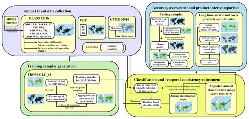
Figure 1 The framework for building GLASS-GLC (annual dynamics of global land cover) CDRs (climate data records).

2.1 Data sources

The annual input data collection from 1982 to 2015 involves a variety of data products, the most important of which is the latest version of Global Land Surface Satellite (GLASS) climate data records (CDRs) (Liang et al., 2013). CDRs require data with a long time series, high consistency and high continuity, which is not the same as the commonly used remote sensing products (Hollmann et al., 2013; Cao et al., 2008). Derived from AVHRR data, the GLASS CDRs include a wide range of surface parameters that are important to LC classification (GLASS, 2018). The products have a spatial resolution of 0.05^∘, a temporal frequency of 8 d, and a time span of 1982–2015. In our study, normalized difference vegetation index (NDVI), leaf area index (LAI) (Xiao et al., 2016), fraction of absorbed photosynthetically active radiation (FAPAR) (Xiao et al., 2015), evapotranspiration (ET) (Yao et al., 2014), gross primary production (GPP) (Yuan et al., 2010), broadband emissivity (BBE) (Cheng et al., 2016), white-sky albedo in the visible band (ABD-WSA-VIS) white-sky albedo in the near-infrared band (ABD-BSA-NIR), and white-sky albedo in the shortwave band (ABD-WSA-shortwave) (Qu et al., 2014) are the variables used for subsequent classification.

To provide a further reference, VCF5kyrv001 MEaSUREs Vegetation Continuous Fields (VCFs) Yearly Global 0.05 Deg products (Hansen, 2020) are used to aid classification. The VCF products describe the surface as a combination of vegetation proportions according to information from remotely sensed data. To match the resolution of the GLASS CDRs, the VCF products used here (X.-P. Song et al., 2018) also have a spatial resolution of 0.05^∘ and are obtained from the Land Processes Distributed Active Archive Center (LP DACC; available at https://lpdaac.usgs.gov/, last access: 1 November 2018). These products are mainly based on AVHRR, and the interannual consistency has been maintained. Based on the training samples from Landsat products from around 2000 (Hansen et al., 2013; Ying et al., 2017), with a supervised regression tree model, the VCF products from 1982 to 2016 (data missing in 1994 and 2000) were generated and were composed of the percentages of tree canopy (TC), short vegetation (SV), and bare ground (BG) in each pixel.

In addition, in order to enhance the discriminating capacity, we also used terrain data from Global Multi-resolution Terrain Elevation Data 2010 (GMTED2010). Based on the elevation data, the slope information can be further calculated to reflect the terrain and help distinguish different vegetation types growing on steep slopes to those on level ground. The data set comes from the GEE platform and contains Earth Elevation data collected from various sources (USGS, 2020). The primary source is the Shuttle Radar Topography Mission (SRTM) Digital Terrain Elevation Data (DTED) (void-filled) 1 arcsec data. Other sources are used for filling the gaps in areas outside the SRTM coverage. As the terrain is relatively stable over years, using the data as input for multiple years is plausible. The spatial resolution of the GMTED2010 data used is 7.5 arcsec and it has been up-sampled to 5 km in subsequent analyses.

2.2 Classification system

The classification system in FROM-GLC version 2 (FROM-GLC_v2) defines 11 main classes that can be easily mapped to the Food and Agricultural Organization of the United Nations (FAO) LC Classification System and the International Geosphere–Biosphere Programme (IGBP) classification system (Wang et al., 2015). This classification system evolved from the classification system of FROM-GLC version 1 (Gong et al., 2013) with the addition of leaf information.

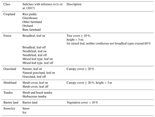
We adjusted some classes of the original classification system according to the spatial resolution and situation of the data used here. Our data are land surface products, where water surface has been masked out and the class of “water bodies” cannot be extracted from the GLASS data set. Wetland is a highly variable class and impervious surface with patches that are small in size. They are difficult to identify at the spatial resolution of 0.05^∘ (Wang et al., 2015). Thus, the water body, impervious surface, and wetland classes were not included in this work, and they shall be derived with more specialized methods. While water and impervious surface mapping have achieved satisfactory results (Ji et al., 2018; Gong et al., 2020), wetland mapping remains a great challenge (Gong et al., 2013). In addition, the “cloud” class was removed. The adjusted classification system consists of seven classes, including cropland, forest, grassland, shrubland, tundra, barren land, snow/ice, as shown in Table 1, where the snow/ice class here refers to permanent snow or ice cover.

Table 1 Classification system, with seven land cover classes.

2.3 Training samples

In order to obtain the training samples, we adopted the majority-class synthesis strategy. First, we projected the 30 m FROM-GLC_v2 results that were created using Landsat data acquired mainly from 2013 to 2015 (Li et al., 2017), into a 0.05^∘ coordinate system. By calculating the area ratio of each class in each 0.05^∘ pixel, the class with the greatest area ratio in each pixel was used as the new class label in the aggregated 0.05^∘ mapping results. Subsequently, sample points were randomly generated with greater than 0.1^∘ geographical distances from each other. The class label for each sample unit is obtained from the aggregated FROM-GLC_v2 0.05^∘ mapping result (adjusted to be consistent with the new classification system). Finally, 10 000 training sample units were obtained. The spatial distribution of training sample units is shown in Fig. 2a, and the percentage of training samples in each class is shown in the inner pie chart.

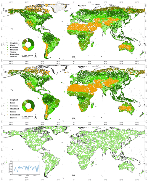
Figure 2 The geographical distribution training sample and test sample. (a) Training sample in 2015, where different colors represent the different classes. (b) Huge homogeneous test samples (H-homo sample) in 2015, where the different colors represent the source of the sample units, either FROM-GLC_v2 or FLUXNET. (c) Independent test sample in different years, where the temporal distribution is shown in the inner chart.

2.4 Input data collection

We constructed an input data set with a strong discrimination ability to detect LC from multiple aspects, such as terrain, phenology, spectrum, and spectral index. The annual percentiles (including 0, 10, 25, 50, 75, 90, 100) of all bands of the GLASS CDRs and the mean and standard deviation of the NDVI between two adjacent percentiles are calculated as an annual input data collection from GLASS CDRs. Among them, the percentile that represents specific phenological information can provide simplified time series information, reduce the noise of annual time series, and help improve the classification accuracy (Hansen et al., 2013). By extracting the statistical information between adjacent percentiles, the time series information can be further supplemented. Due to the systematic deviation of AVHRR products (Z. Song et al., 2018), and in order to ensure the interannual consistency of the GLASS data, we used the processing method developed for generating the VCF products, with the corresponding MODIS products for end-member correction, where desert and intact forest are regarded as the end-member of each pixel (X.-P. Song et al., 2018). After the correction, the interannual inconsistency of the input data collection from the GLASS CDRs is improved. Figure S1 in the Supplement shows the time series of the global median value of the GLASS ABD-WSA-VIS band, where the orange line represents the curve before the correction and the grey line is the result after the correction. It can be seen that, after the correction, the fluctuations of the input data become smaller and the individual abnormal values are also adjusted.

Taking into account the time span of the GLASS CDR-based input data collection, the VCF products from 1982 to 2015 are used, with the missing 1994 and 2000 data supplemented by calculating the average of the adjacent years. The VCF consists of percentages of tree cover (TC), short vegetation (SV), and bare ground (BG) for each year. Based on the GMTED2010 data set, the slope information is calculated and finally included to obtain an average slope value for each 0.05^∘ pixel. In addition, the central latitude and longitude information of each 0.05^∘ pixel is also recorded as part of the input data. Finally, an annual collection of 81 kinds of input for the period of 1982 to 2015 was constructed, including the annual GLASS CDR percentiles (7×9); the mean and standard deviation of the NDVI annual adjacent percentiles (6×2); and VCF percentages (3), slope information (1), latitude (1), and longitude (1) information (Table 2).

Table 2 The explanatory table of the constructed input data collection^*.

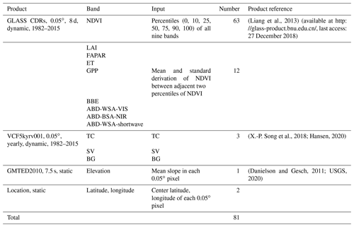
^* GLASS CDRs represent Global LAnd Surface Satellite (GLASS) climate data records (CDRs), VCF5kyrv001 stands for VCF5kyrv001 MEaSUREs Vegetation Continuous Fields (VCF) Yearly Global 0.05 Deg products, and GMTED2010 refers to Global Multi-resolution Terrain Elevation Data 2010. NDVI, LAI, FAPAR, ET, GPP, and BBE are abbreviations for normalized difference vegetation index, leaf area index, fraction of absorbed photosynthetically active radiation, evapotranspiration, gross primary production, and broadband emissivity, respectively. ABD-WSA-VIS, ABD-BSA-NIR, and ABD-WSA-shortwave represent white-sky albedo in visible band, near-infrared band, and shortwave band, respectively. TC, SV, and BG stand for tree canopy, short vegetation, and bare ground cover, respectively.

2.5 Classification method and temporal consistency check

We used a random forest classifier for global LC mapping following the good performance of the random forest classifier in the machine learning field (Rodriguez-Galiano et al., 2012; Pal, 2005). The number of trees was 200 with out-of-bag mode turned on. The number of variables per split was set to 0, as the square root of the number of variables. The minimum size of a terminal node, the fraction of input to bag per tree, and random seed were set to be 1, 0.5, and 0, respectively. The classifier was trained using the training sample with an annual data collection constructed as the input. The global LC maps from 1982 to 2015 were obtained using the trained classifier. The out-of-bag accuracy reached 87.12 %.

In order to further ensure the temporal consistency of the mapping results, we used the “LandTrendr” method (Kennedy et al., 2010; Cohen et al., 2018) and implemented a linear regression-based algorithm for the constructed annual input data collection to find the breakpoints in the time series (Li et al., 2018). The class labels in the time series between adjacent breakpoints will be updated to the mode values of the class label time series for the time period. Through this strategy, we can smooth the time series of the mapping results, avoid noise interference as much as possible, and finally get the adjusted GLASS-GLC.

2.6 Accuracy assessment

To verify the reliability of GLASS-GLC CDR products from multiple perspectives, we performed accuracy assessments and uncertainty analyses. The test sample was extracted from the 30 m resolution FROM-GLC_v2 (Li et al., 2017) to evaluate the 2015 LC mapping results. First, we dropped those sample units whose classes were not included in our classification system. The remaining test sample units were then overlapped with the abovementioned aggregated 0.05^∘ FROM-GLC_v2 mapping result, and only those whose class labels were consistent were kept. These were regarded as huge homogeneous sample units (H-homo sample) reserved as the final test sample. A total of 23 459 H-homo test sample units from FROM-GLC_v2 were obtained to test the 2015 global LC mapping result. In addition, another 525 test sample units from the FLUXNET site data (Gong, 2009) for 2015 were selected to supplement the test sample to test the 2015 result further. The distribution of the entire test sample in 2015 is shown in Fig. 2b, where the percentage of test sample for each class is shown in the inner pie chart.

In addition to obtaining the classification confusion matrix in 2015 based on the above test sample, in order to identify regions where classification is difficult, an uncertainty analysis was carried out. The incorrect test sample locations are marked as 1, while the correct test sample locations are marked as 0. The spatial distribution map of the uncertainty of the LC mapping result in 2015 is depicted based on a Kriging interpolation method (Oliver and Webster, 1990). The search radius parameter of Kriging interpolation is set to 12 nearby sample units, the other parameters as default. The value of the uncertainty ranges from 0 to 1. A value near 0 indicates a lower uncertainty, while a value near to 1 indicates a higher uncertainty and a higher possibility of misclassification.

Other than these, we collected an independent test sample and performed an accuracy assessment. Specifically, we collected 2431 randomly distributed 5 km sample points in different years around the world. According to the majority principle, we manually interpreted the land cover class of each sample as an independent test sample. To prove the impact of change detection, we further compared the accuracies with and without change detection. The geographical distribution of the independent test sample is shown in Fig. 2c, and the temporal distribution is shown in the inner chart.

2.7 Data intercomparison

To better reflect the product quality, We intercompared GLASS-GLC with other available global land cover products with a relatively long time series. Land cover products from MODIS and the ESA-CCI were used. The MLCT global land cover products come from Collection 6 (C6) MLCT products (Sulla-Menashe et al., 2019) and are supervised classification results from 2001 to 2016. Considering the comparability to our classification system, the FAO Land Cover Classification System land use (LCCS2) layer was used. The corresponding relationships of classes are listed as follows, and the class names we used are in parentheses: barren (barren land), permanent snow and ice (snow/ice), all kinds of forest (forest), forest/cropland mosaics and natural herbaceous/cropland mosaic (cropland), natural herbaceous and herbaceous cropland (grassland), and shrubland (shrubland). The ESA-CCI land cover products (Bontemps et al., 2013) are 300 m resolution yearly products ranging from 1992 to 2015. The products were developed using the GlobCover unsupervised classification chain and merging multiple available Earth observation products based on the GlobCover products of the ESA (Liu et al., 2018). Referring to the class relationships in Liu et al. (2018), we cross-walked classes including cropland, forest, grassland, shrubland, barren land, and snow/ice.

Apart from land cover products, we also compared GLASS-GLC with the Food and Agricultural Organization of the United Nations statistical data (FAOSTAT) on cropland and forest (forest land) classes, which are the main sources of country-level land cover data for many applications. The annual FAOSTAT data set for cropland that we used ranged from 1982 to 2015 and that which we used for forest ranged from 1990 to 2015.

We made an intercomparison between classes, including cropland, forest, grassland, shrubland, barren land, and snow/ice. The main intercomparison is the area corresponding to the top 50 countries in each class. Besides, to compare the accuracy of different products, test samples from FLUXNET site data in 2015 are given for independent accuracy assessment.

2.8 Statistical analysis of LCC

To extract the area of LCC, we estimated the trend of change through statistical analysis and avoided the influence of abnormal fluctuations from the obtained time series LC products. The annual area for each class on the scales of latitudinal zones, continents are summarized. A time series of the annual area for each class was generated. The boundary data of countries and continents were obtained from the Bureau of Surveying and Mapping of China. Eco-region data were obtained from the FAO global eco-region data set (Simons et al., 2001; FAO, 2018).

Although the interannual consistency has been ensured as much as possible in the above mapping framework, the effects of interannual changes due to climate conditions and phenological changes may still exist. To estimate the long-term trend of change, we fitted a linear trend (Theil–Sen estimator, Sen, 1968) in area for each class, where the slope of annual change and the 95 % confidence interval of the slope is given. In addition, a Mann–Kendall test (Mann, 1945) was used to test the trend of time series with a p value given. If p<0.05, it is considered that the trend of change is significant.

Further, we obtained the change mask where all pixels showed a significant change trend (Wang et al., 2016). First, we downscaled the grid from 0.05 to 0.25^∘, and the time series of the area ratio of all classes in each 0.25^∘ grid was summed. Using the Mann–Kendall test, those grids showing a significant change (p<0.05) were obtained. Then the slope of annual change based on area ratio for each grid with an increasing or decreasing trend was found using a Theil–Sen estimator. The change ratios were then summarized at regional scales to estimate the corresponding significant areas of change from 1982 to 2015.

In order to quantify the magnitude of global LCC between 1982 and 2015 and reveal the global temporal LCC pattern, we calculated the ratio of annual global LCC to the global total terrestrial LC area by different time periods. To ensure the quantified LCC was non-accidental, we limited the computation area within the change mask in which all grids show a statistically significant loss or gain trend. We then summarized the annual LCC by 5- and 10-year time intervals, respectively.

To further identify the direct causes of LCC, we assessed the LC conversion from 1982 to 2015. Based on the 0.05^∘ LC mapping results for 1982 and 2015, a map of LC conversion can be obtained. The computation was also limited to the change mask to ensure statistical significance. The conversion sources and destinations of LC classes were separately computed, to assess the direct causes of change in various LC classes.

Table 3 Classification accuracy of GLASS-GLC (annual dynamics of global land cover) in 2015 based on FROM-GLC_v2 (Finer Resolution Observation and Monitoring of Global Land Cover product version 2) test samples (overall accuracy =86.51 %; UA denotes user's accuracy, and PA denotes producer's accuracy). Bold numbers represent correctly classified samples.

Table 4 Classification accuracy of GLASS-GLC (annual dynamics of global land cover) in 2015 based on FLUXNET test samples (overall accuracy = 82.10 %; UA denotes user's accuracy, and PA denotes producer's accuracy). Bold numbers represent correctly classified ones.

2.9 Human impact process

To further explore the role of human impact in regions with significant LCC, the results are evaluated based on data from the human impact campaign (Fritz et al., 2017) (available at https://doi.org/10.1594/PANGAEA.869680, Fritz et al., 2016). The original study area was generated in the 2011 campaign to evaluate a map of land availability for biofuel production (Fritz et al., 2013) collected using a Geo-Wiki crowdsourcing platform. Pixels with a resolution of 1 km were randomly provided to volunteers. For each pixel, volunteers needed to point out the overall degree of human impact (HI, 0 %–100 %) that was visible from Google Earth's high-resolution satellite image, and they were required to provide confidence levels in four categories: unsure, less sure, quite sure, and sure. Here, HI refers to the degree to which the landscape modified by humans visible from satellite images (Fritz et al., 2017). A total of 151 942 point records are available. To get the global distribution map of HI, we performed Kriging interpolation on the point records that had previously excluded the category of unsure confidence level. The search radius parameter of the Kriging interpolation was set to 12 nearby points and the other parameters as default. As shown in Fig. S2, we can see that the interpolation results reflect the global distribution of the intensity of human activity.

Table 5 Classification accuracy of GLASS-GLC (annual dynamics of global land cover) without change detection under independent test samples (overall accuracy = 81.28 %; UA denotes user's accuracy, and PA denotes producer's accuracy). Bold numbers represent correctly classified ones.

Table 6 Classification accuracy of GLASS-GLC (annual dynamics of global land cover) with change detection under independent test samples (overall accuracy =82.81 %; UA denotes user's accuracy, and PA denotes producer's accuracy). Bold numbers represent correctly classified ones.

Figure 3 GLASS-GLC (annual dynamics of global land cover) CDRs (climate data records) results in 2015.

Figure 4 The geographical distribution of uncertainty for GLASS-GLC (annual dynamics of global land cover) CDRs (climate data records) in 2015, where regions in red represent higher uncertainty levels and those in green represent lower uncertainty levels.

3 Results

3.1 Reliability of the products

3.1.1 Accuracy assessment

First of all, to evaluate the magnitude of the errors introduced by our training samples, we randomly selected 500 samples from the training sample for manual interpretation and evaluation, and the assessment accuracy was 92.26 %. It shows that the training sample we generate from 30 m FROM-GLC_v2 is sufficient for our data production.

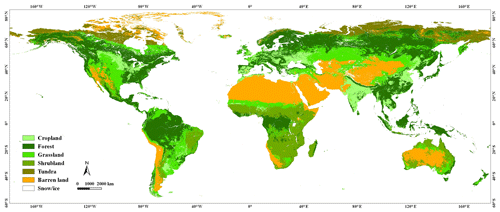
The global LC mapping result in 2015 is shown in Fig. 3. Its accuracy was tested with the H-homo sample in 2015 to obtain a confusion matrix (Table 3). The overall accuracy for the year 2015 reached 86.51 %. As for each class, the accuracies for forest, barren land, and tundra are relatively high, where the user's accuracies and producer's accuracies are over 90 %. The accuracy of cropland is also high, with the user's accuracy and producer's accuracy reaching 73.54 % and 78.62 %, respectively. The user's accuracy of shrubland reached 83.62 %, while that of grassland is 67.58 %. Grassland is mainly mixed with cropland and shrubland. Table 4 shows the testing results of the FLUXNET test samples in which the number of sample units for shrubland, tundra, barren land, and snow/ice are relatively small. The overall accuracy of all classes is 82.10 % with the FLUXNET sample. Among them, the user's accuracy and the producer's accuracy for forest reach 91.01 % and 88.04 %, respectively. The producer's accuracy for cropland is 69.23 %, while its user's accuracy is 73.26 %.

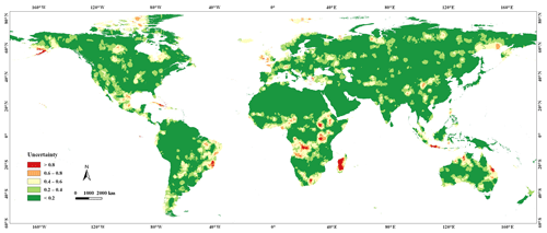
Putting the test results from FROM-GLC_v2 and FLUXNET together, a spatial distribution map of the uncertainty of the 2015 LC mapping result was generated. As can be seen from Fig. 4, most of the world is shown in green color, which means that the mapping result for most regions is most likely to be correct, and the result for 2015 is highly credible. There are still some regions showing a yellow or orange color, and a smaller number of regions showing red, representing those regions that may have been misclassified. Since there are no test samples in Greenland, the interpolation results are ignored. In general, the places with high uncertainty are Africa, eastern and southern South America  southern Alaska, northern and eastern Australia and southwestern Indonesia.

The assessment result with independent test samples is shown in Tables 5 and 6. It shows that the overall accuracy of the GLASS-GLC without change detection is 81.28 % and that with change detection is 82.81 %. This reflects the reliability of GLASS-GLC since the test samples are randomly distributed along the spatial and temporal dimensions, and also confirm the significance and effectiveness of the change detection method.

3.1.2 Data intercomparison

The assessment results of MLCT products and ESA-CCI land cover products based on test samples from FLUXNET site data are shown in Tables 7 and 8, respectively. The overall accuracies of ESA-CCI products and MLCT products are 73.90 % and 80.38 % in 2015, respectively. Compared to these, the overall accuracy of GLASS-GLC (82.10 %, Table 4) is better. Although the cross-walk of the different classification systems may be slightly different, It can still reflect the high accuracy of our GLASS-GLC products.

Table 7 Classification accuracy of the MLCT (MODIS Land Cover Type) product in 2015 based on FLUXNET test samples (overall accuracy = 82.10 %; UA denotes user's accuracy, and PA denotes producer's accuracy). Bold numbers represent correctly classified ones.

Table 8 Classification accuracy of the ESA-CCI (European Space Agency Climate Change Initiative) land cover product in 2015 based on FLUXNET test samples (overall accuracy = 82.10 %; UA denotes user's accuracy, and PA denotes producer's accuracy). Bold numbers represent correctly classified ones.

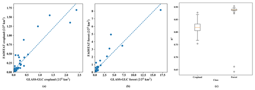
Figure 5 shows an intercomparison with MLCT products, Fig. 6 with ESA-CCI products, and Fig. 7 with FAOSTAT. The scatter plots and the linear fit lines reflected the results in 2015, and the box plots represent the distribution of R² of the annual linear fit lines for each class. It can be seen that various classes in several different products are relatively equivalent, although they are under different classification systems. In comparison with MLCT products, the results of 2001–2015 for cropland, forest, and snow/ice have high R². In comparison with ESA-CCI products, the mean R² of the linear fit lines of forest, grassland, and snow/ice from 1992 to 2015 reach 0.99, 0.82, and 0.98, respectively, while the R² for shrubland is low. The intercomparison of some other classes is poor, which may be caused by differences in the class definition in various classification systems. For instance, our classification system incorporates tundra, while the other two did not. Compared with FAOSTAT, the mean R² of the linear fit lines of cropland and forest is 0.82, and 0.87, respectively. In general, our GLASS-GLC products have a reasonable consistency with other products and statistics, and the difference is not significant. In addition to this, the duration of GLASS-GLC, 34 years, is much longer than MLCT and ESA-CCI land cover products (as shown in Fig. 8). The comparison with other data illustrates the reliability and accurateness of GLASS-GLC.

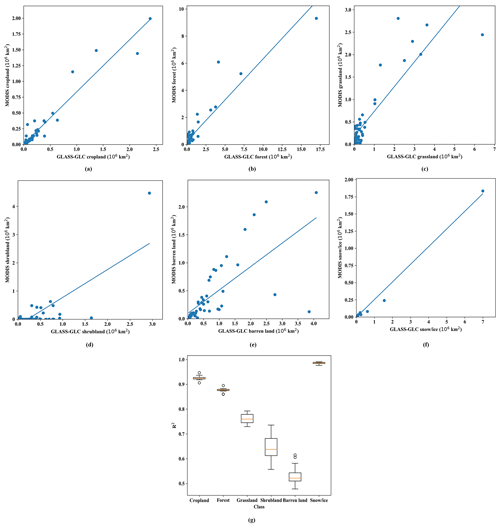
Figure 5 Intercomparison with the MLCT (MODIS Land Cover Type) product: (a) cropland circa 2015, (b) forest circa 2015, (c) grassland circa 2015, (d) shrubland circa 2015, (e) barren land circa 2015 and (f) snow/ice circa 2015; (g) mean R² of the annual linear fit lines for all years (2001–2015).

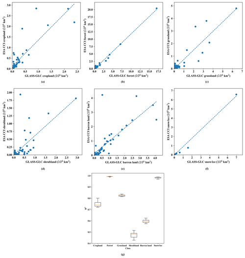
Figure 6 Intercomparison with the ESA-CCI (European Space Agency Climate Change Initiative) land cover product: (a) cropland circa 2015, (b) forest circa 2015, (c) grassland circa 2015, (d) shrubland circa 2015, (e) barren land circa 2015 and (f) snow/ice circa 2015; (g) mean R² of the annual linear fit lines for all years (1992–2015).

Figure 7 Intercomparison with the FAOSTAT data set: (a) cropland circa 2015, (b) forest circa 2015; (c) mean R² of the annual linear fit lines of cropland for years 1982–2015 and forest for years 1990–2015.

3.2 Spatiotemporal patterns in LCC

3.2.1 Global temporal patterns

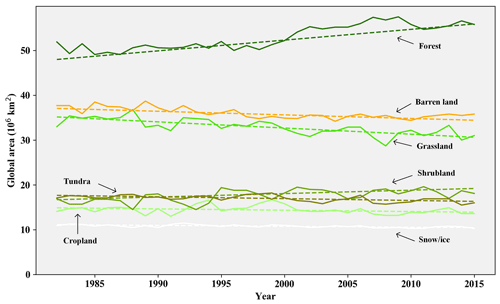
Figure 9 shows the temporal changes of the global area for various LC classes from 1982 to 2015, where dotted lines are the corresponding trend lines. Overall, the global area of forest increases significantly (p=0.0000) from 1982 to 2015. As for shrubland, although fluctuating, it shows a significant increasing trend (p=0.0017). The global area of grassland, tundra, barren land, and snow/ice significantly decreases with p=0.0000, p=0.0019, p=0.0000, and p=0.0003, respectively.

Figure 8 The duration of different land cover products, including the GLASS-GLC (annual dynamics of global land cover), MLCT (MODIS Land Cover Type), and ESA-CCI (European Space Agency Climate Change Initiative) land cover products.

Figure 9 Area curves of global annual land cover change from 1982 to 2015.

Figure 10 shows the annual ratio of the global LCC to the global total terrestrial area, shown and organized in different time periods, where Fig. 10a shows the results with a 5-year interval and Fig. 10b with a 10-year interval. Overall, the annual ratio ranges from 0.35 % to 0.70 %, with an average of 0.52 % between 1982 and 2015. The 5-year interval ratios show a relatively fluctuating trend. The average ratio reaches 0.63 % in 1991–1995, the highest among the seven intervals. The ratios had relatively large fluctuations in 2006–2010. All in all, the ratios before 1995 are generally higher, and have gradually decreased since then. With 10-year interval, ratios after 2000 are generally lower, with an average of only 0.40 % in 2011–2015.

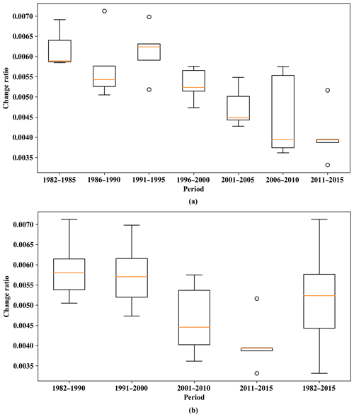
Figure 10 Comparison and distribution of ratios of annual global land cover change (LCC) to the global total terrestrial land cover (LC) area by different time periods and time intervals: (a) 5-year interval and (b) 10-year interval. The box extends from the first quartile (Q1) to third quartile (Q3) values of the data, with an orange line at the median. The upper whisker extends to the last datum less than Q3 $+\mathrm{1.5}\times$ IQR, and the lower whisker extends to the first datum greater than Q1 $-\mathrm{1.5}\times$ IQR. Flier points are those past the end of the whiskers.

3.2.2 Patterns along latitudinal gradients

The global distribution of 0.25^∘ grids with significant LCC from 1982 to 2015 is shown in Figs. 11 and S3 for the whole world, where the color depth represents the estimated change in area ratio per year. The distribution of significant LCC along latitudes is shown on the right, where the red curve represents a significant increase, green a significant decrease, and blue a net change.

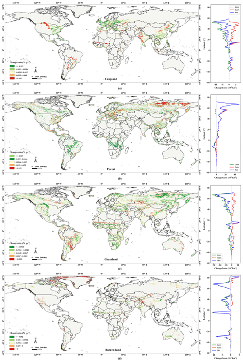
Figure 11 The geographical distribution of global regions with significant land cover change during 1982–2015 and the summarized results along latitudinal gradients for each class: (a) cropland, (b) forest, (c) grassland, and (d) barren land.

The distribution pattern of LCC along latitudes is different, especially for cropland and forest, where it can be seen that cropland has increased significantly in the northern tropics and the Southern Hemisphere. It is confirmed that the significant increase in cropland has occurred mainly in the tropics and Southern Hemisphere (Gibbs et al., 2010). Forest has decreased significantly in the Southern Hemisphere and has increased significantly in the Northern Hemisphere, showing regional differences. In particular, in the high latitudes of the north, forest has increased significantly, with a decrease in tundra. However, the increase in forest area in the Northern Hemisphere is significantly larger than that in the Southern Hemisphere, reflecting an overall increase in total forest area.

The grassland area has reduced at almost all latitudes. An increasing trend in global vegetation coverage might exist, wherein shrubland and forest expansion led to a reduction in the grassland area. It can be seen that shrubland has increased significantly in the Southern Hemisphere, corresponding to the reduction in the grassland area there. The area of barren land is decreasing, especially in the middle and high latitudes of the north, which further reflects the increase in vegetation coverage. The area of snow/ice in the northern high latitudes has reduced.

3.2.3 Continental patterns

The statistical results for each class at the continental scale are shown in Tables 9, 10, 11, 12, S1, S2, and S3, where the slope and p values are estimated according to the class area time series. At the same time, gain and loss are the computed values from 0.25^∘ grids with significant LCC.

Table 9 Statistical results of change analysis for cropland (on the scale of continents). Annual change slope and its 95 % confidence interval are given by Theil–Sen estimator, p value, and trend information from a Mann–Kendall test. Gain and loss areas are summarized results relating to the whole time series.

Table 10 Statistical results of change analysis for forest (on the scale of continents). Annual change slope and its 95 % confidence interval are given by Theil–Sen estimator, p value, and trend information from a Mann–Kendall test. Gain and loss areas are summarized results relating to the whole time series.

Table 11 Statistical results of change analysis for grassland (on the scale of continents). Annual change slope and its 95 % confidence interval are given by Theil–Sen estimator, p value, and trend information from a Mann–Kendall test. Gain and loss areas are summarized results relating to the whole time series.

Table 12 Statistical results of change analysis for barren land (on the scale of continents). Annual change slope and its 95 % confidence interval are given by Theil–Sen estimator, p value, and trend information from a Mann–Kendall test. Gain and loss areas are summarized results relating to the whole time series.

Cropland significantly increased in South America, with a growth rate of 9.1×10³ km² yr⁻¹ (p=0.0108). The area of significantly increased cropland in Asia and Africa reached 67×10³ and 23×10³ km², respectively. Corresponding to the increase in cropland, forest decreased significantly in South America, at a rate of 10.8×10³ km² yr⁻¹ (p=0.0242). Meanwhile, the area of forest in Africa has significantly decreased by 29×10³ km². The area of forest in Asia has increased at the fastest speed. The area of forest in Europe and North America has also increased significantly. Meanwhile, the tundra area in Asia, Europe, and North America decreased significantly by 132×10³, 12×10³, and 22×10³ km², respectively. Shrubland has increased significantly in Africa at a rate of 47.4×10³ km² yr⁻¹ (p=0.0030). However, as shown in Fig. 4, the LC mapping result in 2015 in Africa is of high uncertainty, thus the trend shown here should be treated carefully. Shrubland also increased significantly in Oceania, by an area of 38×10³ km². The decrease in grassland in Asia is serious, and the area of grassland in Asia decreased significantly by 315×10³ km². Barren land in Asia also significantly decreased by 82×10³ km². The global snow/ice area has decreased significantly, at a speed of 19.2×10³ km² yr⁻¹ (p=0.0003).

3.3 Characteristics of LC class conversion

We attempted to find out some high-frequency LC class conversions for the period 1982 to 2015 (Table 13). Besides, the conversion sources and destinations of each LC class are computed separately, as shown in Fig. 12.

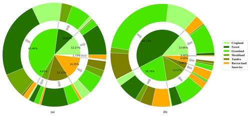
Figure 12 Land cover conversions with significant land cover change (LCC) between 1982 and 2015. The inner pie in (a) shows the percentages of different gross gain for each land cover, and the outer ring indicates which land cover the gross gain came from. The inner pie in (b) shows the percentage of different gross loss for each land cover, and the outer ring indicates which land cover the gross loss went to.

Among land converted to cropland in 2015, grassland was the biggest source (Fig. 12b), accounting for 67.58 %. A total of 6.61 % of cropland was converted from forest (Fig. 12b), showing the process of forest destruction. Among land converted to forest, the proportion of cropland reached 21.74 % (Fig. 12b). Barren land and grassland were, respectively, the largest sources of grassland and barren land, (Fig. 12b), reflecting the dynamic transformation between the two classes. Grassland accounted for 35.00 % of the increasing source of barren land (Fig. 12b), indicating the process of grassland loss (Bai et al., 2008).

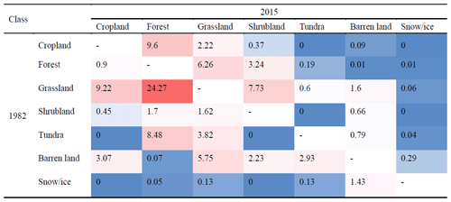
Table 13 Area ratio (%) of land cover conversions from 1982 to 2015, where the red color denotes a higher ratio and the blue color represents a lower ratio.

The most frequent direction of conversion from cropland in 1982 was forest (Fig. 12a), which reached 78.22 %. At the same time, forest was also the main cause of loss of grassland and shrubland (Fig. 12a). The conversion of forest to grassland accounted for 59.04 % of all conversions from forest (Fig. 12a). The main conversion direction of tundra was forest, reaching 64.60 % (Fig. 12a).

Overall, the increase in forest accounted for the highest proportion of all conversion processes, reaching 44.17 % (Table 13). The increases in grassland and cropland were the second and third highest, reaching 19.79 % and 13.64 %, respectively (Table 13). In addition, the proportions of grassland to shrubland and barren land to grassland were 7.73 % and 5.75 %, respectively (Table 13). Cropland gain and vegetation gain were the main phenomena reflected by the changes in global LC from 1982 to 2015.

3.4 Human impact evaluation

Figure 13a shows different human impact (HI) levels among different LCC areas. Overall, the average HI level in regions with significant changes in all LC classes is 25.49 %, indicating that human activity has a great impact on LCC. The highest HI level was found in those regions with significant increases in cropland, reaching an average value of 51.38 %. Meanwhile, the HI level of cropland loss reached 48.02 %, while the HI level for forest loss was 26.91 %. In addition, in any change of vegetation, such as forest, grassland, and shrubland, the HI level in regions of vegetation loss is higher than that of gain.

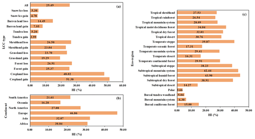
Figure 13 The mean human impact (HI) of regions with significant land cover change on the scale of (a) LCC, (b) continents, and (c) eco-regions.

The HI levels along continents can be found in Fig. 13b. The highest level of HI is found in Europe and the lowest in Oceania. The HI in Europe reached 46.86 %, indicating that human activity played a relatively important role in regions with significant LCC. Asia came second, with a HI level of 32.07 %. In South America and Oceania in the Southern Hemisphere, the overall HI level in the LCC regions is small.

As shown in Fig. 13c, the polar regions and the boreal conifer forest regions at high northern latitudes with significant LCC have lower HI levels. The level of HI in subtropical regions is high, among which HI levels in subtropical steppe and subtropical humid forest regions reached 38.23 % and 43.90 %, indicating that the role of LC conversion caused by human activity in subtropical climate areas is significant. In addition, in the temperate steppe regions, the HI level in the regions of significant LCC is also high, reaching 39.87 %. In the tropics, the average HI level in dry forest regions is highest among regions of significant LCC, reaching 34.04 %.

3.5 Local hotspots of LCC

Regarding LC, more attention tends to be paid to global and regional LCC. At the local scale, we can further explore the hot spots of LCC. The main regions of LCC hotspots are shown in Fig. 14, where the depth of color represents a significant change.

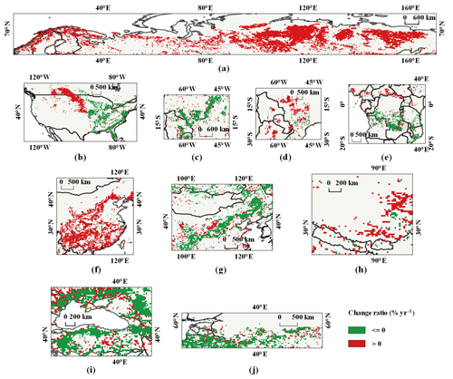
Figure 14 Visualization of local hotspots of land cover change: (a) northern Eurasia, forest; (b) Great Plains of central North America, cropland; (c) South America, forest; (d) South America, cropland; (e) Africa, forest; (f) China, forest; (g) Mongolia and Inner Mongolia (China), grassland; (h) Qinghai–Tibet Plateau, grassland; (i) central Asia, grassland; (j) the former Soviet Union in eastern Europe, cropland.

In the north of Eurasia, forest has increased significantly (Fig. 14a), and forest in Siberia has moved northward to the tundra regions. In northern North America, such as Alaska and the north of Canada, forest has also increased but the extent of the increase is weaker than that in northern Eurasia. In the Great Plains of central North America, grassland has decreased and cropland has increased (Fig. 14b). In most countries of South America, croplands have expanded substantially (Fig. 14d) and forests have decreased significantly (Fig. 14c), especially in the southeastern part of the Amazon rainforest. In Southeast Asia, such as Cambodia, Vietnam, Indonesia, and Malaysia, forest has also decreased significantly, and cropland has increased. While our LCC analysis shows these trends in the Asian tropics, higher-resolution data and more specific land cover mapping are needed to explicitly determine the reasons for LCC in this region (Cheng et al., 2018). In Africa, forest in the northern part of the Congo Basin has expanded while forest in the southern Miombo forest belt has decreased (Fig. 14e). In China, forest has increased (Fig. 14f). Some grassland in Mongolia and Inner Mongolia (China) showed a trend of decrease (Fig. 14g). There is an obvious increase in grassland areas in the eastern part of the Qinghai–Tibet Plateau (Fig. 14h) and a decrease in grassland in central Asia and parts of western Asia (Fig. 14i). In some parts of the former Soviet Union in eastern Europe, a decrease in cropland (Fig. 14j) and an increase in forest can be observed.

4 Discussion

Based on the accuracy assessment and data intercomparison results, it can be seen that the global LC mapping products of 1982–2015, GLASS-GLC, are reliable with high accuracies and that the global long-term mapping framework we designed is effective. Using GLASS-GLC CDRs in change analysis of LC can reflect a 34-year global landscape change pattern. Many phenomena and patterns can be confirmed by existing research. In addition, we have assessed the impact of human effects within different LC classes and have further explored local LCC hotspots.

However, there are still deficiencies in the design of the mapping framework. First, the large grid size of 0.05^∘ can only reflect the average change state of LC in a large area; thus, many small-area phenomena cannot be well reflected (Gómez et al., 2016). For example, the reduction of a lot of cropland is due to urbanization, and the expansion of cities is usually sporadic. Although those changes are large at the global scale, they can hardly be reflected with 0.05^∘ pixels. Moreover, due to the synthesis principle, the classification result of each pixel can only represent the class with the largest proportion in area, and the information of remaining classes is ignored even though they can sometimes be more than 50 % in total. Such a neglect, due to the famous “Scale Effect” (Turner et al., 1989) can also cause great deviations in the final statistical summary of the LC area, leading to uncertainties when compared with mapping results at finer resolutions.

Second, our sampling strategy for training has certain limitations. On the one hand, since the training sample is generated from 30 m resolution maps of more than 73 % accuracy, this will inevitably propagate and accumulate error to 5 km resolution. Of course, due to the higher signal-to-noise ratio of the high-resolution data, the sampling is still satisfactory compared to the direct visual interpretation of the coarse-resolution images. On the other hand, the training sample used is only from a single year (circa 2015). Although we have implemented a time series correction for the original input data and performed a time-consistent post processing on the classification results, the effects of interannual fluctuations in data cannot be completely avoided (X.-P. Song et al., 2018). On the other hand, according to the stable classification with limited sample theory (Gong et al., 2019), a representative sample collected in 1 year with less than 20 % in error should suffice for multiannual use at the global scale. Therefore, a multi-year sample set may not be as critical for multiannual classification provided the sample is more than 80 % accurate. In our case, although the source training data have an accuracy of 73.17 %, we are not certain if the aggregated sample set exceeds an accuracy of 80 %. While this needs further assessment, the expected loss of accuracy should be within a couple of percent (Cheng et al., 2018). According to the 92.26 % test accuracy reported in Sect. 3.1.1, the aggregated sample set can be satisfactory.

For the generation of test sample units in 2015, we have adopted the scale-up approach. That is to say, we first upscaled the 30 m test sample set to 5 km by maximum area synthesis, which contains unavoidable errors because of scale transformation. Due to the difficulty of visual interpretation in coarse-scale field investigations (Gong et al., 2013), establishing a sample library at 5 km resolution is not easy. Thus, instead, we adopted the data aggregation method based on the 30 m FROM-GLC_v2 results. Since mixed pixel problems for remotely sensed data are unavoidable at any scale, choosing one category for mixed pixels is inevitable and the cost of simplification in a traditional classification process. The development of LC ratio mapping products (similar to VCF products), rather than hard classification, especially for the case of coarse resolution, should be considered and further assessed. However, the independently interpreted 5 km test sample set alleviates the problem.

We have eliminated wetland and impervious surface in our classification system. This is a tradeoff when working at the 5 km scale. Patches of wetland and impervious surface are usually small, and it is difficult to achieve a pixel size of 0.05^∘ for many situations, so the classification of the two types is extremely difficult. However, both are important LC types. Wetland is a transitional zone between terrestrial ecosystems and aquatic ecosystems (Davidson, 2014). The impervious surface can represent the urban area. In recent years, urban expansion has been a relatively significant phenomenon in global environmental change (Seto et al., 2011). Urban expansion reflects an important type of human activity, so the impervious surface is also one of the essential components to reflect anthropogenic influence. However, the total area of its change is usually small.

It should be pointed out that at a coarse resolution of 0.05^∘, our definition of forest is more inclined to the tree canopy cover. Thus, the changes in internal density of trees can also be reflected in the area change of forest instead of just the stand-replacement type (Korhonen et al., 2006). In addition, the dominant-class synthesis strategy we adopted also makes it unavoidable to include internal density change of various classes, which in turn will further affect the classification and change area calculation of forest class.

In addition, because we are mainly depicting the natural biophysical properties of vegetated areas with limitation in resolution, some artificial characteristics cannot be distinguished, such as plantations (rubber, oil palm, and various fruit trees) and natural forest, which are uniformly included as forest in our classification system.

In the statistical analysis, although we have already conducted post-classification time-consistency processing for the original LC mapping results as much as possible, it is inevitable that there are still large fluctuations and interferences from various unknown factors unfavorable to the extraction of a long-term trend of LCC. In order to ensure that the trend of the resulting time series is significant, we have to scale up the classification result from 0.05 to 0.25^∘, converting the original class label of each 0.05^∘ pixel to the class area ratio of a 0.25^∘ grid. The long-term time series of the area ratios are tested for statistical significance. However, in some cases, this procedure will also be influenced by the “Scale Effect”.

In the analysis of anthropogenic influences, indirect effects of many human activities were ignored because the main objective was to include the effects of directly visible human activities. For example, human activities increase the concentration of carbon dioxide in the atmosphere, which in turn affects the global climate, leading to higher temperature and thus increasing vegetation coverage (Piao et al., 2006; Bonan, 2008). This pathway of action is indirect, but it is difficult to reflect in the human impact data we use, which results in an underestimation of the assessment of anthropogenic influences.

GLASS-GLCs contain more detailed LC classes, longer temporal coverage (34 years), and a high consistency product, which meets the requirement for CDR. GLASS-GLC CDRs are the first collection of global LC dynamics of 5 km and fill the existing gap for high-reliability and consistency of long-term general-purpose global LC products. In addition, our strategy of generating samples from high-resolution classification products can greatly reduce the cost and investment of sample collection. It can flexibly and effectively be extended to other coarse-resolution LC mapping tasks in the future.

In the future, with the advancement of technology and the accumulation of remote sensing data sets, the use of remote sensing products for LC mapping with higher resolution and longer time series will undoubtedly better reflect the global LC and its changes. However, under limited conditions, we can consider using coarse-resolution satellite data to determine the locations of potential rapid change and then use high-resolution data in these hotspots to accurately estimate the rate and mode of change. Moreover, it is necessary to establish a multi-year sample library to assess the impact of interannual fluctuations in input data on the accuracy of change characterization and analysis. Wetland and impervious surface are LC classes that have extremely high value. It would be useful to supplement the mapping and change analysis of these two classes when suitable data become available. For the analysis of global LCC, systematic and in-depth attribution analysis and research can be further carried out.

5 Data availability

GLASS-GLC products at 5 km resolution from 1982 to 2015 are available to the public in the GeoTIFF format at https://doi.org//10.1594/PANGAEA.913496 (Liu et al., 2020).

GLASS CDRs were provided by Beijing Normal University Data Center  (available at http://glass-product.bnu.edu.cn/, GLASS, 2018). VCF products were obtained from LP DAAC (available at https://lpdaac.usgs.gov/, NASA, 2018). GMTED2010 were acquired from the Google Earth Engine (available at https://code.earthengine.google.com/, USGS, 2018). Geo-Wiki points came from the human impact campaign (available at https://doi.org/10.1594/PANGAEA.869680, Fritz et al., 2018). Eco-region data were obtained from the FAO global eco-region data set (available at http://www.fao.org/geonetwork/srv/en/metadata.show?CurrTab=simple&id=1255, FAO, 2018).

6 Conclusions

In order to better reflect the global land changes, continuous and dynamic monitoring of global LC is necessary. We built GLASS-GLC, the first CDRs for global LC on the GEE platform. It can capture the global LCC information from 1982 to 2015. Compared to previous global LC products, GLASS-GLC products cover a longer time period and have higher consistency and more detailed classes. Our entire mapping framework is based on FROM-GLC_v2, including the classification system and high-quality H-homo sample generation.

Based on over 10 000 independent test samples units from both the FROM-GLC sample set and FLUXNET site data in 2015, the overall accuracy of GLASS-GLC was shown to exceed 80 %. With 2431 test sample units in different years, the overall accuracy of GLASS-GLC is also over 80 %, at 82.81 %. Using intercomparisons with other global LC products of different resolutions from various data sources, we verified the effectiveness and reliability of GLASS-GLC from different perspectives. Systematic uncertainty analysis was also performed on a global scale based on the results of the accuracy assessment and its geographical distribution. This shows that GLASS-GLC CDR products have relatively low uncertainty in most parts of the world. Our results also indicate that GLASS CDRs have potential for multi-class LC mapping and can provide more than enough information to distinguish different LC classes, with relatively strong temporal and spatial consistency, which can produce extremely reliable change information.

Comprehensive spatiotemporal pattern analysis based on GLASS-GLC reflected and revealed many significant global LCC phenomena and patterns, such as forest loss and cropland gain in the tropics, forest gain in the northern regions. An analysis of the global LC conversion pattern from 1982 to 2015 revealed hot spot of LCC. Since anthropogenic influence has become one of the most important driving forces for LCC, especially after the industrial revolution, we quantified the level of human impact in areas of significant LCC. The results show that the average human impact level in areas of significant LCC is about 25.49 %.

With increasing economic globalization, LCC has increased. Based on GLASS-GLC, effective global LC and change analysis could be conducted, enhancing our understanding of global environmental change, and even mitigating its negative impact to some extent, which is also beneficial to the achievement of sustainable development goals.