the Creative Commons Attribution 4.0 License.
the Creative Commons Attribution 4.0 License.
 | 28 May 2020
High-resolution (1 km) Polar WRF output for 79° N Glacier and the northeast of Greenland from 2014 to 2018
Thomas Mölg
Emily Collier
The northeast region of Greenland is of growing interest due to changes taking place on the large marine-terminating glaciers which drain the Northeast Greenland Ice Stream. Nioghalvfjerdsfjorden, or 79∘ N Glacier, is one of these that is currently experiencing accelerated thinning, retreat, and enhanced surface melt. Understanding both the influence of atmospheric processes on the glacier and feedbacks from changing surface conditions is crucial for our understanding of present stability and future change. However, relatively few studies have focused on the atmospheric processes in this region, and even fewer have used high-resolution modelling as a tool to address these research questions. Here we present a high-spatial-resolution (1 km) and high-temporal-resolution (up to hourly) atmospheric modelling dataset, NEGIS_WRF, for the 79∘ N and northeast Greenland region from 2014 to 2018 and an evaluation of the model's success at representing daily near-surface meteorology when compared with automatic weather station records. The dataset (Turton et al., 2019b: https://doi.org/10.17605/OSF.IO/53E6Z) is now available for a wide variety of applications in the atmospheric, hydrological, and oceanic sciences in the study region.
- Article
(1544 KB) - Full-text XML
- BibTeX
- EndNote


The surface mass balance of a glacier is largely controlled by regional climate through varying mass gains and losses in the ablation and accumulation zones, respectively. The large amount of mass lost from the Greenland Ice Sheet (GrIS) within the last few decades (approximately 3800 billion tonnes of ice between 1992 and 2018: Shepherd et al., 2020) has largely been located around the coast of Greenland, due to the thinning and retreat of marine-terminating glaciers (Howat and Eddy, 2011) and the surface mass loss in the ablation zone due to enhanced melting and runoff (Rignot et al., 2015; van den Broeke et al., 2017). A recent study found that enhanced meltwater runoff, connected to changing atmospheric conditions, was the largest contributor of mass loss for Greenland (52 %) (Shepherd et al., 2020). The remaining 48 % of mass loss (1.8 billion tonnes of ice) was due to enhanced glacier discharge, which has been increasing over time (Shepherd et al., 2020).
The majority of studies of the surface mass loss in Greenland and its atmospheric controls are largely constrained to southern and western Greenland (e.g. Kuipers Munneke et al., 2018; Mernild et al., 2018), or to specific warm events such as the 2012 melt event (e.g. Bennartz et al., 2013; Tedesco et al., 2013). However, recent studies have shown that the northeast of Greenland, specifically the Northeast Greenland Ice Steam (NEGIS), is now experiencing high ice velocity and accelerated thinning rates (Joughin et al., 2010; Khan et al., 2014). NEGIS extends into the interior of the Greenland ice sheet by 600 km, and three marine-terminating glaciers connect the NEGIS with the ocean. The largest of these glaciers is Nioghalvfjerdsfjorden, often named 79∘ N after its latitudinal position. Until recently, very few studies focused on 79∘ N Glacier and NEGIS as they were thought to contribute little to surface mass loss and instabilities (Khan et al., 2014; Mayer et al., 2018). However, 79∘ N Glacier, with its 80 km long by 20 km wide floating tongue, retreated by 2–3 km between 2009 and 2012, and the surface of the tongue and part of the grounded section of the glacier are now thinning at a rate of 1 m yr−1 (Khan et al., 2014; Mayer et al. 2018). The glacier is at a crucial interface between a warming ocean and a changing atmosphere. The mass loss from the floating tongue is largely attributed to basal melting due to the presence of warm (1 ∘C) ocean water in the cavity below the glacier (Wilson and Straneo, 2015; Schaffer et al., 2017; Münchow et al., 2020). However, even the grounded part of the glacier is characterized by large melt ponds and drainage systems (Philipp Hochreuther, personal communication, July 2019), suggesting that atmospheric processes may also be at play. Furthermore, atmospheric processes may be responsible for driving the warm Atlantic water under the glacier tongue, which leads to melting of the glacier base (Münchow et al., 2020). 79∘ N Glacier is of further interest because its southerly neighbour, Zachariae Isstrom, recently lost its floating tongue (Mouginot et al., 2015).
A number of studies have used atmospheric modelling as a tool to investigate the region, although they have largely been confined to short case studies (Turton et al., 2019a), focused on past climates (e.g. 45 000 years ago by Larsen et al., 2018), or targeted specific atmospheric processes (Leeson et al., 2018; Turton et al., 2019a). There are a number of atmospheric models that have been applied to the Greenland region; however these are often run at a resolution that is too coarse to resolve 79∘ N Glacier, especially its floating tongue, which can therefore be missing in many simulations. These data are usually statistically downscaled to calculate the surface mass balance of the glacier, using a digital elevation model and a shape file of the glacier. The resolution of the atmospheric models used in published studies for Greenland generally exceed 10 km: e.g. the Modèle Atmosphérique Régional (MAR) at 20 km (Fettweis et al., 2017), RACMO2 at 11 km (Noël et al., 2016), and HIRHAM5 at 25 km (Mottram et al., 2017a). Recently, there have been attempts at modelling the polar regions using non-hydrostatic regional climate models, including HARMONIE-AROME at 2 km resolution for the southwest of Greenland (Mottram et al., 2017b) and the NHM–SMAP at 5 km resolution for the whole of Greenland (Niwano et al., 2018). However, the Mottram et al. (2017b) study does not include the northeast of Greenland. Furthermore, the focus of the Niwano et al. (2018) study was to improve the surface mass balance estimates, as opposed to providing output for a more general atmospheric sense, and the model was not convection permitting. In convection-permitting models, typically for spatial resolutions higher than 5 km, convection begins to be explicitly resolved. This can enhance the representation of convection and associated precipitation, as opposed to using a convection parameterization scheme (Pal et al., 2019). As of yet, there are no very high-resolution, multi-year atmospheric datasets available for the northeast of Greenland or the wider region.
Here, we address this data gap by presenting a 5-year (2014–2018), high-resolution (1 km) atmospheric simulation using a polar-optimized atmospheric model and evaluate its skill in representing local meteorological conditions over the 79∘ N region in northeast Greenland. The dataset is named NEGIS_WRF after its location of focus and model used. As the 79∘ N region is of growing interest, these data could be beneficial for numerous other studies and applications. Indeed, current ongoing research as part of the Greenland Ice Sheet Ocean Interaction (GROCE) project (https://groce.de/, last access: 1 October 2019) uses these data for surface mass balance studies and to investigate the relationship between specific atmospheric processes and surface melt patterns. For studies of the surface mass balance of the NEGIS, further downscaling would not be necessary. With a horizontal resolution of less than 5 km, many atmospheric processes are accurately resolved, including katabatic winds and warm-air advection (Turton et al., 2019a). Furthermore, high-resolution output is crucial for the complex topography on the northeast coast, where steep and variable topography can channel or block the winds and lead to strong variability of the radiation budget. The WRF dataset is also intended as input to an ocean model, an ocean–glacier interaction study, a hydrologic model, and an ice sheet modelling study. Here we present an evaluation of the ability of NEGIS_WRF to represent key near-surface meteorological and radiative conditions, to demonstrate the applicability of the dataset for these and other studies in the atmospheric, cryospheric, and oceanic fields.
2.1 Model configuration
The Polar Weather Research and Forecasting (Polar WRF) model is a version of the WRF model that was developed and optimized for use in polar climates (Hines et al., 2011). The non-hydrostatic WRF model (available at http://www.mmm.ucar.edu/weather-research-and-forecasting-model; last access: 29 July 2019, NCAR, 2019) has been widely used for both operational studies and for research in many regions, and at many scales (Powers et al., 2017; Skamarock and Klemp, 2008). The current version of polar WRF used here is v3.9.1.1, which was released in January 2018 and is available from http://polarmet.osu.edu/PWRF/ (last access: 29 July 2019, Ohio State University, 2019). Polar WRF has been developed for use in the Arctic and Antarctic by largely optimizing the Noah land surface model (LSM) (Chen and Dudhia, 2001) to improve heat transfer processes through snow and permanent ice, and by providing additional methods for sea ice treatment (Hines et al., 2015). For a full description of the Polar WRF additions, see Hines and Bromwich (2008) and Hines et al. (2011, 2015) and citations therein.
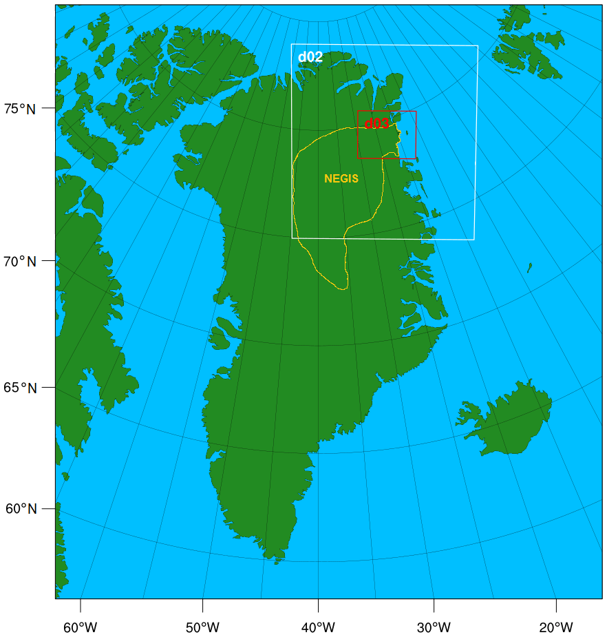
Figure 1The domain configuration for the Polar WRF runs and the approximate outline of NEGIS following Khan et al. (2014).
The meteorological initialization and boundary input data are from the ECMWF (European Centre for Medium-Range Weather Forecasts) ERA-Interim dataset at 6-hourly intervals (Dee et al., 2011). This reanalysis product was more accurate at resolving mesoscale processes in the northeast of Greenland compared to MERRA2 reanalysis data and has previously been used for Polar WRF simulations in Greenland (DuVivier and Cassano, 2013; Turton et al., 2019a). The sea surface temperature (SST) and sea ice concentration values are from the NOAA Optimum Interpolation 0.25∘ resolution daily data. This is a combination of data from the Advanced Very High Resolution Radiometer (AVHRR) infrared satellite and Advanced Microwave Scanning Radiometer (AMSR) (https://doi.org/10.5065/EMOT-1D34, NCAR, 2017, last access: 29 July 2019). In situ ship and buoy data are used to correct satellite biases, leading to relatively low mean biases of 0.2–0.4 K for SST data (more information on this dataset can be found in Banzon et al., 2016). This higher-resolution dataset was required due to the very blocky coastline in the SST and sea ice data from ERA-Interim. The domain setup is shown in Fig. 1. The outermost domain (D01) is at 25 km, D02 is 5 km, and D03 (innermost) is 1 km grid spacing. Boundary conditions, including sea ice fraction and SST, were updated every 6 h. Analysis nudging was used in the outer domain (D01) to constrain the large-scale circulation while allowing the model to freely simulate in D02 and D03. Nudging is the process of constraining the interior of model domains towards the larger-scale field (from reanalysis data) which drives the simulation (Lo et al., 2008; Otte et al., 2012). It has been found to improve simulations of the large-scale circulation (Bowden et al., 2012) and reduce errors in the mean and extreme values (Otte et al., 2012) from relatively long runs. We only nudge the outer domain (D01) to allow the higher-resolution domain to evolve freely. The USGS 24 category land use and land mask was adjusted using the European Space Agency (ESA) Climate Change Initiative (CCI) land use product, to provide a better representation of the glacier outlines and the terminus of the floating tongue (https://www.esa-landcover-cci.org/, last access: 5 September 2019, European Space Agency, 2019). A number of open-water grid points were manually changed to glacierized during January–June and September–December to better represent the floating tongue of the Spalte Glacier (tributary of 79∘ N on the northeast side) and the sea ice in the adjacent Dijmphna Sound (Fig. 2). Other small exposed water areas along the coast, which are permanently frozen except in July and August each year (Philipp Hochreuther, personal communication, July 2019), were also changed to ice during all months except July and August (Fig. 2). The glacier extents are treated as static throughout the run, which is an appropriate approximation given the small and likely negligible area of calving of 79∘ N during our study period (see ENVEO, 2019, for calving front locations from 1990 to 2017). There are 60 levels in the vertical, with a 10 hPa model top and a lowest model level ∼ 16 m above the surface.
Many of the parameterizations for the model configuration were selected based on numerous previous Polar WRF runs over Greenland and the Arctic (for example Hines et al., 2011). In brief, the following parameterizations were employed: the Noah LSM (Chen and Dudhia, 2001), due to its optimizations that have been tested over Greenland (Hines and Bromwich, 2008), Arctic sea ice (Hines et al., 2015), and Arctic land (Hines et al., 2011); the Morrison two-moment scheme for microphysics, which has been shown to out-perform other schemes in both polar regions (Bromwich et al., 2009; Lachlan-Cope et al., 2016; Listowski and Lachlan-Cope, 2017); the Eta similarity scheme for surface layer physics (Janjić, 1994); and the Yonsei University Scheme for planetary boundary layer parameterization. This was used due to the topographic wind scheme (Hong et al., 2006) that can correct excessive wind speeds in areas of complex topography, such as the northeast coast of Greenland (employed in D02 and D03 only, where complex orography is best resolved). Further parameterizations include the Kain–Fritsch scheme for cumulus convection (Kain, 2004) (D01 and D02 only, as the resolution of D03 allows convection to be explicitly resolved) and the Rapid Radiative Transfer Model (RRTM) longwave and Goddard shortwave schemes for radiation, based on sensitivity testing for the polar regions by Hines et al. (2008) and subsequent runs over Greenland (DuVivier and Cassano, 2013; Hines et al., 2011). Whilst the majority of these options were selected for testing based on the works of other publications, a short sensitivity study was also conducted, alongside testing the horizontal and vertical resolution and locations of the domains (not included). It was found that a combination of the options above were best suited to the northeast of Greenland when compared with observations on the floating tongue of 79∘ N Glacier from 1996 to 1999 (Turton et al., 2019a).
Other options specified for this study include using a fractional sea ice treatment, which allows calculation of different surface temperature, surface roughness, and turbulent fluxes for open water and sea ice conditions within the grid cell and then calculates an area-weighted average for the grid (DuVivier and Cassano, 2013; Hines et al., 2011). The adaptive time step was used to optimize the simulation speed. For each year simulated, the model was initialized on 1 September before the onset of the accumulation season and ran continuously until 1 October of the following year (e.g. 1 September 2016–1 October 2017). September was then discarded as a spin-up month. The model produces similar-magnitude snow depths to available observations (Pedersen et al., 2016). Due to limited snowfall and snow depth observations in this region, we compared cumulative snowfall to ERA5 products during testing, which have been shown to have a relatively good agreement with observations by Wang et al. (2019). The maximum snow depth and average annual accumulation were well captured by Polar WRF compared to ERA5.
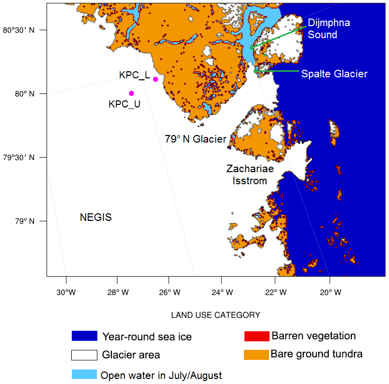
Figure 2A map of the land use types for D03. Colours represent the land use type, except for light blue, which highlights the manually changed land use from open water to sea ice during winter. Important locations are also highlighted, as are the locations of the two AWS sites (pink dots).
The data were output at hourly intervals for D03, at 6-hourly intervals for D02, and at daily intervals for D01. Daily mean values for key meteorological variables from D02 and D03 were calculated from the hourly values and are available along with the daily instantaneous values from D01 at the Open Science Framework repository (Turton et al., 2019b: https://doi.org/10.17605/OSF.IO/53E6Z).
2.2 Observational data
The remote nature of the location of interest provides few in situ observational datasets for model evaluation. However, the PROMICE (Programme for Monitoring of the Greenland Ice Sheet) network (http://www.promice.dk/, last access: 1 October 2019; van As and Fausto, 2011), operated by the Geological Survey of Denmark and Greenland (GEUS), has two permanent automatic weather stations (AWSs) available for comparison of daily means of meteorological variables and a number of surface energy balance components. The AWSs are referred to as KPC_L and KPC_U due to their location on Kronprins Christian Land (KPC, located to the northwest of 79∘ N Glacier; see Table 1 for AWS details of location, dates, and available variables). Although hourly data are available, daily means are used for evaluation due to the multi-year timescale of the study, but the authors note that an evaluation of hourly data should be performed before using these data for analysis at these timescales. Please refer to van As and Fausto (2011) and Turton et al. (2019a) for more information on the PROMICE data in this location (https://doi.org/10.22008/promice/data/aws, Fausto and van As, 2019, available at http://www.promice.dk/, last access: 1 October 2019). Observations are not taken at exactly 2 m above the surface but vary with accumulation and ablation. Over bare ice, the sensor is 2.6 m above the surface (van As and Fausto, 2011). To clarify that the observations represent near-surface conditions, and are compared with 2 and 10 m model output, we use the abbreviation X2 or X10 to represent both modelled and observed variables at the respective heights. The mean values from the observational data are calculated from daily averages from 1 January 2014 to 31 December 2018 to keep a consistent period across all data.
Table 1The location, elevation, and data availability of the two AWSs used for model evaluation. We evaluate the model output with six variables from the AWSs. Data were unavailable at KPC_L between 15 January 2010 and 17 July 2012 due to retrieval problems. T is air temperature, Q is specific humidity, and WS and WD are wind speed and direction. Observations are taken at approximately 2 m above the surface, but this does vary with accumulation and ablation (see Sect. 2.2). Sensor error estimates come from the sensor manufacturers. See van As and Fausto (2011) for more information on sensors and observations.

The in situ AWS observational data are used to evaluate the NEGIS_WRF output and to provide a judgement of its skill to benefit future users. The focus of the evaluation is to test WRF's ability to represent local meteorological conditions over a polar glacier. Daily mean values from NEGIS_WRF have been calculated from hourly output at the location of the two AWSs. All evaluation focuses on near-surface meteorological output from D03.

Figure 3The observed (black lines) and modelled (dashed blue lines) daily average air temperature at KPC_L (a) and KPC_U (b) from D03.

Figure 4The 2 m air temperature (colours), wind vectors (arrows), and terrain height contours (black lines) for 6 June 2015. The edge of 79∘ N Glacier is shown by the dark grey line.
Table 2Comparison of the near-surface WRF model output to AWS data at KPC_L and KPC_U. ANN refers to annual mean values, and DJF refers to winter average values whereas JJA refers to summer average values. Asterisks refer to statistically significant differences between WRF and AWS at the 99 % confidence interval, using Student's t test.

3.1 Model evaluation: daily means
The air temperature is simulated well by the WRF simulations with a coefficient of determination (R2) of 0.92 at both KPC_L and KPC_U (Table 2, Fig. 3). Similarly, the mean biases and RMSE are small. The mean bias and RMSE are slightly larger during winter (DJF) at KPC_U, but overall the R2 value at both locations remains above 0.64. The particularly low daily temperatures observed during winter at KPC_U are not fully captured by the WRF simulations (Fig. 3b). The model can, however, capture the larger variability in winter (Fig. 3), including “warm-air events”, where the air temperature increases by more than 10 ∘C in a few days, leading to temperatures above the average for winter (Turton et al., 2019a). Figure 4 presents the near-surface air temperature and 10 m wind vectors for 6 June 2015, to show what the temperature and wind fields look like for an example time period during the ablation period (June–August). The onset of the ablation season is earlier over the floating tongue of the glacier, as seen by the above-freezing air temperatures at low elevations in Fig. 4. WRF simulates the humidity very well annually and during winter for both locations. The humidity during summer is slightly less well simulated, with mean biases of 0.4 and 0.6 g kg−1 for KPC_L and KPC_U, respectively (Table 2).
However, the R2 values remain above 0.44 for the summer season. For both locations, annually and seasonally, WRF is moister than in observations; however the mean biases remain relatively small (less than 0.6 g kg−1), and the differences are not statistically significant except for during summer at KPC_U (which is statistically different at the 99 % confidence level using Student's t test). The wind direction in WRF deviates more from the AWS data than for temperature and moisture, which is likely due to the particularly steep and complex topography of the region which may not be accurately represented by the model, even at 1 km resolution. The largest bias is an annual bias at KPC_L (10.7∘) as WRF simulates the wind direction predominantly more northerly than in observations (Table 2), which leads to poor R2 values (0.01) and high RMSE. For KPC_U annually and seasonally, the biases remain at or below 8.6∘ and R2 values are 0.36, which shows that WRF is capable of representing the wind direction at KPC_U. Some of these errors may relate to measurement errors of the wind sensor, which is ±3∘ (see Table 1). The model performs better at simulating the wind speed than the wind direction. Annually and during winter, the R2 values are relatively high (above 0.31) at both locations, and mean biases remain at or below 2.3 m s−1 both annually and seasonally. None of the biases between WRF and observations are statistically significantly different for daily mean wind speed or air temperature (Table 2).
Shortwave and longwave radiation values are important for a range of possible future studies including input to surface mass balance and ocean models. Therefore, we have validated the NEGIS_WRF output for both the downwelling shortwave and longwave radiation by comparing it to observations at the two sites (Table 2). Annually, the biases are within sensor error range (Table 1), and differences between WRF and observations are not statistically significant for both downwelling shortwave (SWdown) and longwave (LWdown) radiation. Due to the lack of sunlight during winter at this latitude, the SWdown biases and RMSE are small and the R2 values (0.78 and 0.75 for KPC_L and KPC_U, respectively) are high for both locations (Table 2). The mean biases are largest for SWdown during summer, but a relatively high R2 value shows that WRF still has a great deal of skill (0.82 at KPC_U). Biases for LWdown are largest during winter (−10.3 and −15.3 W m−2 at KPC_L and KPC_U, respectively), which is likely a product of increased wintertime variability due to storm frequency and location (van As et al., 2009). Similarly, Cho et al. (2020) found that biases of LWdown values compared to satellite observations were larger for the Morrison microphysics scheme (which we use here) than for the WRF single-moment six-class scheme. However, it was concluded that Polar WRF has the ability to accurately simulate the spatial distribution of Arctic clouds and their optical properties with both tested schemes (Cho et al., 2020). None of the differences between WRF output and observations for the radiation components were statistically significant (Table 2).
The larger RMSE and lower R2 values during summer for wind direction can, at least partly, be attributed to the larger variability of those variables during summer. In summer (JJA), the average deviation of wind direction in observations at KPC_L is 40.3∘. Whilst WRF is able to capture this variability in wind direction (the average deviation is 41.1∘), there is sometimes an offset in the timing of the wind direction change between WRF and observations. For example, after 2 weeks of consistently northwesterly winds being observed at KPC_L between 11 and 24 August 2014, there was a shift to northeasterly flow on the morning of 25 August 2014 (Fig. 5e). WRF successfully simulated the long period of northwesterly winds, and the shift to winds from the northeast; however the change in direction was simulated in the late evening of 25 August to early morning of 26 August (Fig. 5f), leading to a bias of 156.9∘ on 25 August. The northeasterly wind was only observed for 24 h before returning to westerly on 26 August (Fig. 5g). WRF was able to capture the short-lived timing of the event, but 24 h later. In this particular case, the wind direction error comes from the boundary data, ERA-Interim. In ERA-Interim, the wind direction change starts on 24 August but remains northerly until 18:00 UTC on 25 August. It then remains northeasterly until 27 August, which is 24 h longer than in near-surface observations. The later onset and more persistent flow from the northeast in ERA-Interim likely led to the later onset of northeasterly flow in WRF. Therefore, WRF can capture both the predominant wind flow and abrupt changes to the wind direction, along with capturing even short-lived events, although the timing is occasionally shifted. Figure 5 also highlights that whilst the annual mean bias for wind speed is less than 1.5 m s−1 (Table 2), during certain periods, WRF simulates higher wind speeds than observed. However, these are not unrealistic values for this region, with a maximum observed wind speed of 20.2 m s−1 and a maximum simulated wind speed of 22.3 m s−1 for the KPC location. The largest values and biases of wind speed occur during particularly strong katabatic events (northwesterly wind direction during winter). This was also found by Hines and Bromwich (2008) when using the same land surface scheme as in these simulations.
Overall, WRF performs well at simulating air temperature, humidity, downwelling radiation, and wind speed during the simulation period (October 2013–December 2018). WRF struggles to accurately represent the wind direction, especially at KPC_L (which is likely due to the proximity of complex topography to the KPC_L site); however the winds remain predominantly westerly to northwesterly, which shows that WRF can capture the dominant katabatic process governing the wind directions.
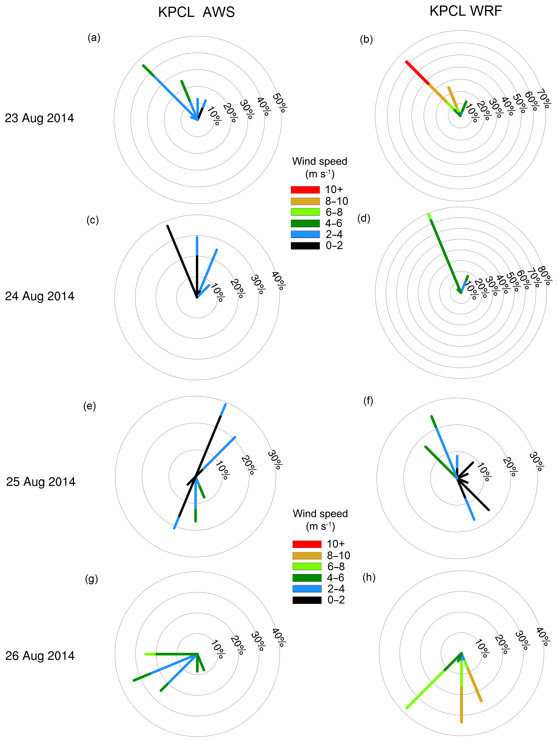
Figure 5Wind speed (colour) and direction (lines) for 23 to 26 August 2014, from observations (a, c, e, g) and WRF (b, d, f, h) at the KPC_L location. The circles (and therefore length of the spikes) represent the frequency of the particular wind direction, with the percentage of occurrence written on the circles.
3.2 Model evaluation: sub-daily data
To evaluate the ability of the model to simulate sub-daily values, the minimum and maximum daily near-surface values (from hourly output) are compared to observations, and the amplitude of the diurnal cycle of air temperature is also evaluated. Figure 6 presents the statistics for daily minimum and maximum air temperatures at the two locations in observations and WRF. The median values are well captured by WRF, especially for the maximum daily values, where a median value of −13.9 ∘C is observed at KPC_U, and −14.0 ∘C is simulated. Similarly, for maximum temperatures, the 75th quartile values are well captured by WRF (Fig. 6). For KPC_L, the minimum and maximum temperatures are colder in WRF than in observations. For example, the 25th percentile value for the minimum temperatures (far left bar in Fig. 6) is 3.8 ∘C in observations, but 6.3 ∘C in WRF. At KPC_U, the opposite is true, where WRF simulates slightly higher temperatures than in observations. However, overall, the range of minimum and maximum temperature values is well modelled by WRF.
The average daily maximum air temperature observed at KPC_L is −21.0 ∘C in winter (DJF) and increases to 3.0 ∘C in summer (JJA). WRF simulates an average daily maximum of −20.9 ∘C in winter, which increases to 0.9 ∘C in summer. The average daily minimum air temperature observed at KPC_L is −25.9 ∘C during winter and rises to 0.2 ∘C in summer. WRF simulates an average daily minimum air temperature of −26.5 ∘C in winter and increasing to −2.3 ∘C in summer. Therefore, WRF is able to accurately simulate the winter minimum and maximum temperatures. WRF slightly underestimates the air temperature during summer. However at KPC_U, this is within the error estimate provided by the sensor manufacturer (Table 1), and for both locations the biases are not statistically significant (Table 2).
Similarly, at KPC_U, the observed maximum temperature values are −24.1 ∘C in winter and 0.1 ∘C in summer. From WRF, the average maximum temperature is −22.5 ∘C in winter and increases to −0.1 ∘C in summer. The observed minimum daily air temperature at KPC_U is −30.8 ∘C during winter and −3.5 ∘C in summer. In comparison, in the WRF simulations, the average daily minimum temperature is −27.4 ∘C during winter and increases to −3.9 ∘C in summer. WRF can therefore represent the maximum and minimum daily air temperatures at KPC_U.
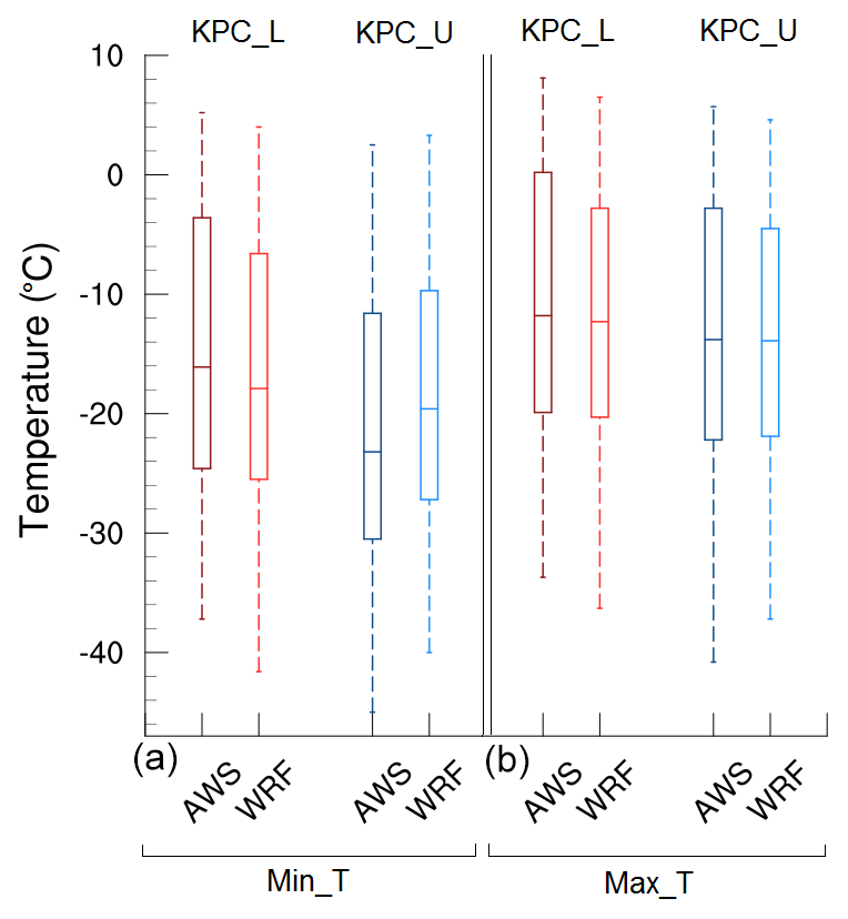
Figure 6Box plot representing the minimum (a) and maximum (b) daily temperature values at the KPC_L (red) and KPC_U (blue) locations, from both observations (darker colours) and WRF (lighter colours).
The annual-average observed diurnal air temperature amplitude is 5.6 ∘C at KPC_U and 4.0 ∘C at KPC_L. The largest average diurnal cycle is observed during spring (MAM) at KPC_U (6.8 ∘C) and during winter at KPC_L (4.9 ∘C). The WRF model simulated an average diurnal amplitude of 5.0 ∘C at KPC_U and 4.7 ∘C at KPC_L. The largest diurnal cycles are simulated during spring at KPC_U (6.2 ∘C) and during winter at KPC_L (5.5 ∘C). Therefore, WRF accurately simulates the timing of the largest diurnal amplitudes but overestimates the amplitude slightly at KPC_L and underestimates it at KPC_U, both by 0.6 ∘C. The relatively large diurnal amplitude in winter may be counterintuitive given that the glacier is located in the Arctic, where polar night (no solar radiation) prevails throughout winter. However, the temperature variability is largest during winter over the glacier due to the more frequent passing of storms across the Atlantic Ocean and the occurrence of warm-air events from easterly horizontal advection and increased longwave radiation from clouds (van As et al., 2009; Turton et al. 2019a). Warm-air events are characterized by large (> 10 ∘C) temperature increases between November and March, which can last for a number of days and, on average, occur 10 times per year (standard deviation of 4.0) (Turton et al., 2019a). The variability can be further enhanced by turbulent mixing from katabatic winds and the presence of föhn winds (Turton et al., 2019a).
The maximum hourly air temperature over the 4 years of data observed at KPC_L was on 23 July 2014 (8.1 ∘C) (Fig. 6). WRF was able to replicate the processes responsible for the particularly warm day, as a daily maximum value of 4.5 ∘C was modelled at KPC_U. At KPC_L, the maximum was simulated 24 h earlier (6.5 ∘C). The maximum values from WRF are slightly lower than observed (Fig. 6), but the timing of the maximum was accurate. The lower maximum values are likely linked to the negative mean bias in temperature simulated by WRF during the summer months (Table 2).
The absolute minimum hourly air temperature was observed at KPC_U on 26 December 2015 (−45.0 ∘C) (Fig. 6) and on 27 December 2015 at KPC (−37.2 ∘C). Again, WRF was able to capture the events leading to the particularly cold December 2015 period. On 27 December, the simulated minimum air temperature was −37.7 ∘C at KPC_L and −37.8 ∘C at KPC_U. The minimum daily values are warmer than those observed at KPC_U, but very similar to those observed at KPC_L. (Table 2).
For the first time, the atmospheric dataset NEGIS_WRF resolves the meteorological conditions over the northeast region of Greenland (5 km) and 79∘ N Glacier region at the kilometre scale over a period of 5 years (2014–2018). More than 50 variables are available (near the surface and at 60 atmospheric levels) at up to hourly temporal resolution (for the 1 km domain), including meteorological and radiative fields. Daily mean values for near-surface temperature (2 m), specific humidity (2 m), skin temperature, and U and V wind components (10 m) are available online (Turton et al., 2019b: https://doi.org/10.17605/OSF.IO/53E6Z) for the 1 and 5 km domains from 2014 to 2018. As the output frequency from D01 (25 km resolution) was once per day, the available values are instantaneous daily values at 00:00 UTC, as opposed to daily means. Furthermore, 4-D variables of temperature, humidity, U and V wind components, geopotential and pressure are available on model levels at the same frequency as the near-surface variables. For other variables, or more frequent output, please contact the lead author, and these can be made available. Due to the large amount of data, these are not stored online, but at the Regional Computation Centre Erlangen (RRZE) in Germany.
Polar WRF has previously been extensively used in the Arctic (e.g. Hines et al., 2011; Hines and Bromwich, 2017; Wilson et al., 2011), including for Greenland (e.g. DuVivier and Cassano, 2013; Turton et al., 2019a), for a number of applications. However, WRF runs have often been used for short case studies or performed at lower spatial resolution. This dataset provides high-spatial- and high-temporal-resolution runs over multiple years (2014–2018) for an area of increased interest. Regardless of the regular use of Polar WRF, it remains important to validate the model for specific locations, especially when downscaling to very high resolutions.
Overall, the mean biases are small and statistically insignificant between the Polar WRF runs and the PROMICE observations at both the lower and upper stations near 79∘ N Glacier. The R2 values are high for air temperature, humidity, and wind speed, but less so for wind direction at KPC_L. The wind direction is more variable in summer than in other months, and whilst WRF is able to simulate the increased variability, large biases can arise due to inconsistent timing of wind direction changes between WRF and observations over short periods of 24 h or less. However, as WRF is able to replicate the short-lived events and the predominant northwesterly winds of katabatic origin, we can conclude that the NEGIS_WRF can be used for further studies of the near-surface meteorology of 79∘ N Glacier. This dataset will be useful for many other applications in a number of fields including the atmospheric and cryospheric sciences, and as input to hydrological, ice sheet, and ocean models, subject to appropriate validation.
JVT wrote the paper, ran the WRF model, and evaluated the model against the observations. TM and EC contributed to the research concept, discussion, optimization of the simulations, and manuscript refinement.
The authors declare that they have no conflict of interest.
We thank Dirk van As from GEUS for his assistance with the PROMICE data and Keith Hines for the Polar WRF code. The authors also thank Masashi Niwano, the one anonymous reviewer, and Yasuhiro Murayama for improving and editing our manuscript. We acknowledge the High Performance Computing Centre (HPC) at the University of Erlangen–Nuremberg's Regional Computation Centre (RRZE), for their support and resources whilst running the Polar WRF simulations.
This research has been supported by the German Federal Ministry for Education and Research (BMBF) (grant no. 03F0778F).
This paper was edited by Kirsten Elger and reviewed by Masashi Niwano and one anonymous referee.
Banzon, V., Smith, T. M., Chin, T. M., Liu, C., and Hankins, W.: A long-term record of blended satellite and in situ sea-surface temperature for climate monitoring, modeling and environmental studies, Earth Syst. Sci. Data, 8, 165–176, https://doi.org/10.5194/essd-8-165-2016, 2016.
Bennartz, R., Shupe, M. D., Turner, D. D., Walden, V. P., Steffen, K., Cox, C. J., Kulie, M. S., Miller, B. B., and Pettersen, C.: July 2012 Greenland melt extent enhanced by low-level liquid clouds, Nature, 496, 83–86, https://doi.org/10.1038/nature12002, 2013.
Bowden, J. H., Nolte, C. G., and Otte, T. L: Simulating the impact of the large-scale circulation on the 2-m temperature and precipitation climatology, Clim. Dynam., 40, 1903–1920, https://doi.org/10.1007/s00382-012-1440-y, 2012.
Bromwich, D. H., Hines, K. M., and Bai, L.: Development and testing of Polar Weather Research and Forecasting model: 2. Arctic Ocean, J. Geophys. Res., 114, D08122, https://doi.org/10.1029/2008JD010300, 2009.
Chen, F. and Dudhia, J.: Coupling an advanced land surface-hydrology model with the Penn State-NCAR MM5 modeling system. Part 1: Model implementation and sensitivity, Mon. Weather Rev., 129, 569–585, https://doi.org/10.1175/15200493(2001)129<0569:CAALSH>2.0.CO;2, 2001.
Cho, H., Jun, S.-Y., Ho, C.-H., and McFarquhar, G.: Simulations of winter Arctic clouds and associated radiation fluces using different cloud microphysics schemes in the Polar WRF: Comparisons with CloudSat, CALIPSO and CERES, J. Geophys. Res.-Atmos., 125, e2019JD031413, https://doi.org/10.1029/2019JD031413, 2020.
Dee, D. P., Uppala, S. M., Simmons, A. J., Berrisford, P., Poli, P., Kobayashi, S., Andrae, U., Balmaseda, M. A., Balsamo, G., Bauer, P., Bechtold, P., Beljaars, A. C. M., van de Berg, I., Biblot, J., Bormann, N., Delsol, C., Dragani, R., Fuentes, M., Greer, A. J., Haimberger, L., Healy, S. B., Hersbach, H., Holm, E. V., Isaksen, L., Kallberg, P., Kohler, M., Matricardi, M., McNally, A. P., Mong-Sanz, B. M., Morcette, J.-J., Park, B.-K., Peubey, C., de Rosnay, P., Tavolato, C., Thepaut, J. N., and Vitart, F.: The ERA-Interim reanalysis: Configuration and performance of the data assimilation system, Q. J. Roy. Meteorol. Soc., 137, 553–597, https://doi.org/10.1002/qj.828, 2011.
DuVivier, A. K. and Cassano, J. J.: Evaluation of WRF Model Resolution on Simulated Mesoscale Winds and Surface Fluxes near Greenland, Mon. Weather Rev., 141, 941–963, https://doi.org/10.1175/MWR-D-12-00091.1, 2013.
ENVEO: Greenland Calving Front Dataset, 1990–2017, v3.0, Greenland Ice Sheet CCI, available at: http://cryoportal.enveo.at (last access: 21 May 2020), 2019.
European Space Agency: Climate Change Initiative landuse product, available at: https://www.esalandcover-cci.org/, last access: 5 September 2019.
Fausto, R. S. and van As, D.: Programme for monitoring of the Greenland ice sheet (PROMICE): Automatic weather station data, Version: v03, Dataset, Geological Survey of Denmark and Greenland, https://doi.org/10.22008/promice/data/aws, 2019.
Fettweis, X., Box, J. E., Agosta, C., Amory, C., Kittel, C., Lang, C., van As, D., Machguth, H., and Gallée, H.: Reconstructions of the 1900–2015 Greenland ice sheet surface mass balance using the regional climate MAR model, The Cryosphere, 11, 1015–1033, https://doi.org/10.5194/tc-11-1015-2017, 2017.
Hines, K. M. and Bromwich, D. H.: Development and Testing of Polar Weather Research and Forecasting (WRF) Model. Part I: Greenland Ice Sheet Meteorology, Mon. Weather Rev., 136, 1971–1989, https://doi.org/10.1175/2007MWR2112.1, 2008.
Hines, K. M. and Bromwich, D. H: Simulation of Late Summer Arctic Clouds during ASCOS with Polar WRF, Mon. Weather Rev., 145, 521–541, https://doi.org/10.1175/MWR-D-16-0079.1, 2017.
Hines, K. M., Bromwich, D. H., Bai, L.-S., Barlage, M., and Slater, A. G.: Development and Testing of Polar WRF. Part III: Arctic Land, J. Climate, 24, 26–48, https://doi.org/10.1175/2010JCLI3460.1, 2011.
Hines, K. M., Bromwich, D. H., Bai, L., Bitz, C. M., Powers, J. G., and Manning, K. W.: Sea Ice Enhancements to Polar WRF, Mon. Weather Rev., 143, 2363–2385, https://doi.org/10.1175/MWR-D-14-00344.1, 2015.
Hong, S.-Y., Noh, Y., Dudhia, J., Hong, S.-Y., Noh, Y., and Dudhia, J.: A New Vertical Diffusion Package with an Explicit Treatment of Entrainment Processes, Mon. Weather Rev., 134, 2318–2341, https://doi.org/10.1175/MWR3199.1, 2006.
Howat, I. and Eddy, A: Multi-decadal retreat of Greenland's marine-terminating glaciers, J. Glaciology, 57, 389-396, https://doi.org/10.3189/002214311796905631, 2011.
Janjić, Z. I.: The Step-Mountain Eta Coordinate Model: Further Developments of the Convection, Viscous Sublayer, and Turbulence Closure Schemes, Mon. Weather Rev., 122, 927–945, https://doi.org/10.1175/15200493(1994)122<0927:TSMECM>2.0.CO;2, 1994.
Joughin, I., Smith, B. E., Howat, I. M., Scambos, T., and Moon, T.: Greenland flow variability from ice-sheet-wide velocity mapping, J. Glaciol., 56, 415–430, https://doi.org/10.3189/002214310792447734, 2010.
Kain, J. S: The Kain–Fritsch Convective Parameterization: An Update, J. App. Met., 43, 170–181, https://doi.org/10.1175/1520-0450(2004)043<0170:TKCPAU>2.0.CO;2, 2004.
Khan, S. A., Kjær, K. H., Bevis, M., Bamber, J. L., Wahr, J., Kjeldsen, K. K., Bjørk, A. A., Korsgaard, N. J., Stearns, L. A., van den Broeke, M. R., Liu, L., Larsen, N. K., and Muresan, I. S.: Sustained mass loss of the northeast Greenland ice sheet triggered by regional warming, Nat. Clim. Change, 4, 292–299, https://doi.org/10.1038/nclimate2161, 2014.
Kuipers Munneke, P., Smeets, C. J. P. P., Reijmer, C. H., Oerlemans, J., van de Wal., R. S. W., and van den Broeke, M. R.: The K-transect on the western Greenland Ice Sheet: Surface energy balance (2003–2016), Arct. Antarct. Alp. Res., 50, e1420952, https://doi.org/10.1080/15230430.2017.1420952, 2018.
Lachlan-Cope, T., Listowski, C., and O'Shea, S.: The microphysics of clouds over the Antarctic Peninsula – Part 1: Observations, Atmos. Chem. Phys., 16, 15605–15617, https://doi.org/10.5194/acp-16-15605-2016, 2016.
Larsen, N. K., Levy, L. B., Carlson, A. E., Buizert, C., Olsen, J., Strunk, A., Bjørk, A. A., and Skov, D. S.: Instability of the Northeast Greenland Ice Stream over the last 45,000 years, Nat. Commun., 9, 1872, https://doi.org/10.1038/s41467-018-04312-7, 2018.
Leeson, A. A., Eastoe, E., and Fettweis, X.: Extreme temperature events on Greenland in observations and the MAR regional climate model, The Cryosphere, 12, 1091–1102, https://doi.org/10.5194/tc-12-1091-2018, 2018.
Listowski, C. and Lachlan-Cope, T.: The microphysics of clouds over the Antarctic Peninsula – Part 2: modelling aspects within Polar WRF, Atmos. Chem. Phys., 17, 10195–10221, https://doi.org/10.5194/acp-17-10195-2017, 2017.
Lo, J. C.-F., Yang, Z.-L., and Pielke Sr., R. A.: Assessment of three dynamical climate downscaling methods using the Weather Research and Forecasting (WRF) model, J. Geophys. Res.-Atmos., 113, D09112, https://doi.org/10.1029/2007JD009216, 2008.
Mayer, C., Schaffer, J., Hattermann, T., Floricioiu, D., Krieger, L., Dodd, P. A., Kanzow, T., Licciulli, C., and Schannwell, C.: Large ice loss variability at Nioghalvfjerdsfjorden Glacier, Northeast Greenland, Nat. Commun., 9, 2768, https://doi.org/10.1038/s41467-018-05180-x, 2018.
Mernild, S. H., Liston, G. E., van As, D., Hasholt, B., and Yde, J. C.: High-resolution ice sheet surface mass-balance and spatiotemporal runoff simulations: Kangerlussuaq, west Greenland, Arct. Antarct. Alp. Res., 50, S100008, https://doi.org/10.1080/15230430.2017.1415856, 2018.
Mottram, R., Boberg, F., Langen, P., Yang, S., Rodehacke, C., Christensen, J., and Madsen, M.: Surface mass balance of the Greenland ice sheet in the regional climate model HIRHAM5: Present state and future prospects, Low Temp. Sci., 75, 105–115, 2017a.
Mottram, R., Nielsen, K. P., Gleeson, E., and Yang, X.: Modelling Glaciers in the HARMONIE-AROME NWP model, Adv. Sci. Res., 14, 323–334, https://doi.org/10.5194/asr-14-323-2017, 2017b.
Mouginot, J., Rignot, E., Scheuchl, B., Fenty, I., Khazendar, A., Morlighem, M., Buzzi, A., and Paden, J.: Fast retreat of Zachariæ Isstrøm, northeast Greenland, Science, 350, 1357–1361, https://doi.org/10.1126/SCIENCE.AAC7111, 2015.
Münchow, A., Schaffer, J., and Kanzow, T: Ocean circulation connecting Fram Strait to Glaciers off North-East Greenland: Mean flows, topographic Rossby waves, and their forcing, J. Phys. Oceanogr., 50, 509–530, https://doi.org/10.1175/JPO-D-19-0085.1, 2020.
NCAR: NOAA Optimum Interpolation 1/4 Degree Daily Sea Surface Temperature Analysis, Research Data Archive at the National Center for Atmospheric Research,National Centers for Environmental Information, NESDIS, NOAA, and U.S. Department of Commerce, Computational and Information Systems Laboratory, https://doi.org/10.5065/EM0T-1D34, 2007.
NCAR: Weather Research and Forecasting Model, National Centre for Atmospheric Research, available at: https://www.mmm.ucar.edu/weather-research-and forecasting-model,last access: 1 October 2019.
Niwano, M., Aoki, T., Hashimoto, A., Matoba, S., Yamaguchi, S., Tanikawa, T., Fujita, K., Tsushima, A., Iizuka, Y., Shimada, R., and Hori, M.: NHM–SMAP: spatially and temporally high-resolution nonhydrostatic atmospheric model coupled with detailed snow process model for Greenland Ice Sheet, The Cryosphere, 12, 635–655, https://doi.org/10.5194/tc-12-635-2018, 2018.
Noël, B., van de Berg, W. J., Machguth, H., Lhermitte, S., Howat, I., Fettweis, X., and van den Broeke, M. R.: A daily, 1 km resolution data set of downscaled Greenland ice sheet surface mass balance (1958–2015), The Cryosphere, 10, 2361–2377, https://doi.org/10.5194/tc-10-2361-2016, 2016.
Ohio State University: Polar Weather Research and Forecasting Model, available at: http://polarmet.osu.edu/PWRF/, last access: 29 July 2019.
Otte, T. L., Nolte, C. G., Otte, M. J., and Bowden, J. H.: Does Nudging Squelch the Extremes in Regional climate modeling?, J. Climate, 25, 7046–7066, https://doi.org/10.1175/JCLID-12-00048.1, 2012.
Pal., S., Change, H.-I., Castro, C. L., and Dominguez, F.: Credibility of convection-permitting modeling to improve seasonal precipitation forecasting in the southwestern United States, Front. Earth Sci., 7, 11, https://doi.org/10.3389/feart.2019.00011, 2019.
Pedersen, S. H., Tamstorf, M. P., Abermann, J., Westergaard-Nielsen, A., Lund, M., Skov, K., Sigsgaard, C., Mylius, M. R., Hansen, B. U., Liston, G. E., and Schmidt, N. M.: Spatiotemporal characteristics of seasonal snow cover in Northeast Greenland from in situ observations, Arct. Antarct. Alp. Res., 48, 653–671, https://doi.org/10.1657/AAAR0016-028, 2016.
Powers, J. G., Klemp, J. B., Skamarock, W. C., Davis, C. A., Dudhia, J., Gill, D. O., Coen, J. L., and Duda, M. G.: The Weather Research and Forecasting Model: Overview, System Efforts, and Future Directions, B. Am. Meteorol. Soc., 98, 1717–1737, https://doi.org/10.1175/BAMS-D-15-00308.1, 2017.
Rignot, E., Fenty, I., Xu, Y., Cai, C., and Kemp, C: Undercutting of marine-terminating glaciers in West Greenland, Geophys. Res. Lett., 42, 5909–5917, https://doi.org/10.1002/2015GL064236, 2015.
Schaffer, J., von Appen, W.-J., Dodd, P. A., Hofstede, C., Mayer, C., de Steur, L., and Kanzow, T.: Warm water pathways toward Nioghalvfjerdsfjorden Glacier, Northeast Greenland, J. Geophys. Res.-Oceans, 122, 4004–4020, https://doi.org/10.1002/2016JC012462, 2017.
Shepherd, A., Ivins, E., Rignot, E., et al.: Mass balance of the Greenland Ice Sheet from 1992 to 2018, Nature, 579, 233–239, https://doi.org/10.1038/s41586-019-1855-2, 2020.
Skamarock, W. C. and Klemp, J. B.: A time-split nonhydrostatic atmospheric model for weather research and forecasting applications. J. Computat. Phys., 227, 3465–3485, https://doi.org/10.1016/j.jcp.2007.01.037, 2008.
Tedesco, M., Fettweis, X., Mote, T., Wahr, J., Alexander, P., Box, J. E., and Wouters, B.: Evidence and analysis of 2012 Greenland records from spaceborne observations, a regional climate model and reanalysis data, The Cryosphere, 7, 615–630, https://doi.org/10.5194/tc-7-615-2013, 2013.
Turton, J. V., Mölg, T., and Van As, D.: Atmospheric Processes and Climatological Characteristics of the 79N Glacier (Northeast Greenland), Mon. Weather Rev., 147, 1375–1394, https://doi.org/10.1175/MWR-D-18-0366.1, 2019a.
Turton, J. V., Mölg, T., and Collier, E.: NEGIS_WRF model output, Open Science Framework Repository, https://doi.org/10.17605/OSF.IO/53E6Z, 2019b.
van As, D. and Fausto, R.: Programme for Monitoring of the Greenland Ice Sheet (PROMICE): first temperature and ablation records, Geolog. Survey Denmark Greenland Bulletin, 23, 73–76, 2011.
van As, D., Bøggild, C. E., Nielsen, S., Ahlstrøm, A. P., Fausto, R. S., Podlech, S., and Andersen, M. L.: Climatology and ablation at the South Greenland ice sheet margin from automatic weather station observations, The Cryosphere Discuss., 3, 117–158, https://doi.org/10.5194/tcd-3-117-2009, 2009.
van den Broeke, M., Box, J., Fettweis, X., Hanna, E., Noël, B., Tedesco, M., van As, D., van de Berg, W. J., and van Kampenhout, L.: Greenland Ice Sheet Surface Mass Loss: Recent Developments in Observation and Modeling, Curr. Clim. Change Rep., 3, 345–356, https://doi.org/10.1007/s40641-017-0084-8, 2017.
Wang, C., Graham, R. M., Wang, K., Gerland, S., and Granskog, M. A.: Comparison of ERA5 and ERA-Interim near-surface air temperature, snowfall and precipitation over Arctic sea ice: effects on sea ice thermodynamics and evolution, The Cryosphere, 13, 1661–1679, https://doi.org/10.5194/tc-13-1661-2019, 2019.
Wilson, N. J. and Straneo, F.: Water exchange between the continental shelf and the cavity beneath Nioghalvfjerdsbrae (79 North Glacier), Geophys. Res. Lett., 42, 7648–7654, https://doi.org/10.1002/2015GL064944, 2015.
Wilson, A. B., Bromwich, D. H., and Hines, K. M.: Evaluation of Polar WRF forecasts on the Arctic System Reanalysis domain: Surface and upper air analysis, J. Geophys. Res., 116, D11112, https://doi.org/10.1029/2010JD015013, 2011.