the Creative Commons Attribution 4.0 License.
the Creative Commons Attribution 4.0 License.
 | 17 May 2019
A global map of emission clumps for future monitoring of fossil fuel CO2 emissions from space
Yilong Wang
Philippe Ciais
Grégoire Broquet
François-Marie Bréon
Tomohiro Oda
Franck Lespinas
Yasjka Meijer
Armin Loescher
Greet Janssens-Maenhout
Haoran Xu
Shu Tao
Kevin R. Gurney
Geoffrey Roest
Diego Santaren
Yongxian Su
A large fraction of fossil fuel CO2 emissions emanate from “hotspots”, such as cities (where direct CO2 emissions related to fossil fuel combustion in transport, residential, commercial sectors, etc., excluding emissions from electricity-producing power plants, occur), isolated power plants, and manufacturing facilities, which cover a small fraction of the land surface. The coverage of all high-emitting cities and point sources across the globe by bottom-up inventories is far from complete, and for most of those covered, the uncertainties in CO2 emission estimates in bottom-up inventories are too large to allow continuous and rigorous assessment of emission changes (Gurney et al., 2019). Space-borne imagery of atmospheric CO2 has the potential to provide independent estimates of CO2 emissions from hotspots. But first, what a hotspot is needs to be defined for the purpose of satellite observations. The proposed space-borne imagers with global coverage planned for the coming decade have a pixel size on the order of a few square kilometers and a XCO2 accuracy and precision of <1 ppm for individual measurements of vertically integrated columns of dry-air mole fractions of CO2 (XCO2). This resolution and precision is insufficient to provide a cartography of emissions for each individual pixel. Rather, the integrated emission of diffuse emitting areas and intense point sources is sought. In this study, we characterize area and point fossil fuel CO2 emitting sources which generate coherent XCO2 plumes that may be observed from space. We characterize these emitting sources around the globe and they are referred to as “emission clumps” hereafter. An algorithm is proposed to identify emission clumps worldwide, based on the ODIAC global high-resolution 1 km fossil fuel emission data product. The clump algorithm selects the major urban areas from a GIS (geographic information system) file and two emission thresholds. The selected urban areas and a high emission threshold are used to identify clump cores such as inner city areas or large power plants. A low threshold and a random walker (RW) scheme are then used to aggregate all grid cells contiguous to cores in order to define a single clump. With our definition of the thresholds, which are appropriate for a space imagery with 0.5 ppm precision for a single XCO2 measurement, a total of 11 314 individual clumps, with 5088 area clumps, and 6226 point-source clumps (power plants) are identified. These clumps contribute 72 % of the global fossil fuel CO2 emissions according to the ODIAC inventory. The emission clumps is a new tool for comparing fossil fuel CO2 emissions from different inventories and objectively identifying emitting areas that have a potential to be detected by future global satellite imagery of XCO2. The emission clump data product is distributed from https://doi.org/10.6084/m9.figshare.7217726.v1.
- Article
(3030 KB) - Full-text XML
-
Supplement
(489 KB) - BibTeX
- EndNote


Monitoring the effectiveness of emission reductions after the Paris Agreement on Climate (UNFCCC, 2015) requires frequently updated estimates of fossil fuel CO2 emissions and a global synthesis of these estimates. The need for emission monitoring goes beyond national estimates, as many cities and regions have set concrete objectives to reduce their greenhouse gas emissions. The CO2 emissions (direct and indirect) related to final energy use in cities are estimated to be 71 % of the global total (IEA, 2008; Seto et al., 2014). In addition, power plants account for ∼40 % of direct energy-related CO2 emissions and are subject to regulations that require regular reporting of their emissions. The contribution from cities (excluding electricity-related emissions from large power plants; see Sect. 2) and power plants to national and global mitigation efforts is thus critical (Creutzig et al., 2015; Shan et al., 2018).
The technique called atmospheric CO2 inversion quantifies emissions based on a prior estimate from inventories, atmospheric CO2 measurements, and atmospheric transport models. Inversions of fossil fuel CO2 emissions have used in situ surface networks, aircraft measurements and mobile platforms around cities (Bréon et al., 2015; Lauvaux et al., 2016; Staufer et al., 2016), but the deployment of a network around each city may be impractical. Alternatively, it is possible to measure vertically integrated columns of dry-air mole fractions of CO2 (XCO2) from satellites passing over emission hotspots. Satellite measurements offer the advantage of global spatial coverage, but research studies consistently outlined that satellite XCO2 measurements need to have a high precision (<1 ppm) and a spatial sampling at high resolution (<2–3 km horizontal resolution) (Bovensmann et al., 2010; O'Brien et al., 2016). For example, the Greenhouse Gases Observing Satellite 2 (GOSAT-2) aims to measure XCO2 at 0.5 ppm precision (https://directory.eoportal.org/web/eoportal/satellite-missions/g/gosat-2, last access: 7 August 2018). The single sounding random error in XCO2 from the Orbiting Carbon Observatory 2 (OCO-2) is on the order of magnitude of 0.5 ppm (Eldering et al., 2017; Chatterjee et al., 2017). XCO2 measurements from selected 10 km wide OCO-2 tracks downwind of large power plants were used to quantify their emissions by fitting observed XCO2 plumes with Gaussian dispersion models (Nassar et al., 2017). According to Nassar et al. (2017), the uncertainties in the emissions from three selected US power plants were constrained within 1 %–17 % of reported daily emission values. The primary scientific goal of the OCO-2 mission was to estimate natural land and ocean carbon fluxes, and tracks overpassing power plants are very sporadic, given the narrow swath width and frequent clouds. In order to improve the sampling of the atmosphere, XCO2 imagers (e.g., passive spectral imagers in the short-wave infrared spectrum) are under study. The list includes the Geostationary Carbon Observatory (GeoCARB) mission (Polonsky et al., 2014), the OCO-3 instrument on board the International Space Station capable of pointing to chosen emitting areas (https://www.nasa.gov/mission_pages/station/research/experiments/2047.html, last access: 7 August 2018) and a constellation of low earth-orbiting (LEO) imagers with a swath of a few hundred kilometers planned as future operational missions within the European Copernicus Program (Ciais et al., 2015).
The ability of imaging instruments to reduce uncertainty on CO2 emissions was investigated by atmospheric inversions with pseudo data, that is, observing system simulation experiments (OSSEs), but only for case studies of limited duration. OSSEs were performed for large cities (Broquet et al., 2018; Pillai et al., 2016), single power plants (Bovensmann et al., 2010) or for a region encompassing several cities (O'Brien et al., 2016). An OSSE study with one LEO imager over Paris (Broquet et al., 2018) solved for emissions during the 6 h before a given satellite overpass. Their results showed that the uncertainty (∼25 %) in the 6 h mean emissions in the prior estimates could be reduced to less than 10 % during a few days when the wind speed is low and there is not much cloud. The results of such case studies are informative about the potential of satellite observations in quantifying fossil fuel CO2 emissions but do not systematically give information on how many hotspots and which fraction of emissions worldwide could be constrained with XCO2 imagers.
A prerequisite for assessing the capability of satellite imagers is to have a high-resolution global map of fossil fuel CO2 emissions (Gurney et al., 2019). In this study we use the ODIAC map at 30×30 arcsec (∼1 km × 1 km) (Sect. 2.1). Not all the emitting 1×1 km land grid cells of such a map will have emissions that are sufficiently intense to produce a XCO2 plume detected with a satellite (Nassar et al., 2017; Hakkarainen et al., 2016). On the other hand, a cluster of contiguous emitting grid cells will create a stronger plume than a single emitting grid cell, so that the uncertainty on the sum of emissions from a cluster could be reduced with space-borne measurements. This poses the research question of how to define those clusters of emitting pixels (called emission clumps hereafter) that will generate individual XCO2 plumes that are detectable from space. The emission clumps should include intense area sources and large isolated point sources (e.g., power plants, large factories). Using political and administrative areas of cities to define clumps does not work for this purpose because the same administrative area may contain separate large point sources or multiple hotspots forming separable plumes, as well as areas with no or little emission. The definitions of emitting areas differ among inversion studies. Broquet et al. (2018) estimated emissions from the Île de France region, while Pillai et al. (2016) defined their emitting region as an area of 100 km × 100 km around Berlin. The arbitrary choice of emitting areas across studies makes the comparison of their results difficult and is not applicable worldwide. This justifies the need for a systematic and objective definition of emission clumps that constitutes observing targets for satellites.
The algorithm for calculating emission clumps developed in this study is inspired by research on mapping urban areas and socio-demographic activities (Li and Zhou, 2017; Elvidge et al., 1997; Zhou et al., 2015; Su et al., 2015; Doll and Pachauri, 2010; Letu et al., 2010). The corresponding algorithms can be classed as classification-based or threshold-based. Classification-based algorithms use datasets such as the normalized difference vegetation index (NDVI) and the normalized difference water index (NDWI) to train a machine-learning model to classify urban and nonurban areas (Cao et al., 2009; Huang et al., 2016). Threshold-based algorithms classify urban grid cells where some continuous variables (e.g., nighttime lights) are above a given threshold (Elvidge et al., 1997; Liu and Leung, 2015; Li et al., 2015; Liu et al., 2015). In threshold-based methods, given the high spatial heterogeneity of urbanization and urban forms, efforts have been devoted to finding local optimal thresholds, such as the “light-picking” approach which finds a local nighttime background light surrounding a target grid cell (Elvidge et al., 1997), or determining local thresholds by matching local/site-based surveys and land-use/land-cover (LULC) datasets (Zhou et al., 2014).
The problem of characterizing CO2 emission clumps posed here consists of delineating all areas that have the potential to generate detectable atmospheric XCO2 plumes. “Detectable” here means that the concentration within a plume formed by a clump should be large enough compared to the surrounding background in XCO2 images of a typical spatial resolution of ≈1 km. The magnitude of a minimum detectable XCO2 enhancement in a plume (relative to the surrounding background) depends on the individual XCO2 sounding precision. Such a sounding precision should be of a similar order of magnitude worldwide, although the solar zenith angle, aerosol loads, surface albedo etc. will affect it (Buchwitz, et al., 2013). In this context, contrary to the algorithms used for mapping urban areas, common global minimum emission thresholds for land grid cells forming a clump are relevant.
Because CO2 produced by emissions is quickly dispersed by transport, XCO2 plumes sampled at a given time by a satellite image usually relate to emissions that occurred few hours before its acquisition (Broquet et al., 2018). In this study, we focus on planned LEO imagers on Sentinel missions, assuming an equator crossing time around 11:30 local time (Buchwitz et al., 2013; Broquet et al., 2018), so that XCO2 plumes sampled by these imagers are from morning emissions. Different overpass times are also possible for other satellites. For example, Equator crossing times of OCO-2 and GOSAT are 13:00–13:30 LT. Geostationary imagers may provide a better temporal coverage of the emissions; e.g., GeoCARB images are considered to sample a city multiple times within a day (O'Brien et al., 2016).
This study aims to provide a global dataset of fossil fuel CO2 emission clumps for high-resolution atmospheric inversions that will use XCO2 imager data. Such a dataset can be used for OSSE studies to compare different imagery observation concepts for constraining fossil fuel CO2 emissions at the clump scale over the whole globe. We propose an approach that combines a threshold-based and an image-processing algorithm. Section 2 describes the high-spatial-resolution global emission map on which clumps are calculated and the algorithm used to delineate the clumps worldwide. The spatial distribution and extent of the resulting clumps throughout the globe are described in Sect. 3 and are compared with clumps diagnosed by applying the same algorithm to other emission maps. Section 4 discusses the sensitivity of the resulting clumps to the precision of XCO2 measurements and future applications of this global dataset. Section 5 describes the data availability. Conclusions are drawn in Sect. 6.
2.1 Development of a high-resolution emission map of morning emissions
We use the high-spatial-resolution ( km × 1 km) global annual fossil fuel CO2 emission map for the year 2016 from the Open Source Data Inventory of Anthropogenic CO2 (ODIAC, version 2017) (Oda and Maksyutov, 2011; Oda et al., 2018) for calculating clumps. To our knowledge, it is the only emission map with global coverage and a spatial resolution high enough to match the pixel size of ≈1 km of atmospheric XCO2 imagers. We chose the year 2016, assuming that the emission spatial distributions do not change significantly from year to year. In regions with rapid urbanization rates, the emission spatial distributions may change rapidly. The analysis of such changes is out of the scope of this paper, but the clump definition can be updated consistently with the latest high-resolution emission maps for each year, using the approach presented in Sect. 2.2. The ODIAC dataset provides emissions from power plants based on the CARMA database (Carbon Monitoring and Action, http://carma.org, last access: 5 March 2018). Emissions from these point sources were spatially allocated to the exact locations from CARMA. Emissions from other sources (industrial, residential, commercial sectors, and daily land transportation) were estimated by subtracting the sum of emissions from power plants in each country from the national totals given by the Carbon Dioxide Information and Analysis Center (CDIAC) (Boden et al., 2016). Annual emissions in each country excluding power plants were spatially distributed at 30′′ spatial resolution using nighttime light fields from the Defense Meteorological Satellite Program (DMSP) satellites. ODIAC has been used in atmospheric inversions to monitor CO2 emissions from cities (Oda et al., 2018; Lauvaux et al., 2016).
To estimate morning emissions, we combined the ODIAC emission maps with the hourly profiles from the Temporal Improvements for Modeling Emissions by Scaling (TIMES) product (Nassar et al., 2013). In TIMES, the hourly profiles were provided as 24 scaling factors for each hour of the day that can be multiplied by daily average emissions to derive hourly emissions. Hourly scaling factors of TIMES were derived for residential, commercial, industrial, electricity production, and mobile on-road sectors from the bottom-up model of fossil fuel CO2 emissions Vulcan v2.0 over the US (Gurney et al., 2009) with mobile nonroad, cement manufacture, and aircraft assumed temporally constant. The TIMES dataset also gives hourly scaling factors for 19 other high-emitting countries. These profiles were weighted by the emissions fraction in each sector from EDGAR to determine hourly profiles of total CO2 emissions. The US and 19 other high-emitting countries are called “proxy” countries. Other countries in the world were assigned one of the proxy country profiles, accounting for standard international time zones and local socio-demographic patterns (e.g., time of day when people start to work, weekend defined according to different religions). The TIMES hourly profiles were derived on the national scale (assuming identical hourly profiles within a country) and then shifted by hourly offsets according to local solar time to approximate the variability related to geophysical cycles. The original TIMES hourly profiles at resolution were downscaled to the spatial resolution of ODIAC, assuming the same profiles within each grid cell. For calculating clumps based on morning emissions, we multiplied the annual mean emission rate (in g C m−2 h−1) in each grid cell of ODIAC by the average scaling factors of emissions between 06:00 and 12:00 LT. The day-to-day and month-to-month variations in the spatial distribution of fossil fuel CO2 emissions may lead to temporal variations in the spatial extent of the clumps. In this study, we define the clumps based on two thresholds (see Sect. 2.2) to ensure that the effective clumps are always within the boundaries of the clumps and that the satellite observations should provide emission estimates consistently within a year. We thus ignore the month-to-month and day-to-day variations in the emissions.
2.2 Calculation of emission clumps
The emission clumps from point sources and intense area sources in ODIAC are separated in this study. In ODIAC, the point sources only refer to power plants in the CARMA database. So in this study, we refer to sources other than power plants as area sources. Before clumps are calculated, Fig. 1 illustrates the ranked distribution of emission rates during morning hours from point sources (red) and other grid cells (blue). Excluding emissions from point sources, the maximum emission rate of emitting grid cells from area sources is 20.7 g C m−2 h−1 and most grid cells including point sources have much larger emission rates than this value. In total, 35 % of the global total emissions are from 12 433 grid cells encompassing at least one point source.

Figure 1Cumulative distribution of mean emission rates during morning hours in ODIAC for power plants (red) and area sources (blue). The y axis represents the cumulative share of global total annual emissions at each level of emission rate for a single land grid cell (x axis). The vertical dashed lines are the two thresholds used in the clump algorithm (see text).
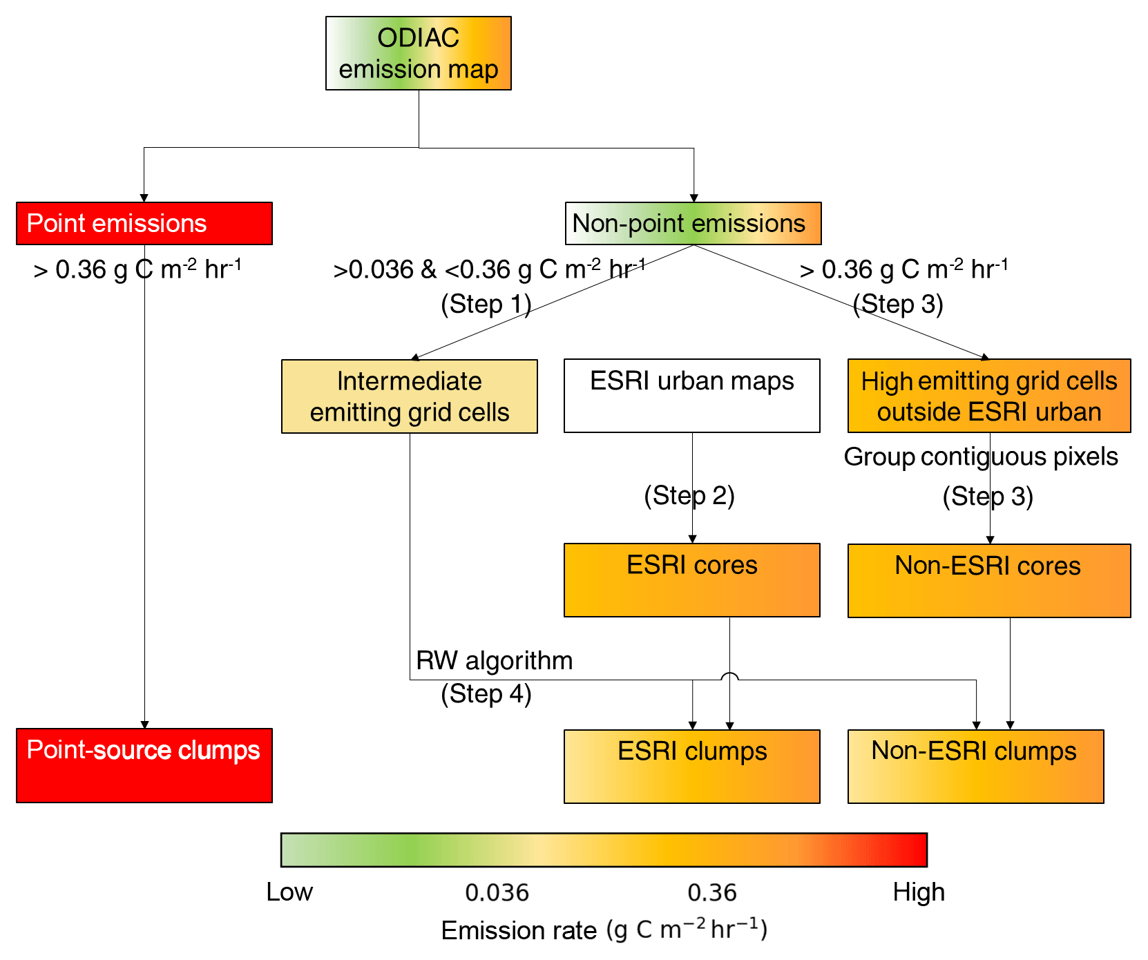
Figure 2The flow chart for calculating emission clumps. The colors qualitatively illustrate grid cell emission rates from low (light green) to high (red).
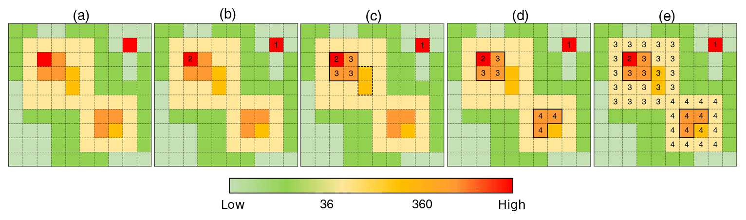
Figure 3The processes of defining emission clumps. The colors qualitatively illustrate the emission rates from low (light green) to high (red). (a) The emission field. (b) Two power plants (red grid cells) are defined as two individual clumps, labeled 1 and 2. (c) The ESRI urban area is outlined by bold solid and dashed lines, but the ESRI core is labeled 3 only for grid cells with emission rates above threshold-1. (d) The orange area represents grid cells with emissions above threshold-1 forming a non-ESRI core, labeled 4. (e) Each light-yellow grid cell is assigned to one of the clump cores using the RW algorithm (see the main text). Note that one power plant (labeled 2) is located within the ESRI urban area but is identified as a different emission clump from the ESRI clump (labeled 3 in Fig. 3e).
Figure 2 shows the flow chart of the clump algorithm. Figure 3 illustrates how it operates for a small domain as an example. Two categories of emission clumps are defined:
- a.
Only grid cells encompassing point sources with an emission rate larger than threshold-1 are considered. This threshold is chosen as 0.36 g C m−2 h−1, based on the argument that, even without any atmospheric horizontal transport, emissions lower than this threshold over 6 h would generate a local XCO2 excess of less than 0.5 ppm, the practical limit of individual sounding precision from current satellites (see Appendix for the detailed computation). This is illustrated in Fig. 3b by the red grid cell labeled 1 and 2. There are 6226 grid cells in ODIAC2017 that encompass at least one power plant and with emission rates above threshold-1, which account for >99.99 % of total emissions of all CARMA power plants globally.
- b.
Emissions clumps from area sources are calculated. We combine two data streams to calculate area clumps: (1) the administrative division of major urban areas and (2) two thresholds (threshold-1 and threshold-2 detailed below) applied to the grid cells of ODIAC. We assume that a group of emitting pixels encompassing some adjacent high-emitting pixels (forming a core of the emission clump) and their surroundings will generate an individual plume in XCO2. The urban area and the high threshold (threshold-1) define the cores of each emission clump, while threshold-2 defines the lower limit of surrounding emitting pixels to be potentially included in the clumps. The four steps to compute area sources emission clumps are detailed below.
- 1.
The value of threshold-2, above which emissions of a single emitting grid cell are selected to be potentially included in a clump, is chosen as 0.036 g C m−2 h−1, a factor of 10 lower than threshold-1. The sum of emissions from grid cells above threshold-2 represents 82 % of global total emissions (including point sources). Grid cells below threshold-2 are never included in any emission clump. Grid cells with emission rates above threshold-2 are illustrated in Fig. 3a by the yellow and orange grid cells.
- 2.
We then used the urban-area GIS (geographic information system) file from the Environmental Systems Research Institute (ESRI, https://www.arcgis.com/home/item.html?id=2853306e11b2467ba0458bf667e1c584, last access: 19 August 2017) to locate the geographic positions of major urban areas. ESRI contains 3615 separated urban areas, defined independently from the ODIAC emission map. We found 2017 ESRI urban areas containing at least one grid cell with emission above threshold-1. The remaining 1598 ESRI urban areas are not considered hereafter. An illustration of one of the 2017 selected ESRI urban areas is shown in Fig. 3c by the grid cells labeled 3. Figure 4a–c (solid lines) shows three examples of ESRI urban areas for major cities in Europe, North America, and China. The grid cells within the ESRI urban area with emission rates above threshold-1 define the cores of the clumps.
- 3.
Although the ESRI GIS file covers large cities of the world, smaller populated areas, like small cities on the southeastern coast of China that may also generate detectable plumes, are missed by the ESRI map. This calls for a complementary step to identify non-ESRI emitting clumps. For the calculation of those non-ESRI clumps, we apply threshold-1 of 0.36 g C m−2 h−1 to all grid cells that are not selected in the previous step as part of any ESRI core. Contiguous non-ESRI grid cells above threshold-1 form a non-ESRI core of clumps. These non-ESRI core grid cells must be spatially distinct from the ESRI core grid cells. If they are adjacent to any ESRI core, they are absorbed by the ESRI ones. A total of 3071 non-ESRI cores are calculated, as shown in Fig. 3d by the grid cells labeled 4.
- 4.
After ESRI and non-ESRI clump cores are defined, we aggregate all the emitting grid cells with emission rates larger than threshold-2 in their vicinity to form a clump. An ensemble of grid cells with emissions higher than threshold-2 in a domain with N cores are attributed to N distinct emission clumps. The attribution of a grid cell to a given core is calculated based on the spatial gradients of emissions and the distance between the emitting grid cells by using a random walker (RW) algorithm (Grady, 2006). RW is a type of algorithm used in the field of image segmentation, i.e., recognizing different segments or objects in a picture or photograph. The clumps with an ESRI core (step 2) are called “ESRI clumps”, while the clumps with a non-ESRI core (step 3) are called “non-ESRI clumps” hereafter. This step is illustrated in Fig. 3e by the grid cells in light yellow.
- 1.

Figure 4Emission clumps near Paris (a, d), Beijing (b, e) and New York (c, f). In panels (a)–(c), solid lines depict the urban areas from ESRI product. Colored patches depict the clump area resulting from the algorithm defined in this study. In panels (d)–(f), solid lines depict the boundaries of final clumps (boundary of colored patches in panels a–c). Colored fields in panels (d)–(f) show the emissions from the ODIAC product. Light dashed lines indicate grids.
The RW algorithm defines the probability of each grid cell to belong to some known labeled “seeds” (i.e., the cores defined in steps 2 and 3 in this study). This algorithm imagines that a random walker starts from each grid cell and is labeled (in this study, the grid cells with emissions that are above threshold-2 but not included in the cores). The probabilities that the walker will arrive at each known seed, following the easiest path, are computed. The undefined grid cells are assigned to the seed that has the highest probability of being reached by the walker. Specifically, in this study, we define the probability that the walker moves between two neighboring grid cells using an exponential decaying function of the ℓ2 norm of the log-transformed local gradients in emissions (Grady, 2006):
where wij is the probability of motion between neighboring grid cells i and j, gi and gj are image intensity (defined as the log-transformed emission rate in this study), and β is a free penalization parameter for the motion of random walker (the greater the β, the more difficult the motion). In this study, only β impacts how the undefined grid cells are assigned to the cores. It balances the effect of local gradients and the distance of the path from the undefined grid cells to the seeds: the larger the gradient along a path between the undefined grid cells and the seeds, the smaller the probability that the walker will move; and the longer the path, the smaller the probability that the walker would arrive at corresponding seeds. A larger β will lead to a larger impact of emission gradients than that of distance. In this study, , where σg is the standard deviation of the emission rates at all the grid cells in ODIAC. In general, the algorithm can effectively separate different clusters of grid cells with different spatial distributions. For instance, a clump with a flat distribution of emissions and a clump (of a similar size to the former one) with more skewed emissions are separated near the steepest gradients. This assumes that large emission gradients will generate large gradients in XCO2 (given similar meteorological condition for neighboring clumps) and that different XCO2 plumes are separable where the XCO2 gradients are the largest.
After the RW algorithm, grid cells above threshold-2 that are not contiguous to any core are discarded. This removes 10 % of the total from the 82 % of global emissions defined in step 1. As a result, 72 % of the global emissions are included in the emission clumps (see more detailed discussion below).
All the computation are made under the Python version 2.7 environment (Python Software Foundation, http://www.python.org, last access: 5 March 2018) and the RW algorithm is from package “scikit-image” version 0.14dev (http://scikit-image.org/, last access: 5 March 2018).
3.1 Emission clumps defined on ODIAC emission map
Figure 4 shows three regional clumps near Paris (France), New York (USA), and Beijing (China). The clumps near Paris are isolated from each other. There are more emission clumps in the New York region. Because some clumps are close to each other in this region (e.g., New York and Clifton), their plumes will only be distinct when the wind direction is roughly perpendicular to the direction of the line connecting clumps (i.e., from southwest to northeast or the opposite for New York and Clifton). Near Beijing, there are a larger number of clumps than in the other two regions and their distribution is also more complex.
Table 1Characteristics of clumps defined in this study for the globe, European continent (European Russia included), China, North America (NA), South America (SA), Africa, Australia, and Asia with China excluded (AS).
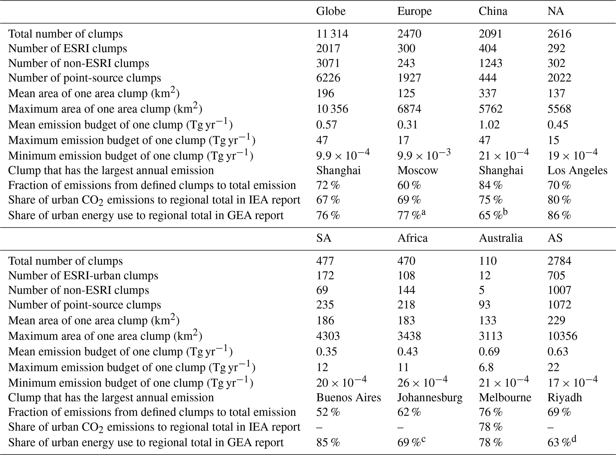
a Arithmetic mean of values for western Europe and eastern Europe. b In GEA report, this value corresponds to China and central Asia Pacific. c Arithmetic mean of values for Sub-Saharan Africa, northern Africa, and the Middle East. d Arithmetic mean of values for Pacific Asia and southern Asia.
Table 1 summarizes the clumps calculated for the globe, Europe (European Russia included), China, North America, South America, Africa, Australia, and Asia (China excluded). In total, our algorithm calculates 11 314 clumps, including 6226 point sources, 2017 ESRI clumps, and 3071 non-ESRI clumps. The clump with the largest annual emission budget is Shanghai, which emits 47 Mt C yr−1. A large fraction of the non-ESRI clumps is found within China mainly located near the southeastern coast, which may be explained by the recent rapid urbanization (Shan et al., 2018; Wang et al., 2016) in this region. This is not documented by the ESRI map. The large number of non-ESRI clumps in China highlights the necessity of considering emitters outside the major cities (at least) in this country. In addition, the mean area of an emission clump is larger in China than over other continents and regions. This is because the southeastern coast of China is densely populated, even within rural areas (yellow-green outside the urban area of the ESRI urban map in Fig. 4e), and because the emission rates per capita is also high in China compared to the world average (Janssens-Maenhout et al., 2017). As a result, our algorithm finds more non-ESRI clumps and larger areas for each clump in China than other regions.
Figure 5 shows the locations and annual emissions of the clumps. The densities of emission clumps are high in Europe, the eastern coast of the US, the eastern coast of China and India. Figure 6 shows the fractions of total emissions allocated to different clump categories. Globally, 27 % of the clumps are calculated as non-ESRI, but the total emission from these clumps is less than 13 % of the total emissions. Point sources form 55 % of the total number of clumps and 44 % of the total emissions. In China, however, point sources contribute only 21 % of the total number of clumps and 39 % of the total emissions, which may be explained by the fact that the power plants in China considered in CARMA dataset (and thus in ODIAC) are limited to the few larger power plants. Figure 7 shows the cumulative distribution of the number of clumps and their emissions for a few regions. Among ESRI clumps, 66 % of them have an annual emission below 1 Tg C yr−1, but the cumulative emission from these low emitting clumps only accounts for 22 % of the total emission from all ESRI clumps. The inflexion point in Fig. 7 (when the cumulative distribution curve turns from nearly 0 % to a fast increase) indicates the importance of clumps with annual emissions above this value. For non-ESRI clumps and point sources, the inflexion points are near 0.1 Tg C yr−1.

Figure 5The spatial distribution of emission-weighted centers of the emission clumps all over the globe. The inserted plots zoom into four regions that contain most of the clumps.

Figure 6The fraction of the number (bars) and the fraction of emissions (hatched bars) found in the three types of clumps for the European continent (European Russia included), China, North America (NA), South America (SA), Africa, Australia, Asia with China excluded (AS), and over the globe. The three colors represent ESRI clumps (yellow), non-ESRI clumps (green), and point-source clumps (red). The white-hatched bars indicate the fraction of ODIAC emissions that are not allocated to any clump by the algorithm.
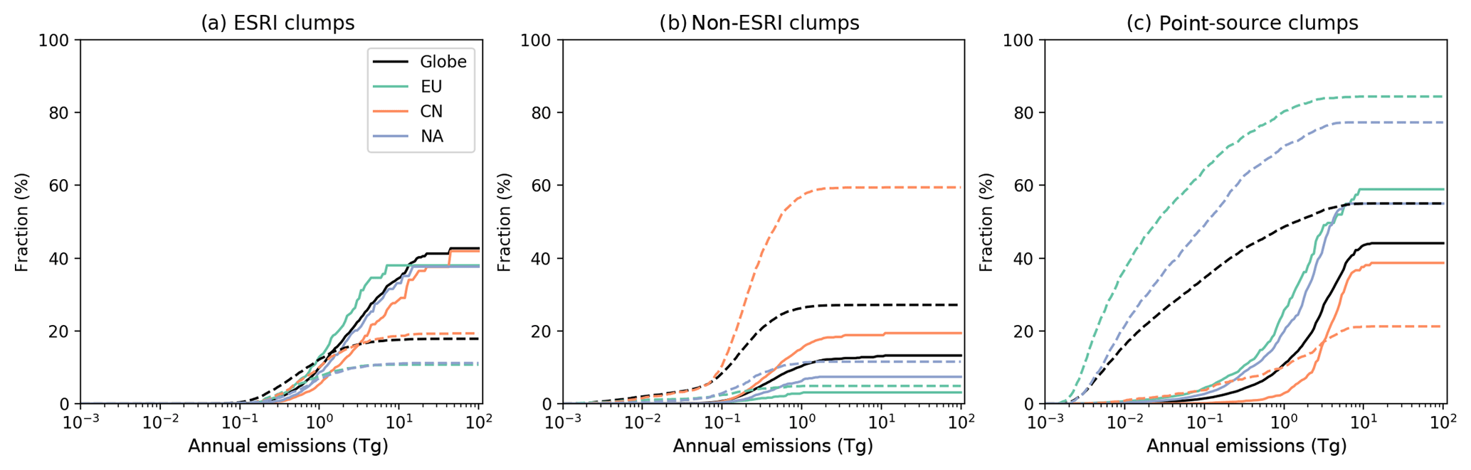
Figure 7Cumulative distributions of the number (dashed lines) of emission clumps and of the emissions (solid lines) of the clumps for three categories of clumps (see text).
3.2 Emission clumps based on other emission maps
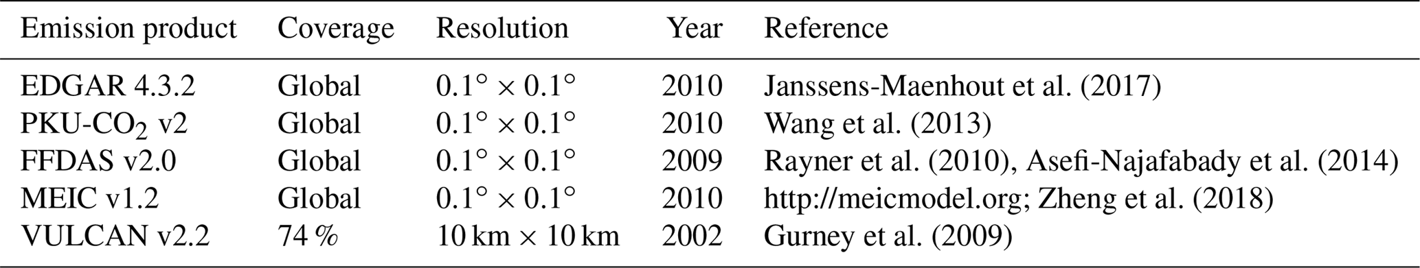
The clump results obviously depend on the input emission field. The ODIAC map is chosen as a reference because it is the only global map with a spatial resolution of ∼1 km that we are aware of. But there are other emission products with coarser resolution or only regional coverage. To test the dependency of calculated clumps on the choice of the emission map, we apply the algorithm to three alternative global emission maps and two regional emission maps (Table 2). The three global emission maps are PKU-CO2 v2 (Wang et al., 2013), FFDAS v2.0 (Rayner et al., 2010; Asefi-Najafabady et al., 2014), and EDGAR 4.3.2 (Janssens-Maenhout et al., 2017). The two regional emission maps are the Multi-resolution Emission Inventory (MEIC) v1.2 for China (http://meicmodel.org/, last access: 14 July 2018; Zheng et al., 2018) and the VULCAN inventory (Gurney et al., 2009) v2.2 for the contiguous US The resolutions of these emission maps are 0.1∘ or 10 km (Table 2), that is, about 12 times coarser than ODIAC. Note that some small (in terms of area) groups of grid cells with high emission rates at a finer resolution than 0.1∘ are averaged to the coarser grid cells in these coarser-resolution maps. The clumps derived from these alternative emission maps thus have a tendency to miss small clumps, compared to ODIAC. However, the comparison of the results for the largest clumps is still indicative of the robustness of the clump definition. The years of the additional emission maps are different from the year of ODIAC (Table 2) because some institutions have not released emission maps for 2016. We scale the different emission maps to the same national totals as ODIAC and we assume that the spatial distribution of clumps do not change significantly on the continental and global scales so that the differences in the year for different emission maps is not expected to have strong impacts on the clump results. We compare the fractions of emissions in alternative maps (X) covered by the clumps calculated from these map (X clumps) with the fraction covered by ODIAC clumps to see whether the ODIAC-clump results miss significant emissions from X. Because the resolution of ODIAC and alternative emission maps are different, when computing the X emissions covered by ODIAC clumps, we downscale map X to 30′′, assuming that emissions are distributed uniformly within each 0.1∘ or 10 km grid cell. Since the actual distribution of emissions within each 0.1∘ or 10 km grid cell is probably not uniform, this computation tends to overestimate the differences between ODIAC clumps and X clumps.
Table 2The alternative emission maps used to compare the results of ODIAC.
Each 30′′ grid cell is classified into a confusion matrix (CM) with four categories: (1) grid cell belongs to the ODIAC clump and X clump (true positive, TP), (2) grid cell belongs to the ODIAC clump but not to the X clump (false positive, FP), (3) grid cell belongs to the X clump but not to the ODIAC clump (false negative, FN), and (4) grid cell belongs neither in the ODIAC clump nor in the X clump (true negative, TN). The fractions of emissions in each CM category are computed for different regions. This comparison mainly allows us to verify whether the clumps delineated by the two thresholds are consistent using ODIAC and other maps.
We also checked the consistency of ESRI clumps between ODIAC clumps and X clumps with a similar CM. Each grid cell is classified into four categories: (1) grid cell belongs to the same ESRI clump in ODIAC and X (ESRI-TP), (2) grid cell belongs to ESRI clumps in both ODIAC and X but does not belong to the same ESRI clump (ESRI-DIFF), (3) grid cell only belongs to an ESRI clump either in ODIAC or X (ESRI-FALSE), and (4) grid cell does not belong to any ESRI clump in ODIAC or in X (ESRI-TN). Consistency for non-ESRI clumps is not really expected because X clumps tend to miss small clumps because of the underlying coarser-resolution maps. Consistency is not calculated for point-source clumps because not all emission products explicitly provide names for each power plant, making it difficult to determine whether the power plants from different maps within the same grid cell have the same infrastructure.
VULCAN is arguably the best emission map for the US, given its use of a large amount of relatively accurate data from local to national scales. PKU-CO2-v2 and MEIC v1.2, derived by Chinese institutions, used the exact locations of power plants and factories in China and detailed information of fuel consumption of each power plants and factories to estimate the point sources. They also used provincial data to distribute the nonpoint source emissions, resulting in more accurate estimates in the distribution of Chinese emissions than other global maps (Wang et al., 2013). EDGAR v4.3.2, developed by the Joint Research Center under the European Commission's service, has more accurate emission estimates in Europe. Therefore, we focus the clump consistency analysis between ODIAC and EDGAR v4.3.2 for Europe, between ODIAC, PKU-CO2 v2 and MEIC v1.2 for China, and between ODIAC and VULCAN v2.2 for the US.

Figure 8The fractions of emissions from corresponding emission products covered (1) by both ODIAC clumps and X clumps (red), (2) only by X clumps but not by ODIAC clumps (green), (3) by ODIAC clumps but not by X clumps (blue), and (4) by neither ODIAC clumps nor X clumps (pink). The thick black lines indicate the fractions of emissions in ODIAC covered by ODIAC clumps.
Figure 8 shows the results of the CM analysis. In general, there is a considerable fraction of national and regional emissions covered by both ODIAC clump and X clump (red bars). The sum of the fractions of TP (red bars) and TN (pink bars) are larger than 70 % for all countries and regions, indicating that the algorithm applied to different maps consistently allocates the same groups of emitting grid cells into clumps. In Europe, the fraction of EDGAR emissions allocated to EDGAR clumps (red plus blue bars in Fig. 8) is close to the fraction of ODIAC emissions allocated to ODIAC clumps (black line). In China, the fraction from MEIC is also close to that derived from ODIAC. But this fraction in PKU-CO2-v2 (54 %) is lower than that derived from ODIAC in China (84 %). The differences between these fractions derived from ODIAC, MEIC, and PKU-CO2-v2 indicate large uncertainties in the distribution of emissions in China. This fraction in VULCAN (46 %) is lower than that derived from ODIAC in the US (73 %). In addition, in all regions, the fractions of emissions allocated to X clumps (red plus blue bars) in X emission maps are all lower than those derived from ODIAC, indicating the emissions in ODIAC are more centralized toward populated areas than in other maps. This is attributed to the lack of line sources in ODIAC (Oda et al., 2018). The blue bars in Fig. 7, representing emissions from X maps that are not covered by ODIAC clumps, are less than 10 % of the total emissions in most cases, indicating that ODIAC clumps miss only a small fractions of emission hotspots compared to other plausible fossil fuel CO2 emission fields, even without any adjustment. However, ODIAC clumps would capture some low-emitting grid cells in other emission maps, as shown by the green bars in Fig. 8. Further investigation into the three types of clumps: ESRI clumps, non-ESRI clumps and point-sources clumps shows that the largest differences between ODIAC and X lie in the latter two types (Figs. S1–S3 in the Supplement). The non-ESRI clumps account for a small fraction of the total emissions (less than 20 % in general, Figs. 6 and S2), and the coherence in terms of fractions of emissions covered by non-ESRI clumps between different emission maps is less than 5 % (red bars in Fig. S2). There are also large disagreements in the emissions from point-source clumps between different emission maps, as displayed by Fig. S3.
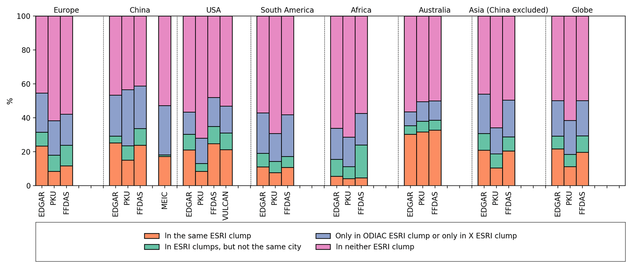
Figure 9The fractions of emissions from corresponding emission products covered (1) by the same ESRI clump from ODIAC and X (red), (2) by ESRI clumps in both ODIAC and X but do not belong to the same ESRI urban area (green), (3) only by one of the ESRI clump in either ODIAC or X (blue), and (4) by no ESRI clump in ODIAC or in X (pink).
Figure 9 examines the consistency of the fractions of emissions covered by the same clumps between ODIAC and any emission map X. The consistency indicated by the red and pink bars is larger than 70 %. The green bars are less than 10 % in general, indicating that there are not many emission grid cells connecting different large cities. The major differences between ESRI clumps derived from various emission maps come from grid cells near the borders of ESRI clumps so that they are classified as ESRI clumps or other clumps in different emission maps (blue bars).
4.1 Impacts of the sounding precision on the identification of emission clumps
In this study, we use the map of the urban area from ESRI and two thresholds to derive emission clumps. Threshold-1 determines the cores of the clumps, corresponding to a XCO2 enhancement larger than the precision (0.5 ppm) of individual soundings without atmospheric horizontal transport (see Sect. 2.2 and Appendix). The precision largely depends on the designs and configurations of different satellites. In this section, we test the sensitivity of the clumps to different assumptions on threshold-1 related to the precision of an individual sounding. The results listed in Table 3 show that the number of clumps are very sensitive to threshold-1 or individual XCO2 sounding precision. However, the fractions of emissions covered by the clumps do not change significantly with threshold-1. The total number of clumps is reduced by 34 % when the precision of an individual XCO2 measurement is degraded to 1.0 ppm, compared to that obtained assuming 0.5 ppm, but the fraction of emissions covered by all clumps is only reduced from 72 % to 61 %, e.g., 15 % relative change. This indicates that a larger value of threshold-1 mainly removes clumps with small emissions. On the other hand, the number and fraction of emissions covered by point-source clumps are not sensitive to threshold-1 due to the fact that their emissions are highly concentrated in limited area. On the contrary, the number and emissions associated with non-ESRI clumps are the most sensitive to the precision.
Table 3The sensitivity of the number of emission clumps (integers before parentheses) and the fractions of emissions covered by the emission clumps (values in the parentheses) to the global total of the thresholds in the clump algorithm.
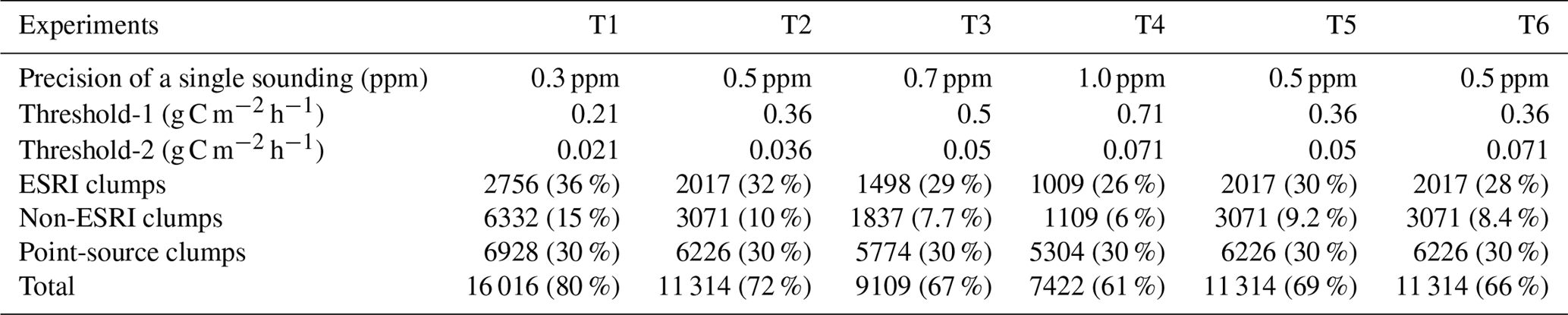
Threshold-2 is used to define which grid cells shall be aggregated with the cores to form a clump. In this study, threshold-2 is chosen an order of magnitude smaller than threshold-1. This choice is somewhat arbitrary to include some marginal areas. Such marginal area accounts for the fact that the outskirts of the cities could also contribute to the city cores. In addition, the marginal area ensures that the effective clumps (e.g., the cores of the clumps) will always be accounted for in the clump map within a short time span (typically within one year to among few years). With this default choice of threshold-2, the fraction of emissions from clumps to the total emissions is occasionally close to the estimate of the share of CO2 emissions or energy use from cities to regional total in EIA and GEA (Table 1). The last two columns in Table 3 list the results for different values of threshold-2. Threshold-2 mainly impacts the extent of surrounding grid cells near the cores of each area clump. When threshold-2 is chosen to be 0.071 g C m−2 h−1 (twice as large as the default one), keeping threshold-1 as 0.36 g C m−2 h−1, the fraction of emissions covered by the clumps to the global total is reduced from 72 % (default result, T2) to 66 %. The comparison between the results of T2, T6, and T4 in Table 3 shows that the identification of non-ESRI clumps is more sensitive to threshold-1 (precision), while the identification of ESRI clumps is more sensitive to threshold-2 (grid cells around cores in ESRI urban areas).
4.2 Impact of using ODIAC on the identification of emission clumps
ODIAC used a nighttime light as a proxy for the spatial distribution of emissions. The accuracy of the proxy in representing the distribution of actual emissions largely impacts the extent of the clumps. For example, compared with other emission products, ODIAC does not capture line source emissions such as on-road transportation (Oda et al., 2018; Gurney et al., 2019). The satellite observations of CO indicated significant CO enhancement over major roads (Borsdorff et al., 2019). Since our clump map is derived from the ODIAC emission product, some of the roads that generate significant XCO2 plumes may be missed by the clumps defined in this study. As the ODIAC team is planning to include transportation network data in their emission product (Oda et al., 2018), our clump map could be updated with a new version of ODIAC.
Figure 8 shows that if the ODIAC clumps are applied to other emission maps even without any adjustment, a majority of emission hotspots (indicated by red plus green bars in Fig. 8) are still included in the clump areas. However, Fig. 9 shows that there are large differences in the way emitting grid cells are grouped depending on the input emission map. When multiplying the map of ODIAC clumps by another X emission map, the difference between the emissions from ODIAC and the emissions from the same area in the X map, for a single clump, ranges between 0 % and 165 % (5th–95th percentiles). The relative differences tend to be larger for small clumps than large ones. For the monitoring of fossil fuel CO2 emissions from space, these results highlight the necessity of objectively associating the observed CO2 plumes with underlying emitting regions.
In this study, the clumps are only defined based on the ODIAC emission map for the year 2016. However, in the regions experiencing fast urbanization rates, the spatial distribution of emissions are also changing rapidly. In order to build an operational observing system in the near future, it is also necessary to consistently update the clump definition based on the latest emission maps to track the trends in the emissions and CO2 plumes for growing cities.
4.3 Implications for future inversion studies
The emission clump is a valuable concept relevant for the monitoring of fossil fuel CO2 emissions from satellites. The emission clumps defined in this study have at least one grid cell that will generate an excess of XCO2 of at least 0.5 ppm over a morning period of 6 h, assuming no atmospheric horizontal transport. This assumption is optimistic in terms of detectability of XCO2 plumes. In reality, when accounting for wind advection or vegetation fluxes near a clump, XCO2 enhancement in plumes may be smaller than 0.5 ppm and therefore harder to detect with imagers. In this sense, the emissions covered in emission clumps derived from such an assumption conservatively define the upper fraction of fossil fuel CO2 emissions that could be constrained by XCO2 imagery. In addition, the sampling of plumes will be reduced in presence of clouds and will suffer from XCO2 biases related to aerosol loads (Broquet et al., 2018; Pillai et al., 2016). The emission clumps defined in this study provide a test bed for assessing the potential of satellite imagery for monitoring fossil fuel CO2 emissions. In the future, global and regional inversion systems and observing system simulation experiment (OSSE) frameworks shall be developed using emission fields classified into clumps. Such inversions and OSSE studies will play a critical role in the deployment of new observation strategies and assessing the potential of these observing systems for assessing the fossil fuel CO2 emissions (e.g., Broquet et al., 2018; Turner et al., 2016; Pillai et al., 2016).
The ODIAC2017 data product can be downloaded from the website http://db.cger.nies.go.jp/dataset/ODIAC/ (last access: 1 November 2017; or https://doi.org/10.17595/20170411.001; Oda and Maksyutov, 2015). The TIMES data product can be downloaded from http://cdiac.ess-dive.lbl.gov/ftp/Nassar_Emissions_Scale_Factors/ (last access: 1 November 2017). The clump map can be downloaded from https://doi.org/10.6084/m9.figshare.7217726.v1 (Wang et al., 2018).
In this study, we have identified a set of emission clumps with large emission rates (in g C m−2 h−1) from a high-resolution emission inventory. These clumps will generate individual atmospheric XCO2 plumes that may be observed from space. This method identifies the clump cores using an ESRI map of major urban area and a high threshold related to the precision of XCO2 measurements from planned satellites. It uses a low threshold and an RW algorithm to consider the area in the vicinity of the cores and split the area between different clumps based on the spatial gradients in the emission field. The emission clumps defined in this study depict the emitting hotspots around the globe that are relevant for the monitoring of fossil fuel CO2 emissions from the satellites measurements. The clumps are derived with a transboundary approach, bypassing any artificial border imposed by national emissions. In total, the emission clumps cover 72 % of the total emissions in the original ODIAC. They defines the scales and regions of monitoring the short-term temporal profiles and long-term trends in fossil fuel CO2 emissions, which might be very useful for the global stocktaking exercise by the UNFCCC. The clumps that have been identified here span a large range of emission. Given actual atmospheric transport condition, it is not clear whether those in the low range of emission generate an atmospheric CO2 plume that can be identified from space. The presence of cloud cover may also challenge the detection of XCO2 plumes and thus the estimate of emissions using space-borne measurements. Which fraction of the identified clump can be observed from space and what accuracy can be expected from the atmospheric inversion requires an OSSE framework, which shall be developed in a future paper.
We make a calculation of the emission flux that would generate a 0.5 ppm excess of XCO2 during 6 h without wind. This is a conservative case with the accumulation of all emissions in the air column. The 0.5 ppm XCO2 is taken as the individual sounding precision of a satellite CO2 imager. Assuming a constant emission rate F (g C m−2 h−1) during 6 h, the XCO2 excess (XCO2, ppm) is given by the following:
where MC ( kg mol−1) represented the molar mass of C, Xair (mol m−2) represented the molar quantity of air mass in the air column. The Xair could be approximated by the following:
where Psurf ( Pa) represents the surface pressure, g (=9.8 m s−2) represents the acceleration of gravity, Mair ( kg mol−1) represents the average molar mass of air. Thus, the minimum emissions F∗ that would generate a 0.5 ppm excess of XCO2 is computed g m−2 h−1.
The supplement related to this article is available online at: https://doi.org/10.5194/essd-11-687-2019-supplement.
PC designed the research, YW performed the research and developed the algorithm. GB, FMB, FL, DS and YS contributed to the development of the algorithm. YM and AL provided information about the LEO imager on Sentinel missions and supervised the research. TO provided the ODIAC emission map. GJM provided the EDGAR emission map. BZ provided the MEIC emission map. HX and ST provided the PKU-CO2 emission map. KRG and GR provided VULCAN, the emission map. All authors discussed the results and contributed to the final manuscript.
The authors declare that they have no conflict of interest.
The views expressed here can in no way be taken to reflect the official opinion of ESA.
This research was carried out at the Laboratoire des Sciences du Climat et de l'Environnement, CEA-CNRS-UVSQ-Université Paris Saclay, 91191, Gif-sur-Yvette, France, under a contract with the European Space Agency (ESA). We thank the two reviewers and the editor whose comments and suggestions helped improve and clarify this manuscript.
This research has been supported by the European Space Agency (ESA) (grant no. 4000120184/17/NL/FF/mg).
This paper was edited by Thomas Blunier and reviewed by Peter Rayner and Rong Wang.
Asefi-Najafabady, S., Rayner, P. J., Gurney, K. R., McRobert, A., Song, Y., Coltin, K., Huang, J., Elvidge, C., and Baugh, K.: A multiyear, global gridded fossil fuel CO2emission data product: Evaluation and analysis of results, J. Geophys. Res., 119, 10213–10231, https://doi.org/10.1002/2013jd021296, 2014.
Boden, T. A., Marland, G., and Andres, R. J.: Global, Regional, and National Fossil-Fuel CO2 Emissions, available at: http://cdiac.ess-dive.lbl.gov/epubs/ndp/ndp058/ndp058_v2016.html (last access: 2 August 2018), 2016.
Borsdorff, T., aan de Brugh, J., Pandey, S., Hasekamp, O., Aben, I., Houweling, S., and Landgraf, J.: Carbon monoxide air pollution on sub-city scales and along arterial roads detected by the Tropospheric Monitoring Instrument, Atmos. Chem. Phys., 19, 3579–3588, https://doi.org/10.5194/acp-19-3579-2019, 2019.
Bovensmann, H., Buchwitz, M., Burrows, J. P., Reuter, M., Krings, T., Gerilowski, K., Schneising, O., Heymann, J., Tretner, A., and Erzinger, J.: A remote sensing technique for global monitoring of power plant CO2 emissions from space and related applications, Atmos. Meas. Tech., 3, 781–811, https://doi.org/10.5194/amt-3-781-2010, 2010.
Bréon, F. M., Broquet, G., Puygrenier, V., Chevallier, F., Xueref-Remy, I., Ramonet, M., Dieudonné, E., Lopez, M., Schmidt, M., Perrussel, O., and Ciais, P.: An attempt at estimating Paris area CO2 emissions from atmospheric concentration measurements, Atmos. Chem. Phys., 15, 1707–1724, https://doi.org/10.5194/acp-15-1707-2015, 2015.
Broquet, G., Bréon, F.-M., Renault, E., Buchwitz, M., Reuter, M., Bovensmann, H., Chevallier, F., Wu, L., and Ciais, P.: The potential of satellite spectro-imagery for monitoring CO2 emissions from large cities, Atmos. Meas. Tech., 11, 681–708, https://doi.org/10.5194/amt-11-681-2018, 2018.
Buchwitz, M., Reuter, M., Bovensmann, H., Pillai, D., Heymann, J., Schneising, O., Rozanov, V., Krings, T., Burrows, J. P., Boesch, H., Gerbig, C., Meijer, Y., and Löscher, A.: Carbon Monitoring Satellite (CarbonSat): assessment of atmospheric CO2 and CH4 retrieval errors by error parameterization, Atmos. Meas. Tech., 6, 3477–3500, https://doi.org/10.5194/amt-6-3477-2013, 2013.
Cao, X., Chen, J., Imura, H., and Higashi, O.: A SVM-based method to extract urban areas from DMSP-OLS and SPOT VGT data, Remote Sens. Environ., 113, 2205–2209, https://doi.org/10.1016/j.rse.2009.06.001, 2009.
Chatterjee, A., Gierach, M. M., Sutton, A. J., Feely, R. A., Crisp, D., Eldering, A., Gunson, M. R., O'Dell, C. W., Stephens, B. B., and Schimel, D. S.: Influence of El Niño on atmospheric CO2 over the tropical Pacific Ocean: Findings from NASA's OCO-2 mission, Science, 358, eaam5776, https://doi.org/10.1126/science.aam5776, 2017.
Ciais, P., Crisp, D., Denier van der Gon, H. A. C., Engelen, R., Heimann, M., Janssens-Maenhout, G., Rayner, P., and Scholze, M.: Towards a European Operational Observing System to Monitor Fossil CO2 emissions, European Commission Directorate-General for Internal Market, Industry, Entrepreneurship and SMEs Directorate I – Space Policy, Copernicus and Defence, Brussels, Belgium, 2015.
Creutzig, F., Baiocchi, G., Bierkandt, R., Pichler, P.-P., and Seto, K. C.: Global typology of urban energy use and potentials for an urbanization mitigation wedge, P. Natl. Acad. Sci., 112, 6283–6288, https://doi.org/10.1073/pnas.1315545112, 2015.
Doll, C. N. H. and Pachauri, S.: Estimating rural populations without access to electricity in developing countries through night-time light satellite imagery, Energ. Policy, 38, 5661–5670, https://doi.org/10.1016/j.enpol.2010.05.014, 2010.
Eldering, A., Wennberg, P. O., Crisp, D., Schimel, D. S., Gunson, M. R., Chatterjee, A., Liu, J., Schwandner, F. M., Sun, Y., O'Dell, C. W., Frankenberg, C., Taylor, T., Fisher, B., Osterman, G. B., Wunch, D., Hakkarainen, J., Tamminen, J., and Weir, B.: The Orbiting Carbon Observatory-2 early science investigations of regional carbon dioxide fluxes, Science, 358, eaam5745, https://doi.org/10.1126/science.aam5745, 2017.
Elvidge, C. D., Baugh, K. E., Kihn, E. A., Kroehl, H. W., and Davis, E. R.: Mapping city lights with nighttime data from the DMSP Operational Linescan System, Photogramm. Eng. Rem. S., 63, 727–734, 1997.
Grady, L.: Random Walks for Image Segmentation, IEEE T. Pattern Anal., 28, 1768–1783, https://doi.org/10.1109/TPAMI.2006.233, 2006.
Gurney, K. R., Mendoza, D. L., Zhou, Y., Fischer, M. L., Miller, C. C., Geethakumar, S., and Can, S. de la R.: High Resolution Fossil Fuel Combustion CO2 Emission Fluxes for the United States, Environ. Sci. Technol., 43, 5535–5541, 2009.
Gurney, K. R., Liang, J., O'Keeffe, D., Patarasuk, R., Hutchins, M., Huang, J., Rao, P., and Song, Y.: Comparison of Global Downscaled Versus Bottom-Up Fossil Fuel CO2 Emissions at the Urban Scale in Four U.S. Urban Areas, J. Geophys. Res.-Atmos., 124, 2823–2840, https://doi.org/10.1029/2018JD028859, 2019.
Hakkarainen, J., Ialongo, I., and Tamminen, J.: Direct space-based observations of anthropogenic CO2 emission areas from OCO-2, Geophys. Res. Lett., 43, 2016GL070885, https://doi.org/10.1002/2016GL070885, 2016.
Huang, X., Schneider, A., and Friedl, M. A.: Mapping sub-pixel urban expansion in China using MODIS and DMSP/OLS nighttime lights, Remote Sens. Environ., 175, 92–108, https://doi.org/10.1016/j.rse.2015.12.042, 2016.
International Energy Agency (IEA): World Energy Outlook 2008, OECD Publishing, Paris, France, 2008.
Janssens-Maenhout, G., Crippa, M., Guizzardi, D., Muntean, M., Schaaf, E., Dentener, F., Bergamaschi, P., Pagliari, V., Olivier, J. G. J., Peters, J. A. H. W., van Aardenne, J. A., Monni, S., Doering, U., and Petrescu, A. M. R.: EDGAR v4.3.2 Global Atlas of the three major Greenhouse Gas Emissions for the period 1970–2012, Earth Syst. Sci. Data Discuss., https://doi.org/10.5194/essd-2017-79, 2017.
Lauvaux, T., Miles, N. L., Deng, A., Richardson, S. J., Cambaliza, M. O., Davis, K. J., Gaudet, B., Gurney, K. R., Huang, J., O'Keefe, D., Song, Y., Karion, A., Oda, T., Patarasuk, R., Razlivanov, I., Sarmiento, D., Shepson, P., Sweeney, C., Turnbull, J., and Wu, K.: High-resolution atmospheric inversion of urban CO2 emissions during the dormant season of the Indianapolis Flux Experiment (INFLUX), J. Geophys. Res., 121, 2015JD024473, https://doi.org/10.1002/2015JD024473, 2016.
Letu, H., Hara, M., Yagi, H., Naoki, K., Tana, G., Nishio, F., and Shuhei, O.: Estimating energy consumption from night-time DMPS/OLS imagery after correcting for saturation effects, Int. J. Remote Sens., 31, 4443–4458, https://doi.org/10.1080/01431160903277464, 2010.
Li, X. and Zhou, Y.: Urban mapping using DMSP/OLS stable night-time light: a review, Int. J. Remote Sens., 38, 6030–6046, https://doi.org/10.1080/01431161.2016.1274451, 2017.
Li, X., Wang, X., Zhang, J., and Wu, L.: Allometric scaling, size distribution and pattern formation of natural cities, Palgrave Communications, 1, palcomms201517, https://doi.org/10.1057/palcomms.2015.17, 2015.
Liu, L. and Leung, Y.: A study of urban expansion of prefectural-level cities in South China using night-time light images, Int. J. Remote Sens., 36, 5557–5575, https://doi.org/10.1080/01431161.2015.1101650, 2015.
Liu, X., Hu, G., Ai, B., Li, X., and Shi, Q.: A Normalized Urban Areas Composite Index (NUACI) Based on Combination of DMSP-OLS and MODIS for Mapping Impervious Surface Area, Remote Sens., 7, 17168–17189, https://doi.org/10.3390/rs71215863, 2015.
Nassar, R., Napier-Linton, L., Gurney, K. R., Andres, R. J., Oda, T., Vogel, F. R., and Deng, F.: Improving the temporal and spatial distribution of CO2emissions from global fossil fuel emission data sets, J. Geophys. Res., 118, 917–933, https://doi.org/10.1029/2012jd018196, 2013.
Nassar, R., Hill, T. G., McLinden, C. A., Wunch, D., Jones, D. B. A., and Crisp, D.: Quantifying CO2 Emissions From Individual Power Plants From Space, Geophys. Res. Lett., 44, 10045–10053, https://doi.org/10.1002/2017GL074702, 2017.
O'Brien, D. M., Polonsky, I. N., Utembe, S. R., and Rayner, P. J.: Potential of a geostationary geoCARB mission to estimate surface emissions of CO2, CH4 and CO in a polluted urban environment: case study Shanghai, Atmos. Meas. Tech., 9, 4633–4654, https://doi.org/10.5194/amt-9-4633-2016, 2016.
Oda, T. and Maksyutov, S.: A very high-resolution (1 km × 1 km) global fossil fuel CO2 emission inventory derived using a point source database and satellite observations of nighttime lights, Atmos. Chem. Phys., 11, 543–556, https://doi.org/10.5194/acp-11-543-2011, 2011.
Oda, T. and Maksyutov, S.: ODIAC Fossil Fuel CO2 Emissions Dataset, Center for Global Environmental Research, National Institute for Environmental Studies, https://doi.org/10.17595/20170411.001, 2015.
Oda, T., Maksyutov, S., and Andres, R. J.: The Open-source Data Inventory for Anthropogenic CO2, version 2016 (ODIAC2016): a global monthly fossil fuel CO2 gridded emissions data product for tracer transport simulations and surface flux inversions, Earth Syst. Sci. Data, 10, 87–107, https://doi.org/10.5194/essd-10-87-2018, 2018.
Pillai, D., Buchwitz, M., Gerbig, C., Koch, T., Reuter, M., Bovensmann, H., Marshall, J., and Burrows, J. P.: Tracking city CO2 emissions from space using a high-resolution inverse modelling approach: a case study for Berlin, Germany, Atmos. Chem. Phys., 16, 9591–9610, https://doi.org/10.5194/acp-16-9591-2016, 2016.
Polonsky, I. N., O'Brien, D. M., Kumer, J. B., O'Dell, C. W., and the geoCARB Team: Performance of a geostationary mission, geoCARB, to measure CO2, CH4 and CO column-averaged concentrations, Atmos. Meas. Tech., 7, 959–981, https://doi.org/10.5194/amt-7-959-2014, 2014.
Rayner, P. J., Raupach, M. R., Paget, M., Peylin, P., and Koffi, E.: A new global gridded data set of CO2 emissions from fossil fuel combustion: Methodology and evaluation, J. Geophys. Res., 115, D19306, https://doi.org/10.1029/2009jd013439, 2010.
Seto, K. C., Dhakal, S., Bigio, A., Blanco, H., Delgado, G. C., Dewar, D., Huang, L., Inaba, A., Kansal, A., and Lwasa, S.: Human settlements, infrastructure and spatial planning, in: Climate Change 2014: Mitigation of Climate Change: Contribution of Working Group III to the Fifth Assessment Report of the Intergovernmental Panel on Climate Change, chap. 12, 923–1000, IPCC, Geneva, Switzerland, 2014.
Shan, Y., Guan, D., Hubacek, K., Zheng, B., Davis, S. J., Jia, L., Liu, J., Liu, Z., Fromer, N., Mi, Z., Meng, J., Deng, X., Li, Y., Lin, J., Schroeder, H., Weisz, H., and Schellnhuber, H. J.: City-level climate change mitigation in China, Sci. Adv., 4, eaaq0390, https://doi.org/10.1126/sciadv.aaq0390, 2018.
Staufer, J., Broquet, G., Bréon, F.-M., Puygrenier, V., Chevallier, F., Xueref-Rémy, I., Dieudonné, E., Lopez, M., Schmidt, M., Ramonet, M., Perrussel, O., Lac, C., Wu, L., and Ciais, P.: The first 1-year-long estimate of the Paris region fossil fuel CO2 emissions based on atmospheric inversion, Atmos. Chem. Phys., 16, 14703–14726, https://doi.org/10.5194/acp-16-14703-2016, 2016.
Su, Y., Chen, X., Wang, C., Zhang, H., Liao, J., Ye, Y., and Wang, C.: A new method for extracting built-up urban areas using DMSP-OLS nighttime stable lights: a case study in the Pearl River Delta, southern China, GISci. Remote Sens., 52, 218–238, https://doi.org/10.1080/15481603.2015.1007778, 2015.
Turner, A. J., Shusterman, A. A., McDonald, B. C., Teige, V., Harley, R. A., and Cohen, R. C.: Network design for quantifying urban CO2 emissions: assessing trade-offs between precision and network density, Atmos. Chem. Phys., 16, 13465–13475, https://doi.org/10.5194/acp-16-13465-2016, 2016.
United Nations Framework Convention on Climate Change (UNFCCC): Adoption of the Paris agreement, Paris, France, 2015.
Wang, Q., Wu, S., Zeng, Y., and Wu, B.: Exploring the relationship between urbanization, energy consumption, and CO2 emissions in different provinces of China, J. Renew. Sustain. Ener., 54, 1563–1579, https://doi.org/10.1016/j.rser.2015.10.090, 2016.
Wang, R., Tao, S., Ciais, P., Shen, H. Z., Huang, Y., Chen, H., Shen, G. F., Wang, B., Li, W., Zhang, Y. Y., Lu, Y., Zhu, D., Chen, Y. C., Liu, X. P., Wang, W. T., Wang, X. L., Liu, W. X., Li, B. G., and Piao, S. L.: High-resolution mapping of combustion processes and implications for CO2 emissions, Atmos. Chem. Phys., 13, 5189–5203, https://doi.org/10.5194/acp-13-5189-2013, 2013.
Wang, Y., Ciais, P., Broquet, G., Bréon, F.-M., Oda, T., Lespinas, F., Meijer, Y., Loescher, A., Janssens-Maenhout, G., Zheng, B., Xu, H., Tao, S., Santaren, D., and Su, Y.: A global map of emission clumps for future monitoring of fossil fuel CO2 emissions from space, Figshare, https://doi.org/10.6084/m9.figshare.7217726.v1, 2018.
Zheng, B., Tong, D., Li, M., Liu, F., Hong, C., Geng, G., Li, H., Li, X., Peng, L., Qi, J., Yan, L., Zhang, Y., Zhao, H., Zheng, Y., He, K., and Zhang, Q.: Trends in China's anthropogenic emissions since 2010 as the consequence of clean air actions, Atmos. Chem. Phys., 18, 14095–14111, https://doi.org/10.5194/acp-18-14095-2018, 2018.
Zhou, Y., Smith, S. J., Elvidge, C. D., Zhao, K., Thomson, A., and Imhoff, M.: A cluster-based method to map urban area from DMSP/OLS nightlights, Remote Sens. Environ., 147, 173–185, 2014.
Zhou, Y., Smith, S. J., Zhao, K., Imhoff, M., Thomson, A., Bond-Lamberty, B., Asrar, G. R., Zhang, X., He, C., and Elvidge, C. D.: A global map of urban extent from nightlights, Environ. Res. Lett., 10, 054011, https://doi.org/10.1088/1748-9326/10/5/054011, 2015.