the Creative Commons Attribution 4.0 License.
the Creative Commons Attribution 4.0 License.
 | 30 Apr 2019
A high-resolution image time series of the Gorner Glacier – Swiss Alps – derived from repeated unmanned aerial vehicle surveys
Lionel Benoit
Aurelie Gourdon
Raphaël Vallat
Inigo Irarrazaval
Mathieu Gravey
Benjamin Lehmann
Günther Prasicek
Dominik Gräff
Frederic Herman
Gregoire Mariethoz
Modern drone technology provides an efficient means to monitor the response of alpine glaciers to climate warming. Here we present a new topographic dataset based on images collected during 10 UAV surveys of the Gorner Glacier glacial system (Switzerland) carried out approximately every 2 weeks throughout the summer of 2017. The final products, available at https://doi.org/10.5281/zenodo.2630456 (Benoit et al., 2018), consist of a series of 10 cm resolution orthoimages, digital elevation models of the glacier surface, and maps of ice surface displacement. Used on its own, this dataset allows mapping of the glacier and monitoring surface velocities over the summer at a very high spatial resolution. Coupled with a classification or feature detection algorithm, it enables the extraction of structures such as surface drainage networks, debris, or snow cover. The approach we present can be used in the future to gain insights into ice flow dynamics.
- Article
(4122 KB) - Full-text XML
- BibTeX
- EndNote


Glacier ice flows by deformation and sliding in response to gravitational forces. As a glacier moves, internal pressure gradients and stresses create visible surface features such as glacial ogives and crevasses (Cuffey and Paterson, 2010). Furthermore, the surface of glaciers is also shaped by local weather conditions, which are responsible for the snow accumulation and ablation. Related processes generate distinct morphologies such as supraglacial streams, ponds, and lakes.
Glacier surface features evolve continuously, and these changes provide insights into the structure, internal dynamics, and mass balance of the glacier. Important efforts have been made to monitor glacier surfaces, from early stakes measurements at the end of the 19th century (Chen and Funk, 1990) to present-day in situ topographic surveys (Ramirez et al., 2001; Aizen et al., 2006; Dunse et al., 2012; Benoit et al., 2015) and remotely sensed data acquired from diverse platforms: ground-based devices (Gabbud et al., 2015; Piermattei at al., 2015), aircraft (Baltsavias et al., 2001; Mertes et al., 2017), or satellites (Herman et al., 2011; Kääb et al., 2012; Dehecq et al., 2015; Berthier et al., 2014). Recently, the development of unmanned aerial vehicles (UAVs) has enabled glaciologists to carry out their own aerial surveys autonomously, rapidly, and at reasonable costs (Whitehead et al., 2013; Immerzeel et al., 2014; Bhardwaj et al., 2016; Jouvet et al., 2017; Rossini et al., 2018). This technology is particularly attractive to map alpine glaciers whose limited size allows a satisfying coverage at a centimeter to decimeter spatial resolution.
Here we provide a homogenized and high-resolution remote-sensing dataset covering about 10 km2 of the ablation zone of the Gorner Glacier glacial system (Valais, Switzerland, Fig. 1). The raw images have been acquired by UAV flights carried out approximately every 2 weeks during the summer of 2017 (from 29 May to 30 October). The dataset comprises 10 consecutive digital elevation models (DEMs) and associated orthomosaics of the area of interest at a 10 cm resolution. It is therefore one of the most exhaustive surveys of the short-term surface evolution of a temperate glacier currently available. Geometrical coherence of the dataset is ensured through the application of comprehensive photogrammetric processing (i.e., images are ortho-rectified and properly scaled). In addition, the orthomosaics are stackable thanks to a co-registration procedure. The dataset can therefore be seen as a high-resolution time lapse of the Gorner Glacier ablation zone, combining spectral (orthomosaics) and geometrical (DEMs) information on the glacier surface. In addition to orthomosaics and DEMs that are snapshots of the area of interest, we also provide a product that we call matching maps (MMs) to achieve temporal monitoring of the glacier. In practice, a MM associates with each pixel of an orthomosaic (respectively a DEM) the corresponding pixel in the next orthomosaic recorded 2 weeks later. MMs can then be used to track the flow of ice over time, and in turn to quantify ice surface displacements.
Potential uses of this dataset are numerous. Single orthomosaics and DEMs can be used to map the surface of the glacier and to extract features of interest such as the surface drainage network (Yang and Smith, 2012; Rippin et al., 2015), debris, or snow cover (Racoviteanu and Williams, 2012). Alternatively, the complete time series of orthomosaics and DEMs can be used for detection and quantification of changes at the surface of the glacier (Barrand et al., 2009; Berthier et al., 2016; Fugazza et al., 2018). Finally, the time lapse coupled with the MMs is an interesting tool to monitor ice surface velocity and deformation (Ryan et al., 2015; Kraaijenbrink et al., 2016), and in turn ice flow dynamics at the glacier surface (Brun et al., 2018). The MMs provide a quantification of the ice velocity at every location on the surface of the glacier, which can be used to calibrate or to validate ice flow models, especially for the Gorner Glacier, which was extensively used as a modeling benchmark (see for instance Werder and Funk, 2009; Riesen et al., 2010; Sugiyama et al., 2010; Werder et al., 2013).
2.1 Study site
The Gorner Glacier is located in the Valais Alps in southern Switzerland (Fig. 1a). It is part of a glacier system involving five tributaries and ranges from 2200 to 4634 m a.s.l. (Fig. 1b). The ablation area, which is the main focus of this study, is a 4 km long and relatively flat ice tongue (slope around 6 %, i.e., 3.4∘) that is deeply incised by meltwater channels and partially debris covered (Fig. 1c). This ablation area is preceded by a steeper part (southwest of the Monte Rosa Hut, Fig. 1c) characterized by the presence of numerous crevasses. The entire Gorner Glacier system (i.e., the terminal tongue and its five tributaries) covers an area of almost 50 km2 and its central flow line is 12 km long, making it one of the largest European glaciers (Sugiyama et al., 2010).
The Gorner Glacier system has been widely studied since the 1970s due to its significant size, its accessibility, and because a glacier-dammed lake threatened the downstream Matter valley with glacier outburst floods (Sugiyama et al., 2010; Werder et al., 2009, 2013). The long history of glaciological studies in this area has shown that the mass balance of the Gorner Glacier system was stable from the 1930s to the early 1980s, and significantly dropped since then (Huss et al., 2012). This can be associated with the rise of its equilibrium line altitude (ELA) due to an increase in the local average yearly temperature. The ELA is at around 3300 m today according to studies carried out at the neighboring Findel Glacier (Sold et al., 2016).
In this context, the current dataset aims at complementing existing studies about the Gorner Glacier system by documenting the behavior of its ablation zone during an entire summer, at a time when this glacial system is thought to be out of equilibrium with a clear trend toward glacial retreat. In particular, this dataset focuses on the monitoring of the glacier surface at high spatial and temporal resolution.
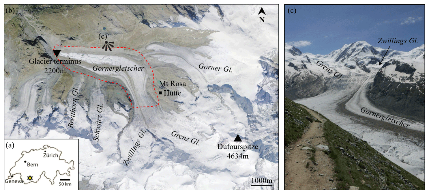
Figure 1The Gorner Glacier system. (a) Situation map. (b) Overview of the Gorner Glacier system; dashed red line: area of interest. (c) Picture of the glacier tongue.
2.2 UAV surveys
The primary data are RGB images acquired by repeated UAV surveys over an area of 10 km2. A fully autonomous fixed-wing UAV of type eBee from SenseFly, equipped with a 20-megapixel SenseFly S.O.D.A camera, has been used for image acquisition (Vallet et al., 2011). The camera was static within the UAV body (no gimbal) and therefore all pictures are quasi-nadir (i.e., images are taken with an angle ±10∘ from the vertical line). For flight planning and UAV piloting, the eMotion3 software was used.
Raw images were acquired with a ground resolution ranging from 7.3 to 8.8 cm for the glaciated parts of the area of interest. For the requirements of photogrammetric processing, flight plans have been designed to allow for an overlap between images ranging from 70 % to 85 % in the flight direction and from 60 % to 70 % in the cross-flight direction. These specifications have led to flight altitudes ranging from 300 to 600 m above ground. The flight time was limited to about 30 min in field conditions. Thus, the coverage of the full area of interest required four to eight separate flights per session, i.e., each day of acquisition (Table 1). Overall, 10 sessions were conducted in 2017, from 29 May to 30 October. The main features of these flights are summarized in Table 1.
Table 1UAV flights carried out for raw glacier image acquisition.

3.1 Generation of co-registered orthomosaics and DEMs
Pictures have been processed separately for each acquisition date with the photogrammetric software pix4DMapper version 3.1 (Vallet et al., 2011, Fig. 2) using default parameters for nadir flights (see the processing reports for details about these parameters). The output resolution has been set to 10 cm per pixel in order to prescribe a constant resolution across all final products. During the photogrammetric processing, the raw pictures are first oriented by bundle adjustment, and then a DEM and an ortho-rectified image (orthomosaic) are generated for each day of interest. Since the only geolocation information included into the bundle adjustment procedure is the trajectory of the UAV derived from code-only GPS data, the initial geo-referencing of the orthomosaics and DEMs is limited to a few meters. To improve the coherence of the co-referencing of the different sessions, all products are co-registered to the reference of the 9 June acquisition (Fig. 2). To this end, the coordinates of several stable points of the landscape (16 to 70 among a set of 74; see Table 2 and Fig. 4) are extracted from the bundle adjustment of 9 June, and used as manual tie points for the bundle adjustments of the other dates. These stable points are mostly salient features of the bedrock or erratic boulders on the deglaciated banks of the glacier. The co-registration leads to orthomosaics and DEMs that are stackable. Therefore, in the final products, the bedrock remains stable between consecutive dates, while the glaciated parts move and deform. Consequently, if a time lapse is created from the co-registered products, the glacier appears to flow while the surrounding landscape remains static. Figure 2 summarizes the acquisition and processing chain used to derive the final products of the dataset.
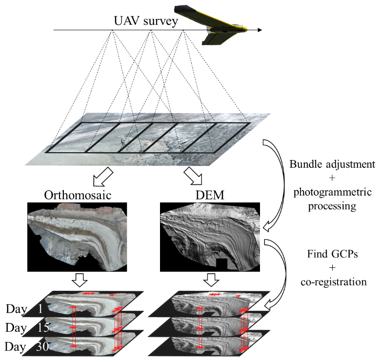
Figure 2Acquisition and processing chain used to derive the co-registered orthomosaics and DEMs.
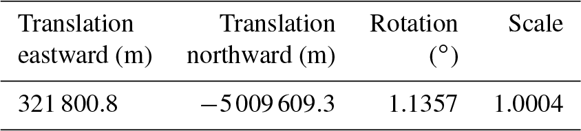
After co-registration, all final products (orthomosaics and DEMs) are in the reference frame of the bundle adjustment of 9 June 2017 (hereafter referred to as master bundle adjustment). This local reference frame is a realization of the WGS84 reference system (with Universal Transverse Mercator (UTM zone 32) projection) using code-only GPS data as input for referencing. The absence of ground control points (GCPs) and the use of consumer-grade GPS observations in the bundle adjustment procedure can result in meter-level geolocation errors and internal deformations of the master bundle adjustment (James and Robson, 2014; Gindraux et al., 2017). While the internal deformations of the local reference frame lead to relative measurement errors of small amplitude (on the order of 1∕1000; see Sect. 4.1 for details), the geolocation errors related to the absence of GCPs can impair comparisons with other datasets covering the same geographic area. To improve absolute georeferencing and to link our dataset with the Swiss national reference system, Table 2 provides the parameters of the affine transformation between the local reference frame of this dataset and the Swiss CH1903 – LV 03 reference system. This transformation has been estimated from 81 manual tie points identified in (1) the orthomosaic derived from the master bundle adjustment and (2) a 50 cm resolution orthomosaic of 2009 processed and georeferenced by the Swiss mapping agency swisstopo.
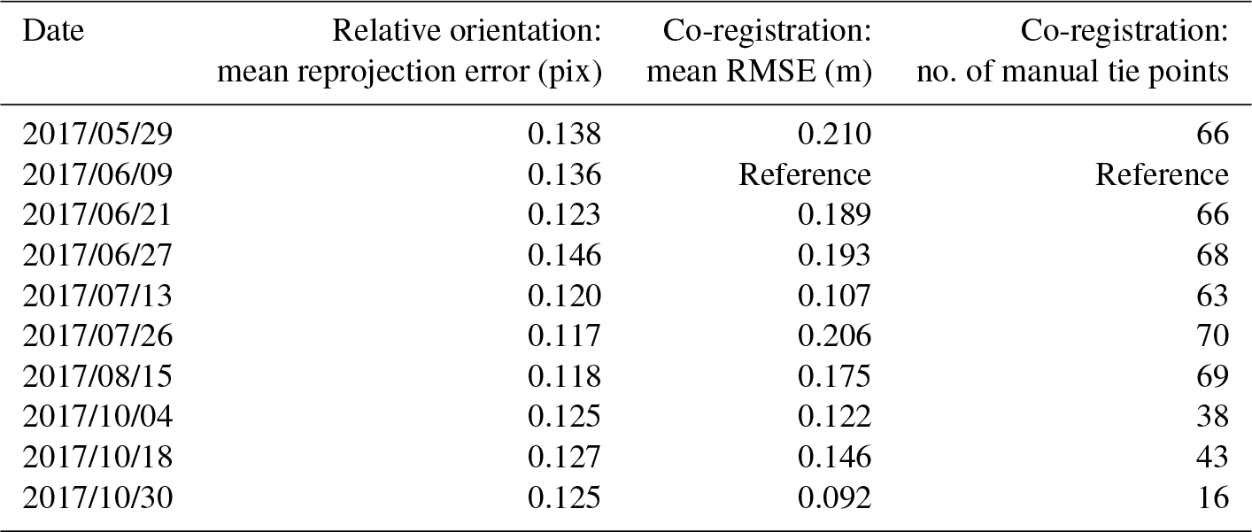
Table 2Parameters of the affine transformation between the Swiss reference system (CH1903 – LV03) and the local reference frame defined by the master bundle adjustment of 9 June 2017. Note that no shear nor reflection is considered. Locations of the manual tie points used to estimate the transformation parameters are shown in Fig. 4.
3.2 Surface displacement tracking: generation of MMs
Consecutive co-registered orthomosaics enable us to quantify horizontal displacements at the surface of the glacier. In the present dataset, this information about ice surface displacements is provided by the MMs (Fig. 3). In practice, a MM is an image that pairs the positions of similar ice patches at times t and t+dt (dt being the time span between consecutive acquisitions) (Fig. 2). The footprint of the MM is the overlap of the footprints of the orthomosaics at times t and t+dt. MMs inherit the spatial resolution of the original orthomosaics (i.e., 10 cm) and can therefore be used to directly relate any pixel of a given orthomosaic to its counterpart in the following orthomosaic (and therefore easily navigate within the whole dataset).
The MMs are obtained by image matching of pairs of orthomosaics. The orthomosaic at time t is taken as a reference, and for each pixel of the reference, a 51×51 pixel (5.1 m × 5.1 m) patch is extracted and searched for in the orthomosaic corresponding to the next session (time t+dt). To speed up the processing and avoid wrong matches with very distant patches, the homologous patch at time t+dt is searched for in a neighborhood with a 200-pixel (20 m) radius centered on the position of the original patch at time t whose size has been established based on prior knowledge about the approximate surface velocity of the Gorner Glacier. The criterion used to evaluate the similarity between both patches is the mean absolute error (MAE) between pixels computed on grayscale images (Liu and Zaccarin, 1993; Chuang et al., 2015). The MAE has been selected as the similarity score because it is fast to compute, especially on large images using convolutions. Its disadvantage is the sensitivity to illumination differences between consecutive orthoimages. However, in practice, no adverse effects have been observed, mostly because the images were acquired roughly at the same time of the day (between 11:30 and 16:00), and because the orthoimages used to generate the MMs are always separated by less than 1 month, which mitigates the illumination differences. The patch of the image t+dt leading to the lowest MAE with the original patch at time t is then considered the counterpart of the original patch. Finally, the displacements (in pixels) between the two patches along the east–west and the north–south directions are recorded into the MM. This operation is repeated for all possible patches in the reference orthomosaic. The MMs have been calculated using an open-source utility called MatchingMapMaker developed as part of this project, and made available along with the dataset (see Sect. 5.2 for code availability). The MatchingMapMaker tool has been designed to account for the specificities of UAV-based orthoimages, and in particular their very high resolution. To ensure the reliability of this utility, MMs have been benchmarked against horizontal displacement maps calculated using well-established image correlation algorithms, namely IMCORR (Scherler et al., 2008) and CIAS (Heid and Kääb, 2012). The results of this benchmark (see Sect. 5.2) show a very good agreement between horizontal displacement maps derived from MatchingMapMaker, IMCORR, and CIAS.
The raw MMs can be noisy due to the presence of outliers in the pattern matching procedure (speckled areas in the raw displacement maps in Fig. 3). These outliers originate from the dissimilarity between subsequent orthomosaics, due to, for example, changing shadows or changes at the glacier surface (snowfall, snow, or ice melting, etc.). To mitigate the impact of these outliers, we first locate them, then we mask the impacted areas (pink areas in Fig. 3), and finally we interpolate the remaining reliable displacements to fill the gaps generated by the mask. To limit the processing time, a simplistic outlier detection method based on signal processing has been preferred over more sophisticated approaches based on glacier physics (Maksymiuk et al., 2016). Unreliable areas in the raw MMs are assumed to be aggregates of pixels with spatially incoherent displacement values embedded in a matrix of displacements that vary smoothly in space (i.e., the reliable displacements). The borders of unreliable areas are detected as locations with strong spatial displacement gradients, with a detection threshold set to 15 cm of horizontal deformation per day. A mask of reliability is then created by setting the areas with a strong gradient to 0 and the remainder of the mask image to 1. The outlier areas (i.e., small aggregates of unreliable values) are then filtered out by applying the opening operator of mathematical morphology to this mask with a structuring element of the size 50×50 pixels. This operation leads to switch the value of the mask from 1 to 0 for all aggregates of pixels smaller than 50×50 pixels. Hence, we obtain a mask with 1 at locations with reliable displacements and 0 where the measured displacements are considered outliers. Finally, the values of the MM at masked locations are interpolated from the non-masked measurements using a bilinear interpolation. The selected procedure is iterative. At each iteration, it attributes to the masked values the mean of the reliable values in a 500-pixel neighborhood in the east–west and north–south directions. The values that remain masked after 10 iterations are considered to be too far from the informed areas to be filled and are set to −99 to denote no data. Figure 3 summarizes how MMs are derived from pairs of consecutive co-registered orthomosaics and filtered to remove outliers.
Because MMs pair the positions of similar ice patches between consecutive orthomosaics, they can be used to derive maps of the horizontal displacements occurring at the surface of the glacier. To this end, displacements from the masked MMs are converted to meters per day and resampled at a 5 m resolution to remove the dependence between neighboring locations that is introduced during the image matching procedure. Horizontal displacement maps at 5 m resolution are provided in addition to the full-resolution MMs in order to facilitate the use of the present dataset in the context of ice flow studies.
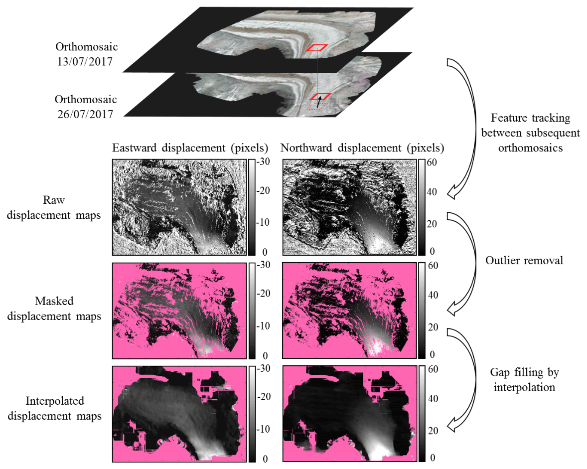
Figure 3Processing chain used to compute a MM between two subsequent orthomosaics. The procedure is illustrated for the 13 July 2017–26 July 2017 period. In displacement maps, masked areas are displayed in pink.
4.1 Bundle adjustment and co-registration
A first validation of this dataset can be performed by checking the relative orientation of the cameras during the bundle adjustment, as well as the co-registration of orthomosaics and DEMs. Processing reports detailing the quality of the bundle adjustment for each session are available along with the dataset (see Sect. 5.1).
Table 2 displays three indices summarizing the quality of both bundle adjustment steps. First, the mean reprojection error (in pixels) quantifies the mismatch in the raw images between the observed and the modeled position of tie points used during the relative orientation step. The sub-pixel level of errors (Table 2, column 2) ensures that the orientations of the camera are reliable. Next, the co-registration step is assessed by the mean root-mean-square error (RMSE) of manual tie point coordinates. This statistic measures the stability of manual tie point coordinates between different bundle adjustments. Under ideal conditions, the value of the mean RMSE on manual tie points should be close to the ground pixel resolution of the raw images (i.e., 7.3 to 8.8 cm) because an operator is able to identify points of interest with a pixel level precision. The slightly higher values obtained in the present case (9 to 21 cm, Table 2, column 3) can be due to the difficulty of precisely identifying manual tie points under changing environmental conditions (e.g., sunlight exposition or snow cover). The errors in manual tie point identification degrade the mean RMSE, but they are expected to have a mild impact on the co-registration itself because they are not correlated and tend to compensate for each other. Note that late in the season (i.e., for the last acquisition on 30 October) it became difficult to identify manual tie points due to strong shadows, hence the small number of manual tie points at that time.
Another important validation consists of assessing possible internal deformations within the local reference frame of the dataset. Figure 4a displays the residuals of the co-registration of the master bundle adjustment on a georeferenced orthoimage, which are a proxy for the internal deformations of the master bundle adjustment. The results show that the internal deformations have a meter-level amplitude (mean deformation =1.07 m; max deformation =2.83 m) and are smoothly spread over the area of interest due to the bundle adjustment procedure, which tends to distribute errors over space. It follows that, considering the extent of the study area (a few square kilometers), the relative error induced by the internal deformations of the local reference frame is on the order of 1∕1000. Thanks to the co-registration procedure, the internal deformations of all orthomosaics and DEMs are similar to the ones of the local reference frame defined by the master adjustment. When measuring changes at the surface of the glacier from the present dataset, the error related to internal deformations is therefore on the order of 1 ‰ of the measured distances. This results in relatively small absolute errors because the changes at the ice surface of the Gorner Glacier are of moderate amplitude (e.g., ice ablation reaches a few centimeters per day, and ice flows at less than 1 m d−1 in the ablation zone). For instance, in the case of horizontal velocity measurements, the order of magnitude of glacier displacement between two acquisition dates is 30 cm d d =4.2 m. It follows that the error in velocity due to internal deformations is 4.2 m d =0.3 mm d−1, which is very small in comparison with the amplitude of the ice surface velocity itself.
4.2 Orthomosaics and DEMs
In addition to the bundle adjustment, we also validate the final products of the photogrammetric processing (Fig. 4a), i.e., the co-registered orthomosaics and DEMs. To this end, individual orthomosaics and DEMs have first been visually checked to track the presence of artifacts. A careful examination of all products shows that the glaciated parts (Fig. 4b) as well as the neighboring ice-free areas (Fig. 4c) are well reconstructed in both orthomosaics and DEMs. On the edges of the area of interest artifacts can be present due to the low number of overlapping images in these areas (see the processing reports to identify them). This leads to unreliable photogrammetric reconstructions and in particular shear lines (Fig. 4d). Despite these relatively minor artifacts restricted to the edges of the surveyed area, all glaciated parts and nearby unglaciated margins are satisfyingly reconstructed in both orthomosaics and DEMs.
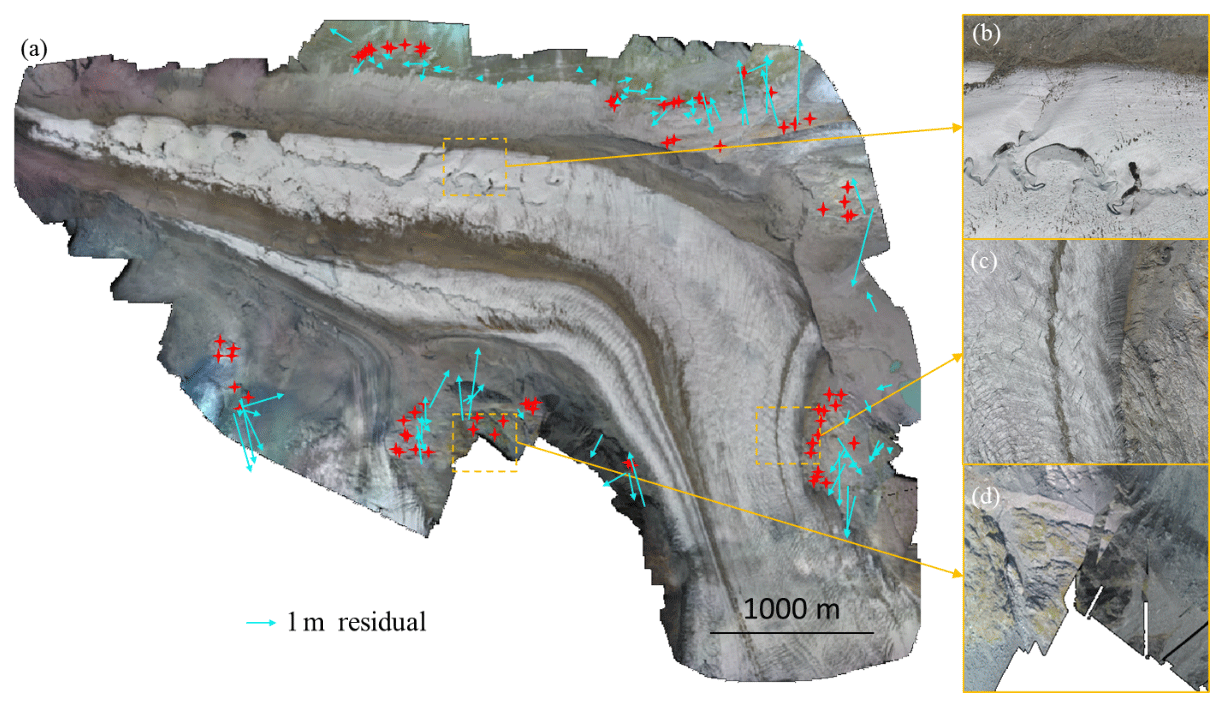
Figure 4Quality assessment of the orthomosaics. (a) Overview of one orthomosaic (15 August 2017). Red stars: manual tie points used for co-registration. Blue arrows: residuals after co-registration of the master bundle adjustment on a 50 cm resolution orthoimage acquired in 2009. The affine transformation described in Table 2 has been used for co-registration. (b–c) Examples of areas where the photogrammetric processing worked properly. (d) Example of area on the boundary of the domain where the photogrammetric processing produced artifacts (mostly shear lines).
4.3 MMs
In addition to the visual inspection of individual photogrammetric products, we also assess the quality of the co-registration procedure by quantifying in the MMs the stability of several areas that are most likely static, as well as the observed spatial patterns of glacier surface velocity. We select several validation locations on and off the glacier (Fig. 5) and compute their horizontal velocity by dividing the displacements recorded in the MMs by the time elapsed between the acquisitions. Note that in Fig. 5 the velocity is averaged over 10×10 m2 areas, corresponding to 10 000 single measurement points, centered on the validation points.
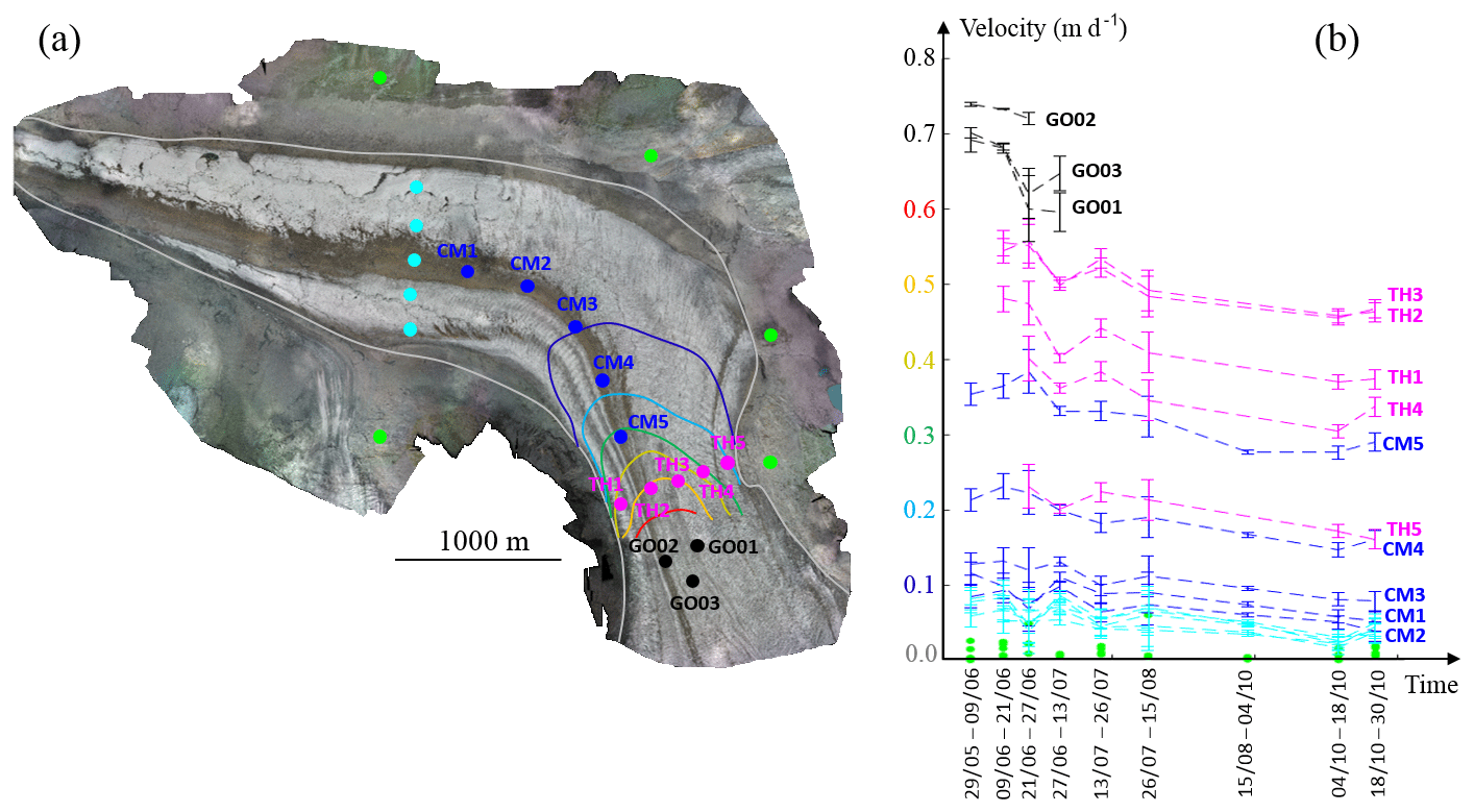
Figure 5Quality assessment of the MMs. (a) Locations of the validation points. The contour lines represent the horizontal surface velocity derived from the MM related to the period 13–26 July. (b) Observed horizontal surface velocities at validation locations. Error bars show 1σ errors. The errors reported for UAV-based velocities are empirical errors and are equal to the quadratic mean of velocities recorded at ice-free locations (green dots in b). The errors reported for GNSS-based velocities (i.e., at locations GO01, GO02, and GO03) are theoretical errors accounting for the uncertainty induced by the tilt of the support of GNSS receivers over time due to glacier movement.
Figure 5b displays the observed horizontal velocities in the domain for summer 2017. In the case of perfect photogrammetric processing, co-registration, and feature tracking, the apparent velocity of the ice-free areas (in green in Fig. 5) should be zero. While it is not exactly the case due to inherent processing errors and measurement noise, the mean velocity is very low (1.2 cm d−1 on average over the five ice-free validation locations), which reflects an appropriate processing. The observed patterns of glacier surface velocity are also in accordance with typical patterns of ice flow, such as velocities decreasing from the center of the glacier towards the edges (compare the velocity in TH3 and TH5) and higher velocities at steep parts of Grenz Glacier than on the flat tongue of Gorner Glacier (compare TH2 and CM5 to CM1). Finally, the velocities derived from UAV correspond to independent data collected by differential GNSS measurements a few hundred meters upstream of the area of interest (points GO01, GO02, and GO03 in Fig. 5). The higher velocity measured at the locations monitored by GNSS (points GO01–G003) compared to the downstream locations monitored by UAV (points TH1–TH3) is coherent with the increase in glacier velocity at the steeper upstream part of Grenz Glacier (approx. 13.5 % at GO02 compared to 7.5 % at TH2). Finally, the trend of deceleration over the course of the summer recorded by GNSS is in good agreement with the UAV-based velocities throughout the glacier.
5.1 Structure and availability of the dataset
All the data presented in this dataset are available in the following repository (Rep): https://zenodo.org/record/2630456, with the following DOI: https://doi.org/10.5281/zenodo.2630456 (Benoit et al., 2018).
The results of the photogrammetric processing, i.e., the orthomosaics and the DEMs, are available in the compressed folder Rep\Photogrammetric_Products.zip. Within this folder, the products are grouped in sub-folders by acquisition date using the following standard: 2017_mm_dd with “mm” the month and “dd” the day of acquisition. Finally, these sub-folders contain the following files:
-
2017_mm_dd_orthomosaic.tiff: contains the orthomosaic.
-
2017_mm_dd_dem.tiff: contains the DEM.
-
2017_mm_dd_report.pdf: contains the processing report (generated by Pix4D Mapper) that summarizes the quality of the photogrammetric processing for the date of interest.
The MMs are stored in the compressed folder Rep\Matching_Maps.zip. Within this folder, full-resolution MMs are stored in the \Full_resolution_Matching_Maps sub-folder. In this folder, individual maps are grouped in sub-folders named according to the acquisition date of the pair of subsequent orthomosaics used to generate the MM: 2017_mm_dd_2017_nn_ee with “mm” (resp. “dd”) and “nn” (resp. “ee”) the acquisition months (resp. days). These sub-folders contain the following files:
-
2017_mm_dd_2017_nn_ee_disp_Eastward: contains the MM of eastward displacements.
-
2017_mm_dd_2017_nn_ee_disp_Northward: contains the MM of northward displacements.
-
2017_mm_dd_2017_nn_ee__disp_mask: contains the mask of reliable displacements after filtering: 1 if the location corresponds to a reliable displacement, 0 otherwise.
In addition to the full-resolution MMs, displacement maps at 5 m resolution are stored in the \Final_Displacement_Maps sub-folder. Note that in contrast to the MMs, the displacement maps are in meters per day. Displacement maps follow the same file nomenclature as MMs, except the _Res5m suffix that allows us to distinguish displacement maps from MMs.
5.2 Code availability
The photogrammetric processing has been carried out using the proprietary software Pix4D Mapper, commercially available at https://pix4d.com/ (last access: 16 November 2018).
The MM have been computed using MATLAB routines written by Mathieu Gravey. The related utilities are freely available on the following repository: https://github.com/GAIA-UNIL/MatchingMapMaker (Gravey, 2018). The sub-repository Benchmarking_tests contains the results of benchmarking tests aiming at comparing the displacement maps computed by the MatchingMapMaker utility (i.e., MMs) with displacement maps computed by well-established glacier surface tracking algorithms, namely IMCORR (https://nsidc.org/data/velmap/imcorr.html, last access: 29 April 2019) and CIAS (https://www.mn.uio.no/geo/english/research/projects/icemass/cias/, last access: 29 April 2019). The sub-repository Similarity_score_tests contains the results of tests assessing the sensitivity of the MatchingMapMaker output to the similarity score used to define patch matches.
The present dataset compiles 10 UAV surveys of the Gorner Glacier carried out during summer 2017. Photogrammetric processing leads to a set of 10 cm resolution orthomosaics, DEMs, and glacier displacement maps for each acquisition date. This dataset can be used for change detection and quantification at the glacier surface, and in particular to investigate glacier surface dynamics at high temporal and spatial resolution.
AG, FH, and GM designed the experiment. AG, RV, II, BL, GP, and LB carried out the acquisitions. AG, RV, and LB performed the photogrammetric processing. MG, LB, and AG computed the matching maps. DG recorded differential GNSS data used for validation. LB wrote the paper with inputs from all authors.
The authors declare that they have no conflict of interest.
The authors are grateful to Philippe Limpach from ETH Zürich who processed the GNSS data.
This paper was edited by Reinhard Drews and reviewed by Bas Altena and one anonymous referee.
Aizen, V. B., Kuzmichenok, V. A., Surazakov, A. B., and Aizen, E. M.: Glacier changes in the central and northern Tien Shan during the last 140 years based on surface and remote-sensing data, Ann. Glaciol., 43, 202–213, 2006.
Baltsavias, E. P., Favey, E., Bauder, A., Bösch, H., and Pateraki, M.: Digital surface modelling by airborne laser scanning and digital photogrammetry for glacier monitoring, Photogramm. Rec., 17, 243–273, 2001.
Barrand, N. E., Murray, T., James, T. D., Barr, S. L., and Mills, J. P.: Optimizing photogrammetric DEMs for glacier volume change assessment using laser-scanning derived ground-control points, J. Glaciol., 55, 106–116, 2009.
Benoit, L., Dehecq, A., Pham, H., Vernier, F., Trouvé, E., Moreau, L., Martin, O., Thom, C., Pierrot-Deseilligny, M., and Briole, P.: Multi-method monitoring of Glacier d'Argentière dynamics, Ann. Glaciol., 56, 118–128, 2015.
Benoit, L., Gourdon, A., Vallat, R., Irarrazaval, I., Gravey, M., Lehmann, B., Prasicek, G., Gräff, D., Herman, F., and Mariethoz, G.: A high-frequency and high-resolution image time series of the Gornergletscher – Swiss Alps – derived from repeated UAV surveys, https://doi.org/10.5281/zenodo.2630456, 2018.
Berthier, E., Vincent, C., Magnússon, E., Gunnlaugsson, Á. Þ., Pitte, P., Le Meur, E., Masiokas, M., Ruiz, L., Pálsson, F., Belart, J. M. C., and Wagnon, P.: Glacier topography and elevation changes derived from Pléiades sub-meter stereo images, The Cryosphere, 8, 2275–2291, https://doi.org/10.5194/tc-8-2275-2014, 2014.
Berthier, E., Cabot, V., Vincent, C., and Six, D.: Decadal Region-Wide and Glacier-Wide Mass Balances Derived from Multi-Temporal ASTER Satellite Digital Elevation Models. Validation over the Mont-Blanc Area, Front. Earth Sci., 4, 63, https://doi.org/10.3389/feart.2016.00063, 2016.
Bhardwaj, A., Sam, L., Akanksha, Martín-Torres, F. J., and Kumar, R.: UAVs as remote sensing platform in glaciology: Present applications and future prospects, Remote Sens. Environ., 175, 196–204, 2016.
Brun, F., Wagnon, P., Berthier, E., Shea, J. M., Immerzeel, W. W., Kraaijenbrink, P. D. A., Vincent, C., Reverchon, C., Shrestha, D., and Arnaud, Y.: Ice cliff contribution to the tongue-wide ablation of Changri Nup Glacier, Nepal, central Himalaya, The Cryosphere, 12, 3439–3457, https://doi.org/10.5194/tc-12-3439-2018, 2018.
Chen, J. and Funk, M.: Mass balance of Rhonegletscher during 1882/83–1986/87, J. Glaciol., 36, 199–209, 1990.
Chuang, M.-C., Hwang, J.-N., Williams, K., and Towler, R.: Tracking Live Fish from Low-Contrast and Low-Frame-Rate Stereo Videos, IEEE T. Circ. Syst. Vid., 25, 167–179, 2015.
Cuffey, K. M. and Paterson, W. S. B.: The physics of glaciers, Elsevier Science, 2010.
Dehecq, A., Gourmelen, N., and Trouvé, E.: Deriving large-scale glacier velocities from a complete satellite archive: Application to the Pamir–Karakoram–Himalaya, Remote Sens. Environ., 162, 55–66, 2015.
Dunse, T., Schuler, T. V., Hagen, J. O., and Reijmer, C. H.: Seasonal speed-up of two outlet glaciers of Austfonna, Svalbard, inferred from continuous GPS measurements, The Cryosphere, 6, 453–466, https://doi.org/10.5194/tc-6-453-2012, 2012.
Fugazza, D., Scaioni, M., Corti, M., D'Agata, C., Azzoni, R. S., Cernuschi, M., Smiraglia, C., and Diolaiuti, G. A.: Combination of UAV and terrestrial photogrammetry to assess rapid glacier evolution and map glacier hazards, Nat. Hazards Earth Syst. Sci., 18, 1055–1071, https://doi.org/10.5194/nhess-18-1055-2018, 2018.
Gabbud, C., Micheletti, N., and Lane, S. N.: Lidar measurement of surface melt for a temperate Alpine glacier at the seasonal and hourly scales, J. Glaciol., 61, 963–974, 2015.
Gindraux, S., Boesch, R., and Farinotti, D.: Accuracy assessment of digital surface models from Unmanned Aerial Vehicles' imagery on glaciers, Remote Sensing, 9, 186, https://doi.org/10.3390/rs9020186, 2017.
Gravey, M.: MatchingMapMaker utilities, available at: https://github.com/GAIA-UNIL/MatchingMapMaker (last access: 29 April 2019), 2018.
Heid, T. and Kääb, A.: Evaluation of existing image matching methods for deriving glacier surface displacements globally from optical satellite imagery, Remote Sens. Environ., 118, 339–355, 2012.
Herman, F., Anderson, B., and Leprince, S.: Mountain glacier velocity variation during a retreat/advance cycle quantified using sub-pixel analysis of ASTER images, J. Glaciol., 57, 197–207, 2011.
Huss, M., Hock, R., Bauder, A., and Funk, M.: Conventional versus reference-surface mass balance, J. Glaciol., 58, 278–286, 2012.
Immerzeel, W. W., Kraaijenbrink, P. D. A., Shea, J. M., Shrestha, A. B., Pellicciotti, F., Bierkens, M. F. P., and de Jong, S. M.: High-resolution monitoring of Himalayan glacier dynamics using unmanned aerial vehicles, Remote Sens. Environ., 150, 93–103, 2014.
James, M. R. and Robson, S.: Mitigating systematic error in topographic models derived from UAV and ground-based image networks, Earth Surf. Proc. Land., 39, 1413–1420, 2014.
Jouvet, G., Weidmann, Y., Seguinot, J., Funk, M., Abe, T., Sakakibara, D., Seddik, H., and Sugiyama, S.: Initiation of a major calving event on the Bowdoin Glacier captured by UAV photogrammetry, The Cryosphere, 11, 911–921, https://doi.org/10.5194/tc-11-911-2017, 2017.
Kääb, A., Berthier, E., Nuth, C., Gardelle, J., and Arnaud, Y.: Contrasting patterns of early twenty-first-century glacier mass change in the Himalayas, Nature, 488, 495–498, 2012.
Kraaijenbrink, P., Meijer, S. W., Shea, J. M., Pellicciotti, F., De Jong, S. M., and Immerzeel, W. W.: Seasonal surface velocities of a Himalayan glacier derived by automated correlation of unmanned aerial vehicle imagery, Ann. Glaciol., 57, 103–113, 2016.
Liu, B. and Zaccarin, A.: New Fast Algorithms for the Estimation of Block Motion Vectors, IEEE T. Circ. Syst. Vid., 3, 148–157, 1993.
Maksymiuk, O., Mayer, C., and Stilla, U.: Velocity estimation of glaciers with physically-based spatial regularization – Experiments using satellite SAR intensity images, Remote Sens. Environ., 172, 190–204, 2016.
Mertes, J. R., Gulley, J. D., Benn, D. I., Thompson, S. S., and Nicholson, L. I.: Using structure-from-motion to create glacier DEMs and orthoimagery from historical terrestrial and oblique aerial imagery, Earth Surf. Proc. Land., 42, 2350–2364, 2017.
Piermattei, L., Carturan, L., and Guarnieri, A.: Use of terrestrial photogrammetry based on structure-from-motion for mass balance estimation of a small glacier in the Italian alps, Earth Surf. Proc. Land., 40, 1791–1802, 2015.
Racoviteanu, A. and Williams, M. W.: Decision tree and texture analysis for mapping debris-covered glaciers in the Kangchenjunga area, Eastern Himalaya, Remote Sensing, 4, 3078–3109, 2012.
Ramirez, E., Francou, B., Ribstein, P., Descloitres, M., Guérin, R., Mendoza, J., Gallaire, R., Pouyaud, B., and Jordan, E.: Small glaciers disappearing in the tropical Andes: a case-study in Bolivia: Glaciar Chacaltaya (16∘ S), J. Glaciol., 47, 187–194, 2001.
Riesen, P., Sugiyama, S., and Funk, M.: The influence of the presence and drainage of an ice-marginal lake on the flow of Gornergletscher, Switzerland, J. Glaciol., 56, 278–286, 2010.
Rippin, D. M., Pomfret, A., and King, N.: High resolution mapping of supra-glacial drainage pathways reveals link between micro-channel drainage density, surface roughness and surface reflectance, Earth Surf. Proc. Land., 40, 1279–1290, 2015.
Rossini, M., Di Mauro, B., Garzonio, R., Baccolo, G., Cavallini, G., Mattavelli, M., De Amicis, M., and Colombo, R.: Rapid melting dynamics of an alpine glacier with repeated UAV photogrammetry, Geomorphology, 304, 159–172, 2018.
Ryan, J. C., Hubbard, A. L., Box, J. E., Todd, J., Christoffersen, P., Carr, J. R., Holt, T. O., and Snooke, N.: UAV photogrammetry and structure from motion to assess calving dynamics at Store Glacier, a large outlet draining the Greenland ice sheet, The Cryosphere, 9, 1–11, https://doi.org/10.5194/tc-9-1-2015, 2015.
Scherler, D., Leprince, S., and Strecker, M. R.: Glacier-surface velocities in alpine terrain from optical satellite imagery – Accuracy improvement and quality assessment, Remote Sens. Environ., 112, 3806–3819, 2008.
Sold, L., Huss, M., Machguth, H., Joerg, P. C., Leysinger Vieli, G., Linsbauer, A., Salzmann, N., Zemp, M., and Hoelzle, M.: Mass balance re-analysis of Findelengletscher, Switzerland; benefits of extensive snow accumulation measurements, Front. Earth Sci., 4, 18, https://doi.org/10.3389/feart.2016.00018, 2016.
Sugiyama, S., Bauder, A., Riesen, P., and Funk, M.: Surface ice motion deviating toward the margins during speed-up events at Gornergletscher, Switzerland, J. Geophys. Res.-Earth, 115, F03010, https://doi.org/10.1029/2009JF001509, 2010.
Vallet, J., Panissod, F., Strecha, C., and Tracol, M.: Photogrammetric performance of an ultra light weight swinglet “UAV”, International Archives of the Photogrammetry, Remote Sensing and Spatial Information Sciences, XXXVIII-1, 253–258, 2011.
Werder, M. A. and Funk, M.: Dye tracing a jökulhlaup: II. Testing a jökulhlaup model against flow speeds inferred from measurements, J. Glaciol., 55, 899–908, 2009.
Werder, M. A., Loye, A., and Funk, M.: Dye tracing a jökulhlaup: I. subglacial water transit speed and water-storage mechanism, J. Glaciol., 55, 889–898, 2009.
Werder, M. A., Hewitt, I. J., Schoof, C. G., and Flowers, G. E.: Modeling channelized and distributed subglacial drainage in two dimensions, J. Geophys. Res.-Earth, 118, 2140–2158, 2013.
Whitehead, K., Moorman, B. J., and Hugenholtz, C. H.: Brief Communication: Low-cost, on-demand aerial photogrammetry for glaciological measurement, The Cryosphere, 7, 1879–1884, https://doi.org/10.5194/tc-7-1879-2013, 2013.
Yang, K. and Smith, L. C.: Supraglacial Streams on the Greenland Ice Sheet Delineated From Combined Spectral – Shape Information in High-Resolution Satellite Imagery, IEEE Geosci. Remote S., 10, 801–805, 2012.