A comprehensive global oceanic dataset of helium isotope and tritium measurements

Tritium and helium isotope data provide key information on ocean circulation, ventilation, and mixing, as well as the rates of biogeochemical processes and deep-ocean hydrothermal processes. We present here global oceanic datasets of tritium and helium isotope measurements made by numerous researchers and laboratories over a period exceeding 60 years. The dataset's DOI is https://doi.org/10.25921/c1sn-9631, and the data are available at https://www.nodc.noaa.gov/ocads/data/0176626.xml (last access: 15 March 2019) or alternately http://odv.awi.de/data/ocean/jenkins-tritium-helium-data-compilation/ (last access: 13 March 2019) and includes approximately 60 000 valid tritium measurements, 63 000 valid helium isotope determinations, 57 000 dissolved helium concentrations, and 34 000 dissolved neon concentrations. Some quality control has been applied in that questionable data have been flagged and clearly compromised data excluded entirely. Appropriate metadata have been included, including geographic location, date, and sample depth. When available, we include water temperature, salinity, and dissolved oxygen. Data quality flags and data originator information (including methodology) are also included. This paper provides an introduction to the dataset along with some discussion of its broader qualities and graphics.

1 Introduction

The global oceanic distributions of tritium (³H, a radioactive isotope of hydrogen with a half-life of 12.3 years), its daughter product ³He, and helium isotopes in general arise from the complicated interplay of ocean ventilation, circulation, and mixing, with the hydrologic cycle, air–sea exchange, and geological volatile input. Observations of the delivery of tritium to the ocean and its redistribution are a useful tool for diagnosing gyre- and basin-scale ventilation and circulation (Doney et al., 1992; Doney and Jenkins, 1994; Dorsey and Peterson, 1976; Dreisigacker and Roether, 1978; Fine and Östlund, 1977; Fine et al., 1987, 1981; Jenkins et al., 1983; Jenkins and Rhines, 1980; Michel and Suess, 1975; Miyake et al., 1975; Östlund, 1982; Sarmiento, 1983; Weiss and Roether, 1980; Weiss et al., 1979).

In shallow waters, away from seafloor hydrothermal vents, the combination of tritium and ³He may be used to determine the time elapsed since a water parcel was at the sea surface, making it a useful tool for diagnosing ventilation and circulation on seasonal through decade timescales (Jenkins, 1987, 1998, 1977). The ingrowth and evasion of tritiugenic ³He from the thermocline is also useful as a flux gauge for constraining the rate of nutrient return to the ocean surface (Jenkins, 1988; Jenkins and Doney, 2003; Stanley et al., 2015) as well as upwelling in coastal regions (Rhein et al., 2010). Finally, the distribution of helium isotopes in the deep sea provides important quantitative constraints on the impact of submarine hydrothermal venting on many elements because the global hydrothermal helium flux is well known (Bianchi et al., 2010; Holzer et al., 2017; Schlitzer, 2016). This makes ³He useful as a flux gauge (German et al., 2016; Jenkins et al., 1978, 2018a; Lupton and Jenkins, 2017; Resing et al., 2015; Roshan et al., 2016). Consequently, there have been numerous measurements of these properties over the years, particularly under the aegis of major observational programs like GEOSECS (Bainbridge et al., 1987), TTO (Jenkins and Smethie, 1996), WOCE (http://www.nodc.noaa.gov/woce/wdiu/diu_summaries/whp/index.htm, last access: 1 April 2019), CLIVAR (http://www.clivar.org, last access: 1 April 2019), GO-SHIP (http://www.go-ship.org, last access: 1 April 2019), and GEOTRACES (http://www.geotraces.org, last access: 1 April 2019). It seems valuable to assemble all existing data, including those measured prior to and outside of these programs, along with appropriate metadata, in one place to facilitate further use and analysis. This is a report of these efforts.

2 Methods

2.1 Tritium measurement methodology

There are at present three distinct methods for the determination of tritium in water samples: direct measurement of tritium abundance by accelerator mass spectrometry (AMS), radioactive counting of tritium decay rate, and the daughter product (³He) ingrowth method. The first method (AMS) has not been used for the measurement of environmental tritium levels but is better suited to measuring high tritium concentrations in small samples, largely for biomedical tracer research (Brown et al., 2005; Chiarappa-Zucca et al., 2002; Glagola et al., 1984; Roberts et al., 2000). The second method usually involves isotopic enrichment of hydrogen from the water samples, either by electrolysis (e.g., Östlund and Werner, 1962) or thermal diffusion (Israel, 1962) followed by low-level radioactive counting, either by liquid scintillation (Momoshima et al., 1983) or gas proportional counting (Bainbridge et al., 1961). Measurements are made relative to prepared standards (Unterweger et al., 1980), and accuracy appears to be limited by the reproducibility of the enrichment process to 3 %–10 % (Cameron, 1967).

The third method, ³He ingrowth, is a three-step method. First, it involves degassing of a quantity (∼1 to 1000 mL) of water to remove all dissolved helium. Second, the degassed water is stored in a helium leak-tight container (usually low-He-permeability aluminosilicate glass or metal) for a period of several weeks to a year or more. Experience indicates that it is necessary to shelter the stored samples from cosmic rays since there is a latitude-dependent cosmogenic ³He production rate that masquerades as “tritium signal” (Lott and Jenkins, 1998). Finally, the ingrown ³He is extracted from the water sample and mass spectrometrically analyzed (Clarke et al., 1976; Ludin et al., 1997). The last method, although it involves a potentially lengthy incubation period, is chemically simpler and does not involve isotopic enrichment steps. As such, it offers intrinsically greater accuracy (limited by standardization of the mass spectrometer, typically better than 1 %) and a lower ultimate detection limit (Jenkins et al., 1983; Lott and Jenkins, 1998).

2.2 Helium isotope measurement methodology

Water samples are usually drawn from Niskin bottles into a helium leak-tight container either for shipboard (Lott and Jenkins, 1998; Roether et al., 2013) or shore-based gas extraction. The latter involves either clamped (Weiss, 1968) or crimped copper tubing (Young and Lupton, 1983). The extracted gases are subsequently purified and concentrated, usually cryogenically (Lott, 2001; Lott and Jenkins, 1984; Ludin et al., 1997), and expanded into a mass spectrometer for isotopic analysis. While time-of-flight mass spectrometry has been used (Mamyrin, 2001; Mamyrin et al., 1970), most oceanic helium isotope measurements have been made using multi-collector magnetic sector instruments (whereby ions are electrostatically accelerated and deflected by a magnetic field, e.g., Bayer et al., 1989; Clarke et al., 1969; Lott and Jenkins, 1998, 1984; Ludin et al., 1997). Measurements are typically standardized to marine air and corrected for any sample-size-dependent ratio effects determined by measurement of different-sized air aliquots. Depending on the amount of tritium in the water and the length of time a water sample is stored prior to gas extraction, it is generally necessary to correct the ³He∕⁴He results for decay of tritium during storage. For very deep and old samples, e.g., at 3000 m in the North Pacific, where tritium concentrations are very low, this correction may be inconsequential.

2.3 Helium and neon concentration measurements

To make full use of the helium isotopic ratio measurements, one needs to know at least the concentration of helium in the samples as well. This allows investigators to calculate the actual concentration of both ³He and ⁴He in samples and, with some assumptions, to estimate the amount of non-atmospheric ³He – whether it be from tritium decay or hydrothermal input – and ⁴He. The estimate can be further improved with knowledge of neon concentrations. Since neon is similar to helium in terms of its solubility in seawater and there are no known significant non-atmospheric sources of neon in the ocean, its concentration is a direct tracer of processes like air bubble injection at the sea surface. As an example, we show in Fig. 1 the relationship between the helium and neon saturation anomalies¹ for approximately 2000 near-surface samples. The saturation anomalies range from significantly below zero to as much as 10 %–15 %. The negative values may arise from lower barometric pressures or air–sea disequilibrium during cooling. However, there may be systematic offsets due to laboratory standardization as well. The higher values may also reflect such biases but also may be due to air bubble entrapment during sampling at sea. The solid line in Fig. 1 represents a type-II linear regression of the data and has a slope of near unity, which is expected given the similarity of the two gases. However, the slope is greater than the precise ratio expected (0.8 to 0.9 depending on temperature) based on their solubilities and atmospheric abundances, possibly due to differing air–sea exchange rates. Consideration must be given to these and other factors when using this data (e.g., Fuchs et al., 1987; Roether et al., 1998).

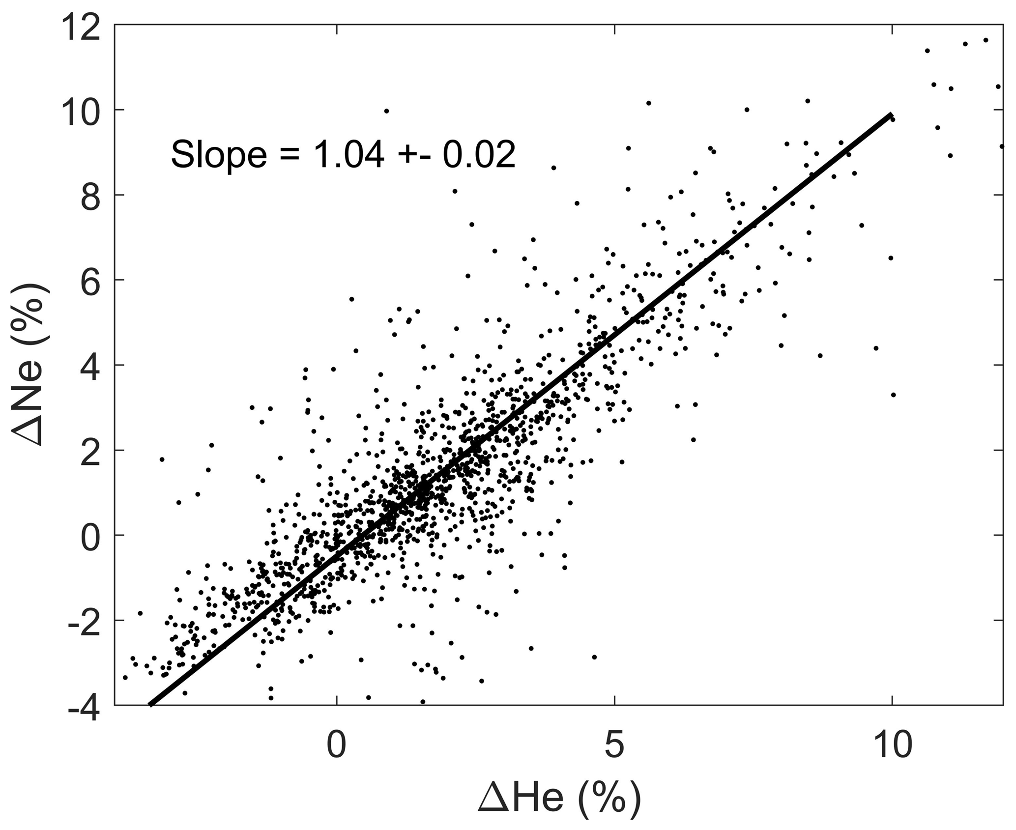
Figure 1 A scatter plot of helium and neon saturation anomalies for nearly 2000 near-surface (<20 m depth) samples from the dataset. The solid line is a type-II linear regression of the data.

Helium and neon concentration measurements are typically made by mass spectrometric peak height manometry, that is, by comparison of major isotope ion currents (⁴He⁺ and ²⁰Ne⁺) between the unknown to helium and neon derived from an aliquot of marine air. The air aliquot size is determined from a knowledge of the barometric pressure, relative humidity, and temperature at which the previously evacuated air standard reservoir was filled and the volume of the aliquot. Generally the ion current is assumed to be a linear function of the sample size (number of atoms) over some narrow range but also can be corrected by construction of a standard curve using different sized aliquots. Some measurements (notably the GEOSECS expedition) were made by splitting the gas extracted from the water sample and measuring the helium and neon contents separately using isotope dilution (with ³He and ²²Ne spikes).

2.4 Data organization

We have compiled a comprehensive dataset consisting of helium isotope and tritium measurements in oceanic waters made by numerous laboratories over the past 6 decades. The dataset includes ∼60 000 tritium and ∼63 000 helium isotope measurements, ∼57 000 dissolved helium concentrations, and ∼34 000 dissolved neon concentrations in ocean water taken from 1952 to 2015 (for tritium) and from 1967 to 2015 for helium. In addition to “spot sampling”, there are ∼380 cruises, with sampling from >5400 locations for tritium and ∼5600 locations for helium. The helium data are from 8 different laboratories and the tritium data from 15 laboratories worldwide. In addition to including measurement uncertainties, a data quality flag, and data source, each data point is accompanied by location (latitude, longitude, depth) and time (decimal year) of sampling. When available, water temperature, salinity, and dissolved oxygen measurements are included.

A number of the earliest measurements were obtained from publications. In those cases, the publication source is given. If the data were transcribed from tables, the table number and page is also given. In the event that the data were only available graphically, a computer program to digitize the data from plots was used, and in the rare cases in which graph quality was sufficiently poor to degrade the precision of the data, the uncertainties were commensurately increased to reflect it. Where data had been assigned a Digital Object Identifier (DOI), this is also included.

Table 1 Fields (columns) in the main data table.

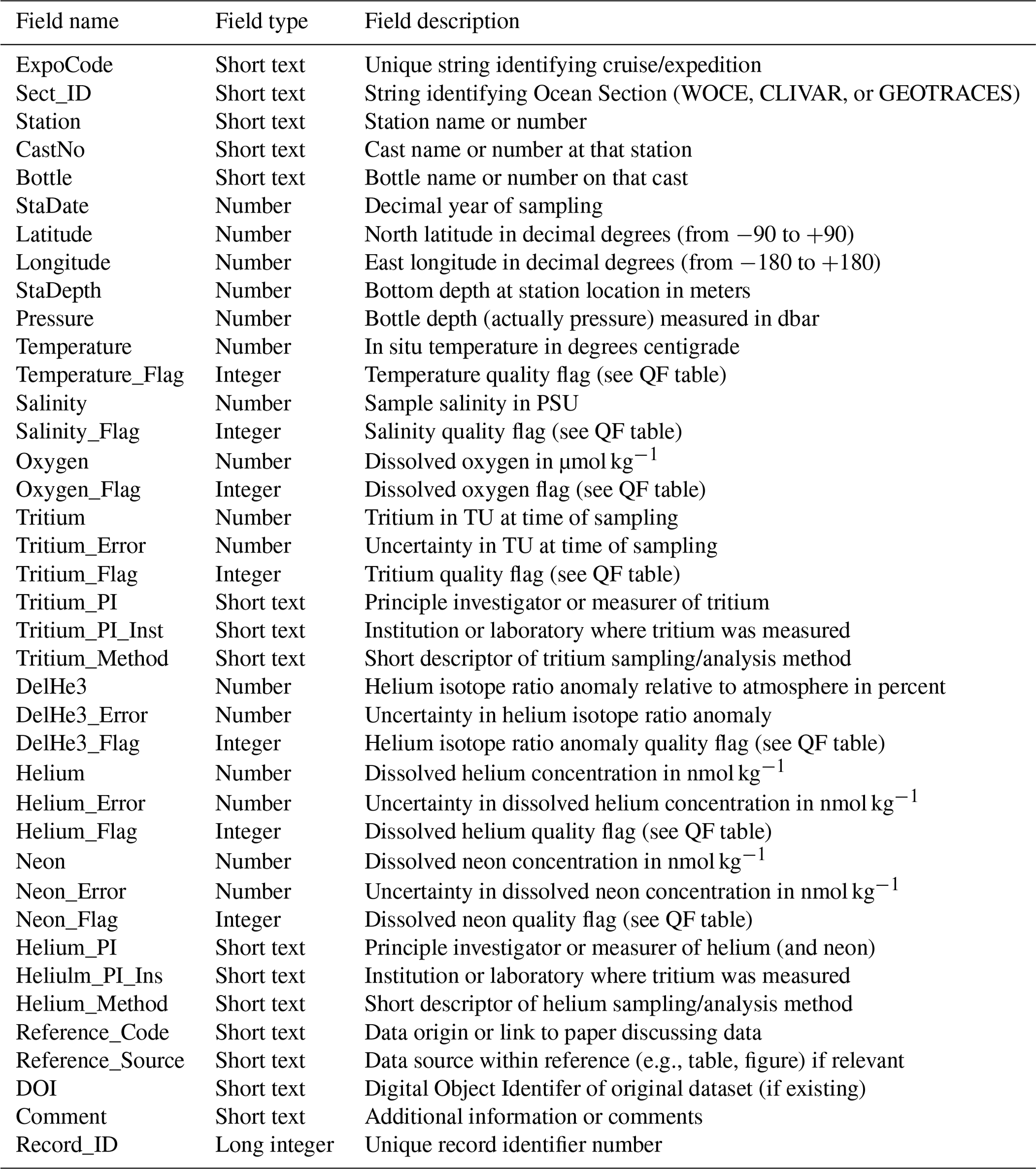
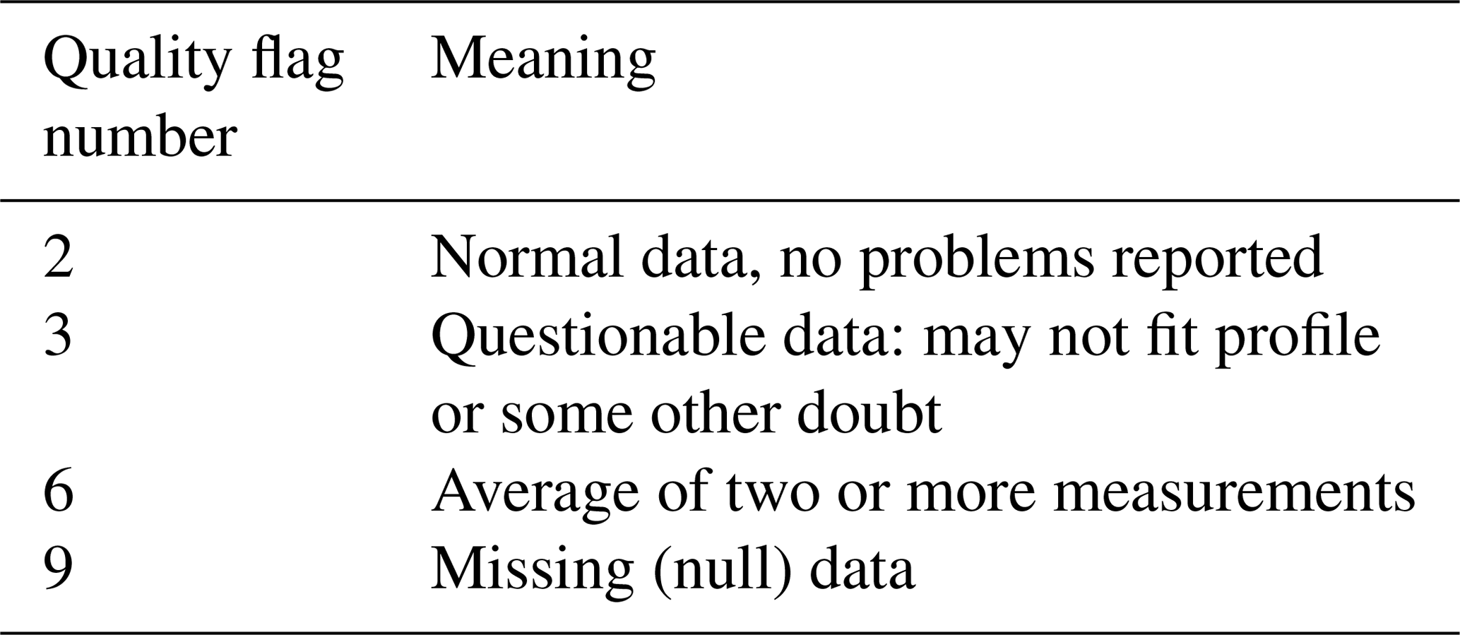
The dataset (provided in several digital formats described below) consists of three tables. The REFERENCES table is a list of the data sources keyed by the text variable “Reference_Code” found in the main data table. This provides attribution or more information regarding the data origin. The METHODS table provides a more complete description of the fields “Tritium_Method” and “Helium_Method” in the main data table. This is intended to provide useful interpretive information regarding how the sampling and/or measurements were accomplished. The main data table fields are described in Table 1. Most data fields have an associated quality flag field whose meaning is summarized in Table 2. Following WOCE ocean data convention, normal acceptable data are associated with a quality flag of 2, whereas questionable data have a flag of 3. Results obtained by averaging two or more replicates are signified with a flag of 6. When fields are missing for a given record, the data are entered as -999 and the corresponding quality flag is 9. The tritium, helium, helium isotope, and neon data also have an associated uncertainty field (e.g., “Tritium_Error”), which is the estimated uncertainty in the data points. This is either provided by the data measurer or an estimate based on described procedures and can vary greatly between methods and laboratories, so the user is advised to be aware of this value.

Table 2 Quality flag meaning.

In the spirit of the WOCE, CLIVAR, and GO-SHIP² convention, the combination of ExpoCode, Station, CastNo, and Bottle should uniquely define a sample. That is, no two data records should have the same combination of these values. This has been followed with most of the information here: when a sample's station, cast, or bottle number were not provided (in the case of literature data), arbitrary but unique numbers were assigned. In order to supplement this identification, we added a unique integer record ID number.

2.5 Data formats and availability

The dataset's DOI is https://doi.org/10.25921/c1sn-9631 (Jenkins et al., 2018b). The data are available for download from the U.S. National Oceanic and Atmospheric Administration's National Centers for Environmental Information website at https://www.nodc.noaa.gov/ocads/data/0176626.xml or alternately http://odv.awi.de/data/ocean/jenkins-tritium-helium-data-compilation/ in a number of formats. For maximum flexibility, we suggest one of the following three database formats: Microsoft Access^®, PostgreSQL, or ODV (Ocean Data View). In addition, the three tables are available as four files (the main data table is split into two to avoid spreadsheet row-number limitations) in Microsoft Excel^® or as comma-separated plain text files. The data are also available in NetCDF format. Finally, the data table is available for download as a MATLAB^® binary data file.

3 Scope and nature of the dataset

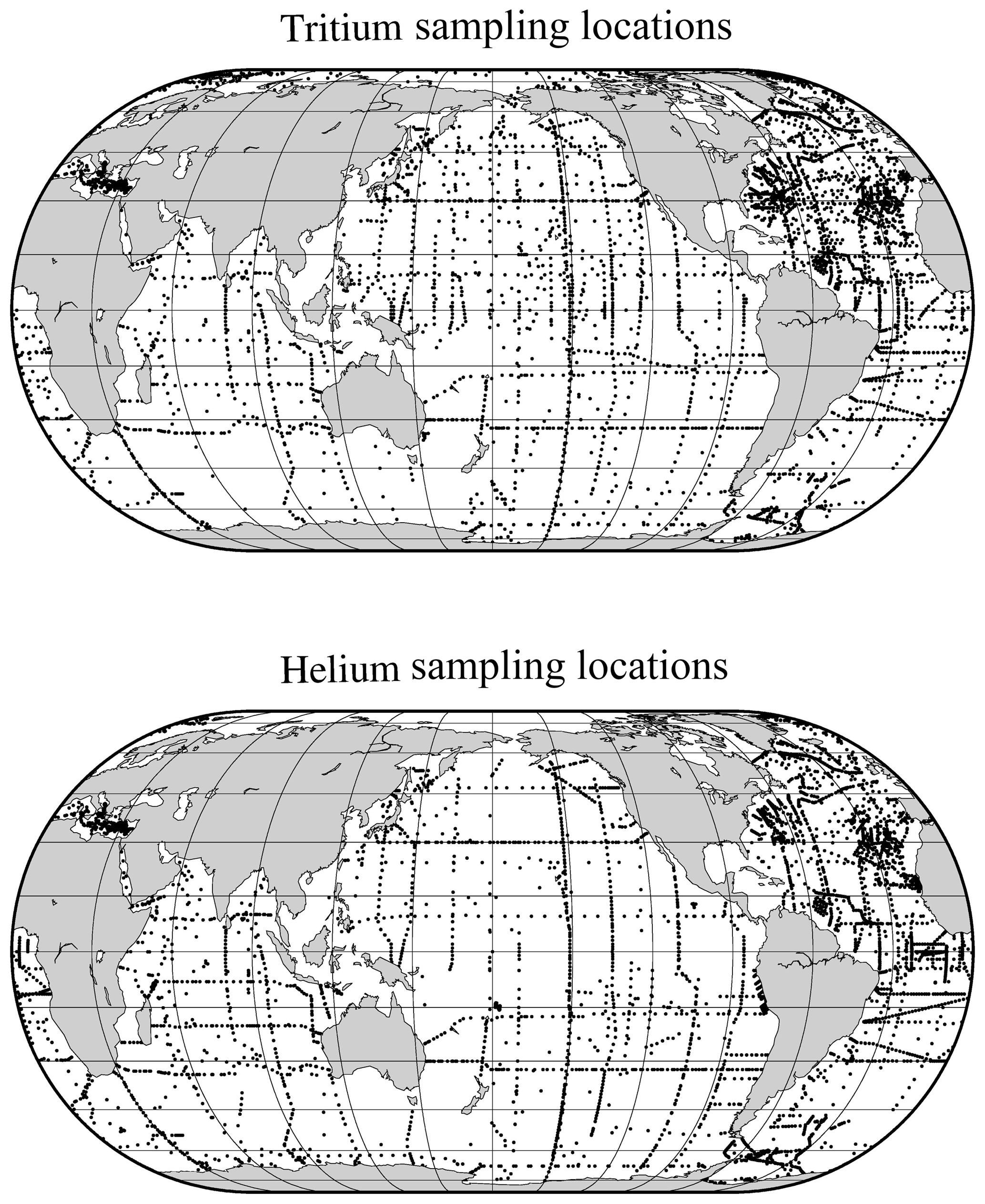
We provide some graphics to indicate the scope and nature of the data holdings. These include time histories of analyses per year for both types of measurements (Fig. 2) and maps of sampling locations (Fig. 3). The intent is to provide a broad overview of the character of the datasets while not overinterpreting its details and features.

The temporal distribution of oceanic tritium measurements begins in the early 1950s with the development of enrichment and counting capabilities suitable for environmental levels, the recognition of the existence of cosmogenic tritium production (Cornog and Libby, 1941; Currie et al., 1956; Grosse et al., 1951; Kaufman and Libby, 1954; Libby, 1946), and the desire to measure its distribution in the hydrologic cycle. The advent of atmospheric thermonuclear tests in the 1950s and early 1960s dwarfed the natural global inventory (Weiss and Roether, 1980), which motivated an increase in oceanic measurements in the 1960s. The initiation of global ocean chemistry, hydrographic, and tracer survey efforts (especially GEOSECS³) further increased this activity. A final boost to tritium measurement rates occurred with the development of the ³He regrowth method (Clarke et al., 1976) coupled with even more ambitious global surveys (such as WOCE, CLIVAR, and GO-SHIP).

Figure 2 Time distributions of annual tritium (a) and helium (b) measurements.

Figure 3 Tritium and helium sample locations.

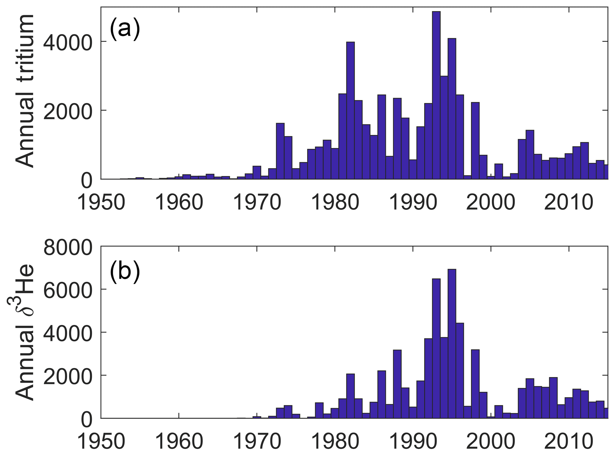
The helium sampling time history was basically initiated and motivated by the discovery of primordial ³He injection into the deep waters (Clarke et al., 1969), which drove the inclusion of helium isotope measurements in the GEOSECS program. It was quickly realized that the existence of tritiugenic ³He (that produced by the in situ decay of tritium) offered the potential for a dating tool as well (Jenkins et al., 1972; Jenkins and Clarke, 1976), which spurred on continued helium isotope measurements in the global surveys. These were enabled by a number of laboratories coming “online” in the 1970s and 1980s.

The tritium and helium sampling locations shown in Fig. 3 are dominated by the global survey programs' cruise tracks, but also include a number of ocean island monitoring sites (especially for tritium). One difference in the two maps is the extra tritium sampling in the Arctic, perhaps largely driven by H. Göte Östlund's motivation to exploit this isotope's potential in studying the Arctic fresh water system (Östlund, 1982).

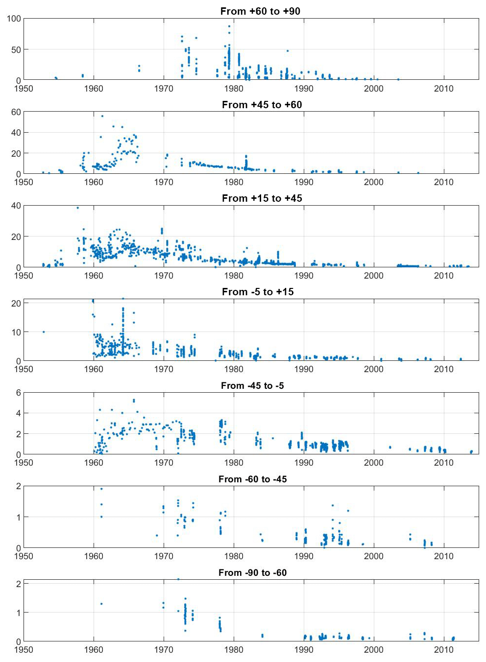
Figure 4 Global ocean surface water (depth <50 m) tritium concentrations (in TU) for selected latitude bands.

It is well known that the delivery of bomb tritium to the ocean was a reflection of the distribution of the atmospheric tests and occurred in two principle modes: a dominant pulse-like injection in the Northern Hemisphere and a much smaller more “diffuse” input into the Southern Hemisphere (Doney et al., 1992). The former mode was dominated by the early 1960s American and USSR tests that occurred just prior to the 1963 Partial Test Ban Treaty, while the southern hemispheric tests were carried out predominantly by the UK and France. Weiss and Roether (1980) estimated the delivery of approximately 1500 GCi to the Northern Hemisphere and 480 GCi to the Southern Hemisphere by the end of 1972. The latitudinal trends can be seen in Fig. 4, which is a plot of near-surface (<50 m depth) water tritium concentrations vs. time for a number of latitude bands. Most striking is the northward increase in the concentration (y-axis) ranges. The time–latitude trends in Fig. 4 reflect this globally asymmetric delivery, but much of the structure caused by regional variations in atmospheric input and ocean circulation may be masked due to conflating major ocean basins in the groupings.

As a transient tracer, tritium offers an opportunity to visualize the ventilation of deep waters on decade to century timescales. Benchmark observations of water column tritium concentrations during the GEOSECS Atlantic Expedition reveal North Atlantic deep water formation in a graphic manner (Östlund et al., 1974). The evolution of the tritium distributions is also valuable as they penetrate the subtropical thermocline and also intermediate and deep waters. Figure 5 shows four snapshots of tritium distributions on a section along approximately 52^∘ W in the North Atlantic between the South American and North American coasts (see map inset). Tritium concentrations are decay-corrected to a common midpoint in time (1997) for comparison. While the last three occupations are conveniently along the same cruise track (courtesy of WOCE, CLIVAR, and GO-SHIP), the first is a composite from several cruises of opportunity taken over an approximately 1-year period at roughly the same longitude. One can readily see the downward propagation and ultimate dispersion of the bomb tritium pulse within the main thermocline (the upper 1000 m), and the progressive ingrowth of tritium in the intermediate layer (1500–2500 m depth) and in the bottom layers (∼4000 m) is striking. One can also see the repartitioning of tritium inventories in the upper waters, both due to vertical exchange and ventilation but also due to the continued accumulation of this bomb fallout isotope at subtropical latitudes (similar to bomb radiocarbon, as observed by Broecker et al., 1995) from more tritium-rich waters to the north.

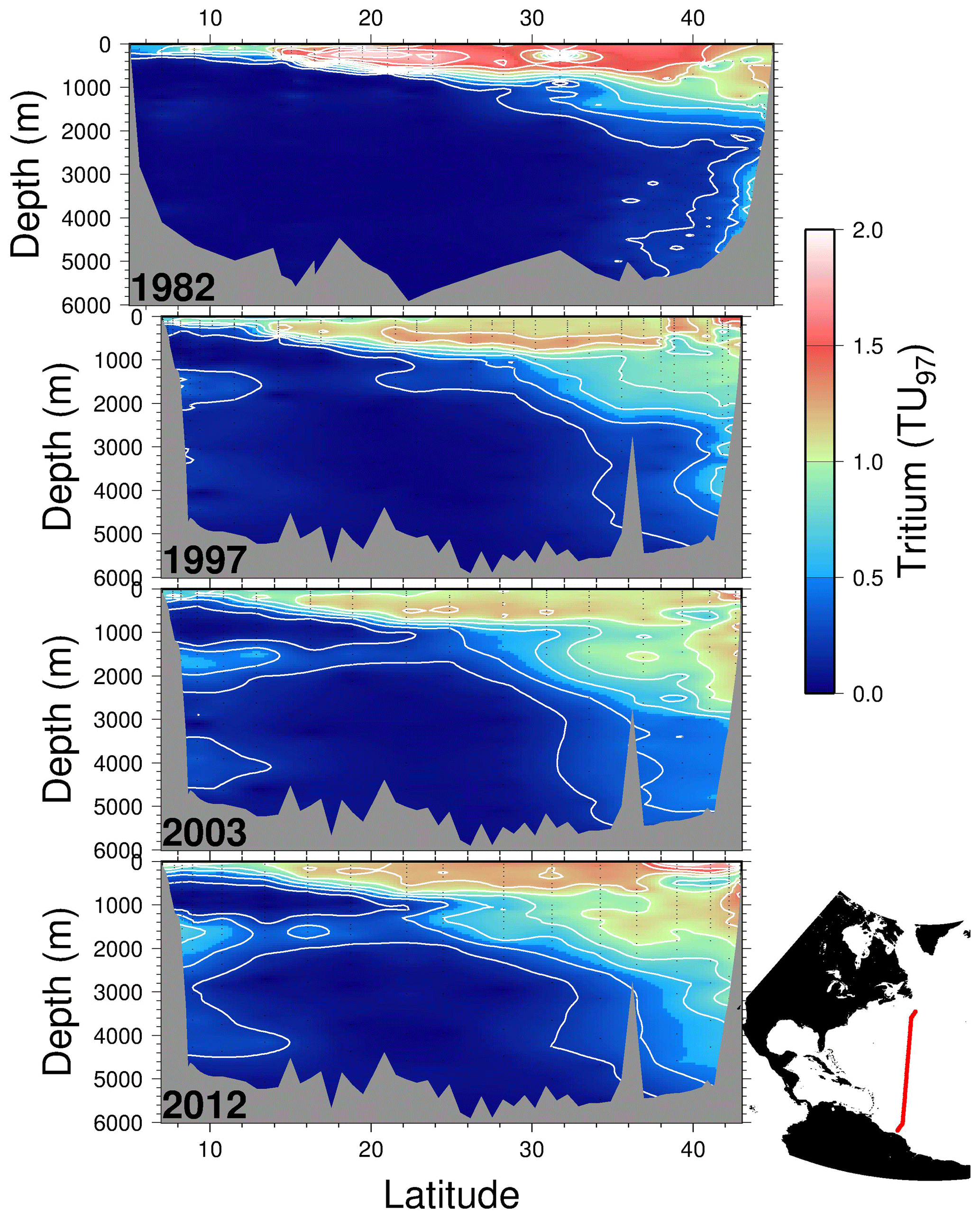
Figure 5 Four meridional tritium sections along roughly 52^∘ W in the North Atlantic taken in 1982, 1997, 2003, and 2012. The tritium concentrations have been decay-corrected to a common time (1 January 1997) for comparison. Contour intervals are 0.2 TU₉₇, and measurement uncertainties are of order 0.01 TU₉₇ or better. Due to differences in cruise tracks, the topography for the 1982 occupation differs from the others.

Equally important is evidence of the southward propagation of the transient tracer along the deep western boundary current system from Nordic and Labrador seas (Doney and Jenkins, 1994). This first appears in 1982 at the northern end of the section between 3000 and 4000 m depth near the bottom of the continental slope. As time progresses, it grows in at intermediate (∼1500 m) and deeper (3500–4000 m) depths at the southern end. This clearly marks the net advective timescales for the deep- and intermediate-depth western boundary currents.

Figure 6 shows the corresponding helium isotope anomaly distribution for the tritium sections. Interpretation of the helium isotope ratio anomaly is a little more complicated than the invasion of bomb tritium, but the buildup of tritiugenic ³He within the main thermocline is an important diagnostic of vertical transport for the subtropical main thermocline. Its retention and back-flux to the ocean surface is a uniquely valuable transient tracer observation, one that parallels the buildup and reflux of inorganic nutrients in the thermocline (e.g., nitrate and phosphate) but in a quantifiably defined manner. Observations of surface water ³He excesses (not shown here) have been used as flux gauges to quantify/constrain regional-scale new production rates (Jenkins, 1988; Jenkins and Doney, 2003; Stanley et al., 2015) as well as upwelling rates (Rhein et al., 2010).

Figure 6 Four meridional δ³He sections along roughly 52^∘ W in the North Atlantic taken in 1982, 1997, 2003, and 2012. Contour intervals are 1 %, and measurement uncertainties are 0.15 %. Due to differences in cruise tracks, the topography for the 1982 occupation differs from the others.

We also include a time series (plotting only the upper 2000 dbar in Fig. 7) for stations within 200 km of Bermuda (32.3^∘ N, 64.7^∘ W) in the subtropical North Atlantic, which highlights some high temporal resolution features in the penetration of tritium into and ingrowth of ³He within the main thermocline and intermediate waters at one location.

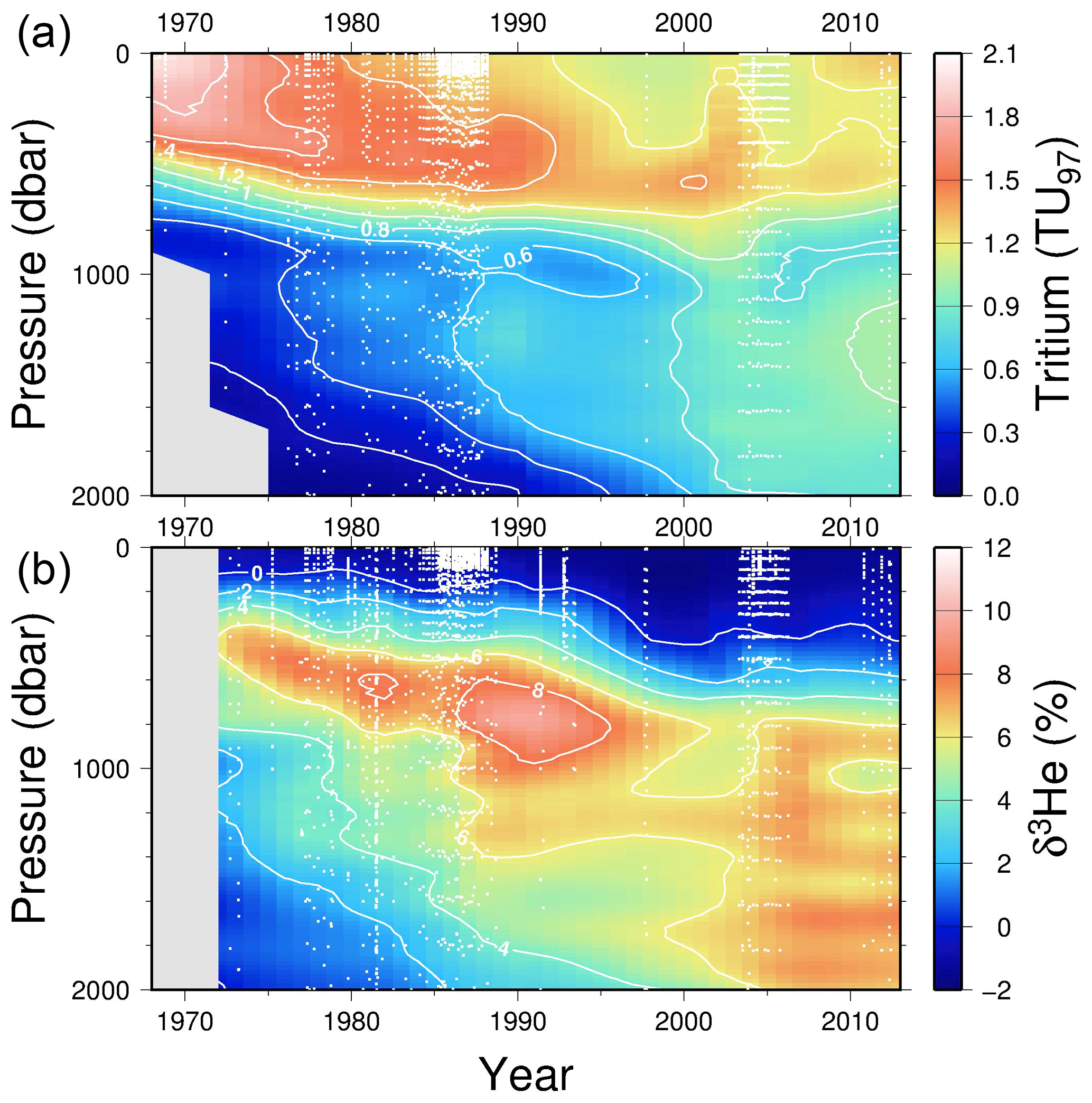
Figure 7 A time series of tritium (upper) and helium isotope measurements in the vicinity of Bermuda (North Atlantic). Tritium values have been decay-corrected to a common time (1 January 1997). White dots indicate sampling depths and times.

Perhaps the most notable features of the oceanic distribution of the helium isotope ratio anomaly are the large tongues emanating from mid-ocean ridges and other volcanic edifices on the sea floor (see the map of the helium isotope ratio anomaly at 2500 m depth in Fig. 8), driven by the roughly order-of-magnitude higher ³He∕⁴He ratio in the earth's mantle compared to the atmosphere (Clarke et al., 1969; Kurz and Jenkins, 1981; Kurz et al., 1982; Lupton and Craig, 1975). It was in fact the initial discovery (Clarke et al., 1969) that sparked continued interest in the oceanic distribution of helium isotopes. In contrast, one sees a different pattern deeper down (4000 m, in Fig. 9), where one sees the relatively ³He-impoverished bottom waters flowing northward into the abyssal Pacific. The ongoing survey of deep helium features on both basin and regional scales continues today, particularly in support of “flux gauge” studies of other trace elements and metals influenced by seafloor hydrothermal processes (e.g., Jenkins et al., 2018a; Resing et al., 2015; Roshan et al., 2016). These are based on recent model-based estimates of the global flux of hydrothermal ³He, which center around 550 mol yr⁻¹ (Bianchi et al., 2010; Holzer et al., 2017; Schlitzer, 2016). This estimate can be usefully compared to the expected global flux of tritiugenic ³He. The global tritium production by atmospheric nuclear weapons tests has been estimated to be of order 3 GCi (Weiss and Roether, 1980, corrected from 1972 to 1963) to 5 GCi (Michel, 1976). Given that the bulk of the tritium “impulse” entered the hydrologic system and subsequently the oceans within a decade or so, one can argue that the production rate of tritiugenic ³He was of order 3000 mol yr⁻¹ in the mid-1970s. By the mid-1990s, this would be of order 1000 mol yr⁻¹. Separating the two “types” of ³He (tritiugenic vs. primordial) in the Northern Hemisphere, where the bulk of the tritium delivery occurred (Doney et al., 1992; Weiss and Roether, 1980), is relatively simple in that the former appears largely at the sea surface, and the latter is concentrated in older, deeper waters. The separation in the Southern Hemisphere is not so simple.

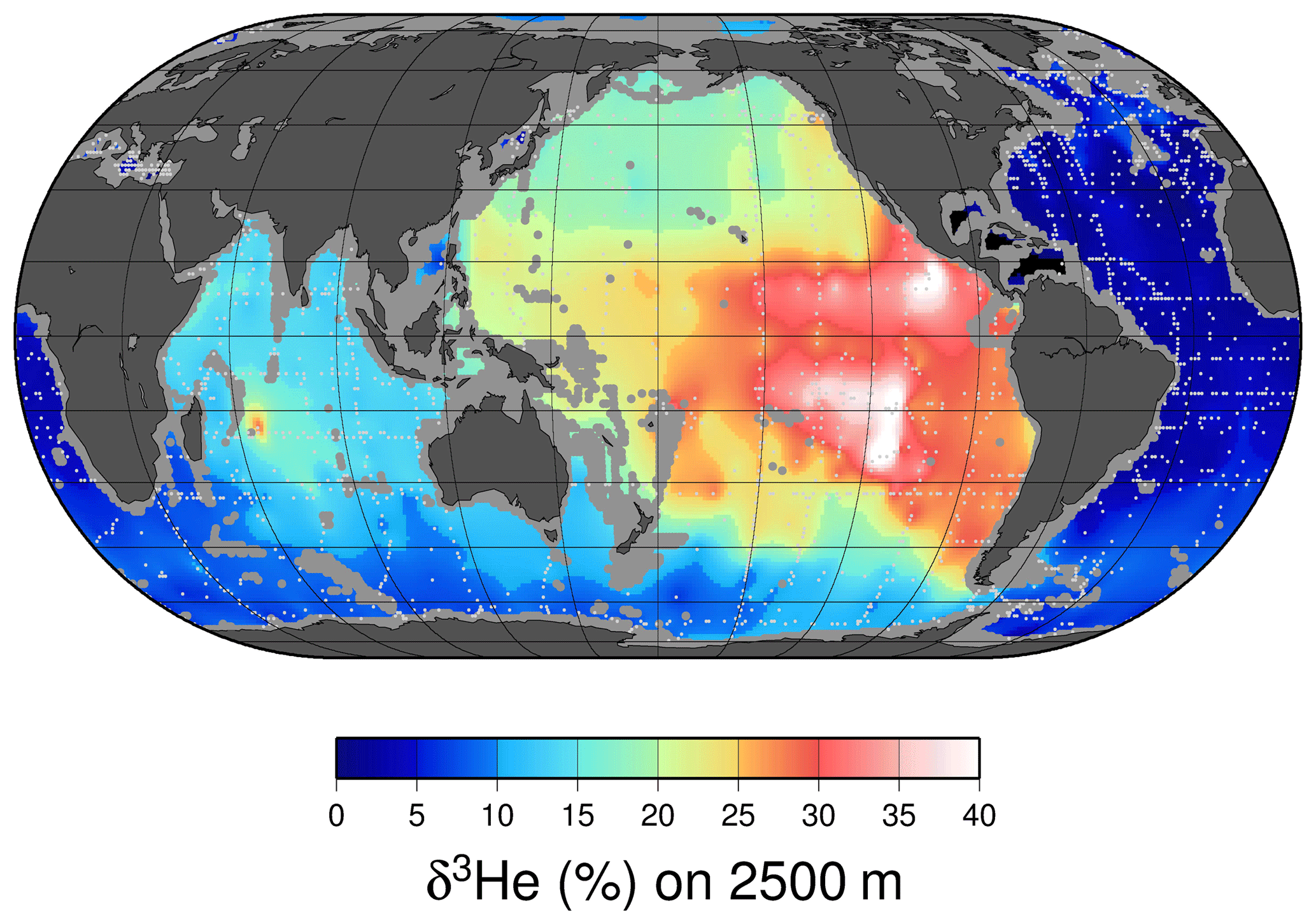
Figure 8 A map of δ³He values at approximately 2500 m depth. The values plotted are simply an average of all measurements within a 1^∘ square between 2250 and 2750 dbar. Depths shallower than 2500 m are masked in gray, and sampling locations are indicated by light gray dots.

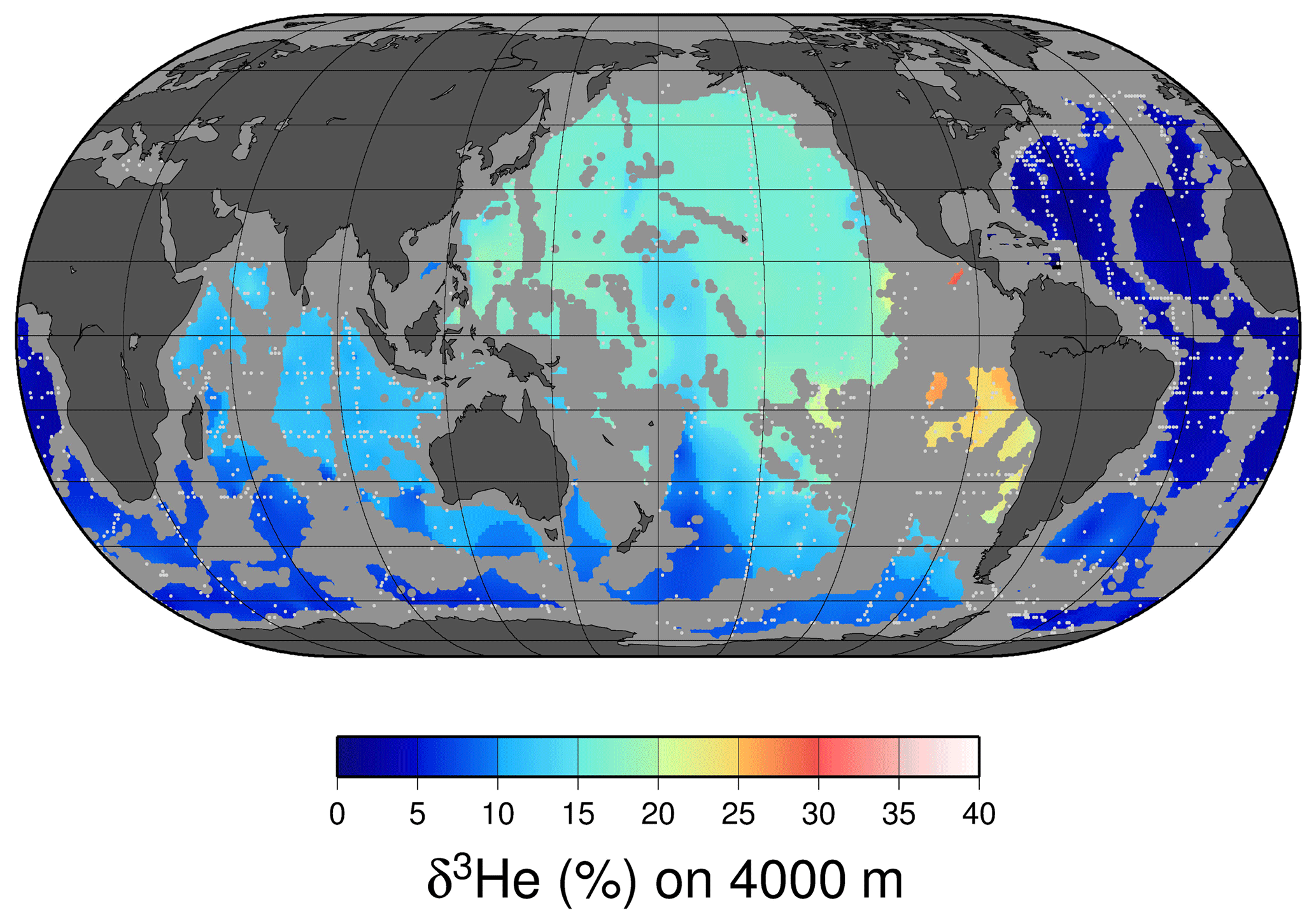
Figure 9 A map of δ³He values at approximately 4000 m depth. The values plotted are simply an average of all measurements within a 1^∘ square between 3750 and 4250 dbar. Depths shallower than 4000 m are masked in gray, and sampling locations are indicated by light gray dots.

4 Data availability

Information about the underlying dataset can be found in Sect. 2.5.

5 Contributors and pioneers

This dataset represents the hard work over many decades of numerous individuals that are not included in the authorship list of this paper. We list their names and affiliations at the time of their contributions in Table 3. The list focuses on those who made the measurements rather than those who may have used the data. We apologize if there are others that we may have missed in this list.

Table 3 Contributing analysts that are not authors on this paper.

We also would like to recognize that the ability to make the measurements presented in this dataset was a consequence of the pioneering work of more than a few inventive and talented individuals. While space does not permit mentioning them all here, we felt it appropriate to highlight a pair of pioneering scientists who conducted landmark studies on ocean tritium and ³He measurements.

5.1 W. Brian Clarke (1937–2002)

Although not the first to measure ³He∕⁴He in the environment (that was done by Aldrich and Nier, 1948), Clarke made the first reported helium isotope measurements in seawater (Clarke et al., 1969). He made his first measurements using a modified single stage magnetic sector, single collector mass spectrometer to a precision of about 2 %. Clarke developed the first compact all-metal branch tube mass spectrometer specifically designed to make ³He∕⁴He measurements ultimately to a precision of 0.1 % to 0.2 %. At the time, conventional wisdom dictated that such measurements (let alone precision measurements) were not possible with a single stage magnetic sector instrument for such high (10⁶) abundance ratios, but Clarke forged ahead anyway. He initially constructed two instruments in the early 1970s, using one at McMaster University in Hamilton, Ontario, Canada, and setting the other machine up at the Scripps Institute of Oceanography in La Jolla, CA, USA, for Harmon Craig and John Lupton. These instruments were used in support of the GEOSECS program and subsequently for a wide variety of other research projects. One of his students (William J. Jenkins) moved to the Woods Hole Oceanographic Institution in Woods Hole, MA, USA, where he extended Clarke's design to construct three other instruments. A post-doctoral investigator from his laboratory (Zafer Top) moved to RSMAS at the University of Miami and constructed a similar machine. Clarke also collaborated with a UK mass spectrometer company to make a commercially produced mass spectrometer available to the global scientific community.

In his early career, Clarke contributed to the study of meteorites and nuclear physics using isotope mass spectrometry. Beginning in 1969 Clarke published a series of ground-breaking papers on ³He∕⁴He measurements in seawater and lakes (Clarke et al., 1969, 1970; Clarke and Kugler, 1973; Craig and Clarke, 1970; Craig et al., 1975; Jenkins and Clarke, 1976; Top and Clarke, 1983; Torgersen and Clarke, 1985). He contributed research to geology, hydrology, limnology, nuclear physics, medicine, and other disciplines and was active until 2002 publishing on ³He-related evidence for and against cold fusion (Clarke, 2001; Clarke and Oliver, 2003; Clarke et al., 2001).

In addition to developing a mass spectrometer capable of measuring ³He∕⁴He ratios to order 0.1 % on sub-nanomolar gas samples, Clarke also created a method to measure environmental levels of tritium (³H) in water samples by the ³He regrowth technique (Clarke et al., 1976), which has become the de facto state of the art in low-level tritium measurements. In addition to being intrinsically simpler than the traditional low-level method (which involved electrolytic enrichment combined with low-level proportional gas counting), this method has proved to be more precise (by more than a factor of 4) and extended the detection limit to lower levels (by as much as an order of magnitude) (Bayer et al., 1989; Jenkins et al., 1983; Lott and Jenkins, 1998).

Clarke was inventive and ingenious in the laboratory with a remarkable ability to recognize opportunities where no one else could and to pursue them to ultimate success. He was an accomplished glass blower and constructed vacuum lines and research apparatuses from scratch using many different kinds of glass (see Fig. 10). Clarke kept unusual work hours when not teaching, generally arriving at the laboratory after lunchtime and toiling into the night. Working with him was a delight due to his good nature and whimsical sense of Irish humor but sometimes challenging because he was an inveterate prankster.

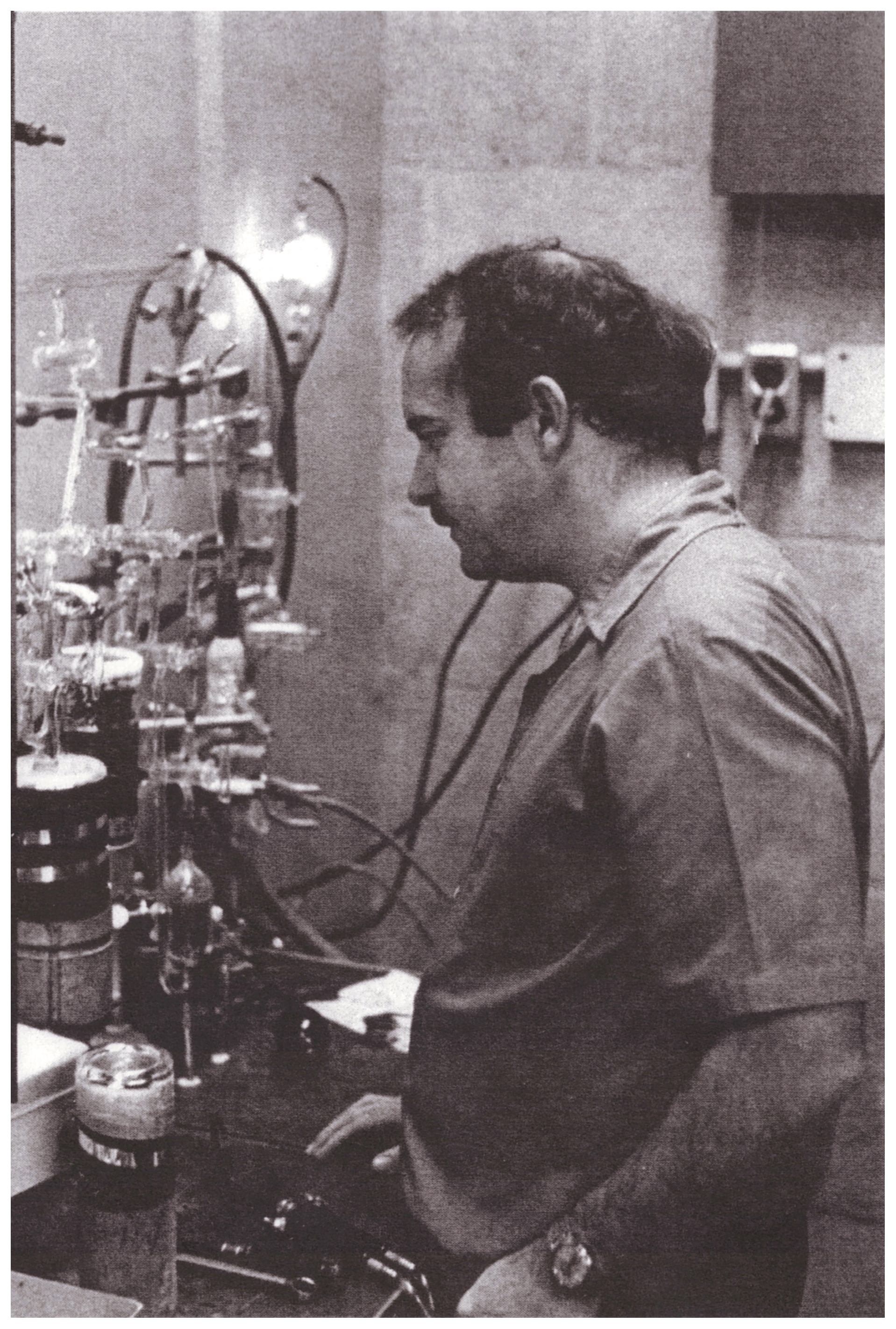
Figure 10 W. Brian Clarke, working on a high vacuum helium extraction apparatus (early 1970s).

5.2 H. Göte Östlund (1923–2016)

Östlund was a pioneer in US ocean tracer measurements, establishing a world-class, low-level counting laboratory dedicated to the measurement of tritium and radiocarbon at the University of Miami. He made distinguished contributions to ocean, atmosphere, and groundwater sciences, in particular to the understanding of the timescales of the transport of fluids through these systems. Östlund had a life-long devotion to the high-quality measurement of radioactive species. He received a BS in chemistry in 1949 and a PhD in chemistry in 1958. Both were from the University of Stockholm. Between 1959 and 1961 Östlund developed the electrolytic enrichment of tritium and deuterium for low-level environmental tritium measurements by gas proportional counting at the Radioactive Dating Laboratory of the Swedish Geological Survey. In the early 1960s, he came to the Rosenstiel School of the University of Miami. At the Rosenstiel School, he built a world-class tritium and radiocarbon counting laboratory that set new standards for low-level counting. His laboratory also processed the samples rapidly, and he generously shared his data with colleagues. As a result, relatively routine collection and analysis of large quantities of samples in a timely manner enabled oceanographers to use the tracer data to gain new insights into the timescales of oceanographic processes. His work paved the way for the acceptance of the next generation of tracer oceanographers, those measuring tritium and helium-3 by mass spectrometry and those measuring the chlorofluorocarbons.

He played a key role in the creation and execution of early global ocean survey programs. He developed electrolytic enrichment techniques for low-level environmental tritium measurements by gas proportional counting (see Fig. 11).

Östlund was a member of the scientific steering committee for the Geochemical Ocean Sections Study (GEOSECS), which was the first global-scale survey of chemical, isotopic, and radiochemical tracers in the ocean (1972–1978). He produced the first large-scale, high-quality mapping of the distribution of tritium in the oceans, which opened oceanographers' eyes to the dynamic and rapid penetration of bomb-produced tracers into the deep ocean.

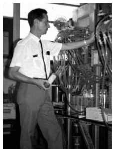
Figure 11 H. Göte Östlund preparing a gas sample for low-level counting analysis (mid-1960s).

Östlund published over 100 papers in peer-reviewed journals on a wide range of subjects. Although his early interests focused on many areas including atmospheric transport, they quickly extended to the hydrologic cycle and the ocean for which he applied radioactive tracers to a spectrum of scientific problems. As a student, he participation in the discovery of the anaesthetic Xylocain. Soon after coming to Miami, he used tritium to show that evaporation from the ocean is the major energy source for hurricanes. To collect samples he even flew into the eye of a hurricane. He and a colleague were the first to use tritium data to show that vertical mixing in the upper layers of the open ocean was an order of magnitude smaller than predicted by mass balance and theory. This was corroborated 20 years later by other investigators using new techniques. A major interest of his was the Arctic Ocean. There he quantified the contributions from ice melt, runoff, and precipitation to the freshwater budget. This budget plays a critical role in the global overturning circulation, which is the leading candidate for modulating decadal to centennial climate.

Östlund was involved in the planning and implementation and served on the scientific steering committees of early global change programs: Geochemical Ocean Sections (GEOSECS), which was the first global-scale survey of chemical, isotopic, and radiochemical tracers in the ocean (1972–1978), followed in the 1980s by Transient Tracers in the Oceans (TTO). The data his laboratory produced and collected under the auspices of these programs have furthered our understanding of the timescales of ocean processes. For example, the data have been used to estimate the flux of anthropogenic carbon dioxide into the ocean, the rate of exchange between the atmosphere and ocean, and rates of deep-water formation. He produced the first large-scale, high-quality mapping of the distribution of tritium in the ocean, which opened a new vista on the dynamic and rapid penetration of bomb-produced tracers into the deep western North Atlantic Ocean. Östlund's leadership as a member and coordinator of the scientific advisory committee for GEOSECS and TTO and his vision and credibility in seeing that an accelerator mass spectrometry facility for ¹⁴C analysis was established in the USA – had a large influence on ocean science. The big oceanographic programs of the past 50 years (GEOSECS through WOCE, CLIVAR, and GO-SHIP) have provided platforms for obtaining large quantities of high-quality tracer data.

Östlund was soft-spoken and gentle in demeanor and generous with his time, advice, and data. He set an example and benchmark for subsequent generations of tracer geochemists for responsibility, honesty, and fairness.