the Creative Commons Attribution 4.0 License.
the Creative Commons Attribution 4.0 License.
 | 22 Feb 2019
A 16-year record (2002–2017) of permafrost, active-layer, and meteorological conditions at the Samoylov Island Arctic permafrost research site, Lena River delta, northern Siberia: an opportunity to validate remote-sensing data and land surface, snow, and permafrost models
Jan Nitzbon
Katharina Anders
Mikhail Grigoriev
Dmitry Bolshiyanov
Moritz Langer
Stephan Lange
Niko Bornemann
Anne Morgenstern
Peter Schreiber
Christian Wille
Sarah Chadburn
Isabelle Gouttevin
Eleanor Burke
Lars Kutzbach
Most of the world's permafrost is located in the Arctic, where its frozen organic carbon content makes it a potentially important influence on the global climate system. The Arctic climate appears to be changing more rapidly than the lower latitudes, but observational data density in the region is low. Permafrost thaw and carbon release into the atmosphere, as well as snow cover changes, are positive feedback mechanisms that have the potential for climate warming. It is therefore particularly important to understand the links between the energy balance, which can vary rapidly over hourly to annual timescales, and permafrost conditions, which changes slowly on decadal to centennial timescales. This requires long-term observational data such as that available from the Samoylov research site in northern Siberia, where meteorological parameters, energy balance, and subsurface observations have been recorded since 1998. This paper presents the temporal data set produced between 2002 and 2017, explaining the instrumentation, calibration, processing, and data quality control. Furthermore, we present a merged data set of the parameters, which were measured from 1998 onwards. Additional data include a high-resolution digital terrain model (DTM) obtained from terrestrial lidar laser scanning. Since the data provide observations of temporally variable parameters that influence energy fluxes between permafrost, active-layer soils, and the atmosphere (such as snow depth and soil moisture content), they are suitable for calibrating and quantifying the dynamics of permafrost as a component in earth system models. The data also include soil properties beneath different microtopographic features (a polygon centre, a rim, a slope, and a trough), yielding much-needed information on landscape heterogeneity for use in land surface modelling.
For the record from 1998 to 2017, the average mean annual air temperature was −12.3 ∘C, with mean monthly temperature of the warmest month (July) recorded as 9.5 ∘C and for the coldest month (February) −32.7 ∘C. The average annual rainfall was 169 mm. The depth of zero annual amplitude is at 20.75 m. At this depth, the temperature has increased from −9.1 ∘C in 2006 to −7.7 ∘C in 2017.
The presented data are freely available through the PANGAEA (https://doi.org/10.1594/PANGAEA.891142) and Zenodo (https://zenodo.org/record/2223709, last access: 6 February 2019) websites.
Please read the corrigendum first before continuing.
-
Notice on corrigendum
The requested paper has a corresponding corrigendum published. Please read the corrigendum first before downloading the article.
-
Article
(19470 KB)
-
The requested paper has a corresponding corrigendum published. Please read the corrigendum first before downloading the article.
- Article
(19470 KB) - Full-text XML
- Corrigendum
- BibTeX
- EndNote


Permafrost, which is defined as ground that remains frozen continuously for 2 years or more, underlies large parts of the land surface in the Northern Hemisphere, amounting to about 15 million km2 (Aalto et al., 2018; Brown et al., 1998; Zhang et al., 2000). The temperature range and the water and ice content of the upper soil layer of seasonally freezing and thawing ground (the active layer) determine the biological and hydrological processes that operate within this layer. Warming of permafrost over the last few decades has been reported from many circum-Arctic boreholes (Biskaborn et al., 2019; Romanovsky et al., 2010). Warming and thawing of permafrost and an overall reduction in the area that it covers have been predicted under future climate change scenarios by the CMIP5 climate models, but at widely varying rates (Koven et al., 2012; McGuire et al., 2018). Continued observations, not only of the thermal state of permafrost but also of the multiple other types of data required to understand the changes to permafrost, are therefore of great importance. The data required include information on conditions at the upper boundary of the soil (specifically on snow cover), on atmospheric conditions, and on various subsurface state variables (such as, e.g. soil volumetric liquid water content and soil temperature). The seasonal snow cover in Arctic permafrost regions can blanket the land surface for many months of the year and has an important effect on the thermal regime of permafrost-affected soils (Langer et al., 2013). The soil's water content determines not only its hydrological and thermal properties, but also the energy exchange (including latent heat conversion or release) and biogeochemical processes.
In view of these dependencies, the data sets presented here, including snow cover and the thermal state of the soil and permafrost, together with meteorological data, will be of great value (i) for evaluating permafrost models or land surface models, (ii) for satellite calibration and validation (cal/val) missions, (iii) in continuing baseline studies for future trend analysis (for example, of the permafrost's thermal state), and (iv) for biological or biogeochemical studies.
The Samoylov research site in the Lena River delta of the Russian Arctic has been investigated by the Alfred Wegener Institute Helmholtz Center for Polar and Marine Research (AWI), in collaboration with Russian and German academic partners, since 1998. The land surface characteristics and basic climate parameter data collected between 1998 and 2011 have been previously published in Boike et al. (2013). Major developments in earth system models, for example through the European PAGE21 project (http://www.page21.org, last access: 6 February 2019), the Permafrost Carbon Network projects (http://www.permafrostcarbon.org, last access: 6 February 2019), satellite calibration and validation missions, and observations through the Global Terrestrial Network on Permafrost (GTN-P) have subsequently led to sustained interest from a broader modelling community in the data obtained.
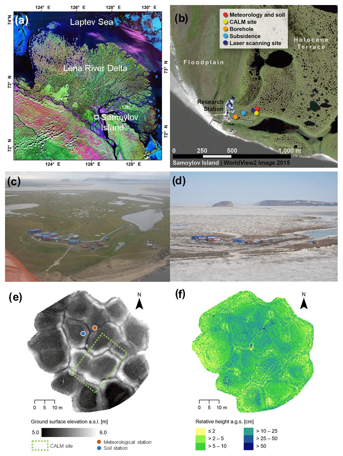
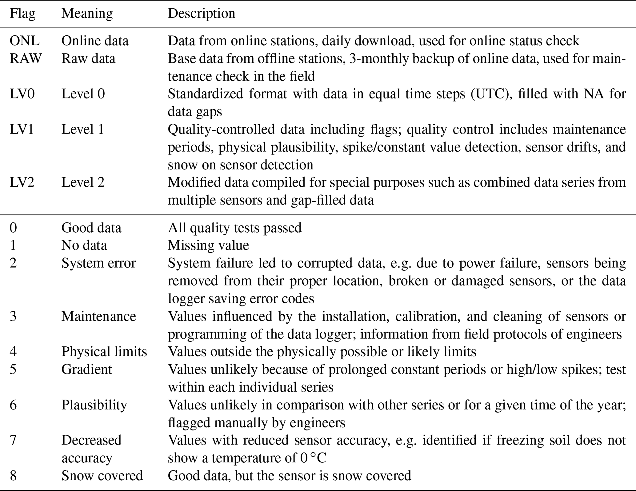
Figure 1Samoylov research site. (a) Location of Samoylov Island in the Lena River delta, northeastern Siberia (Landsat-7 ETM+ GeoCover 2000). (b) Location of instrumentation and measurement sites. (c) The research site under summer conditions (September 2017) and (d) spring conditions (April 2014; photo by Torsten Sachs). (e) Digital terrain model obtained by terrestrial laser scanning (TLS) in September 2017, and (f) relative heights of vegetation derived from TLS data acquired in September 2017. Further details of the methods of TLS data processing are provided in Appendix H.
In this publication we provide information on the research site and full documentation of the data set collected between 2002 and 2017, which can be used for forcing and validation of earth system models (see e.g. Chadburn et al., 2015, 2017; Ekici et al., 2014, 2015). We present data that incorporate subsurface thermal and hydrologic components of heat flux as well as of snow cover properties and meteorological data from the Samoylov research site that are similar to the data published previously for a Spitsbergen permafrost site (Boike et al., 2018a).
The Samoylov research site is located within the continuous permafrost zone on Samoylov Island in the Lena River delta, Siberia (Fig. 1). It has been used for intensive monitoring of soil temperatures and meteorological conditions since 1998 (Boike et al., 2013).
The region is characterized by an Arctic continental climate with low mean annual air temperatures of below −12 ∘C, very cold minimum winter air temperatures (below −45 ∘C), and summer air temperatures that can exceed 25 ∘C, with a thin snow cover and a summer water balance equilibrated between precipitation input and evapotranspiration (Boike et al., 2013).
The study area of the Lena River delta has permafrost to depths of between 400 and 600 m (Grigoriev, 1960). The active-layer thawing period starts at the end of May and the active-layer thickness reaches a maximum at the end of August–beginning of September. Marked warming of this area over the last 200 years has been inferred from temperature reconstruction using deep borehole permafrost temperature measurements in the delta and the broader Laptev Sea region (Kneier et al., 2018).
Samoylov Island is located within a deltaic setting and consists of a flood plain in the western part of the island and a Holocene terrace characterized by ice-wedge polygonal tundra and larger waterbodies in the eastern part (Fig. 1).
The area is generally characterized by ice-rich organic alluvial deposits, with an average ice content in the upper metre of more than 65 % by volume for the Holocene terrace and of about 35 % for the flood plain deposits (Zubrzycki et al., 2013). The Holocene terrace is dominated by ice wedge polygons, so that a considerable volume of the upper soil layer (0–10 m) is characterized by excess ground ice (Kutzbach et al., 2004). Degradation of ice wedges, as observed throughout the Arctic (Liljedahl et al., 2016), occurs at only a few, localized parts of the research site (Kutzbach, 2006). The recent work by Nitzbon et al. (2018) shows that the spatial variability in the types of ice-wedge polygons observed at this study area can be linked to the spatial variability in the hydrological conditions. Furthermore, wetter hydrological conditions have a destabilizing effect on ice wedges and enhance degradation.
The total mapped area of the polygonal tundra on Samoylov Island (excluding the floodplain) is composed of 58 % dry tundra, 17 % wet tundra, and 25 % water surfaces, of which 10 % is overgrown water and 15 % is open water (Muster et al., 2012, Fig. 3a). The landscape is characterized by polygonal tundra, i.e. a complex mosaic of low- and high-centred polygons (with moist to dry polygonal ridges and wet depressed centres) and larger waterbodies (Muster, 2013; Muster et al., 2012). The polygonal tundra microtopography, polygon rims, slopes, and depressed centres are clearly distinguishable. Depressed polygon centres are typically water saturated or have water levels above the ground surface (shallow ponds). High-centred polygons have inverse microtopography, i.e. drier elevated centres and wet surrounding troughs. Polygonal ponds and troughs make up about 35 % of the total water surface area on the island (Boike et al., 2013).
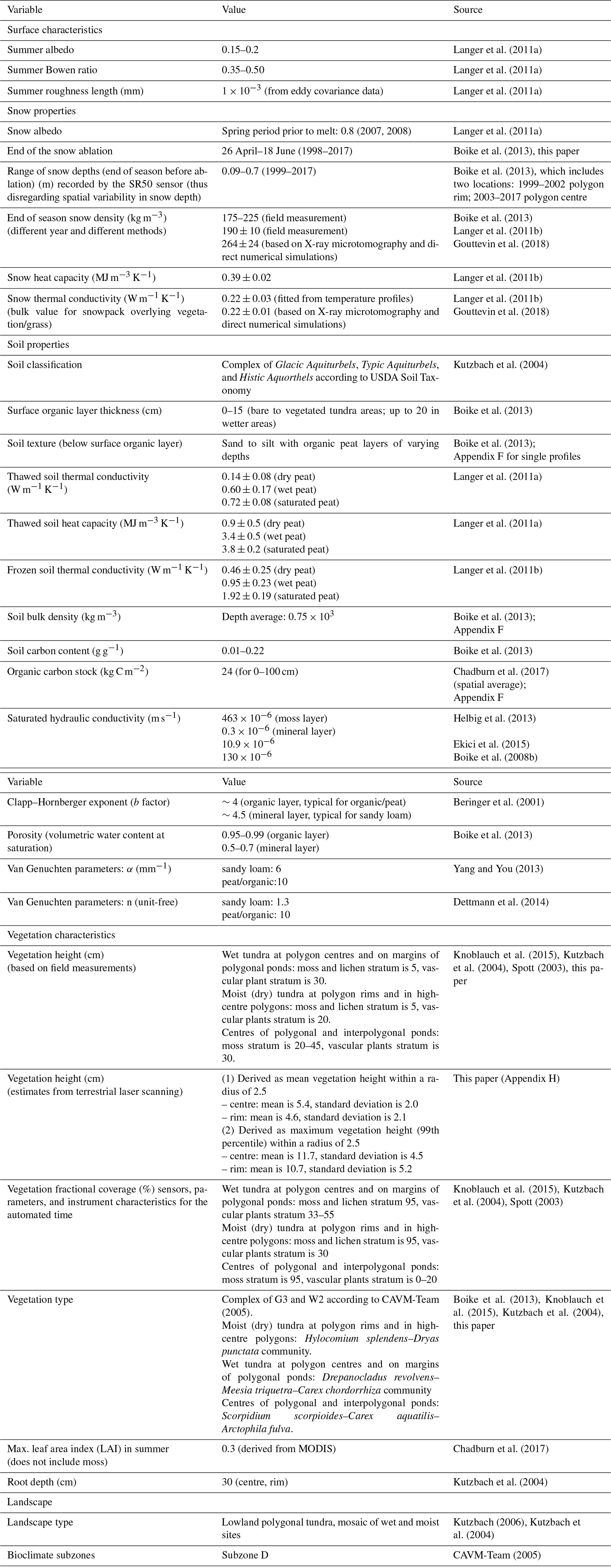
Previous research based at the research site has focused on greenhouse gas cycling (Abnizova et al., 2012; Knoblauch et al., 2018, 2015; Kutzbach et al., 2004, 2007; Langer et al., 2015; Runkle et al., 2013; Sachs et al., 2010, 2008; Wille et al., 2008; Holl et al., 2019), aquatic biology (Abramova et al., 2017), upscaling of land surface characteristics and parameters from ground-based data to remote-sensing data (Cresto Aleina et al., 2013; Muster et al., 2013, 2012), and hydrology (Boike et al., 2008b; Fedorova et al., 2015; Helbig et al., 2013). Data from a few years have also been used in earth system modelling (Chadburn et al., 2015, 2017; Ekici et al., 2014, 2015) and for modelling land surface, snow, and permafrost processes (Gouttevin et al., 2018; Langer et al., 2016; Westermann et al., 2016, 2017; Yi et al., 2014; Aas et al., 2019). Table 1 summarizes the characteristics of the research site, based on data in previous publications and additional data included in this paper.
Table 1Site description parameters for earth system model input. Values have been computed and compiled for the Samoylov research site and surrounding areas.
This paper presents, for the first time, a complete data archive and descriptions in the form of the following data sets: (i) a full range of meteorological, soil thermal, and hydrologic data from the research site covering the period between 2002 and 2017 (Fig. 2), (ii) high spatial resolution data from terrestrial laser scanning of the research site completed in 2017, with resulting data sets for a digital terrain model and for vegetation height, (iii) time-lapse camera images, and (iv) a data set containing specially compiled or processed data sets for those parameters that were measured in the period from 1998 to 2002, thus extending the record to form a long-term data set, as initiated in Boike et al. (2013). The processing and level structure is described in detail in Sect. 4. Additional data such as soil properties and soil carbon content are also included in this paper in order to provide a complete set of data and parameters suitable for earth system, conceptual, and land surface modelling. All of these data are archived in the PANGAEA data libraries (Boike et al., 2018b, c, d) and the measuring principles and analysis are described in this paper.
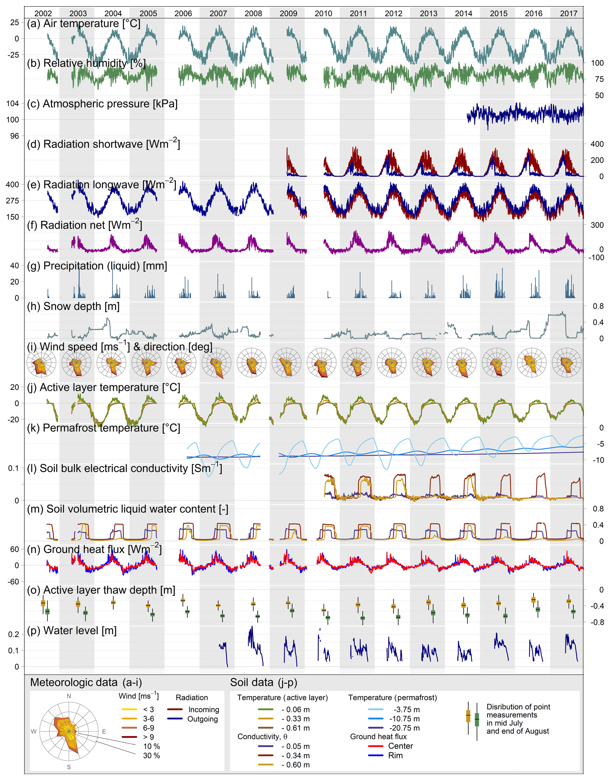
Figure 2Time series (daily mean values) of Samoylov data presented in this paper: (a–i) meteorological data and (j–p) soil data. Seasonal average active-layer thaw depth (o) was measured at the 150 data points on the Samoylov CALM grid. Further details on the sensors and periods of operation are given in Table 2.
Data logging between 2002 and 2013 at the research site was powered by a solar panel and a wind turbine generator, and the data were retrieved manually during site visits once or twice a year, when visual inspections were also made of the sensors. Data gaps prior to 2013 resulted mainly from problems with the site's energy supply, such as problems with the solar or wind charge controller. No other gap filling has been undertaken, but previous publications (e.g. Langer et al., 2013) suggest that reanalysis data, such as ERA-Interim, could be used for this purpose. In Chadburn et al. (2017), a method for correcting reanalysis data to better represent the site is described and applied. The gap-free meteorological data set that was produced and used in Chadburn et al. (2017) is now available on the PANGAEA database (Burke et al., 2018), making it easy for modellers to begin running the Samoylov site and therefore to make good use of our data.

Figure 3Mean annual, maximum, and minimum permafrost temperatures at different depths between 2006 and 2017, as recorded in the Samoylov Island borehole. Mean annual temperatures are based on the period 1 September 2006 to 31 August 2007 and 1 September 2016 to 31 August 2017. Maximum and minimum annual variations are based on the same time period and computed from mean daily temperatures. The upper 3.5 m below the surface is shaded in grey since we recommend not using these data for active-layer thermal processes.
Since 2013 the research site has been connected to the main electricity supply of the new Russian research station, resulting in a much improved data collection with almost no data gaps.
Details of the sensors used are provided in the following sections, as well as descriptions of the data quality and cleaning routine (Sect. 4). The instruments can be divided into aboveground sensors (meteorological) and below-ground sensors (e.g. soil sensors). Further detailed information on the sensors can be found in Table 2, which summarizes all of the instruments and relevant parameters, as well as in the appendices B to H (metadata, description of instruments, and calculations of final parameters). Figure 2 presents a time series of selected parameters measured between 2002 and 2017.
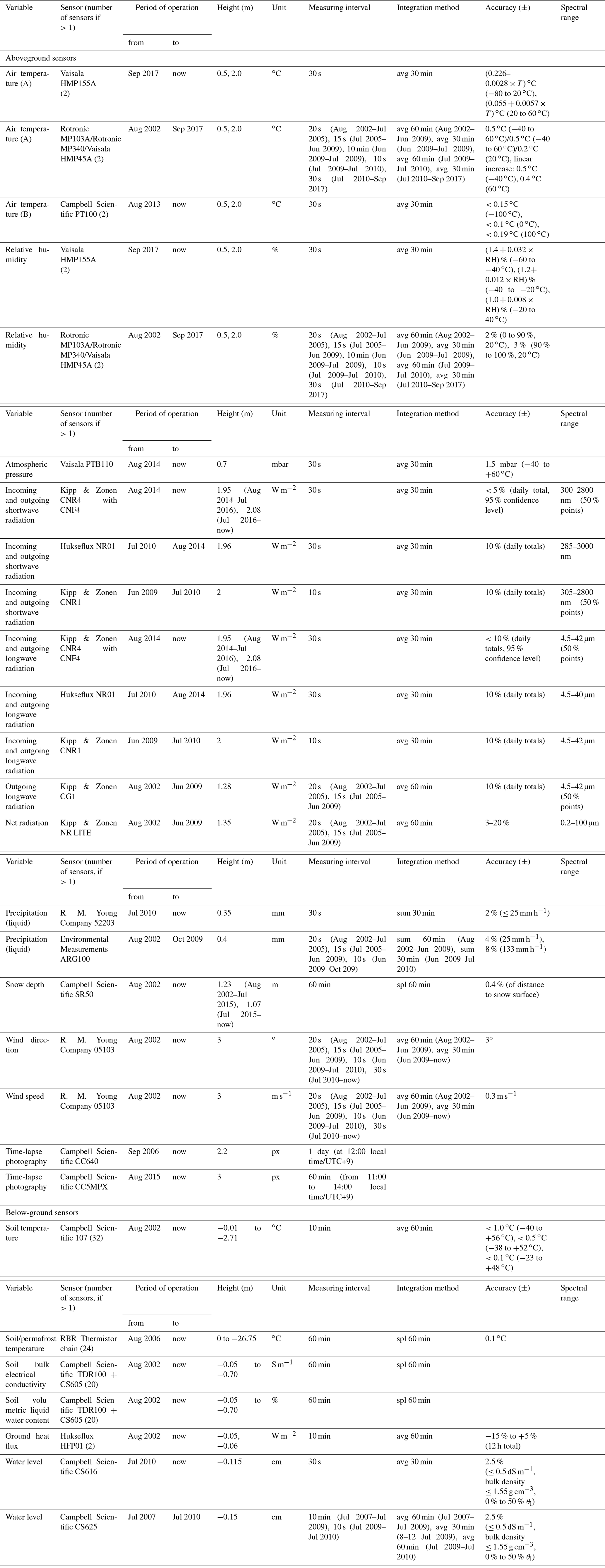
Table 2List of sensors, parameters, and instrument characteristics for the automated time series data from the Samoylov research site, 2002–2017. Positive heights are above the ground surface; negative heights are below the ground surface. Sensor names refer to the original manufacturer brand name (e.g. the Vaisala PTB110 air pressure sensor is distributed by Campbell Scientific as model CS106). Integration methods are average (avg), sample (spl), and sum.
3.1 Meteorological station data
The standard meteorological variables described in this section were averaged over various intervals (Table 2) with the averages, sums, and individual values all being saved hourly until 2009 and half-hourly thereafter. The sampling intervals changed as a result of different logger and sensor setups and different available power sources. Sensors were connected directly to data loggers. A number of different data logger models from Campbell Scientific were used over the years (CR10X between 2002 and 2009, CR200 between 2007 and 2010, and CR1000 since 2009), together with an AM16/32A multiplexer.
Table 3Description of data level and quality control for data flags. Most data are flagged automatically; some are occasionally flagged manually (Flag 3: maintenance, Flag 6: plausibility). Online data transfer is not currently operational but is planned for the future.
3.1.1 Air temperature, relative humidity
Air temperature and relative humidity were measured at 0.5 and 2 m above the ground (starting with hourly averages at 2.0 m until 30 June 2009 and at 0.5 m until 26 July 2010, with half-hourly averages thereafter) using Rotronic and Vaisala air temperature and relative humidity probes protected by unventilated shields (Fig. B1 and Table 2). According to the sensor's manuals, the HMP45 sensors have a measurement limit of −39.2 ∘C, but we recorded data down to −39.8 ∘C. During extreme cold-air temperature periods, for example between 1 February and 15 March, 2013, constant air temperature values were recorded at the sensor's output limit. These data periods were manually flagged (Flag 6: consistency; Table 3) using a lower temperature limit of −39.5 ∘C.
Also of importance is the decrease in accuracy of the air temperature and humidity data with decreasing temperature and moisture content. For example, the accuracy for the HMP45A sensor at 20 ∘C is ±0.2 ∘C, but at −40 ∘C it is ±0.5 ∘C. Campbell Scientific PT100 temperature sensors were installed on 22 August 2013 alongside the temperature and humidity probes, at the same heights but in separate unventilated shields, in order to circumvent this problem. Since 17 September 2017 Vaisala HMP155A air temperature and relative humidity probes were installed, which enable the full range of temperatures (below −40 ∘C). The uncertainty in all the temperature measurements ranges between 0.03 and 0.5 ∘C, depending on the sensors used; the uncertainty in the relative humidity measurements ranges between 2 % and 3 %. The measurement heights were not adjusted with respect to the snow surface during periods of snow cover accumulation or ablation. The lower probes (at 0.5 m) were only completely snow covered during 2 months of the 2017 winter season (16 April–11 June 2017), as observed in photographic images, and therefore this time period is flagged in the data series (Flag 8: snow covered; Table 3).
3.1.2 Wind speed and direction
The wind speed and direction were measured using a propeller anemometer (R. M. Young Company 05103, Fig. B2), which was calibrated towards geographic north. This was done by orienting the centre line of the sensor towards true north (using a GPS reference point) and then rotating the sensor base until the data logger indicated 0∘. The averaged wind direction, its standard deviation, and the wind speed were all recorded at hourly intervals until 30 June 2009 and at half-hourly intervals thereafter. Since August 2015, wind maximum and minimum wind speed are also recorded. The mean wind speeds and directions were calculated using every value recorded during the measurement interval. The standard deviation of the wind direction was calculated using the algorithm provided by the Campbell Scientific data logger.
3.1.3 Radiation
The net radiation was measured between 2002 and 2009 using a Kipp & Zonen NR Lite net radiometer; outgoing longwave radiation was also measured using a Kipp & Zonen CG1 pyrgeometer. Since 2009, various four-component radiometers were used (Table 2). The averaged values were stored at hourly intervals until 30 June 2009 and at half-hourly intervals thereafter. Further details of the measuring periods and the specifications for the different sensors can be found in Table 2. Although all radiation sensors were checked for condensation, dirt, physical damage, hoar frost, and snow coverage during the regular site visits, the instruments were largely unattended and their accuracy is therefore estimated to have been ±10 %. Our quality analysis also includes flagging the data during those periods in which shortwave incoming radiation was lower than shortwave outgoing radiation by 10 W m−2 using Flag 6 (plausibility, values unlikely in comparison with other sensor series or for a given time of the year). Between 30 June 2009 and 21 July 2017, less than 1 % of the data were flagged. Since August 2014 a Kipp & Zonen CNR4 four-component radiation sensor is operative, together with a CNF4 ventilation unit to prevent condensation (Fig. B3). The additional heating available for the CNR4 sensor was never used.
3.1.4 Rainfall
Unheated and unshielded tipping bucket rain gauges (Environmental Measurements ARG100 and R. M. Young Company model 52203) were installed directly on the ground on 31 August 2002 (ARG100) and 26 July 2010 (52203). The Environmental Measurements ARG100 liquid precipitation probe was damaged during the winter of 2009–2010. By installing the gauge close to the ground, the risk of wind-induced tipping of the bucket, which would lead to false data records, can be reduced (as observed by Boike et al., 2018a). Due to the typically low snow heights, the risk of snow coverage of the instrument is also very low.
The instruments measure only liquid precipitation (rainfall) and not winter snowfall. The tipping buckets were checked regularly during every summer by pouring a known volume of water into the bucket and carrying out frequent visual inspections for dirt or snow during each site visit. These calibration data are flagged with Flag 3 (maintenance periods).
3.1.5 Snow depth
The snow depth around the station has been continuously monitored since 2002 using a Campbell Scientific SR50 sonic ranging sensor (Fig. B4). The sensor measures the distance between the sensor and an object or surface, which could be the upper surface of the snow (in winter) or the water surface, ground surface, or vegetation (in summer). On 17 July 2015 a metal plate was placed directly beneath the ultrasonic beam to reduce the amount of noise in the reflected signal due to surface vegetation (Fig. B4). The acoustic distance data obtained from the sonic sensor were temperature-corrected using the formula provided by the manufacturer (Appendix C) using the air temperature measured at the Samoylov meteorological station.
To obtain the snow depth, the distance of the sensor from the surface was recorded over the summer and the mean was calculated. The recorded (corrected) winter distances are then subtracted from this mean (previous) summer value to obtain snow depth. Due to seasonal thawing, the ground surface can subside by a few centimetres over the summer season (and therefore no longer be set to zero), resulting in negative heights for the ground-surface level being computed. In contrast, vegetation growth and higher water levels (e.g. as observed in 2017) will result in positive heights. The distance measurements collected during the snow-free season are not removed from the series or corrected, since they provide potentially useful information about these processes.
The SR50 sensor acquires data over a discoidal surface with a radius that ranges from 0.23 m (0.17 m2) in snow-free conditions to 0.19 m (0.12 m2) with 20 cm of snow. This footprint disk is located in the centre of a low-centred polygon for which the spatial variability of snow has been investigated by Gouttevin et al. (2018). The microtopography of this polygonal tundra (characterized by rims, slopes and polygon centres) was identified as a profound driver of spatial variability in snow depth: at maximum accumulation in 2013 rims typically had 50 % less snow cover and slopes 40 % more snow cover than polygon centres. However, the snow cover within each topographical unit also exhibited spatial variability on a decimetre scale (Gouttevin et al., 2018), probably resulting from underlying micro-relief (notably vegetation tussocks) and processes such as wind erosion. This variability can affect the representativity of the SR50-measured snow depth data and visual data obtained from time-lapse photography can therefore be extremely important (see next section).
3.1.6 Time-lapse photography of snow cover and land surface
In order to monitor the timing and pattern of snow melt an automated camera system (Campbell Scientific CC640) was set up in September 2006 to photograph the land surface in the area in which the instruments were located (Figs. B5 to B7). The images are used as a secondary check on the snow cover figures obtained from the depth sensor and are also valuable for monitoring the spatial variability of snow cover across polygon microtopography. During the polar night the image quality was found to be somewhat reduced and a second camera with a better resolution (Campbell Scientific CC5MPX) was therefore installed in August 2015 to record high-quality images in low-light conditions over the winter period.
3.1.7 Atmospheric pressure
A Vaisala PTB110 sensor in a vented box was installed next to the data loggers at the meteorological station (Fig. B1) in August 2014 to measure atmospheric pressure.
3.1.8 Water levels
The suprapermafrost ground-water level, i.e. water level of the seasonally thawed active layer above the permafrost table within one polygon, was estimated using Campbell Scientific CS616 and CS625 water content reflectometer probes installed vertically in the soil and air, with the sensor's ends standing upright (Appendix D). The advantage of this method is that the sensor can remain in the soil during freezing and subzero temperatures, whereas pressure transducers need to be removed over winter and then reinstalled. For the unfrozen periods, the soil was measured by a dielectric device is a mixture of air, water, and soil particles. The sensor outputs a signal period measurement from which the bulk dielectric number is usually calculated. The dielectric number (also referred to as the relative permittivity or dielectric constant) is then used to calculate the volumetric water content using an empirical polynomial calibration provided by the manufacturer. We use the signal period output of the CS616 and CS625 water content reflectometer probes (Campbell Scientific, 2016) and a site-specific calibration and convert these values to water level with respect to the sensor base (Appendix D).
3.2 Subsurface data on permafrost and the active layer
3.2.1 Instrument installation at the soil station and soil sampling
In order to take into account any possible effects of heterogeneity in vegetation and microtopography at the research site (e.g. due to the presence of polygons), instruments for measuring the soil's thermal and hydrologic dynamics (Table 2) were installed at a number of different positions within a low-centred polygon.
Instrument installation and soil sampling in 2002
A new measurement station was established in August 2002, with instruments installed in four profiles (Appendices B2 and F). Four pits were dug through the active layer and into the permafrost (Figs. B8 and B9), one at the peak of the elevated polygon rim (BS-1), one on the slope (BS-2), a third in the depressed centre (BS-3), and one above the ice wedge (Wille et al., 2003).
The surface was carefully cut and the excavated soil stockpiled separately according to depth and soil horizon in order to be able to restore the original profile following instrument installation. The soil material is generally stratified fluviatile (and aeolian) sands and loams, with layers of peat. The BS-1 and BS-2 soil profiles are classified as Typic Aquiturbels, while the BS-3 soil profile is classified as Typic Historthel, according to US Soil Taxonomy (Soil Survey Staff, 2010). The thaw depth was between 17 and 40 cm thick at the time of instrument installation.
Sensors were installed to cover the entire depth range of the profile, i.e. from the very top, through the active layer and into the permafrost soil. The sensors were positioned according to the soil horizons so that every horizon in the profile contained at least one probe.
Sensors were installed horizontally into the undisturbed soil profile face beneath different microtopographical features and the pits were then backfilled (Figs. B10 and B13).
Soil samples were collected before instrument installation so that physical parameters could be analyzed. Soil properties within the soil profiles, including the soil organic carbon (OC) content, nitrogen (N) content, soil textures, bulk densities, and porosities can be found in Appendix F.
The Typic Aquiturbels from the peak and the slope of the polygon rim show cryoturbation features due to the formation of thermal contraction polygons. The Typic Historthel in the polygon centre, on the other hand, does not have any cryoturbation features and is characterized by peat accumulation under waterlogged conditions. (Fig. F1).
3.2.2 Soil temperature
Soil temperature sensors were installed over vertical 1-D profiles in 2002 beneath a polygon centre, slope, and rim. A measurement chain of temperature sensors was also installed in the ice wedge down to a depth of 220 cm. Their positions are shown in Fig. B13. The temperatures were initially measured using Campbell Scientific 107 thermistors connected to a Campbell Scientific CR10X data logger with a Campbell Scientific AM416 multiplexer. Campbell Scientific's worst-case example, with all errors considered to be additive, is given as ±0.3 ∘C between −25 and 50 ∘C. The average deviation from 0 ∘C determined through ice bath calibration prior to installation was 0.008 ∘C (maximum: 1.0 ∘C; minimum: −0.56 ∘C, standard deviation: 0.33 ∘C). The sensors cannot be recalibrated once they have been installed. Phase change temperatures during spring thaw and fall refreezing are stable (the zero-curtain effect in freezing and thawing soils of periglacial regions). Assuming that freezing point depression (due to the soil type and soil water composition) does not change significantly from year to year, these periods can be used to evaluate sensor stability. Between 2002 and 2009 the data logger and multiplexer were not replaced, which resulted in a reduced accuracy of up to ±0.7 ∘C during the winter freeze-back periods in 2009 for two of the sensors near to the surface (centre of the polygon at −1 cm, rim of the polygon at −2 cm below the ground surface, respectively). The zero-curtain period during fall–winter, where temperatures in the ground are stabilized at 0 ∘C during phase change, offers an accuracy test for sensors that cannot be retrieved. For the remaining sensors the accuracy was better, up to ±0.5 ∘C. The affected data are flagged in the data series (Flag 7: decreased accuracy; Table 3). The data quality improved greatly following the installation of a new data logger and multiplexer system (Campbell Scientific CR1000 data logger, AM16/32A multiplexer) in 2010 and the maximum offset at 0 ∘C during freeze-back was ±0.3 ∘C.
3.2.3 Soil dielectric number, volumetric liquid water content, and bulk electrical conductivity
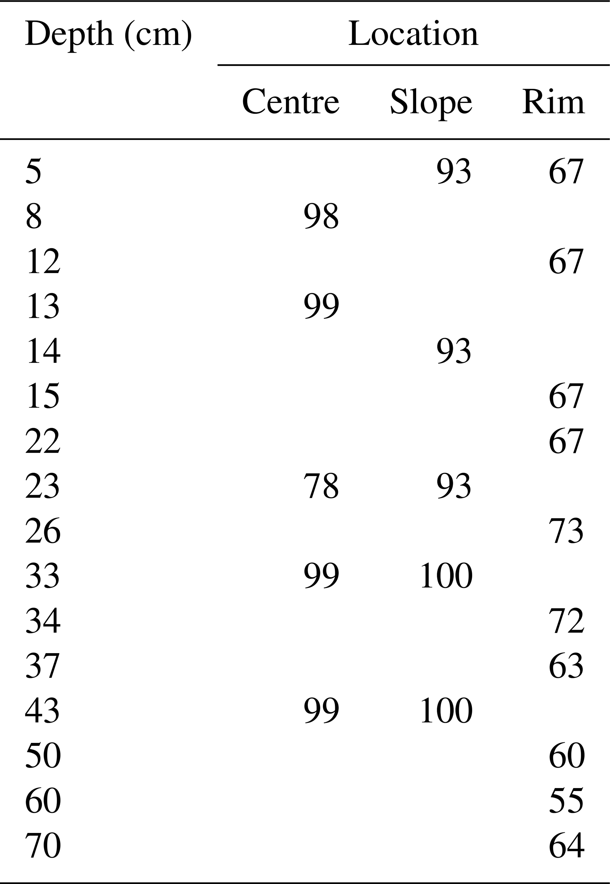
Time-domain reflectometry (TDR) probes were installed horizontally in three soil profiles adjacent to the temperature probes. The fourth profile in the ice wedge only records temperature data (see Sect. 3.2.2., Figs. B11 and B13). The TDR probes automatically record hourly measurements of bulk electrical conductivity (from 25 July 2010 only), and the dielectric number, obtained by measuring the amplitude of the electromagnetic wave over very long time periods and the ratio of apparent probe length to real probe length (the La∕L ratio), corresponding to the square root of the dielectric number. A Campbell Scientific TDR100 reflectometer was used together with an SDMX50 coaxial multiplexer, custom-made 20 cm TDR probes (Campbell Scientific CS605) connected to a Campbell Scientific CR10X data logger between 2002 and 2010 and to a Campbell Scientific CR1000 data logger thereafter. All TDR probes were checked for offsets following the method described in Heimovaara and de Water (1993) and in Campbell Scientific's TDR100 manual (Campbell Scientific, 2015). The calibration delivered a probe offset of 0.085 (an apparent length value used to correct for the portion of the probe rods that is covered with epoxy), which was used instead of the value of 0.09 suggested by Campbell Scientific. The dielectric number ε (dimensionless) and the computed volumetric liquid water values θl (volume/volume) in frozen and unfrozen soil are provided as part of the time series data set. The calculation for volumetric liquid water content takes into account four phases of the soil medium (air, water, ice, and mineral) and uses the mixing model from Roth et al. (1990) (Appendix C).
The data are generally continuous and of high quality, and the absolute accuracy is estimated to be better than 5 %. This is estimated from the maximum deviation of calculated volumetric liquid water content below and above the physical limits (between 0 % and 1 % or 0 % and 100 %). A probe located at 0.37 m depth beneath the polygon rim showed a shift of about 3 % (up and down) in the volumetric liquid water content during the summers of 2009, 2013, and 2014, for which we could not find any technical explanation. This shift is flagged in the data series (Flag 6: consistency; Table 3).
Time-domain reflectometry was also used to measure the bulk soil impedance, which is related to the soil's bulk electrical conductivity (BEC). These data were used to infer the electrical conductivity of soil water and solute transport over a 12-month period in the active layer of a permafrost soil (Boike et al., 2008a). The impedance can be determined from the attenuation of the electromagnetic wave travelling along the TDR probe after all multiple reflections have ceased and the signal has stabilized. The bulk conductivities were recorded hourly using the TDR setup described above in this section. Because no calibration was done, and the TDR probes were custom made to 20 cm, a probe constant (Kp) of 1 was used for BEC waveform retrieval; Campbell Scientific suggests a Kp for the CS605 probes of 1.74. Measurements of electrical conductivity and the dielectric number were affected by irregular spikes and possibly also by a sensor drift similar to that in the soil temperature measurements and thus flagged until August 2015 (Flag 6). Data quality improved significantly after August 2015 when the Campbell Scientific coaxial SDMX50 multiplexers were exchanged for SDM8X50 and the electrical grounding system was improved. The dielectric numbers, computed volumetric liquid water contents, and soil bulk electrical conductivities can be found in the time series data set.
3.2.4 Ground heat flux
Two Hukseflux HFP01 heat flux plates were installed on 24 August 2002 and recorded ground heat flux at 0.06 (rim) and 0.11 m (centre) depth since then (Fig. B12). The manufacturer's calibration values were used to record heat flux in W m−2 (Hukseflux, 2016). Downward fluxes are positive and occur during spring and summer, while upward heat fluxes are negative and typically occur during fall and winter.
3.2.5 Permafrost temperature
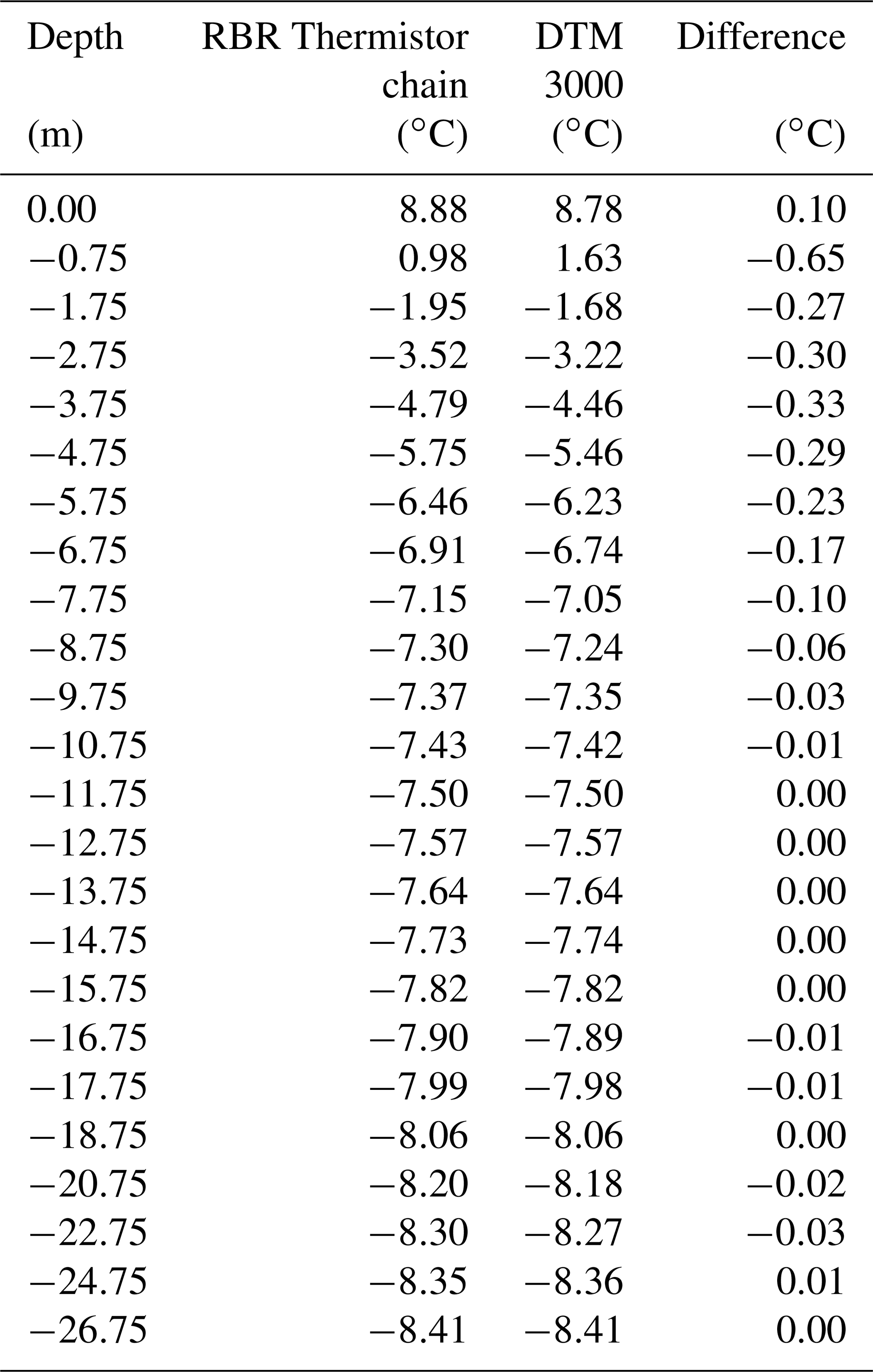
The monitoring of essential climate variables (ECVs) for permafrost has been delegated to the Global Terrestrial Network on Permafrost (GTN-P), which was developed in the 1990s by the International Permafrost Association under the World Meteorological Organization. The GTN-P has established permafrost temperature and active-layer thickness as ECVs in (1) the TSP (Thermal State of Permafrost) data set and (2) the CALM (Circumpolar Active Layer Monitoring) monitoring programme (Romanovsky et al., 2010; Shiklomanov et al., 2012). A 27 m deep borehole was drilled in March 2006 with the objective to establish permafrost temperature monitoring (Fig. 1, Appendix E). A 4 m long metal pipe (diameter 13 cm; extending 0.5 m above and 3.5 m below the surface) was used for stability and to prevent the inflow of water during summer season when the upper ground is thawed. In August 2006, 24 thermistors (RBR thermistor chain with an RBR XR-420 logger) were installed, one at the ground surface and 23 between 0.75 and 26.75 m depth, inside a PVC tube (Fig. E2). A second PVC tube was inserted into the borehole and the remaining air space in the borehole was backfilled with dry sand. Temperatures were recorded at hourly intervals, with no averaging; no data were recorded between September 2008 and April 2009. We recommend that the temperature data from the sensors at the ground surface, at 0.75, 1.75 and 2.75 m depths should not be used due to the possibility of it having been affected by the metal access pipe. The data from these sensors have not been flagged as they are of high quality, but they may not provide an accurate reflection of the actual temperatures. They show above-zero temperatures down to 1.75 m during summer in contrast to the active-layer soil temperatures (Fig. 2). In contrast, the CALM active-layer thaw never exceeded > 0.8 m since 2002 at all grid locations.
The second PVC tube was used for comparison measurements at the same depths in the borehole. The differences between the calibrated reference thermometer (PT100) showed values between ±0.03 and ±0.33 ∘C (Appendix E, Table E1).
The data record shows that depth of zero annual amplitude (ZAA, where seasonal temperature changes are negligible, ≤0.1 ∘C) is located below 20.75 m. At 26.75 m, temperatures fluctuate with a maximum of 0.05 ∘C. The annual mean temperatures between the start and end of the time series, as well as minimum and maximum temperatures, are displayed in Fig. 3 (trumpet curve). The permafrost warms at all depths within this 10-year period, but is most pronounced at the surface. At 2.75 m, the mean annual temperature increased by 5.7 ∘C (from −9.2 to −3.5 ∘C), at 10.75 m by 2.8 ∘C (from −9.0 to −6.2 ∘C), and at ZAA of 20.75 m by 1.3 ∘C (from −9.1 to −7.7 ∘C).
3.2.6 Active-layer thaw depth
Active-layer thaw depth measurements have been carried out since 2002 at 150 points over a 27.5×18 m measurement grid (Boike et al., 2013, Fig. 12; Wille et al., 2003, 2004), by pushing a steel probe vertically into the soil to the depth at which frozen soil provides firm resistance. The data are recorded at regular time intervals, usually between June–July and the end of August, when the research site is visited. The data set shows that thawing of the active layer continues until mid-September in some years (e.g. in 2010 and 2015). Large interannual variations in maximum active-layer thaw depths are recorded at the end of August, ranging between the largest mean thaw depth of about 0.57 m (2011) and the smallest mean of 0.41 m (2016).

Figure 4Timeline for all of the parameters recorded at the Samoylov research site between 1998 and 2017. Green bars represent aboveground sensors; brown bars represent sensors installed below the ground surface. Dark brown and dark green colouring indicates a data set described in this paper (2002–2017); light brown and light green colouring indicates a previously described data set (1998–2011; Boike et al., 2013). Continuous data (light and dark coloured data sets, e.g. wind speed and direction) are combined in the level 2 product as one continuous data series for the period 1998–2017. Details of parameters for all sensors can be found in Table 2. Note that the colour bars describe the sensor installation period, but data might not be available in the published data set due to sensor malfunction or failure. Note that the measuring period for the Vaisala HMP155A only started on 17 September, 2017, which is why the bar appears very thin. Recording of all parameters is still continuing at present.
To assist in the interpretation of active-layer thickness data, surface elevation change measurements (subsidence measurements) have been collected since 2013 at three locations (two wet centres, one rim) using reference rods installed deep in the permafrost (Fig. 1). These measurements show that a net subsidence of about 15 cm occurred between 2013 and 2017 at the rim, and smaller subsidence (−1 and −3 cm) at the wet centres. A net subsidence of between −1.4 and −19.4 cm between 2013 and 2017 was reported by Antonova et al. (2018) for the Yedoma region of the Lena River delta. Subsidence monitoring will in future be incorporated into the observational programme on Samoylov Island so that active-layer thaw depths can be more accurately interpreted taking into account surface changes due to subsurface excess ice melt.
An overview of the periods of instrumentation and parameters is provided in Fig. 4. Quality control was carried out as outlined in Boike et al. (2018a) for the data set compiled from the Bayelva site, which is located on Spitsbergen. Quality control on observational data aimed to detect missing data and errors in the data in order to provide the highest possible standard of accuracy. In addition to the automated processing, all data have been visually controlled and outliers have been manually detected, but it cannot be ruled out that there are still unreasonable values present which are not flagged accordingly. We differentiate level 0, level 1, and level 2 data (Table 3). Level 0 are data with equal time steps (UTC), and data gaps are filled with NA and standardized into one file format. These data, as well as raw data, are stored internally at AWI and are not archived in PANGAEA. Level 1 data have undergone extensive quality control and are flagged with regards to equipment maintenance periods, physical plausibility, spike/constant value detection, and sensor drift (Table 3). Level 2 data are compiled for special purposes and may include combinations of data series from multiple sensors and gap filling. Examples in this paper of level 2 data are soil temperature and meteorological data (air temperature, humidity, wind speed, and net radiation) recorded between 1998 and 2002 (Boike et al., 2013) that have been combined with a data set since 2002 into a single data series in order to obtain a long-term picture (documentation of source data is provided in the PANGAEA data archives).
Nine types of quality control (flags) have been used (Table 3). Data are flagged to indicate where no data are available, or system errors, or to provide information on system maintenance or consistency checks based on physical limits, gradients, and plausibility.
Due to the failure of some sensors that cannot be retrieved for repair or recalibration (e.g. sensors installed in the ground), the initial accuracy and precision of the sensors may not always be maintained. In the case of soil temperature sensor accuracy can be estimated by analysis of temperatures relative to the fall zero-curtain effect, assuming that the soil water composition is similar from year to year. Our temperature data have been checked against the fall zero-curtain effect and information on any reduction in accuracy is flagged in the data set (Flag 7: decreased accuracy; Table 3). These checks are essential if subtle warming trends are to be detected and interpreted. The suitability of flagged data therefore depends on what it is to be used for and the accuracy required.
The local differences between the sensor locations from 1998 and 2002 (even though less than 50 m apart), as well as differences between sensor types and accuracies, need to be considered when interpreting longer-term records. For example, relative air humidity data show marked differences between the earlier data set (1998–1999) compared to the later data set (starting in 2002). Net radiation between 1998 and 2009 showed lower values during the summer periods compared to the summer periods between 2009 and 2017. One reason could be the change in sensor types: during the first period, a net radiation sensor was in place, whereas during the second period a four-component radiation sensor was used.
The data sets presented herein can be downloaded from PANGAEA (https://www.pangaea.de/, last access: 6 February 2019) and Zenodo (https://zenodo.org/, last access for all Zenodo links: 6 February 2019), which provides a data set view and download statistics. Data (including links to subsets) can be found on either repository using the following links:
-
Measurements in soil and air at Samoylov (2002–2017) (Boike et al., 2018b):
https://doi.org/10.1594/PANGAEA.891142,
https://zenodo.org/record/2223709. -
TLS measurements at Samoylov (2017) (Boike et al., 2018c):
https://doi.org/10.1594/PANGAEA.891157,
https://zenodo.org/record/2222569. -
Time-lapse camera pictures at Samoylov (2006–2018) (Boike et al., 2018d):
https://doi.org/10.1594/PANGAEA.891129,
https://zenodo.org/record/2222454. -
Permafrost temperature and active-layer thaw depth data are also available through the Global Terrestrial Network for Permafrost (GTN-P) database (http://gtnpdatabase.org, last access: 6 February 2019).
The climate of the period between 1998 and 2017 can be characterized as follows: the average mean annual air temperature is −12.3 ∘C, with mean monthly temperature of the warmest month (July) recorded as 9.5 ∘C and for the coldest month (February) as −32.7 ∘C. The average annual rainfall was 169 mm and the average annual winter snow covers 0.3 m (2002–2017; no data are available prior to 2002 for snow cover), with a maximum snow depth of 0.8 m recorded in 2017. Since the installation in 2006, permafrost has warmed by 1.3 ∘C at the zero annual amplitude depth at 20.75 m. Permafrost in the Arctic has been warming and the rate of warming at this borehole is one of the highest recorded (Biskaborn et al., 2019). Mean annual permafrost temperatures have been increasing over the recording period at all depths, but the end-of-season active-layer thaw depth shows a marked interannual variation. Further analysis is required to disentangle the relationships between meteorological drivers, permafrost warming, and active-layer thaw depths at this research site. The data sets described in and distributed through this paper provide a basis for analyzing this relationship at one particular research site and a means of parameterizing earth system modelling over a long observational period. The newly collated data set will allow multi-year model validation and evaluation that includes the small-scale microtopographic effects of permafrost-affected polygonal ground. Landscape heterogeneity (e.g. in soil moisture) is particularly poorly represented in earth system models and yet exerts a strong influence on the greenhouse gas balance (e.g. Kutzbach et al., 2004; Sachs et al., 2010). As such, this data set allows the distinction between microtopographic units (wet vs. dry) to be incorporated into modelling. This makes this an important data set for modellers. We will continue to update these data sets for use in baseline studies, as well as to assist in identifying important processes and parameters through conceptual or numerical modelling.
| α | Geometry of the medium in relation to the orientation of the applied electrical field (Roth et al., 1990) |
| εb | Bulk dielectric number (Ka), also referred to as relative permittivity |
| εl | Temperature-dependent dielectric number of liquid water |
| εi | Dielectric number of ice |
| εs | Dielectric number of soil matrix |
| εa | Dielectric number of air |
| θl | Volumetric liquid water content |
| θi | Volumetric ice content |
| θs | Volumetric soil matrix fraction |
| θa | Volumetric air fraction |
| θtot | Total volumetric water content (liquid water and ice) |
| Average dry bulk density (kg m−3) | |
| Φ | Porosity (%) |
| avg | Average |
| BEC | Bulk electrical conductivity (S m−1) |
| CALM | Circumpolar Active Layer Monitoring |
| CAVM | Circumpolar Arctic Vegetation Map |
| CDbulk | Bulk carbon density (kg m−3) |
| Dsn | Snow depth (m) |
| Dsnraw | Raw snow depth obtained from the sensor (m) |
| ECVs | Essential climate variables |
| GNSS | Global Navigation Satellite System |
| GTN-P | Global Terrestrial Network on Permafrost |
| Kp | Probe constant |
| Apparent length of the TDR probes (TDR data logger output) | |
| MODIS | Moderate Resolution Imaging Spectroradiometer |
| N | Mass fraction of nitrogen in soil (%) |
| OC | Mass fraction of organic carbon in soil (%) |
| SOCC | Soil organic carbon content (kg m−2) |
| SP | Signal period (µs) |
| spl | Sample |
| TDR | Time-domain reflectometry |
| Tf | Freezing temperature (∘C) |
| TLS | Terrestrial laser scanning |
| USDA | United States Department of Agriculture |
| WL | Water level (m) |
| ZAA | Zero annual amplitude |
B1 Meteorological station
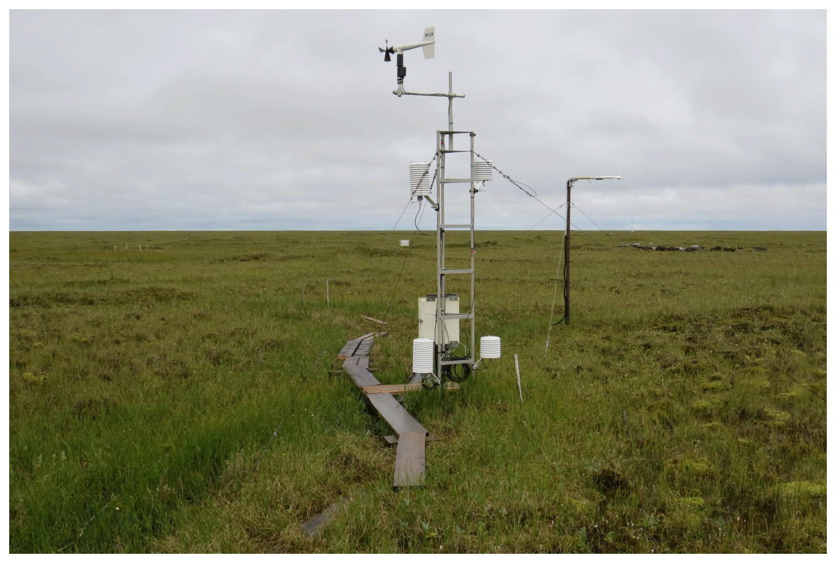
Figure B1Samoylov meteorological station setup, August 2002–present (72.37001∘ N, 126.48106∘ E). Photo taken in August 2015. The two long radiation shields (left side of tower) at heights of 0.5 and 2 m house the combined temperature and relative humidity probes (two Vaisala HMP155A sensors were installed on 17 September 2017) and the two shorter shields (right side of tower) at the same heights contain Campbell Scientific PT100 sensors (installed on 22 August 2013) to measure air temperature only. The data logger (Campbell Scientific CR1000, installed on 30 June 2009), multiplexer (Campbell Scientific AM16/32A, installed on 27 July 2010) and barometric pressure sensor (Vaisala PTP110, installed on 22 August 2014) are located in the white box at the back of the tower. The wind monitor and radiation sensor are shown in the figures below (Figs. B2 and B3).
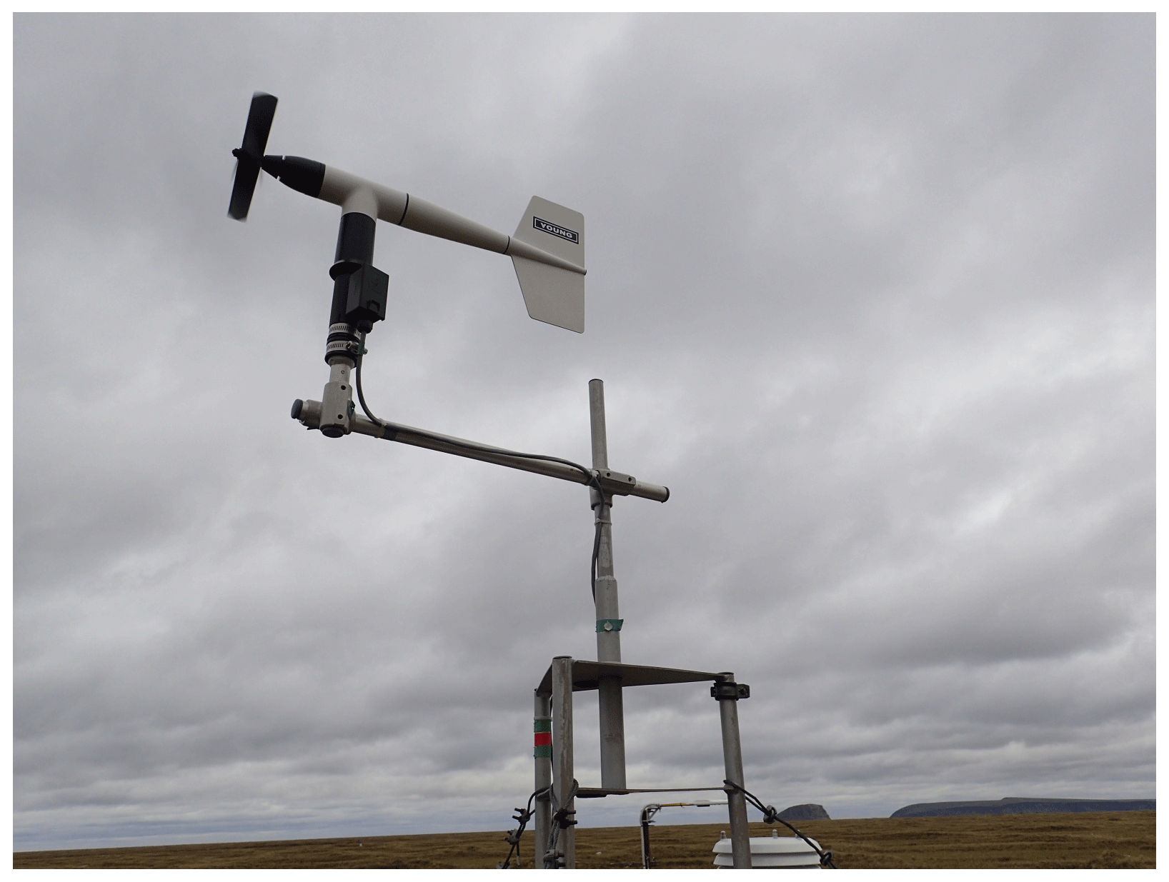
Figure B2Young 05103 wind monitor for measuring wind direction and speed, installed on 31 August 2002.

Figure B3Kipp & Zonen CNR4 radiation sensor (including CNF4 ventilation unit) for measuring incoming and outgoing shortwave and longwave radiation installed on 22 August 2014.
Figure B4Campbell Scientific SR50 snow depth sensor, installed on 24 August 2002. An aluminum plate was installed on the ground surface beneath the sensor beam on 17 July 2015.
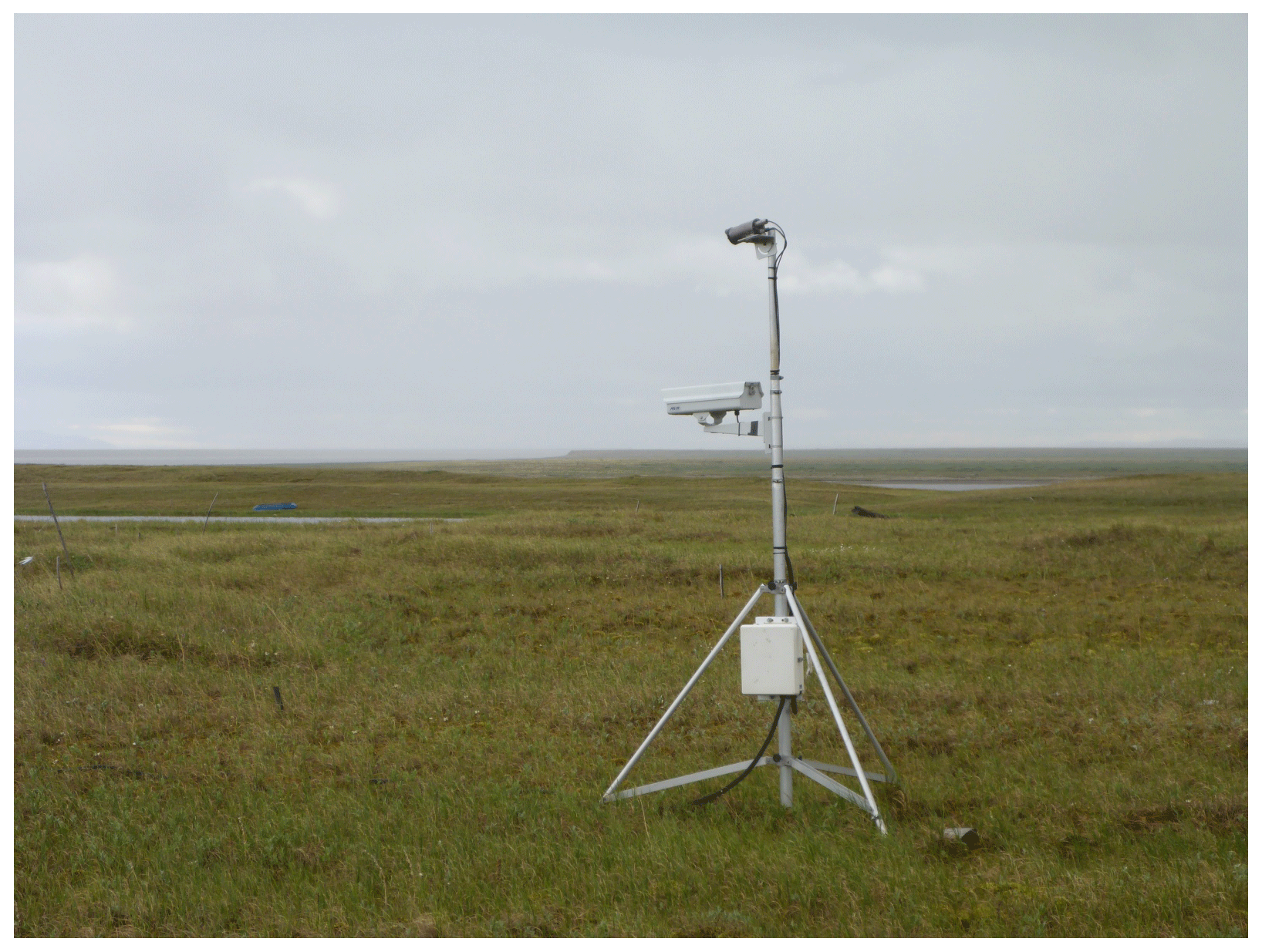
Figure B5Cameras for time-lapse photography of snow cover and land surface pointing towards the polygon field: a Campbell Scientific CC5MPX at the top (since 4 August 2015) and a Campbell Scientific CC640 below (since 1 September 2006). Photo taken in 2016.

Figure B6Examples of photos taken by the cameras used for time-lapse photography (Fig. B5) showing summer field conditions. (a) Left photo taken by the Campbell Scientific CC640 camera (at a height of 2.2 m) and (b) right photo taken by the Campbell Scientific CC5MPX camera (at a height of 3 m) on 7 August 2017.
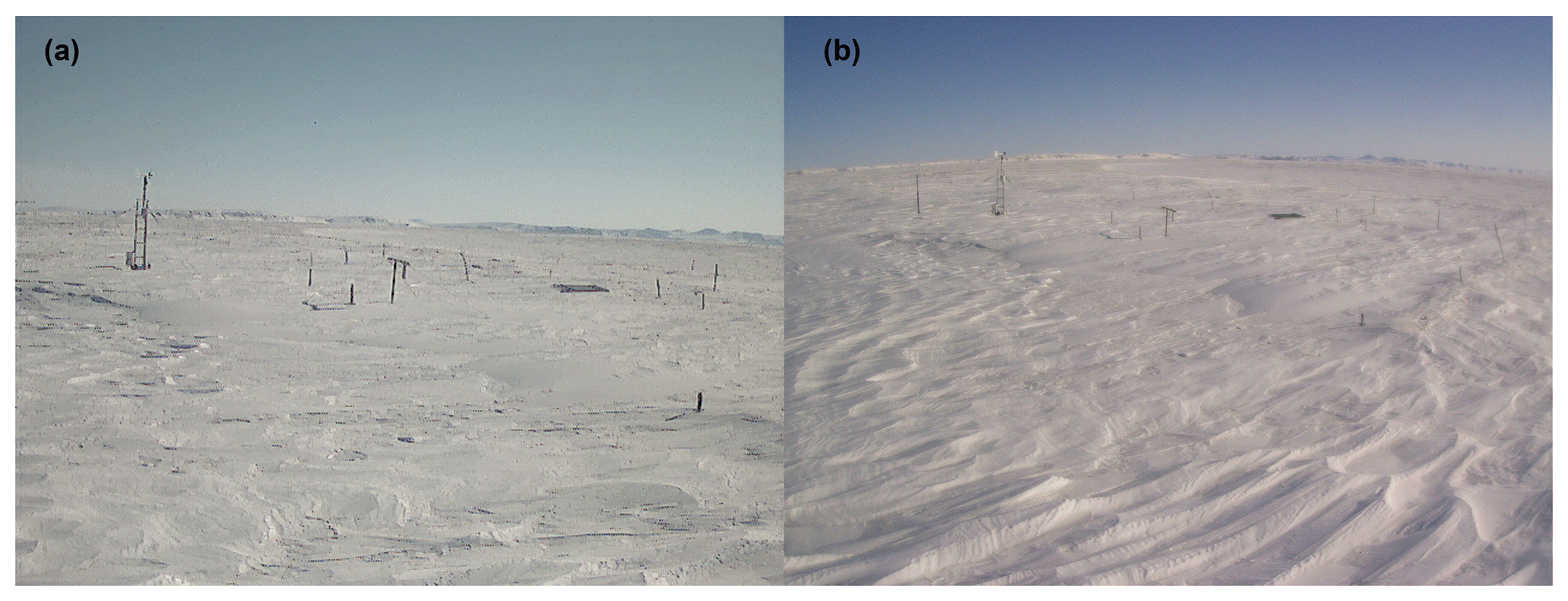
Figure B7Examples of photos taken by cameras used for time-lapse photography (Fig. B5) showing winter field conditions. (a) Left photo taken by the Campbell Scientific CC640 camera (at a height of 2.2 m) and (b) right photo taken by the Campbell Scientific CC5MPX camera (at a height of 3 m) on 4 April 2017.
B2 Soil station
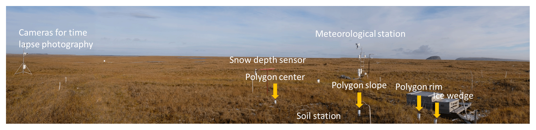
Figure B8Meteorological station and soil station (consisting of sensors installed along 1-D profiles within polygon centre, rim, slope, and ice wedge) with cameras for time-lapse photography pointing towards both stations for snow and surface observations.
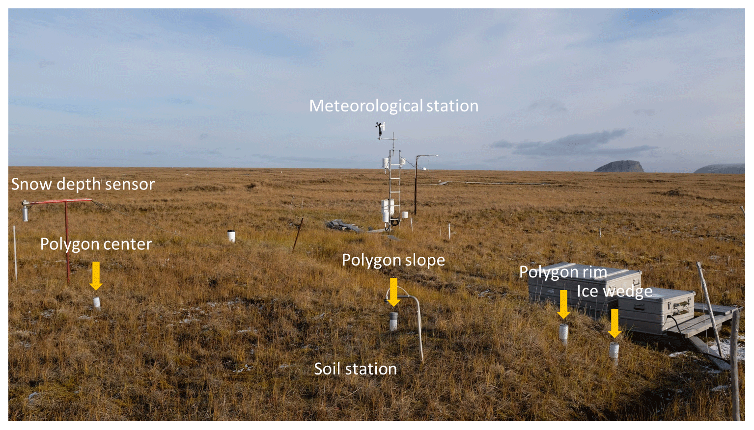
Figure B9Samoylov research site in September 2017, showing locations of meteorological station and soil station (consisting of sensors installed along 1-D profiles within polygon centre, rim, slope, and ice wedge). White/grey tubes have been placed on the surface to indicate the locations of the subsurface sensors and their respective microtopographic locations (polygon centre, rim, slope, and ice wedge).

Figure B10Research site after instrument installation in soil pits and subsequent refilling, August 2002. Cable strings indicate locations of centre, slope, and rim profiles.
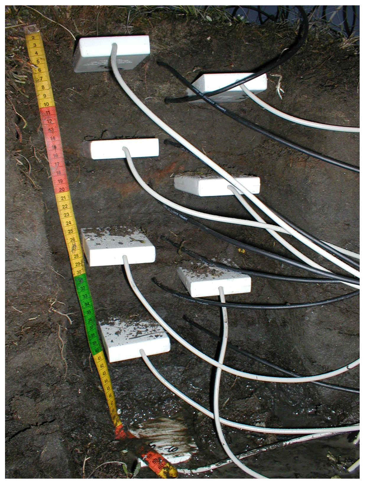
Figure B11Soil volumetric liquid water content sensors (rim): 20 Campbell Scientific CS605 TDR probes, which are connected to a Campbell Scientific TDR100 time-domain reflectometer, installed on 24 August 2002.
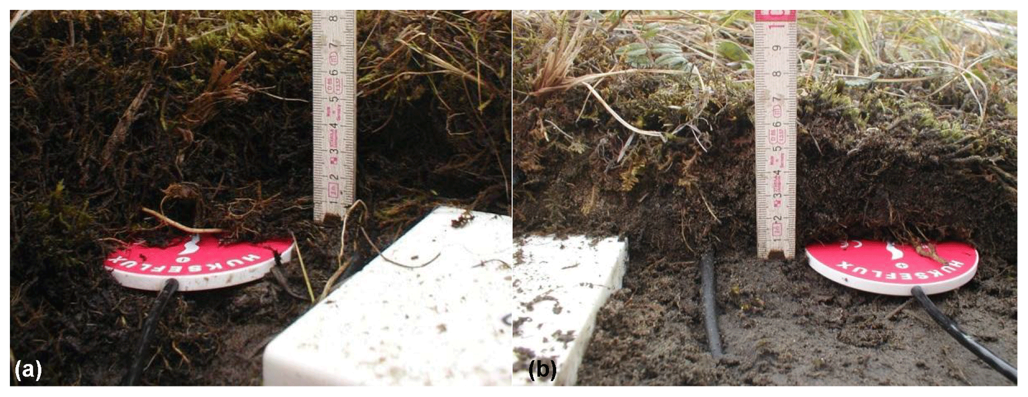
Figure B12Hukseflux HFP01 ground heat-flux sensors (a: centre, b: rim), installed on 24 August 2002.
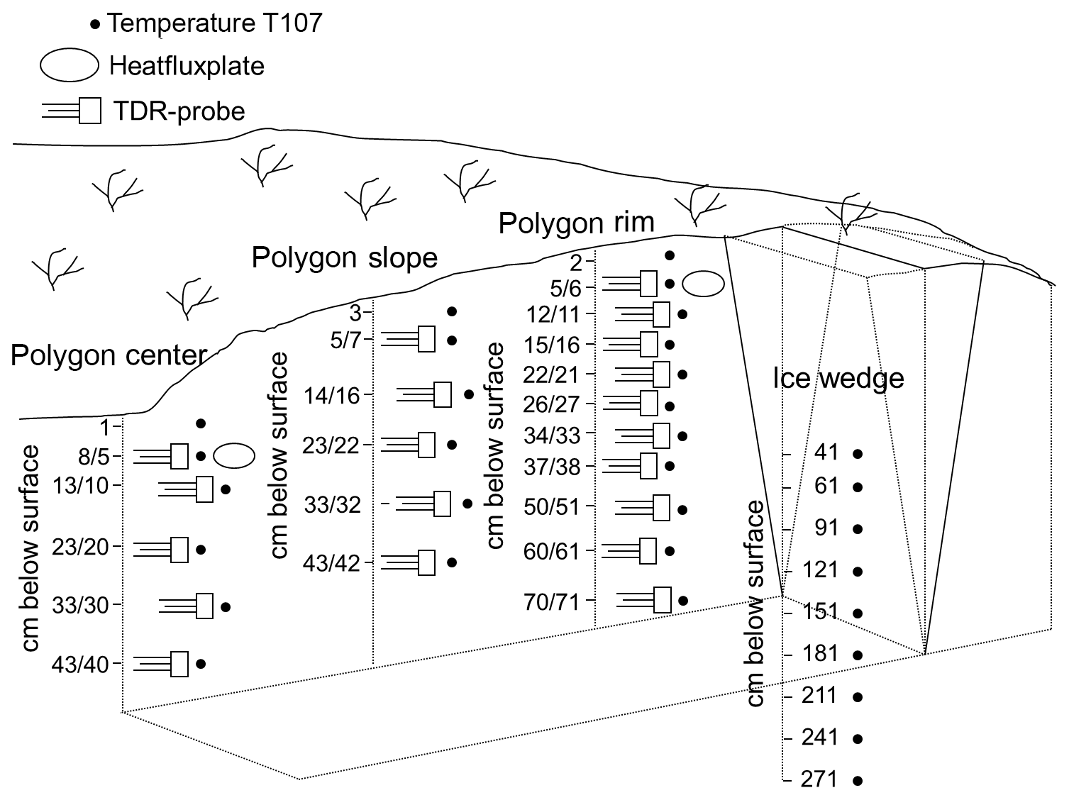
Figure B13Diagram showing the sensor distribution below the polygon's centre, slope, rim and inside the ice wedge, as installed on 24 August 2002. Descriptions of soil profiles and data from these profiles are provided in Appendix F.
C1 Calculation of soil volumetric liquid water content using TDR
The apparent dielectric numbers were converted into liquid water content (θl) using the semi-empirical mixing model in Roth et al. (1990). Frozen soil was treated as a four-phase porous medium composed of a solid (soil) matrix and interconnected pore spaces filled with water, ice, and air.
The TDR method measures the ratio of apparent to physical probe rod length (), which is equal to the square root of the bulk dielectric number (εb).
The bulk dielectric number is then calculated from the volumetric fractions and the dielectric numbers of the four phases using
A value of 0.5 was used for α. It is not possible to distinguish between changes in the liquid water content and changes in the ice content with only one measured parameter (εb). Equation (C1) was therefore rewritten in terms of the total water content (θtot) and the porosity (Φ) as
Note that Equation C2 assumes the densities of liquid and frozen water to be the same, which is clearly incorrect for free phases and probably also in the pore space of soils. However, the density ratio can be absorbed into the dielectric number εi, which we do below. The resulting fluctuation of εi is presumed to be small compared to other uncertainties.
Table C1Porosity values for different depths and locations used for the calculation of volumetric liquid water content. Values were estimated using measured laboratory values, soil texture/horizon characteristics and TDR values at maximum saturation (porosity).
We use
and
to obtain the equation
For temperatures above a threshold freezing temperature (T>Tf), all water is assumed to be unfrozen (θtot=θl). Equation (C5) then reduces to the following:
For temperatures equal to or below the threshold freezing temperature (T≤Tf) it was assumed that the total water content (θtot) remained constant and only the ratio between volumetric liquid water content (θl) and volumetric ice content (θi) changed. This is a rather bold assumption as freezing can lead to high gradients of matric potential, as well as to moisture redistribution. However, since the dielectric number of ice is much smaller than the dielectric number of liquid water, the error in liquid water content measurements is still acceptable (which is not the case for ice content measurements). Under these assumptions we obtained the following equation for calculating the liquid water content of a four-phase mixture:
The error of the volumetric water content measurements using TDR probes was estimated to be between 2 % and 5 %, which is in agreement with Boike and Roth (1997).
The availability of reliable temperature data is crucial in this approach. The liquid water content is first calculated for all times that the soil temperature was above the freezing threshold, using Eq. (C5). When the soil temperature was below the freezing threshold the water content was determined immediately prior to the onset of freezing and used as the total water content (θtot) for calculating the liquid water content during the frozen interval with Eq. (C7).
Since water in a porous medium does not necessarily freeze at 0 ∘C but at a temperature that depends on the soil type and water content, estimating the threshold temperature is a crucial part of this approach. If the freezing characteristic curve is known for the material, then the threshold temperature can be determined from the soil volumetric liquid water content. To avoid interpretations of frequent freezing and thawing due to soil temperature measurement errors, short-term temperature fluctuations were smoothed by calculating the mean of a moving window with an adjustable width. The smoothed temperatures were then used to trigger the switch from one equation to the other, rather than using the original temperature time series.
The porosity values for volumetric liquid water content calculations were obtained from laboratory measurements (Appendix F) and adjusted for probe location if necessary.
C2 Snow depth correction for air temperature
The acoustic distance sensor (Campbell Scientific SR50) measures the elapsed time between emission and return of the ultrasonic pulse. The raw distance Dsnraw obtained from the sensor was temperature corrected using the speed of sound at 0 ∘C and the air temperature at 2 m height (Tair_200) in Kelvin (K), using the formula provided by the manufacturer (Campbell Scientific, 2007):
A measurement system was installed in a polygon centre 3 m southeast of the meteorological station tower at 72.37001∘ N, 126.48106∘ E to allow changes in the water level to be recorded without requiring the presence of any personnel. A major disadvantage of using a common pressure transducer sensor to measure the water level is that such a device cannot withstand the long frozen Arctic winter and is therefore not suitable for use when the presence of personnel is limited due to expedition schedules being restricted to the summer period. A setup that can remain installed and withstand the cold winter temperatures therefore has a great advantage.

Figure D1Scheme of setup of water-level measurement in the polygon centre: (a) length of the parallel measurement rods (30 cm) of the Campbell Scientific CS616–CS625 sensors, (b) distance from the sensor base to the ground surface (CS625 is −15 cm; CS616 is −11.5 cm), (c) Campbell Scientific T109 probes at depths of −1, −3, and −6 cm below the surface, (d) height of the well above the ground surface (45.5 cm), (e) length of the well (70 cm), (f) distance from the top of the well to the water pressure measurement level of the Schlumberger Mini-Diver. The difference between the ground level at CS616 and Mini-Diver locations is 3 cm. Blue line illustrates water level, grey line the ground surface.
We apply vertically installed soil moisture probes to estimate water level, as described in Thomsen et al. (2000). Our sensors remained permanently in the soil with the circuit board at the base of the sensor and the parallel-connected rods pointing upwards. The base of the sensor marks the lowest measurable water level. For the water content reflectometer we measured the distance from the ground surface to the base of the sensor, where the measurement rods are connected (Fig. D1), to compute water level below the ground surface. From 2007 to 2010 a Campbell Scientific CR200 data logger was connected to a Campbell Scientific CS625 probe (15 cm below the ground surface) to record the water level and two Campbell Scientific T109 sensors (1 and 6 cm below the surface) for temperature measurements. Since 2010 the setup has been connected to the main Campbell Scientific CR1000 logger of the meteorological station and the CS625 probe was therefore exchanged for a Campbell Scientific CS616 probe, installed 11.5 cm below the ground surface. Due to a change in data loggers in the summer of 2010, we have two setups with minor differences in the measurement probes and their installation depths, which is detailed below and visualized in Fig. D1. The difference between the two water content reflectometers is the electrical output voltage, which had to be changed in order to meet the requirements of the logger. A third T109 probe was also installed 3 cm below ground surface in 2010. This setup is still in operation. These temperature data are only used to distinguish between periods of frozen and unfrozen surface conditions. The unfrozen period, for which water levels were computed, was defined as the period for which soil temperatures at 6 cm below the surface are >0.4 ∘C during spring, and >0.1 ∘C during fall. Below these temperatures, no water-level data are provided.
To obtain a better field calibration of the water content reflectometer a Schlumberger Mini-Diver pressure water-level sensor was installed in a well in the same polygon for 68 days of the non-frozen vegetation period in 2016. Measurements obtained from the Mini-Diver were compensated for changes in air pressure using data from the meteorological station's barometric pressure sensor (Vaisala PTB110).
Calculation and correction of water-level measurements
The measured output, signal period (SP) from the Campbell Scientific CS616 or CS625 probes were converted into the height of the water level above the sensor base (WL) using two polynomial functions derived from an empirical field experiment to determine the correlation between the results from the CS616–CS625 probes and those from a Mini-Diver.
The two regressions represent different water-level regimes (low and higher water levels) recorded by the CS616–CS625 sensor. The results of this experiment showed a low accuracy for very low water levels (1.5 cm or less above the sensor base) resulting in output periods of SP <19 µs, which were excluded from the data series. For values >19 µs, the following formulas are applied to obtain WL data from the CS616 and CS625 probe output:
for SP <27 µs and
for SP >27 µs. Note that WL for the equations above is given in centimetres.
The mean deviation of the calculated WL values from the values measured with the Mini-Diver was (0.034 cm) with a standard deviation of 0.29 cm (number of values: 2679).
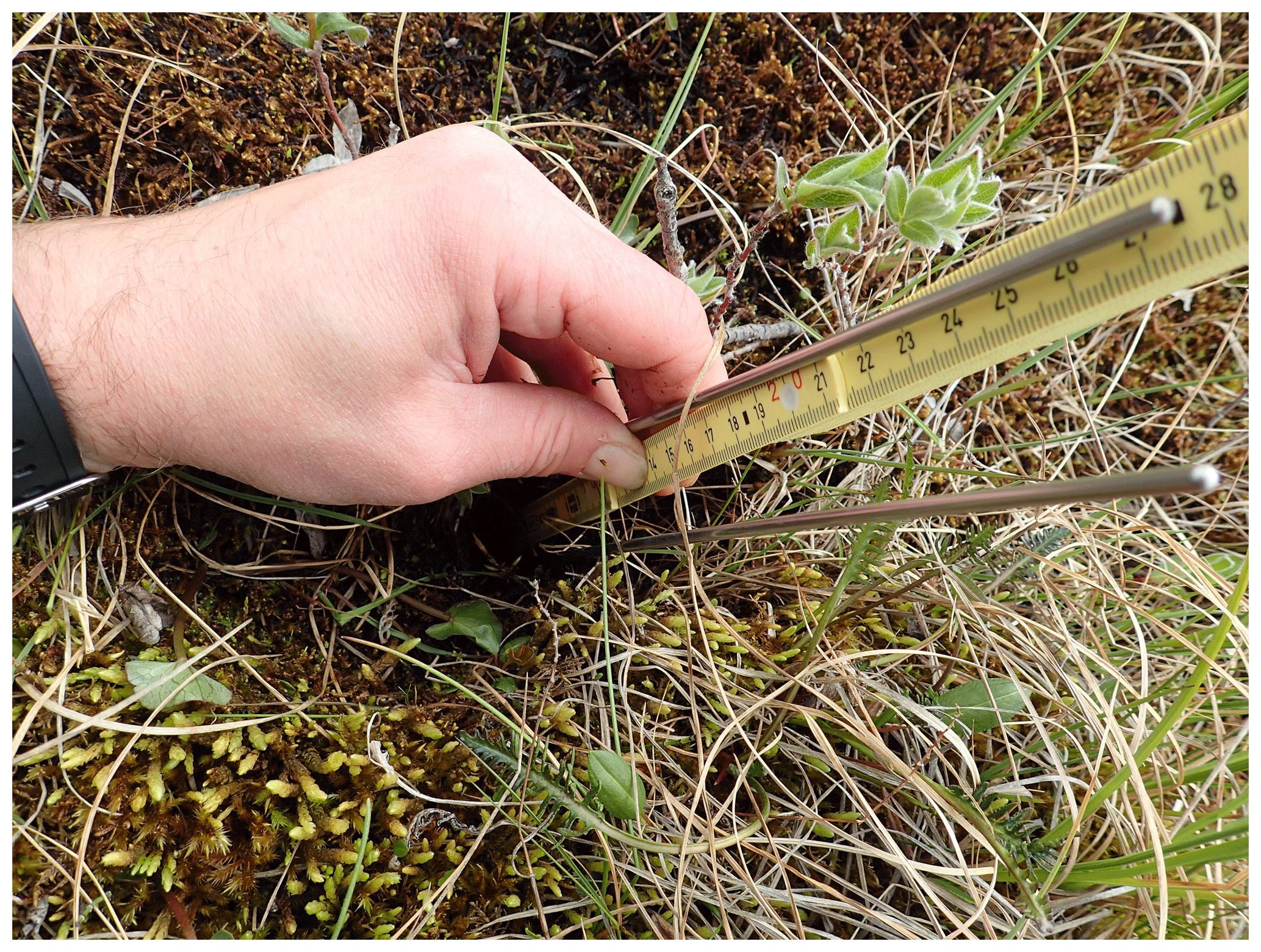
Figure D2Campbell Scientific CS616 vertical probe installation. Water-level measurement is done manually with a ruler.
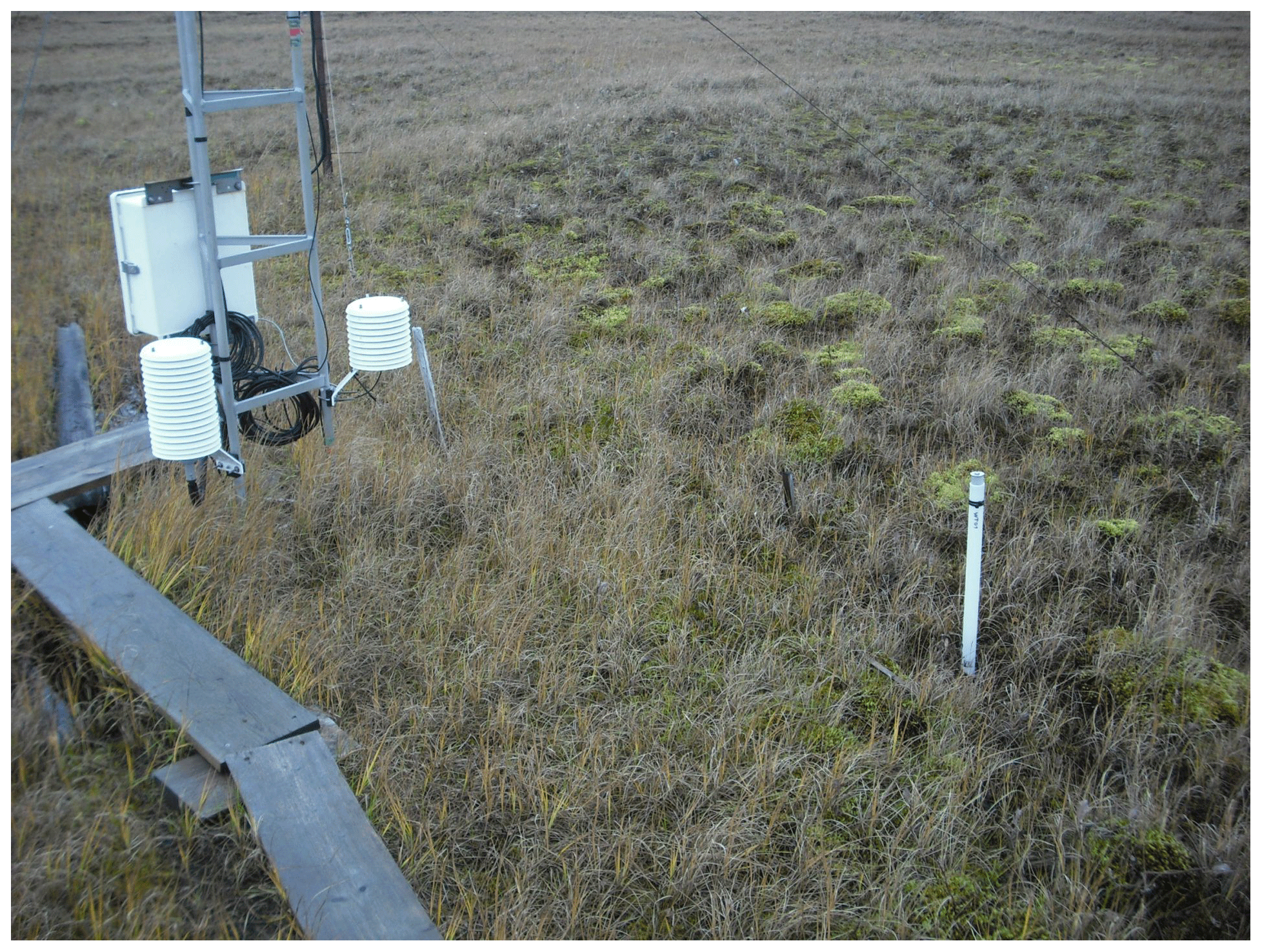
Figure D3Installation for water-level measurements using a permeable ground water measurement tube with a Schlumberger Mini-Diver.
Note that WL is given relative to the sensor base in the time series data and
reported in metres. To obtain water level relative to the ground surface
(WLgs) from level 1 data, the following calculation is suggested for CS616:
For CS625,
Special post-processing of the CS625 sensor readings was carried out from 6 July 2009 to 26 July 2010, as no probe output periods were logged over this period. Instead, volumetric liquid water content (θl) was stored on the CR200 logger and calculated from the CS625 probe output using a formula from the sensor's manual (Campbell Scientific, 2016). The θl, values were converted to SP values using formula (D5):
We compared the calculated WL with manual distance measurements taken in the field over the years (n=12). The largest differences between TDR-derived and manual measurements was 2 cm. This includes all measurement errors, such as sensor movement (probes are not anchored into the permafrost, they can potentially move with the seasonal heaving, subsiding of the active layer), and difficulties in defining the ground surface (which is covered by mosses and grasses).
A borehole was drilled at 72.36941∘ N, 126.47612∘ E into the permafrost during the spring of 2006. Drilling started with 146 mm diameter to 4 m depth and continued with 132 mm diameter to 26.75 m depth. A 4 m long metal stand pipe (diameter 13 cm) was used for stability and to prevent the inflow of water during the summer season into the borehole. The metal pipe extends 0.5 m above and 3.5 m below the ground surface (Figs. E1 and E2).
A thermistor chain with 24 temperature sensors (RBR thermistor chain with an XR-420 logger) was inserted into a close-fitting PVC tube (4 cm inside, 5 cm outside diameter) and installed in the borehole on 21 August 2006, down to a depth of 26.75 m (Fig. E2).
A second PVC tube with the same dimensions as the first tube was also inserted into the borehole to permit additional (geophysical and calibration) measurements to be made in the future. The remaining air space in the borehole was backfilled with dry sand. The outside metal pipe (used for drilling and to prevent inflow of water), which stands 0.5 m above the ground surface, was closed at the top, and was covered with a wooden shield which was renewed in 2015.
The accuracy of the temperature sensors of the thermistor chain is reported by RBR to be ±0.005 ∘C between −5 and 35 ∘C. However, direct comparison with a high-precision reference PT100 temperature sensor (certified to be accurate to ±0.01 ∘C between −20 and 30 ∘C) at six different depths in the borehole between 9 and 17 August 2014 showed the accuracy of the RBR XR-40 temperature sensors to be approximately ±0.03 ∘C at depths ≥8.75 m (Table E1). The deviation increased with decreasing depth; e.g. between −7.75 and -1.75 m the deviation was ±0.33 ∘C and at −0.75 m it was ±0.65 ∘C. This increase in deviation towards the surface may be because (a) the chain was installed in sand, whereas the calibration thermometer was in air and could therefore possibly have been affected by air circulation, or (b) the temperature gradient becomes steeper with decreasing depth below the surface and thus small differences between the measuring heights of the two sensors will have a larger impact on temperatures as the surface is approached. The offset of the reference thermometer at exactly 0 ∘C was 0.01 ∘C, and the average statistical accuracy (Uk=2) is given by the manufacturer as 0.1083 ∘C. During calibration in the borehole the temperature was given time to stabilize (i.e. until the recorded temperature change was less than ±0.03 ∘C) before being recorded (Table E1).
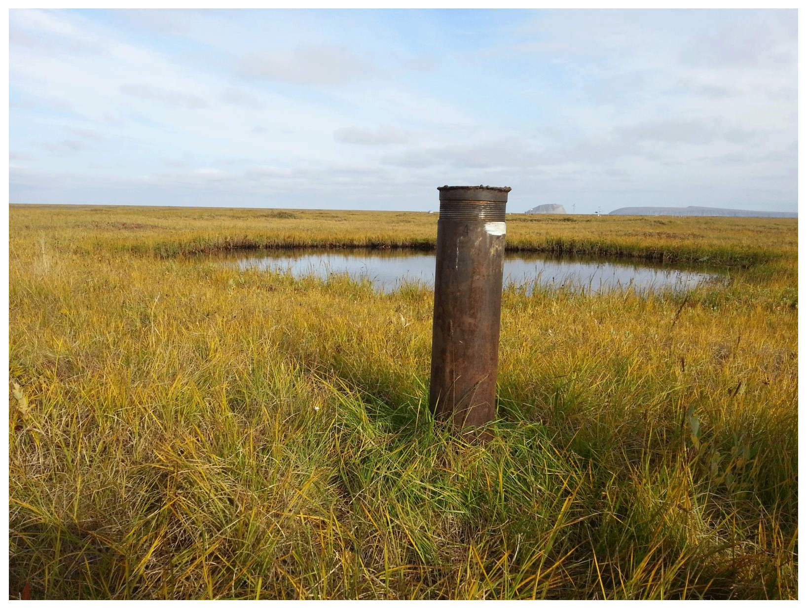
Figure E1Location of the 2006 borehole showing the proximity of the borehole to a small lake. The metal pipe extends 0.5 m above the ground surface.
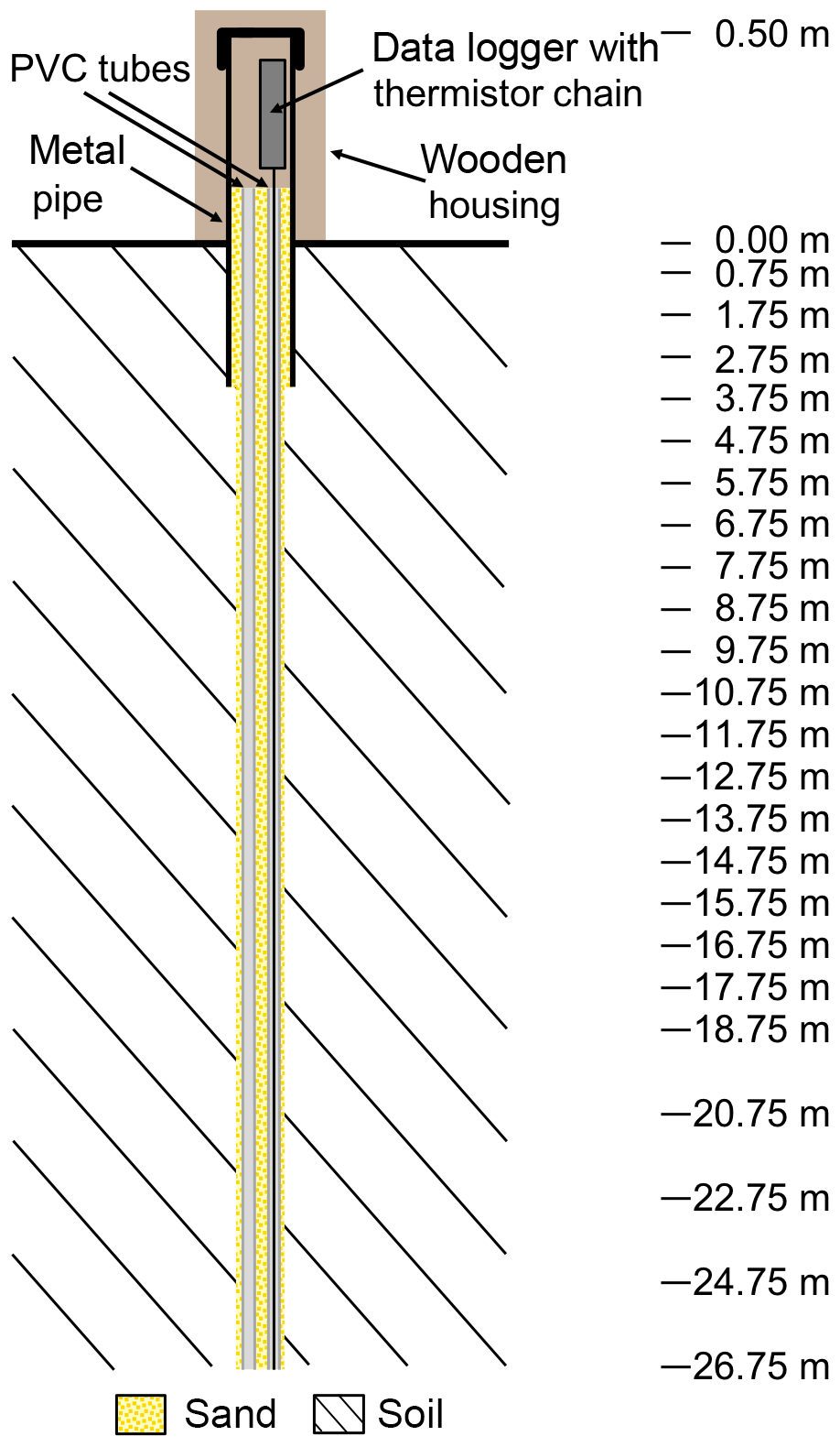
Figure E2Thermistor setup showing their depths within the borehole, as installed in 2006. The metal pipe extends 0.5 m above ground surface. Note the differences in scale above and below the ground surface.
Continuous measurements have been obtained since mid-August 2006 from sensor depths of 0.00, 0.75, 1.75, 2.75, 3.75, 4.75, 5.75, 6.75, 7.75, 8.75, 9.75, 10.75, 11.75, 12.75, 13.75, 14.75, 15.75, 16.75, 17.75, 18.75, 20.75, 22.75, 24.75, and 26.75 m below the ground surface. We recommend that the temperature data from the three sensors at 0, 0.75, 1.75 and 2.75 m depths should not be used due to the possibility of them having been affected by the metal access pipe. The data from these sensors have not been flagged as they are of high quality, but they may not provide an accurate reflection of the actual soil temperatures.
Table E1In situ calibration of thermometers in the borehole between 9 and 17 August 2014. Comparison measurements were made in the 27 m borehole using a certified PT100 thermometer (Service für Messtechnik Geraberg DTM 3000).
Construction of the new Russian Samoylov Island Research Station started in September 2011 and was completed in summer 2012. The new research station included a water supply from a nearby lake. The water supply system (Figs. E3 and E4) is an aboveground structure that is likely to affect the wind and hence the accumulation of snow on the tundra surface. Visual inspection in the vicinity of the borehole in April 2016 suggested an increased snow accumulation around this location since construction of the water supply system. A new borehole was drilled in April 2018 down to 61 m, far away from the research station and associated structures. A new temperature chain was installed in the early summer of 2018 to provide deeper permafrost data, as well as observations from a second borehole.
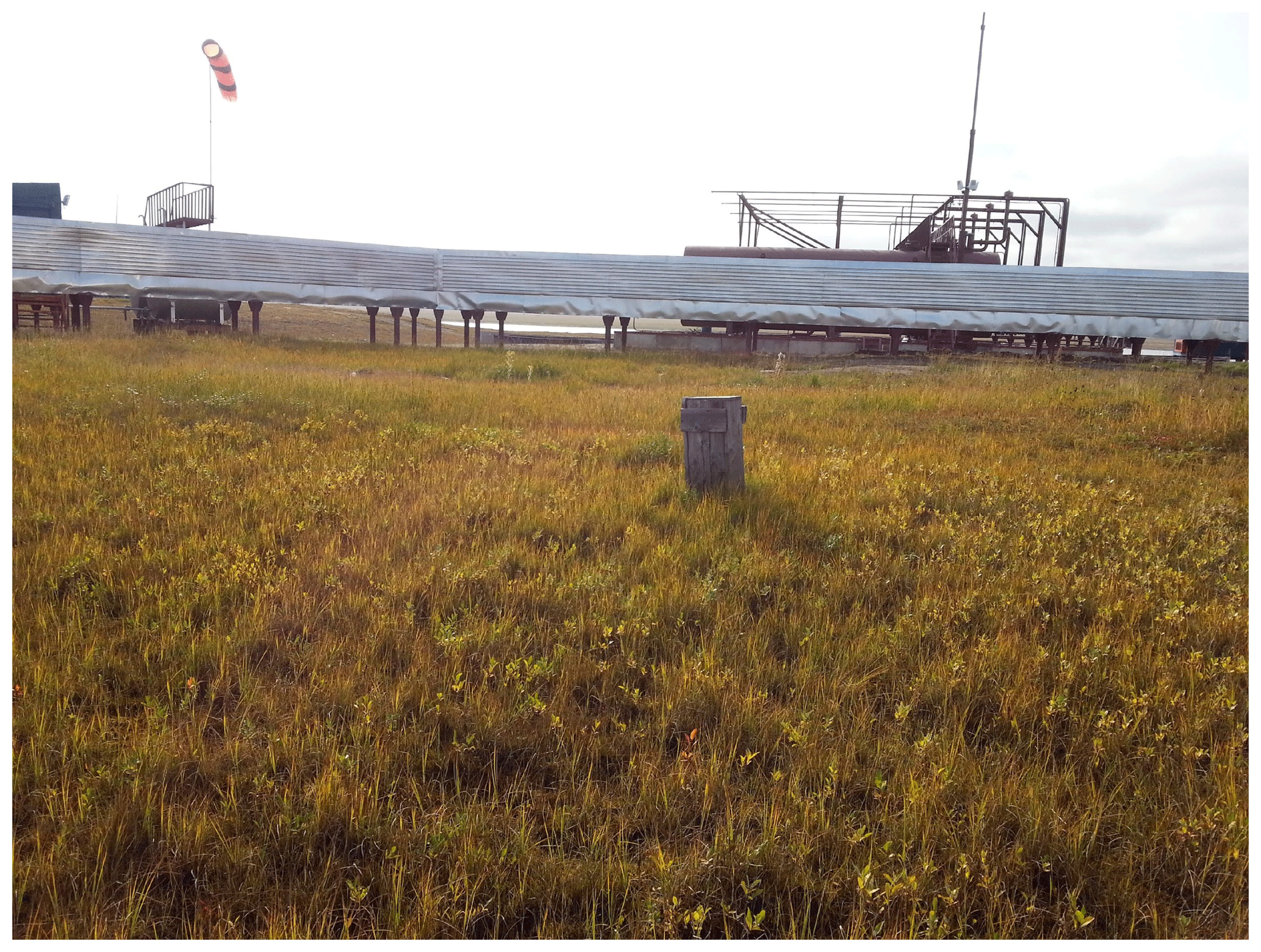
Figure E3Location of the 2006 borehole (wooden box) showing the proximity of the new water supply system (a silver metal structure extending above the tundra surface since 2013).
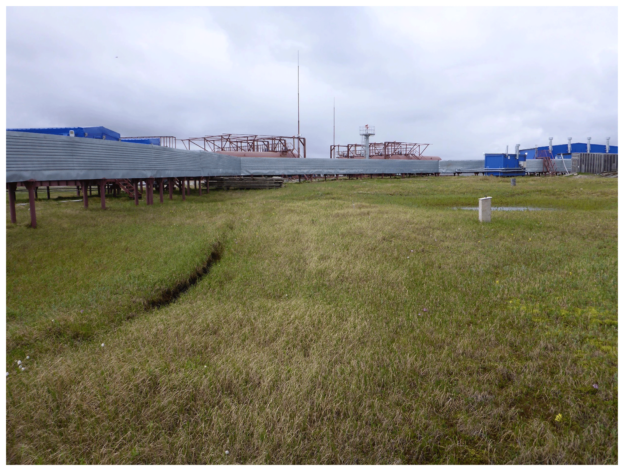
Figure E4Borehole location (wooden box on right side) with the new Samoylov research station and water supply system (silver metal structure extending above the tundra surface).
The organic carbon density in bulk soil CDbulk (kg m−3) was calculated using the mass fraction of organic carbon in soil OC, the average dry bulk density , and the following formula:
Table F1Soil data from the BS-1 (polygon rim) and BS-3 (polygon centre) soil pits, which were sampled and had instruments installed in 2002. The location of the soil profiles is described in Wille et al. (2003) and shown in Figs. B8 and B9. Photos of the soil profiles can be seen in Fig. F1 below. Grain size classification is according to Folk (1954), where S is sand, s is sandy, Z is silt, z is silty, M is mud, m is muddy, C is clay, and c is clayey. Other abbreviations used are OC for the mass fraction of organic carbon in soil, N for the mass fraction of nitrogen in soil, CDbulk for the organic carbon density in bulk soil, and SOCC for the soil organic carbon content for each soil horizon. The soil horizon designations are according to the USDA Soil Survey Staff (2010). The BS-1 and BS-2 (polygon slope) soil profiles are classified as Typic Aquiturbels and the BS-3 soil profile is classified as Typic Historthel according to the US Soil Taxonomy (Soil Survey Staff, 2010). Analysis of the physical properties of soil was done according to DIN 19683 (1973). OC and N were determined following the removal of inorganic carbon and dry combustion at 900 ∘C (DIN ISO 10694).

The organic carbon content for each soil horizon SOCC (kg m−2) was calculated using the mass fraction of organic carbon in soil OC, the average dry bulk density , the horizon thickness, and the following formula:
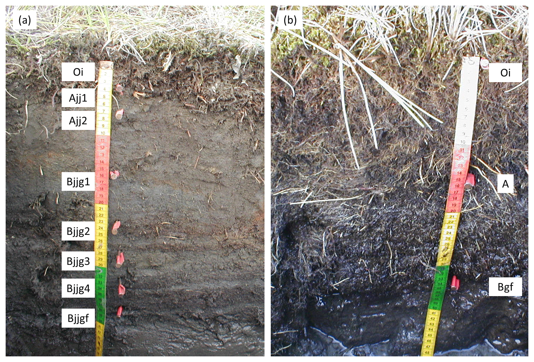
Figure F1Photographs of soil profiles (a) BS-1 (Typic Aquiturbel) at the peak of a polygon rim and (b) BS-3 (Typic Historthel) at a polygon centre. Designations of soil horizons according to US Soil Taxonomy (Soil Survey Staff, 2010). Horizon labels are positioned at the upper boundary of the respective horizon.
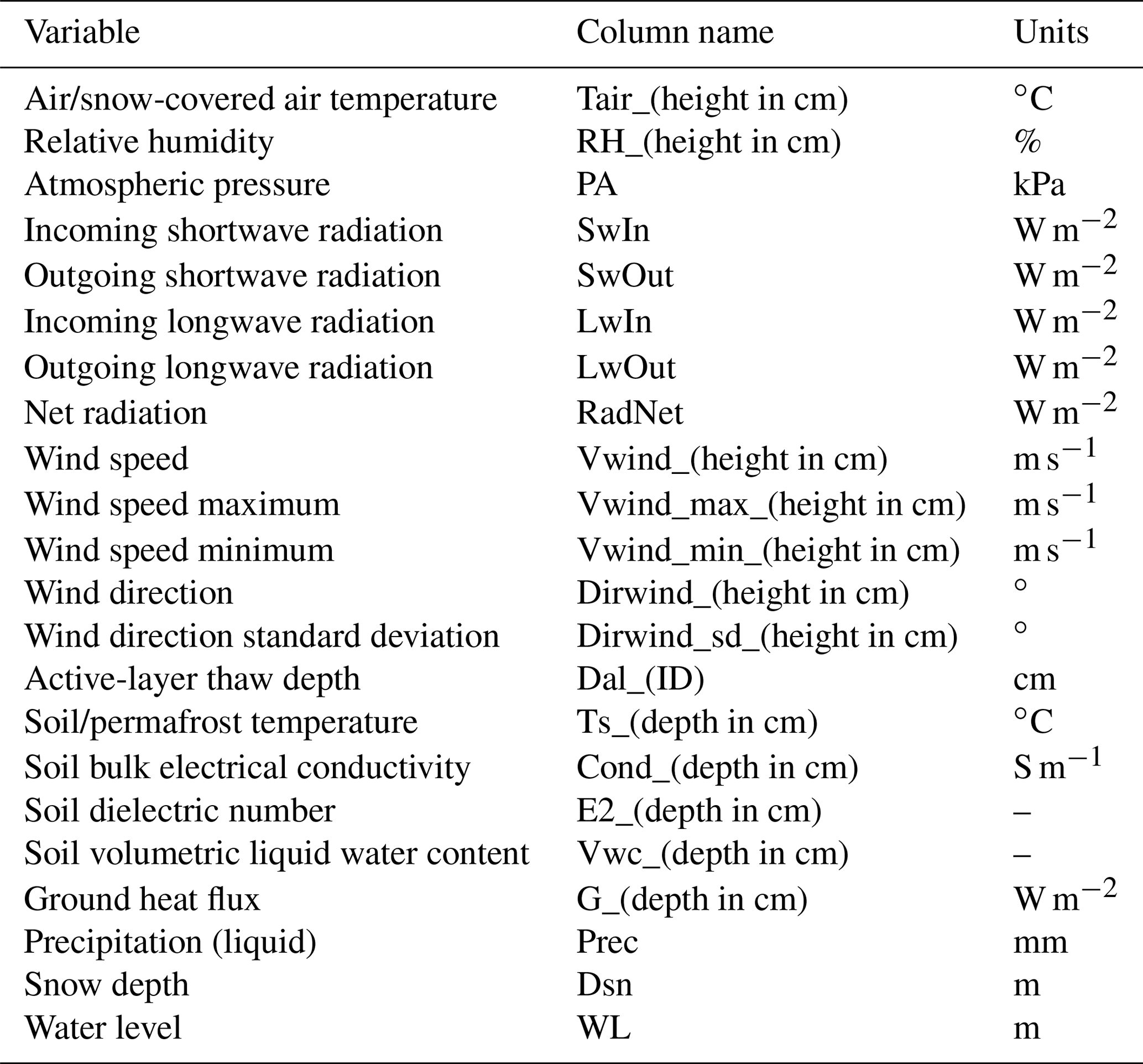
Table G1Overview of all variables published as a time series. Some variables have _center, _rim and _slope as their location index (Sect. 3.2). Additional level 2 data are published for the variables air temperature, relative humidity, precipitation, wind speed and direction, net radiation, soil temperatures, and soil volumetric liquid water content, which is indicated by _lv2 in the column name. If an air temperature sensor is covered by snow and thus measures snow temperature, this is indicated by a Flag 8 in the data.
3-D point cloud data were acquired for several polygons around the meteorological, soil and CALM sites by terrestrial laser scanning (TLS) on 12 September 2017, using a RIEGL VZ-400 3-D TLS instrument. According to the manufacturer's specifications, the TLS instrument measures 3-D coordinates with an accuracy of 5 mm and a precision of 3 mm (RIEGL LMS, 2017). We captured the full extent of the research site, which has dimensions of approximately 70×70 m, from 10 scan positions with a horizontal and vertical point spacing of 3 mm at 10 m measurement range. The single-point clouds were registered into a common coordinate system using five cylindrical reflectors placed around the research site during the TLS data acquisition so that they were visible from all scan positions. Mean residual distances per scan position between the cylindrical reflectors amounted to 1.6 cm, with a standard deviation of 0.8 cm.
The registered 3-D point cloud data set was georeferenced using high-accuracy global positioning measurements recorded with a global navigation satellite system (GNSS). We obtained GNSS measurements in static-phase observation mode with a Leica Viva GS10 as the base station receiver and a GS15 mobile rover unit (Leica Geosystems, 2012a, b). According to the manufacturer's specifications (Leica Geosystems, 2012a), this mode achieves a measurement accuracy of 3 mm horizontally and 3.5 mm vertically with respect to the local reference frame established by the base station. The scan positions were georeferenced and registered using the RiSCAN PRO software (version 2.1.1; RIEGL LMS, 2016).
The raw data set was filtered using a statistical outlier removal (SOR; Rusu and Cousins, 2011) to remove spatially isolated points as outliers from the point cloud, with the number of neighbours set to 10 and the standard deviation multiplier threshold to 1.0.
A digital terrain model (DTM) representing the ground-surface elevation was derived from this preprocessed data set. To determine the ground-surface elevation the 3-D TLS points were first classified into ground and non-ground points. For this we used a minimum approach, classifying all points within a search radius of 2.5 cm that were at less than 1.0 cm vertical distance from the minimum point elevation as ground points. This vertical distance threshold is included to take into account position uncertainties of the TLS acquisition. The ground points in the 3-D TLS data set are subsequently rasterized into the final DTM (with a cell size of 5.0 cm) using a robust moving-plane interpolation strategy (TU Wien, 2016).
For evaluation purposes the DTM was compared to 27 GNSS measurements of the ground surface that were obtained during the TLS data acquisition. The data sets were compared by taking the difference between GNSS-based elevation measurements and the corresponding DTM pixel values. Statistical analysis of these differences in ground-surface elevation yielded a mean difference of 3.7 cm, a median difference of 1.7 cm, and a standard deviation of 5.1 cm. Differences were mainly within the accuracy ranges of TLS point cloud registration and GNSS positioning. Larger positive differences (>2.0 cm) indicated an overestimation of ground-surface elevation in the TLS point cloud. Where dense, short vegetation is present, an error is introduced to the estimated ground-surface elevation as the laser beam does not hit the ground surface at every local area in the site. This is to be expected, particularly for larger distances from the scan positions, as the incidence angle from the TLS instrument has a direct effect on the penetration depth of the laser beam (Marx et al., 2017).
Relative height above the ground surface was derived as vertical distance of TLS points to the ground surface. The DTM was used to calculate the vertical distance to the ground surface for every 3-D point in the TLS point cloud. A raster of relative height values was generated using the 99th percentile of the relative height attribute per raster cell, with a cell size of 5.0 cm. Furthermore, a raster of mean relative heights above the ground surface was generated that could provide an estimate of the vegetation height and volume within each 5 cm raster cell. With regard to the vegetation height values derived from the TLS data, it should be noted that the heights could be underestimated when compared to actual field measurements, for which there are two possible explanations. Firstly, overestimation of the ground-surface elevation (where the laser beam does not fully penetrate the vegetation) reduces the calculated relative (vegetation) height. Secondly, the sampling of the laser-scanning process with the given 3-D point spacing implies an uncertainty in the maximum height being recorded at every local position. This applies in particular to grass-covered surfaces, where individual blades are not necessarily hit by the laser beam at their highest point. Both of these effects can result in reduced vegetation heights in a TLS-based approach, e.g. compared to length measurements of individual sedges in the field.
The modular programme system OPALS (version 2.3.0; Pfeifer et al., 2014) was used for the point cloud analyses of ground-surface elevation and relative height above the ground surface.
JB initiated and set up the long term observational site on Samoylov together with LK and CW. Data collection was done by JB, CW, NB, and PS, with the support of MG, DB, and AM. KA collected the terrestrial lidar scanning data and analysed the data. IG, SC, and ML contributed to the modelling sections, EB and SC provided the Samoylov driving data. JB wrote the paper with inputs from the co-authors and coordinated the analysis and contributions from all co-authors.
The authors declare that they have no conflict of interest.
Logistical support was provided by the Russian–German
Samoylov Research Base (1998–2012) and the Russian Samoylov Island Research
Station (2013–2017). Field support, including data collection, was provided
by Konstanze Piel, Steffen Frey, Günter Stoof, and Waldemar Schneider.
We gratefully acknowledge the funding received from the Helmholtz
Association's ACROSS (Advanced Remote Sensing – Ground Truth Demo and Test
Facilities) project.
Edited by: Kirsten Elger
Reviewed by: Richard L. H. Essery and Nick Brown
Aalto, J., Karjalainen, O., Hjort, J., and Luoto, M.: Statistical Forecasting of Current and Future Circum-Arctic Ground Temperatures and Active Layer Thickness, Geophys. Res. Lett., 45, 4889–4898, https://doi.org/10.1029/2018GL078007, 2018.
Aas, K. S., Martin, L., Nitzbon, J., Langer, M., Boike, J., Lee, H., Berntsen, T. K., and Westermann, S.: Thaw processes in ice-rich permafrost landscapes represented with laterally coupled tiles in a land surface model, The Cryosphere, 13, 591–609, https://doi.org/10.5194/tc-13-591-2019, 2019.
Abnizova, A., Siemens, J., Langer, M., and Boike, J.: Small ponds with major impact: The relevance of ponds and lakes in permafrost landscapes to carbon dioxide emissions, Global Biogeochem. Cy., 26, GB2041, https://doi.org/10.1029/2011gb004237, 2012.
Abramova, E., Vishnyakova, I., Boike, J., Abramova, A., Solovyev, G., and Martynov, F.: Structure of freshwater zooplankton communities from tundra waterbodies in the Lena River Delta, Russian Arctic, with a discussion on new records of glacial relict copepods, Polar Biol., 40, 1629–1643, https://doi.org/10.1007/s00300-017-2087-2, 2017.
Antonova, S., Sudhaus, H., Strozzi, T., Zwieback, S., Kääb, A., Heim, B., Langer, M., Bornemann, N., and Boike, J.: Thaw Subsidence of a Yedoma Landscape in Northern Siberia, Measured In Situ and Estimated from TerraSAR-X Interferometry, Remote Sensing, 10, 494, https://doi.org/10.3390/rs10040494, 2018.
Beringer, J., Lynch, A. H., Chapin, F. S., Mack, M., and Bonan, G.: The Representation of Arctic Soils in the Land Surface Model: The Importance of Mosses, J. Climate, 14, 3324–3335, https://doi.org/10.1175/1520-0442(2001)014<3324:TROASI>2.0.CO;2, 2001.
Biskaborn, B. K., Smith, S. L., Noetzli, J., Matthes, H., Vieira, G., Streletskiy, D. A., Schoeneich, P., Romanovsky, V. E., Lewkowicz, A. G., Abramov, A., Allard, M., Boike, J., Cable, W. L., Christiansen, H. H., Delaloye, R., Diekmann, B., Drozdov, D., Etzelmüller, B., Grosse, G., Guglielmin, M., Ingeman-Nielsen, T., Isaksen, K., Ishikawa, M., Johansson, M., Johannsson, H., Joo, A., Kaverin, D., Kholodov, A., Konstantinov, P., Kröger, T., Lambiel, C., Lanckman, J.-P., Luo, D., Malkova, G., Meiklejohn, I., Moskalenko, N., Oliva, M., Phillips, M., Ramos, M., Britta, A., Sannel, K., Sergeev, D., Seybold, C., Skryabin, P., Vasiliev, A., Wu, Q., Yoshikawa, K., Zheleznyak, M., and Lantuit, H.: Permafrost is warming at a global scale, Nat. Commun., 10, 264, https://doi.org/10.1038/s41467-018-08240-4, 2019.
Boike, J. and Roth, K.: Time Domain Reflectometry as a Field Method for Measuring Water Content and Soil Water Electrical Conductivity at a Continuous Permafrost Site, Permafrost Periglac., 8, 359–370, https://doi.org/10.1002/(SICI)1099-1530(199710/12)8:4<359::AID-PPP261>3.0.CO;2-S, 1997.
Boike, J., Ippisch, O., Overduin, P. P., Hagedorn, B., and Roth, K.: Water, heat and solute dynamics of a mud boil, Spitsbergen, Geomorphology, 95, 61–73, https://doi.org/10.1016/j.geomorph.2006.07.033, 2008a.
Boike, J., Wille, C., and Abnizova, A.: Climatology and summer energy and water balance of polygonal tundra in the Lena River Delta, Siberia, J. Geophys. Res., 113, G03025, https://doi.org/10.1029/2007JG000540, 2008b.
Boike, J., Kattenstroth, B., Abramova, K., Bornemann, N., Chetverova, A., Fedorova, I., Fröb, K., Grigoriev, M., Grüber, M., Kutzbach, L., Langer, M., Minke, M., Muster, S., Piel, K., Pfeiffer, E.-M., Stoof, G., Westermann, S., Wischnewski, K., Wille, C., and Hubberten, H.-W.: Baseline characteristics of climate, permafrost and land cover from a new permafrost observatory in the Lena River Delta, Siberia (1998–2011), Biogeosciences, 10, 2105–2128, https://doi.org/10.5194/bg-10-2105-2013, 2013.
Boike, J., Juszak, I., Lange, S., Chadburn, S., Burke, E., Overduin, P. P., Roth, K., Ippisch, O., Bornemann, N., Stern, L., Gouttevin, I., Hauber, E., and Westermann, S.: A 20-year record (1998–2017) of permafrost, active layer and meteorological conditions at a high Arctic permafrost research site (Bayelva, Spitsbergen), Earth Syst. Sci. Data, 10, 355–390, https://doi.org/10.5194/essd-10-355-2018, 2018a.
Boike, J., Nitzbon, J., Anders, K., Grigoriev, M. N., Bolshiyanov, D. Y., Langer, M., Lange, S., Bornemann, N., Morgenstern, A., Schreiber, P., Wille, C., Chadburn, S., Gouttevin, I., and Kutzbach, L.: Measurements in soil and air at Samoylov Station (2002–2017), PANGAEA, https://doi.org/10.1594/PANGAEA.891142, 2018b.
Boike, J., Nitzbon, J., Anders, K., Grigoriev, M. N., Bolshiyanov, D. Y., Langer, M., Lange, S., Bornemann, N., Morgenstern, A., Schreiber, P., Wille, C., Chadburn, S., Gouttevin, I., and Kutzbach, L.: TLS measurements at Samoylov in 2017, link to pointsclouds and DEM, PANGAEA, https://doi.org/10.1594/PANGAEA.891157, 2018c.
Boike, J., Nitzbon, J., Anders, K., Grigoriev, M. N., Bolshiyanov, D. Y., Langer, M., Lange, S., Bornemann, N., Morgenstern, A., Schreiber, P., Wille, C., Chadburn, S., Gouttevin, I., and Kutzbach, L.: Time lapse camera pictures at Samoylov, LTO, 2002–2017, PANGAEA, https://doi.org/10.1594/PANGAEA.891129, 2018d.
Brown, J., Ferrians Jr., O. J., Heginbottom, J., and Melnikov, E.: Circum-Arctic map of permafrost and ground-ice conditions, National Snow and Ice Data Center/World Data Center for Glaciology, Boulder, CO, USA, 1998.
Burke, E. J., Chadburn, S., Krinner, G., Porada, P., Bartsch, A., Beer, C., Belelli Marchesini, L., Boike, J., Ekici, A., Elberling, B., Friborg, T., Hugelius, G., Johansson, M., Kuhry, P., Kutzbach, L., Langer, M., Lund, M., Parmentier, F.-J. W., Peng, S., van Huissteden, J. K., Wang, T., Westermann, S., and Zhu, D.: Meteorological forcing data to run land surface models for five high latitude sites. Derived from reanalysis products combined with site observations, PANGAEA, https://doi.org/10.1594/PANGAEA.896133, 2018.
Campbell Scientific, Inc.: SR50 Sonic Ranging Sensor – Instruction Manual, available at: https://s.campbellsci.com/documents/us/manuals/sr50.pdf (last access: 3 May 2018), 2007.
Campbell Scientific, Inc.: TDR100 Time Domain Reflectometry Systems – Instruction Manual, available at: https://s.campbellsci.com/documents/eu/manuals/tdr100.pdf (last access: 3 May 2018), 2015.
Campbell Scientific, Inc.: CS616 and CS625 Water Content Reflectometer – Instruction Manual, available at: https://s.campbellsci.com/documents/us/manuals/cs616.pdf (last access: 3 May 2018), 2016.
CAVM-Team: Circumpolar Arctic Vegetation Map (1 : 7,500,000 scale), U.S. Fish and Wildlife Service, Anchorage, USA, 2005.
Chadburn, S., Burke, E., Essery, R., Boike, J., Langer, M., Heikenfeld, M., Cox, P., and Friedlingstein, P.: An improved representation of physical permafrost dynamics in the JULES land-surface model, Geosci. Model Dev., 8, 1493–1508, https://doi.org/10.5194/gmd-8-1493-2015, 2015.
Chadburn, S. E., Krinner, G., Porada, P., Bartsch, A., Beer, C., Belelli Marchesini, L., Boike, J., Ekici, A., Elberling, B., Friborg, T., Hugelius, G., Johansson, M., Kuhry, P., Kutzbach, L., Langer, M., Lund, M., Parmentier, F.-J. W., Peng, S., Van Huissteden, K., Wang, T., Westermann, S., Zhu, D., and Burke, E. J.: Carbon stocks and fluxes in the high latitudes: using site-level data to evaluate Earth system models, Biogeosciences, 14, 5143–5169, https://doi.org/10.5194/bg-14-5143-2017, 2017.
Cresto Aleina, F., Brovkin, V., Muster, S., Boike, J., Kutzbach, L., Sachs, T., and Zuyev, S.: A stochastic model for the polygonal tundra based on Poisson–Voronoi diagrams, Earth Syst. Dynam., 4, 187–198, https://doi.org/10.5194/esd-4-187-2013, 2013.
Dettmann, U., Bechtold, M., Frahm, E., and Tiemeyer, B.: On the applicability of unimodal and bimodal van Genuchten–Mualem based models to peat and other organic soils under evaporation conditions, J. Hydrol., 515, 103–115, https://doi.org/10.1016/j.jhydrol.2014.04.047, 2014.
Ekici, A., Beer, C., Hagemann, S., Boike, J., Langer, M., and Hauck, C.: Simulating high-latitude permafrost regions by the JSBACH terrestrial ecosystem model, Geosci. Model Dev., 7, 631–647, https://doi.org/10.5194/gmd-7-631-2014, 2014.
Ekici, A., Chadburn, S., Chaudhary, N., Hajdu, L. H., Marmy, A., Peng, S., Boike, J., Burke, E., Friend, A. D., Hauck, C., Krinner, G., Langer, M., Miller, P. A., and Beer, C.: Site-level model intercomparison of high latitude and high altitude soil thermal dynamics in tundra and barren landscapes, The Cryosphere, 9, 1343–1361, https://doi.org/10.5194/tc-9-1343-2015, 2015.
Fedorova, I., Chetverova, A., Bolshiyanov, D., Makarov, A., Boike, J., Heim, B., Morgenstern, A., Overduin, P. P., Wegner, C., Kashina, V., Eulenburg, A., Dobrotina, E., and Sidorina, I.: Lena Delta hydrology and geochemistry: long-term hydrological data and recent field observations, Biogeosciences, 12, 345–363, https://doi.org/10.5194/bg-12-345-2015, 2015.
Folk, R. L.: The distinction between grain size and mineral composition in sedimentary-rock nomenclature, J. Geol., 62, 344–359, 1954.
Gouttevin, I., Langer, M., Löwe, H., Boike, J., Proksch, M., and Schneebeli, M.: Observation and modelling of snow at a polygonal tundra permafrost site: spatial variability and thermal implications, The Cryosphere, 12, 3693–3717, https://doi.org/10.5194/tc-12-3693-2018, 2018.
Grigoriev, N. F.: The temperature of permafrost in the Lena delta basin–deposit conditions and properties of the permafrost in Yakutia, Yakutsk, 2, 97–101, 1960.
Heimovaara, T. J. and de Water, E.: A Computer Controlled TDR System for Measuring Water Content and Bulk Electrical Conductivity of Soils, Laboratory of Physical Geography and Soil Science, University of Amsterdam, 27 pp., Rep. No. 41, Amsterdam, the Netherlands, 1993.
Helbig, M., Boike, J., Langer, M., Schreiber, P., Runkle, B. R. K., and Kutzbach, L.: Spatial and seasonal variability of polygonal tundra water balance: Lena River Delta, northern Siberia (Russia), Hydrogeol. J., 21, 133–147, https://doi.org/10.1007/s10040-012-0933-4, 2013.
Holl, D., Wille, C., Sachs, T., Schreiber, P., Runkle, B. R. K., Beckebanze, L., Langer, M., Boike, J., Pfeiffer, E.-M., Fedorova, I., Bolshianov, D. Y., Grigoriev, M. N., and Kutzbach, L.: A long-term (2002 to 2017) record of closed-path and open-path eddy covariance CO2 net ecosystem exchange fluxes from the Siberian Arctic, Earth Syst. Sci. Data, 11, 221–240, https://doi.org/10.5194/essd-11-221-2019, 2019.
Hukseflux: HFP01 & HFP03 Heat flux plate/heat flux sensor – User Manual, available at: https://www.hukseflux.com/sites/default/files/product_manual/HFP01_HFP03_manual_v1721.pdf (last access: 3 May 2018), 2016.
Kneier, F., Overduin, P. P., Langer, M., Boike, J., and Grigoriev, M. N.: Borehole temperature reconstructions reveal differences in past surface temperature trends for the permafrost in the Laptev Sea region, Russian Arctic, arktos, 4, 7, https://doi.org/10.1007/s41063-018-0041-3, 2018.
Knoblauch, C., Spott, O., Evgrafova, S., Kutzbach, L., and Pfeiffer, E.-M.: Regulation of methane production, oxidation, and emission by vascular plants and bryophytes in ponds of the northeast Siberian polygonal tundra, J. Geophys. Res.-Biogeo., 120, 2525–2541, https://doi.org/10.1002/2015JG003053, 2015.
Knoblauch, C., Beer, C., Liebner, S., Grigoriev, M. N., and Pfeiffer, E.-M.: Methane production as key to the greenhouse gas budget of thawing permafrost, Nat. Clim. Change, 8, 309–312, https://doi.org/10.1038/s41558-018-0095-z, 2018.
Koven, C. D., Riley, W. J., and Stern, A.: Analysis of permafrost thermal dynamics and response to climate change in the CMIP5 Earth System Models, J. Climate, 26, 1877–1900, https://doi.org/10.1175/JCLI-D-12-00228.1, 2012.
Kutzbach, L.: The Exchange of Energy, Water and Carbon Dioxide between Wet Arctic Tundra and the Atmosphere at the Lena River Delta, Northern Siberia, Alfred Wegener Institute, Bremerhaven, Germany, 2006.
Kutzbach, L., Wagner, D., and Pfeiffer, E. M.: Effect of microrelief and vegetation on methane emission from wet polygonal tundra, Lena Delta, Northern Siberia, Biogeochemistry, 69, 341–362, https://doi.org/10.1023/B:BIOG.0000031053.81520.db, 2004.
Kutzbach, L., Wille, C., and Pfeiffer, E.-M.: The exchange of carbon dioxide between wet arctic tundra and the atmosphere at the Lena River Delta, Northern Siberia, Biogeosciences, 4, 869–890, https://doi.org/10.5194/bg-4-869-2007, 2007.
Langer, M., Westermann, S., Muster, S., Piel, K., and Boike, J.: The surface energy balance of a polygonal tundra site in northern Siberia – Part 1: Spring to fall, The Cryosphere, 5, 151–171, https://doi.org/10.5194/tc-5-151-2011, 2011a.
Langer, M., Westermann, S., Muster, S., Piel, K., and Boike, J.: The surface energy balance of a polygonal tundra site in northern Siberia – Part 2: Winter, The Cryosphere, 5, 509–524, https://doi.org/10.5194/tc-5-509-2011, 2011b.
Langer, M., Westermann, S., Heikenfeld, M., Dorn, W., and Boike, J.: Satellite-based modeling of permafrost temperatures in a tundra lowland landscape, Remote Sens. Environ., 135, 12–24, https://doi.org/10.1016/j.rse.2013.03.011, 2013.
Langer, M., Westermann, S., Walter Anthony, K., Wischnewski, K., and Boike, J.: Frozen ponds: production and storage of methane during the Arctic winter in a lowland tundra landscape in northern Siberia, Lena River delta, Biogeosciences, 12, 977–990, https://doi.org/10.5194/bg-12-977-2015, 2015.
Langer, M., Westermann, S., Boike, J., Kirillin, G., Grosse, G., Peng, S., and Krinner, G.: Rapid degradation of permafrost underneath waterbodies in tundra landscapes – Toward a representation of thermokarst in land surface models, J. Geophys. Res.-Earth, 121, 2446–2470, https://doi.org/10.1002/2016JF003956, 2016.
Leica Geosystems: Leica Viva GNSS GS10 receiver: Datasheet, available at: http://www.leica-geosystems.us/downloads123/zz/gpsgis/Viva GNSS/brochures-datasheet/Leica_Viva_GNSS_GS10_receiver_DS_en.pdf (last access: 3 May 2018), 2012a.
Leica Geosystems: Leica Viva GNSS GS15 receiver: Datasheet, available at: http://w3.leica-geosystems.com/downloads123/zz/gpsgis/Viva GNSS/brochures-datasheet/Leica_Viva_GNSS_GS15_receiver_DS_en.pdf (last access: 3 May 2018), 2012b.
Liljedahl, A. K., Boike, J., Daanen, R. P., Fedorov, A. N., Frost, G. V., Grosse, G., Hinzman, L. D., Iijma, Y., Jorgenson, J. C., Matveyeva, N.V., Necsoiu, M., Raynolds, M. K., Romanovsky, V. E., Schulla, J., Tape, K. D., Walker, D. A., Wilson, C. J., Yabuki, H., and Zona, D.: Pan-Arctic ice-wedge degradation in warming permafrost and its influence on tundra hydrology, Nat. Geosci., 9, 312–318, https://doi.org/10.1038/ngeo2674, 2016.
Marx, S., Anders, K., Antonova, S., Beck, I., Boike, J., Marsh, P., Langer, M., and Höfle, B.: Terrestrial laser scanning for quantifying small-scale vertical movements of the ground surface in Artic permafrost regions, Earth Surf. Dynam. Discuss., https://doi.org/10.5194/esurf-2017-49, in review, 2017.
McGuire, A. D., Lawrence, D. M., Koven, C., Clein, J. S., Burke, E., Chen, G., Jafarov, E., MacDougall, A. H., Marchenko, S., Nicolsky, D., Peng, S., Rinke, A., Ciais, P., Gouttevin, I., Hayes, D. J., Ji, D., Krinner, G., Moore, J. C., Romanovsky, V., Schädel, C., Schaefer, K., Schuur, E. A. G., and Zhuang, Q.: Dependence of the evolution of carbon dynamics in the northern permafrost region on the trajectory of climate change, P. Natl. Acad. Sci. USA, 115, 3882–3887, https://doi.org/10.1073/pnas.1719903115, 2018.
Muster, S.: Decomposing Arctic Land Cover. Implications of heterogeneity and scale for the estimation of energy fluxes in Arctic tundra landscapes, PhD dissertation, Universität Heidelberg, Heidelberg, Germany, 121 pp., 2013.
Muster, S., Langer, M., Heim, B., Westermann, S., and Boike, J.: Subpixel heterogeneity of ice-wedge polygonal tundra: a multi-scale analysis of land cover and evapotranspiration in the Lena River Delta, Siberia, Tellus B, 64, 17301, https://doi.org/10.3402/tellusb.v64i0.17301, 2012.
Muster, S., Heim, B., Abnizova, A., and Boike, J.: Water body distributions across scales: A remote sensing based comparison of three Arctic tundra wetlands, Remote Sens., 5, 1498–1523, https://doi.org/10.3390/rs5041498, 2013.
Nitzbon, J., Langer, M., Westermann, S., Martin, L., Aas, K. S., and Boike, J.: Pathways of ice-wedge degradation in polygonal tundra under different hydrological conditions, The Cryosphere Discuss., https://doi.org/10.5194/tc-2018-211, in review, 2018.
Pfeifer, N., Mandlburger, G., Otepka, J., and Karel, W.: OPALS–A framework for Airborne Laser Scanning data analysis, Comput. Environ. Urban, 45, 125–136, https://doi.org/10.1016/j.compenvurbsys.2013.11.002, 2014.
RIEGL LMS: Operating & Processing Software: RiSCAN PRO for RIEGL 3D Laser Scanners, available at: http://www.riegl.com/uploads/tx_pxpriegldownloads/11_DataSheet_RiSCAN-PRO_2016-09-19_01.pdf (last access: 3 May 2018), 2016.
RIEGL LMS: Laser Measurement Systems: Datasheet RIEGL VZ-400, available at: http://www.riegl.com/uploads/tx_pxpriegldownloads/10_DataSheet_VZ-400_2017-06-14.pdf (last access: 3 May 2018), 2017.
Romanovsky, V. E., Drozdov, D. S., Oberman, N. G., Malkova, G. V., Kholodov, A. L., Marchenko, S. S., Moskalenko, N. G., Sergeev, D. O., Ukraintseva, N. G., and Abramov, A. A.: Thermal state of permafrost in Russia, Permafrost Periglac., 21, 136–155, https://doi.org/10.1002/ppp.683, 2010.
Roth, K., Schulin, R., Flühler, H., and Attinger, W.: Calibration of Time Domain Reflectometry for Water Content Measurement Using a Composite Dielectric Approach, Water Resour. Res., 26, 2267–2273, https://doi.org/10.1029/WR026i010p02267, 1990.
Runkle, B. R. K., Sachs, T., Wille, C., Pfeiffer, E.-M., and Kutzbach, L.: Bulk partitioning the growing season net ecosystem exchange of CO2 in Siberian tundra reveals the seasonality of its carbon sequestration strength, Biogeosciences, 10, 1337–1349, https://doi.org/10.5194/bg-10-1337-2013, 2013.
Rusu, R. B. and Cousins, S.: 3D is here: Point Cloud Library (PCL), Robotics and Automation (ICRA), 2011 IEEE International Conference on Robotics and Automation, Shanghai, China, 1–4, 2011.
Sachs, T., Wille, C., Boike, J., and Kutzbach, L.: Environmental controls on ecosystem-scale CH4 emission from polygonal tundra in the Lena River Delta, Siberia, J. Geophys. Res., 113, G00A03, https://doi.org/10.1029/2007JG000505, 2008.
Sachs, T., Giebels, M., Boike, J., and Kutzbach, L.: Environmental controls on CH4 emission from polygonal tundra on the microsite scale in the Lena river delta, Siberia, Glob. Change Biol., 16, 3096–3110, https://doi.org/10.1111/j.1365-2486.2010.02232.x, 2010.
Shiklomanov, N. I., Streletskiy, D. A., and Nelson, F. E.: Northern hemisphere component of the global circumpolar active layer monitoring (CALM) program, in: Proceedings of the 10th International Conference on Permafrost, Salekhard, Russia, 25–29 June 2012, 377–382, 2012.
Soil Survey Staff: Keys to soil taxonomy, USDA – The National Resources Conservation Service, Lincoln, Nebraska, USA, 2010.
Spott, O.: Frostmusterbedingte Seen der Polygonalen Tundra und ihre Funktion als Quellen atmosphärischen Methans, Diploma Thesis, Institut für Geographie, Universität Leipzig, Leipzig, Germany, 137 pp., 2003.
Thomsen, A., Hansen, B., and Schelde, K.: Application of TDR to Water Level Measurement, J. Hydrol., 236, 252–258, https://doi.org/10.1016/S0022-1694(00)00305-X, 2000.
TU Wien: Orientation and Processing of Airborne Laser Scanning Data (OPALS): Module Grid, available at: http://geo.tuwien.ac.at/opals/html/ModuleGrid.html (last access: 22 June 2018), 2016.
Westermann, S., Langer, M., Boike, J., Heikenfeld, M., Peter, M., Etzelmüller, B., and Krinner, G.: Simulating the thermal regime and thaw processes of ice-rich permafrost ground with the land-surface model CryoGrid 3, Geosci. Model Dev., 9, 523–546, https://doi.org/10.5194/gmd-9-523-2016, 2016.
Westermann, S., Peter, M., Langer, M., Schwamborn, G., Schirrmeister, L., Etzelmüller, B., and Boike, J.: Transient modeling of the ground thermal conditions using satellite data in the Lena River delta, Siberia, The Cryosphere, 11, 1441–1463, https://doi.org/10.5194/tc-11-1441-2017, 2017.
Wille, C., Kobabe, S., and Kutzbach, L.: Energy and water budget of permafrost soils – long time soil survey station on Samoylov Island, in: Berichte zur Polar- und Meeresforschung 466/2003: Russian-German Cooperation SYSTEM LAPTEV SEA: The Expedition Lena-Anabar 2002, edited by: Grigoriev, M. N., Rachold, V., Boshiyanov, D. Y., Pfeiffer, E.-M., Schirrmeister, L., Wagner, D., and Hubberten, H.-W., Alfred-Wegener-Institut, Helmholtz-Zentrum für Polar-und Meeresforschung, Bremerhaven, Germany, 2003.
Wille, C., Stoof, G., and Boike, J.: Energy and water budget of permafrost soils – long time meteorology and soil survey station on Samoylov Island, in: Berichte zur Polar- und Meeresforschung 489/2004: Russian-German Cooperation SYSTEM LAPTEV SEA: The Expedition Lena-Anabar 2003, Schirrmeister, L., edited by: Grigoriev, M. N., Kutzbach, L., Wagner, D., and Bolshiyanov, D. Y., Alfred-Wegener-Institut, Helmholtz-Zentrum für Polar-und Meeresforschung, Bremerhaven, Germany, 2004.
Wille, C., Kutzbach, L., Sachs, T., Wagner, D., and Pfeiffer, E.-M.: Methane emission from Siberian arctic polygonal tundra: eddy covariance measurements and modeling, Glob. Change Biol., 14, 1395–1408, https://doi.org/10.1111/j.1365-2486.2008.01586.x, 2008.
Yang, X. and You, X.: Estimating parameters of van Genuchten model for soil water retention curve by intelligent algorithms, Appl. Math. Inform. Sci., 7, 1977–1983, https://doi.org/10.12785/amis/070537, 2013.
Yi, S., Wischnewski, K., Langer, M., Muster, S., and Boike, J.: Freeze/thaw processes in complex permafrost landscapes of northern Siberia simulated using the TEM ecosystem model: impact of thermokarst ponds and lakes, Geosci. Model Dev., 7, 1671–1689, https://doi.org/10.5194/gmd-7-1671-2014, 2014.
Zhang, T., Heginbottom, J. A., Barry, R. G., and Brown, J.: Further Statistics on the Distribution of Permafrost and Ground Ice in the Northern Hemispere, Polar Geography, 24, 14–19, https://doi.org/10.1080/10889370009377692, 2000.
Zubrzycki, S., Kutzbach, L., Grosse, G., Desyatkin, A., and Pfeiffer, E.-M.: Organic carbon and total nitrogen stocks in soils of the Lena River Delta, Biogeosciences, 10, 3507–3524, https://doi.org/10.5194/bg-10-3507-2013, 2013.
- Abstract
- Introduction
- Site description
- Data description
- Data quality control
- Data availability
- Summary and outlook
- Appendix A: Symbols and abbreviations
- Appendix B: Metadata description and photos of meteorological, soil, and permafrost stations and instrumentation
- Appendix C: Calculation and correction of soil and meteorological parameters
- Appendix D: Metadata description and photos of installations for water-level measurements
- Appendix E: Metadata description and photos of the borehole, 2006
- Appendix F: Data from soil profiles
- Appendix G: Names of the variables and units for data files
- Appendix H: Terrestrial laser scanning – analysis of 2017 data
- Author contributions
- Competing interests
- Acknowledgements
- References
The requested paper has a corresponding corrigendum published. Please read the corrigendum first before downloading the article.
- Article
(19470 KB) - Full-text XML
- Abstract
- Introduction
- Site description
- Data description
- Data quality control
- Data availability
- Summary and outlook
- Appendix A: Symbols and abbreviations
- Appendix B: Metadata description and photos of meteorological, soil, and permafrost stations and instrumentation
- Appendix C: Calculation and correction of soil and meteorological parameters
- Appendix D: Metadata description and photos of installations for water-level measurements
- Appendix E: Metadata description and photos of the borehole, 2006
- Appendix F: Data from soil profiles
- Appendix G: Names of the variables and units for data files
- Appendix H: Terrestrial laser scanning – analysis of 2017 data
- Author contributions
- Competing interests
- Acknowledgements
- References